Comparing Water Level Estimation in Coastal and Shelf Seas From Satellite Altimetry and Numerical Models

Introduction

The United Kingdom is bordered by sea on almost all sides, with more than 12,000 km of coastline open to large tides and strong storms from the Atlantic (Figure 1). These conditions make the United Kingdom extremely susceptible to coastal flooding – a process that was ranked in the National Risk Register as the most threatening natural hazard for the country (Home Office, 2017). Coastal flooding is driven by extreme sea levels, which are generated by combinations of astronomical tides, storm surges, waves, and their interactions. Being able to represent the Total Water Level (TWL), especially at the coast, is consequently of importance for both socio-economic and environmental reasons. For example, during the winter of 2013/2014, floods caused £1.3 billion damage, £592.1 million of which from coastal floods (Chartteron et al., 2016). In 2015/16, more than 17,600 United Kingdom properties were flooded, resulting in £1.6 billion of damage from coastal, river and surface water floods, and more than double this sum was subsequently invested in coastal defense or flood prevention (Home Office, 2017).

FIGURE 1

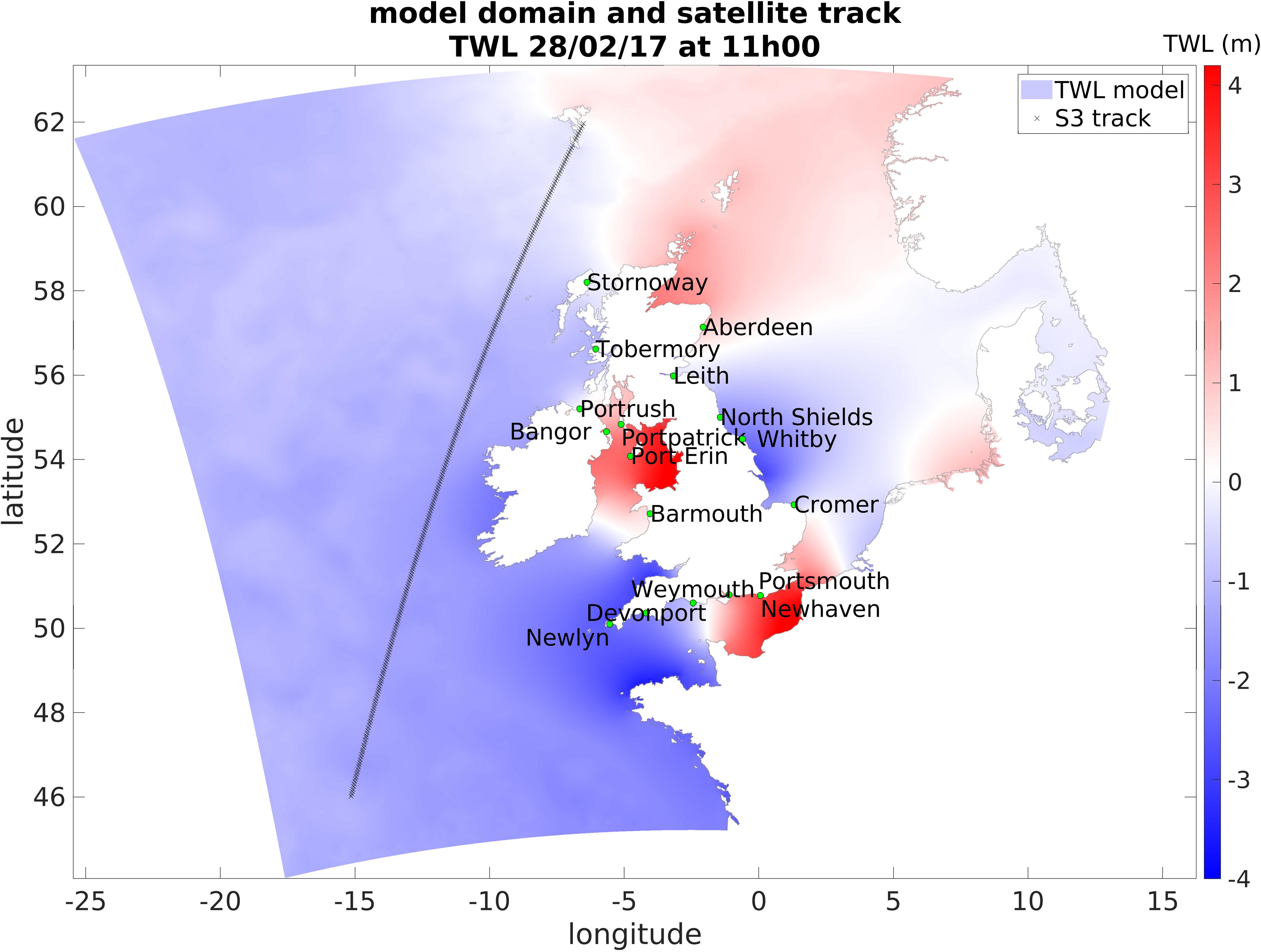
Figure 1. Snapshot of Amm15 coupled model domain showing TWL at 1100h on 28 February 2017 during Storm Ewan. The respective Sentinel-3 satellite track over the domain in that hour is also shown. The locations of the tide gauges used for comparisons with the satellite data are marked on the plot with green dots.

Total water levels can be evaluated using coastal TGs (Woodworth et al., 2015) or satellite data (Calafat et al., 2017). Here, we consider “still” TWLs, which are the joint contribution of astronomical tides and surges, excluding the influence of waves and changes in the mean sea surface (MSS). Despite the high accuracy of TG observations, they come with some limitations: tide gauges provide a good temporal resolution but have limited spatial coverage. In contrast, satellite altimeters provide (near-) global coverage but poor temporal sampling (generally, every 10 days or longer depending on the satellite) (Soumekh, 1999; Musa et al., 2015) and with data quality issues near the coast (Cipollini et al., 2017). The application of numerical models to estimate TWLs allows some of the issues associated with the observation records to be addressed by providing information with uniform and high spatial and temporal coverage. The models also have their limitations because of physical processes and interactions that are not resolved by the model resolution and are poorly parameterized or missing in the model. Also, due to computational limitations, model simulations often need to be run on reduced spatial domains or on a lower than desired resolution. Overall, TWL is often estimated by a combination of observations and models, and many studies rely on both methods (e.g., Vousdoukas et al., 2016; Melet et al., 2018) to obtain an accurate TWL estimate.

Recent advances in altimetry techniques now allow for satellites to provide observations closer to the coast than before (Benveniste et al., 2019; Vignudelli et al., 2019), making them more suitable to investigate near-coastal sea-level change (Beckley et al., 2010; Cazenave et al., 2018). It was shown that satellite altimetry provides valid uncorrupted measurements of sea surface height (SSH) over the open ocean, but that obtaining accurate values in the last 10 km from land is still a challenge and calls for specialized coastal processing (Vignudelli et al., 2019). Many of these challenges have now been overcome with the new generation of Delay-Doppler or Synthetic Aperture Radar (SAR) altimeter instruments such as those flying on-board CryoSat-2 or Sentinel-3, which can provide uncorrupted data as close as 1 km from land under favorable conditions (e.g., track orientation to the coast).

Following these ideas, sea level records from TGs, satellite observations, and predictions from a state-of-the-art numerical model are applied to the estimation of the TWL within 100 km from the United Kingdom coast. Data from seventeen TGs located around the United Kingdom and two recent SAR altimetry missions (CryoSat-2, Sentinel-3A) are used alongside high-resolution coupled model simulations from the Atlantic Margin Model (Amm15). The aim is to examine the consistency between satellite and model data and analyze the differences, when and where they agree or disagree, advantages and disadvantages, to understand what our capability is to represent the total water level in coastal and shelf seas when combining the potential of both satellite observations and numerical modeling. The structure of the paper is as follows: The data and methodology are described in section “Data and Methods.” Results are presented in section “Results” and then discussed in section “Discussion.” A summary and conclusions are in section “Conclusion.”

Data and Methods

Tide Gauge Data

Tide gauges data were obtained from the British Oceanographic Data Centre (BODC) for the period between 01 June 2016 and 30 September 2017. Data from seventeen TGs from United Kingdom and Ireland are used. Locations are shown in Figure 1. The records provide measurements averaged every 15 min and are used to compare with the model and satellite data in regions close to the coast. Data can be downloaded at https://www.bodc.ac.uk/data/hosted_data_systems/sea_level/uk_tide_gauge_network/.

Satellite Data

A new set of high resolution satellite altimetry data in SAR mode is obtained from the Copernicus Sentinel-3A (S3) satellite (ACRI-ST IPF Team, 2017). The S3 sea surface height anomaly (SSHA) includes contributions to water levels due to the tides and surges. Data is available at 1 Hz posting rate (approximately every 7 km along the satellite track) with the orbit repeating exactly every 27 days. The S3 data was obtained from the EUMETSAT distribution accessible at https://coda.eumetsat.int and https://codarep.eumetsat.int.

The period considered in the paper is from 01 June 2016 to 30 December 2017. The S3 product provides the SSHA as a variable, from which we obtain the TWL by adding back the corrections for ocean tide, the contribution from atmospheric pressure as expressed by the inverse barometer effect, and the barotropic contribution from wind to high-frequency sea level variability (modeled using the Mog2D model). We note that the provided SSHA has had the standard altimetric corrections applied, including the tropospheric (wet and dry) and ionospheric path delays, and the sea state bias. The surface classification flag (surf_class_01), the ocean backscatter coefficient flag (swh_ocean_qual_01_ku), and the altimeter range flag (range_ocean_qual_01_ku) available within the S3 products were then used to remove erroneous observations from the dataset.

The second set of altimeter data was taken from the SAR Interferometric Radar Altimeter (SIRAL) instrument on-board the ESA CryoSat-2 mission (C2). In this case, the 1 Hz data covered the period from 01 June 2016 to 30 September 2017. Contrary to S3, C2 has more closely spaced ground tracks but a much longer repeat cycle of 369 days. Here we use data from the CryoSat-2 Level 2 Geophysical Ocean Products (GOP), which are distributed by ESA and are available for download via ftp at ftp://science-pds.cryosat.esa.int. We refer the reader to the CryoSat Product Handbook¹ for a detailed description of the GOP data.

For C2 GOP, SSHA data is not provided and the TWL is computed as follows. First, we subtract the corrected range from the altitude to obtain the SSH, and we then subtract the DTU10 (Andersen, 2010) and MSS from the SSH to obtain the total SSHA (here total means that no geophysical correction has been applied at this point). The corrected range is defined as the range corrected for tropospheric and ionospheric path delays, and for sea state bias. The TWL is then obtained by correcting the total SSHA for the solid earth, loading, and pole tides. Hence, both the ocean tide and the barotropic atmospheric contributions are retained. To remove anomalous records, we reject all records that have been flagged as bad by the quality control flags provided within the product files. The corrections held in the data products for S3 and C2 are not the same and therefore it is not possible to repeat the exact same calculations for both satellites.

It is important to recognize that some of the altimetric corrections applied to the S3 and C2 data come from different sources and so might be different. This could lead to differences between the two altimetry datasets that would not be reflective of differing performances of the altimeters. It is important to keep this possibility in mind when interpreting the results of our analyses.

Numerical Model Data

The numerical model used in this paper is the regional coupled high-resolution Atlantic Margin Model (Amm15; Lewis H. W. et al., 2019), a coupled model joining the WaveWatch III (WW3; Tolman, 2014) numerical wave model to the NEMO ocean circulation model (Nucleus for European Modeling of the Ocean, NEMO; Madec and Nemo Team, 2008). The prescribed atmospheric forcing comes from ECMWF (Janssen and Bidlot, 2018). The configuration used is the ocean-wave coupled setting with no data assimilation (referred to as CPL_FR in Lewis H. W. et al., 2019); the ocean model is coupled hourly to exchange information with the wave model. The domain is set on the North Western European shelf, with a spatial resolution of 1.5 km at the coast and 3 km across deep ocean regions. TWL data from the model are given with respect to the model equipotential reference level and include both tide and surge processes. Details of the meteorological forcing, boundaries and initial ocean conditions are described in Tonani et al. (2019).

Quality Control and Collocation Processing

Total water level output from Amm15 (ocean-wave coupled) was compared against S3 from June 2016 to December 2017. The model output was compared to both S3 data and C2 data for the period from June 2016 to September 2017. Sixteen months of data are covered by both satellites, which allows cross-comparison of the model data with both satellites over the same period.

The satellites are first compared to local in-situ observations from TGs allowing the inclusion of a third independent dataset in coastal areas. Observations taken at in-situ TGs may be influenced by physical processes that the numerical model does not account for, they may also differ from the satellites observation due to the distance between the satellite track and the local TGs. Therefore, when deciding which TGs are appropriate to compare with the satellite and only using sites where the model performs best, the Amm15 model was compared to all BODC TGs recording between the 01 June 2016 and 30 September 2017. Only sites with more than 0.95 correlation and less than 0.30 m RMSE when compared to the model’s closest point in space (within 1.5 km) were considered in this work. Based on these criteria and on visual inspection of the records, 17 high-quality TGs located in United Kingdom and Ireland were selected. When comparing the satellite with TG data, only altimetry observations within 50 km from land and within 100 km from the TGs were used. To reduce the noise from altimetry records, the median value of all data recorded along the satellite track meeting the separation criteria and within the same minute was considered. The TGs values were interpolated in time to match the satellite overpasses. As some noise was still present in the records, the points where the difference in TWL between the satellite and the TG was more than 5 m were considered invalid and excluded from the comparison.

Data from both satellites within the model domain (Figure 1) was selected and the model point closest to an observation was identified for all satellite data points. Observations and model data were considered co-located if they were within 0.02° (∼2 km) of each other in space, and within 30 min of each other in time. Quality control was applied to S3 and C2 data to remove occasionally large outliers, mainly close to land. Different quality control approaches had to be used for S3 and C2. For the S3 satellite, the flags provided within the product were used. For C2, as too much noise remained in the records despite quality flags, the altimeter points that differed by more than 10 m from the model were considered invalid. These were all the coastal points where land contamination can impact satellite records, or where the model considered a specific cell as land whilst the satellite recorded valid data (or vice versa). Subsequently, all data outside 2 standard deviations (SD) from the mean difference between the model and satellite were removed. This criterion was chosen because it made it possible to discard obvious outliers from the records, yet it did not affect the part of the dataset that is of interest to this study. The area close to the model boundary was also removed to avoid accounting for model computational errors or linked to the changing model resolution (1.5 km to 3 km grid) in this region. The final area considered for the satellite-model comparison spanned [20°W;10°E] in longitude and [46°N, 62°N] in latitude (Figure 1).

Case Study Experiments

The satellites observations are compared to in-situ TGs selected using the numerical model to assess data in coastal areas (Table 1). The average RMSE is evaluated within 100 km from the TGs. As these are close to the coast, proximity to the TG also indicates proximity to land. However, altimeter data can be close or over land without being close to the TG, therefore both the distances between the satellite and TG as well as between satellite and land are considered in the analysis.

TABLE 1

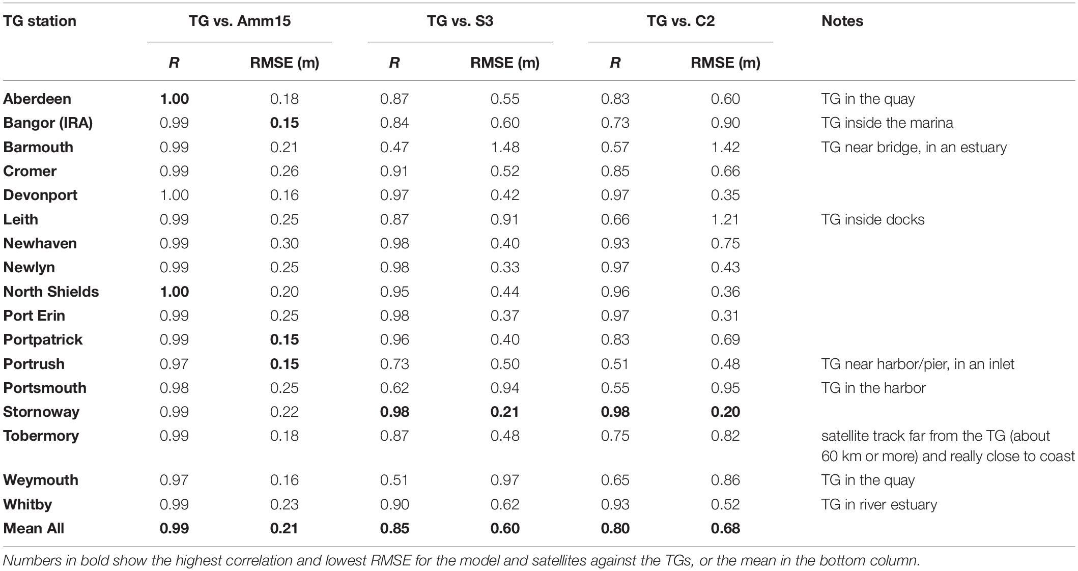
Table 1. Comparison of model and satellites to tide gauges.

To assess the capability of the satellites and the model in reproducing the TWL during storms, the periods with and without storm events between June 2016 and September 2017 were considered separately. Several storm events named by the Met Office occurred during the period considered (Angus, 20th November 2016; Barbara, 23rd–24th December 2016; Conor, 25th–26th December 2016; Doris, 23rd February 2017; Ewan, 25th–26th February 2017; Met Office, 2017) and three storm Surges were recorded on Surge Watch (16th October 2016; 19th November 2016; 13th January 2017; Haigh et al., 2017). The correlation, SD of the bias and RMSE error between altimetry and model data was estimated for the periods with and without storm events. One specific short-term event is kept as an example to show how the TWL is reproduced during the period between 25th February and 3rd March 2017, when storm Ewan occurred (Kendon et al., 2018).

An extended model-data comparison using S3 and Amm15 was analyzed over 19 months from June 2016 to December 2017, focused on understanding whether there is a bias between the model and observations. Since the S3 orbit repeats every 27 days, the same tracks will be covered about once a month, which means that multiple satellite observations are available over the same area even though they are 1 month apart. Co-located points were found during the period from June 2016 to December 2017. The bias between model and satellite was calculated along track during this period using repeated observations over the same locations.

Statistics evaluating the differences between the satellites and model data were also calculated for each month from June 2016 to September 2017 for both satellites. The monthly RMSE between satellite and model were evaluated for each point along track, as well as R and SD for each month (Table 2). February 2017 is used as an example in the discussion.

TABLE 2

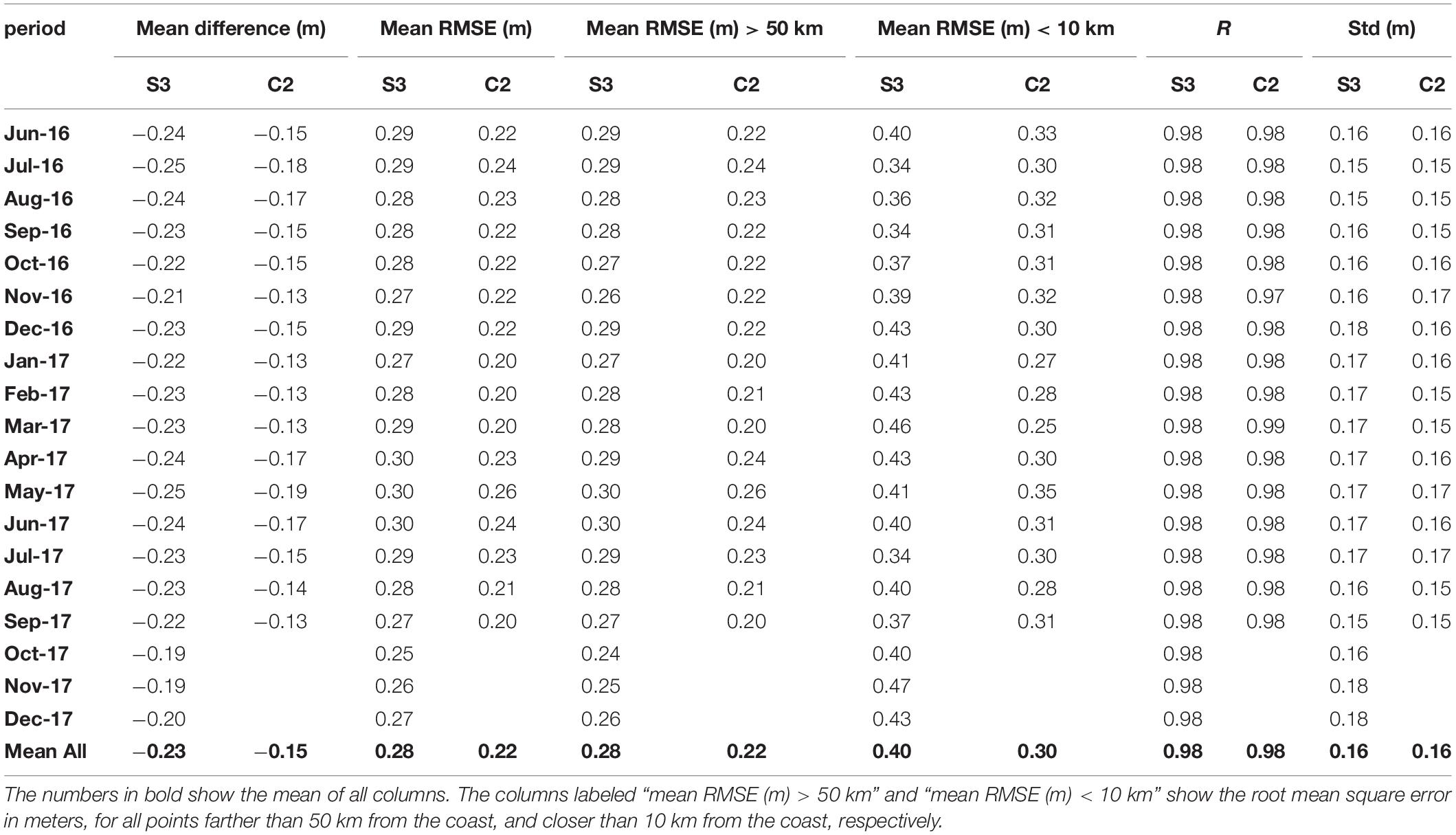
Table 2. Amm15 model compared to Sentinel-3A from June 2016 to December 2017, and CryoSat-2 from June 2016 to September 2017.

This set of data was also used to understand how well the sea surface can be observed when getting close to the coast in typical conditions, and how the offset compared to the model changes as a distance from the coast. For each month during the period studied with both satellites the RMSE was evaluated for all points within 10 km from land and further than 50 km from the coast (Table 2). To focus on the error variation as a function of distance from land, for the first 100 km from the coast the mean RMSE was evaluated for each km bin, and then plotted to observe changes in the error magnitude.

Results

A snapshot of the model hourly output with the respective satellite track covered during that time is shown in Figure 1, representing the TWL between 1100 and 1200 on the 28 February 2017 during storm Ewan. The TWL can vary by up to 8 m within a few degrees in space. Within this 1 h period the satellite crosses most of the latitudes in the domain, sampling data every second over different areas.

The two satellites used in this study have different orbits illustrated by a short-term case study in Figure 2. Physically adjacent tracks can indicate very different water levels. This is because each track will be recorded at a different time. Unlike C2, the S3 satellite repeats its orbit over the same coordinates every 27 days, therefore considering a short-term case study allows only a single use of any given track. As an example, the period between 25 February 2017 and 03 March 2017, during which storm Ewan hit the United Kingdom, was considered.

FIGURE 2

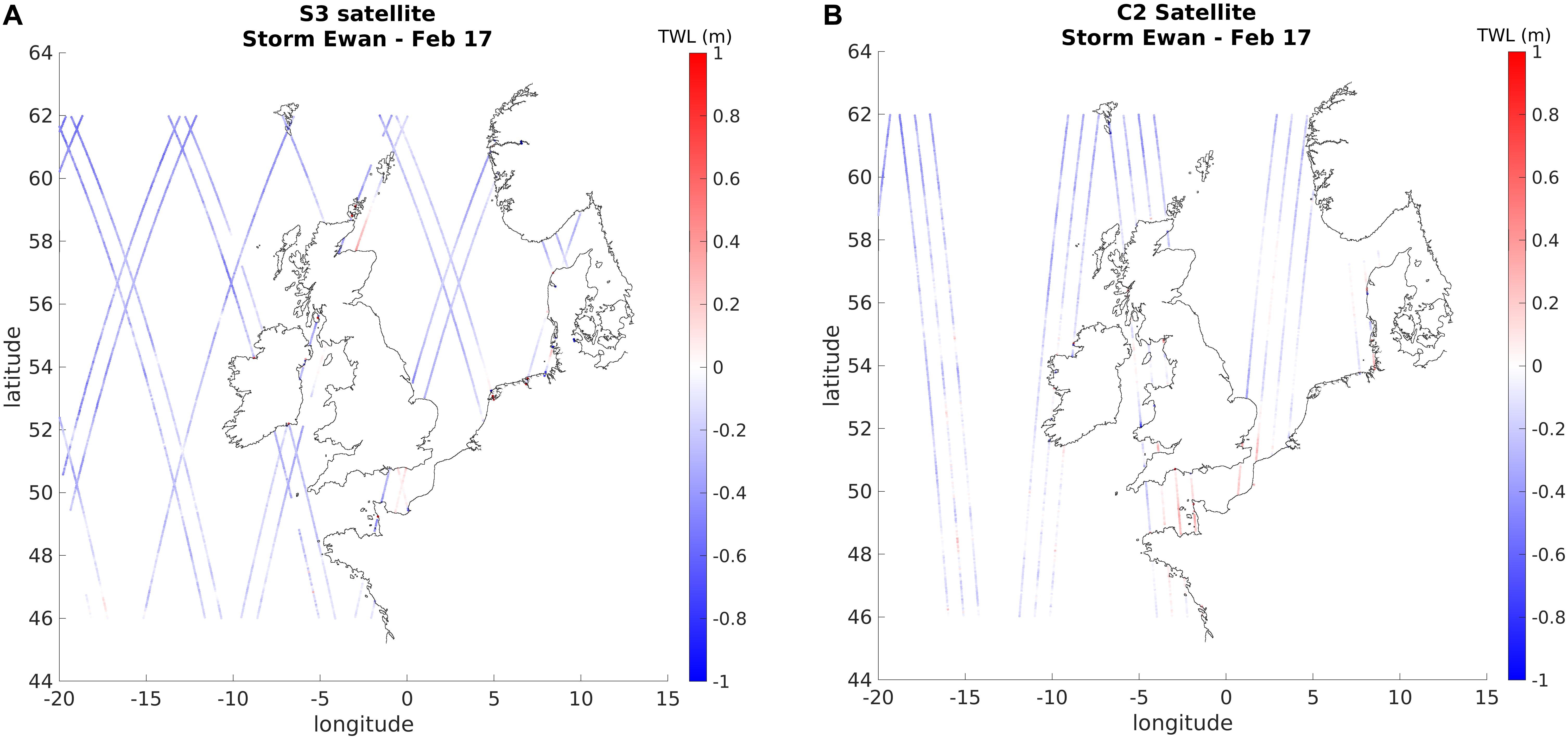
Figure 2. (A) TWL difference between Amm15 and S3 for the 7-day period between 25 February 2017 and 03 March 2017 during Storm Ewan. (B) TWL difference between Amm15 and C2 for the 7-day period between 25 February 2017 and 03 March 2017 during Storm Ewan.

The satellites are first compared to TGs in areas where the model can resolve the TWL (Table 1 and Figures 3, 4). The comparison between S3 and the TG shows a correlation ranging from 0.47 in Barmouth (RMSE = 1.48 m) to 0.98 in Stornoway (RMSE = 0.21 m), while for C2 the correlation ranges from 0.51 in Portrush (RMSE = 0.48 m) to 0.98 in Stornoway (RMSE = 0.20 m). The lowest correlation values are found at sites where the TG is enclosed within a harbor, port or land feature that is likely to degrade the performance of the altimeter. The average correlation with the TGs is 0.85 for S3, and 0.80 for C2.

FIGURE 3

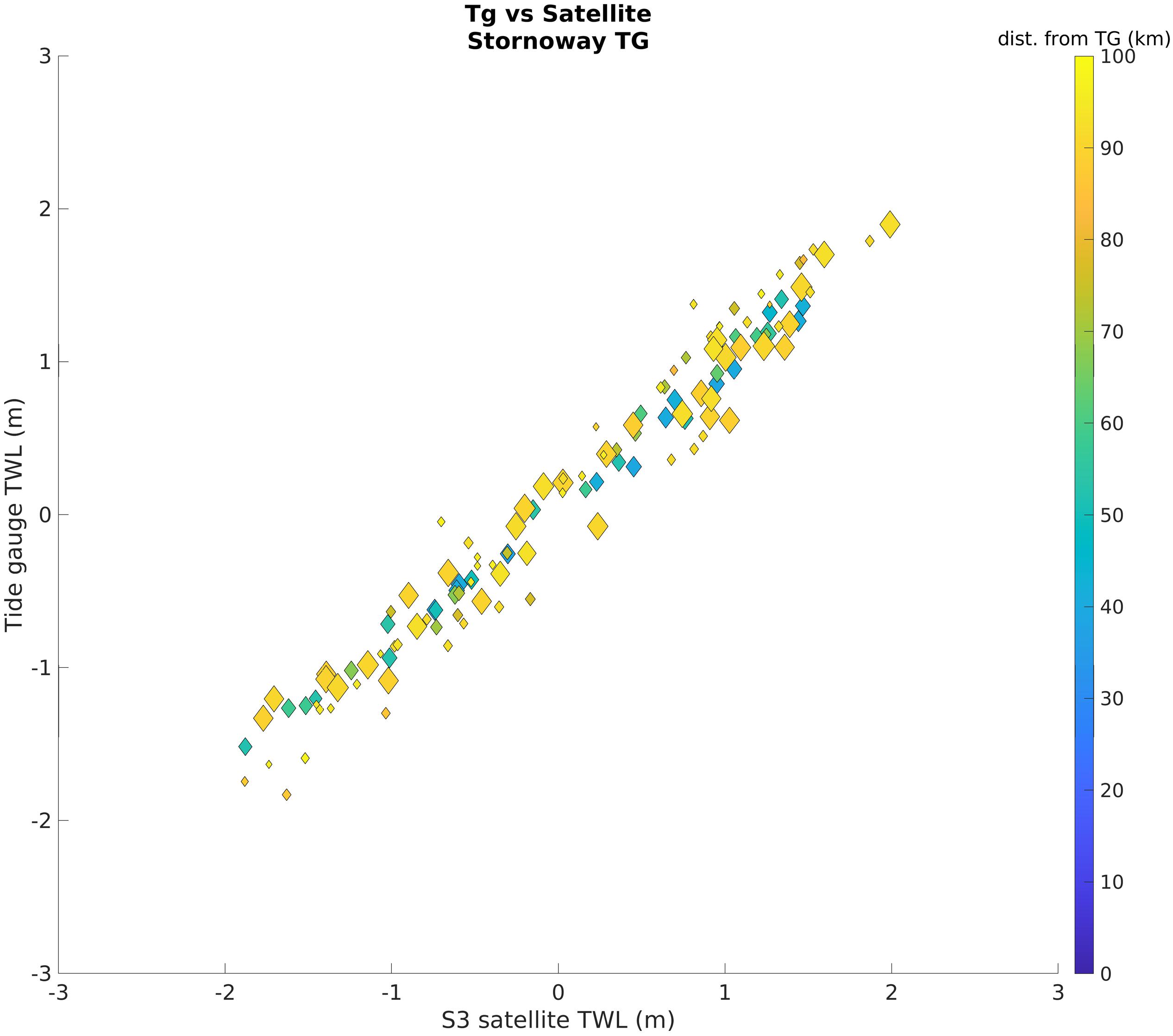
Figure 3. Comparison of S3 with TG at Stornoway, which had the lowest error of all stations considered. The color shows the distance of the Satellite from the TG (blue is at the TG location; yellow is up to 100 km away from the TG). The marker size indicates the distance of the satellite from the coast (The smallest markers are within 1 km of the coast, the widest markers are up to 50 km from the coast). Note that the distance of the satellite from the TG has a smaller impact than the distance to the coast over the results.

FIGURE 4

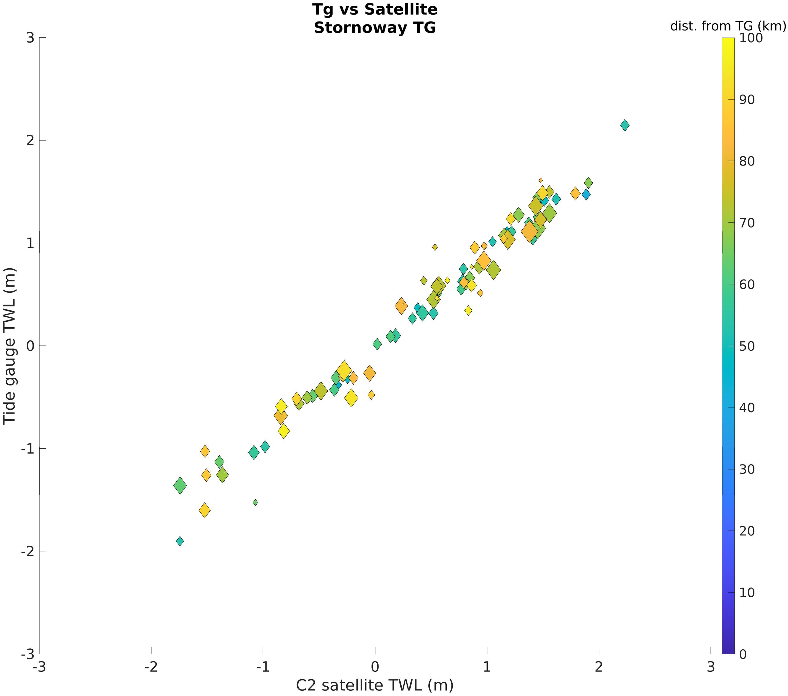
Figure 4. Comparison of C2 with TG at Stornoway, which had the lowest error of all stations considered. The color shows the distance of the Satellite from the TG (blue is at the TG location; yellow is up to 100 km away from the TG). The marker size indicates the distance of the satellite from the coast (The smallest markers are within 1 km of the coast, the widest markers are up to 50 km from the coast). Note that the distance of the satellite from the TG has a smaller impact than the distance to the coast over the results.

When considering the satellite data recorded in periods without storms as opposed to periods with storms (Figures 5, 6), R, SD, and RMSE remains similar. Between S3 and Amm15 R = 0.98 and RMSE = 0.28 m in both cases. The RMSE of points within 10 km from the coast shows an increase in RMSE of 0.01 m during periods with storms. The SD varies between 0.16 m in quiet periods and 0.17 m in stormy ones. Conversely, the RMSE between C2 and the model decreases during storm periods (reducing during storms by 0.02 m overall and 0.04 m close to the coast) and the SD of data goes from 0.16 m in quiet periods to 0.15 m during storm days. It must be noted that the number of sampling points during storm periods is about thirty times lower than that of non-stormy periods.

FIGURE 5

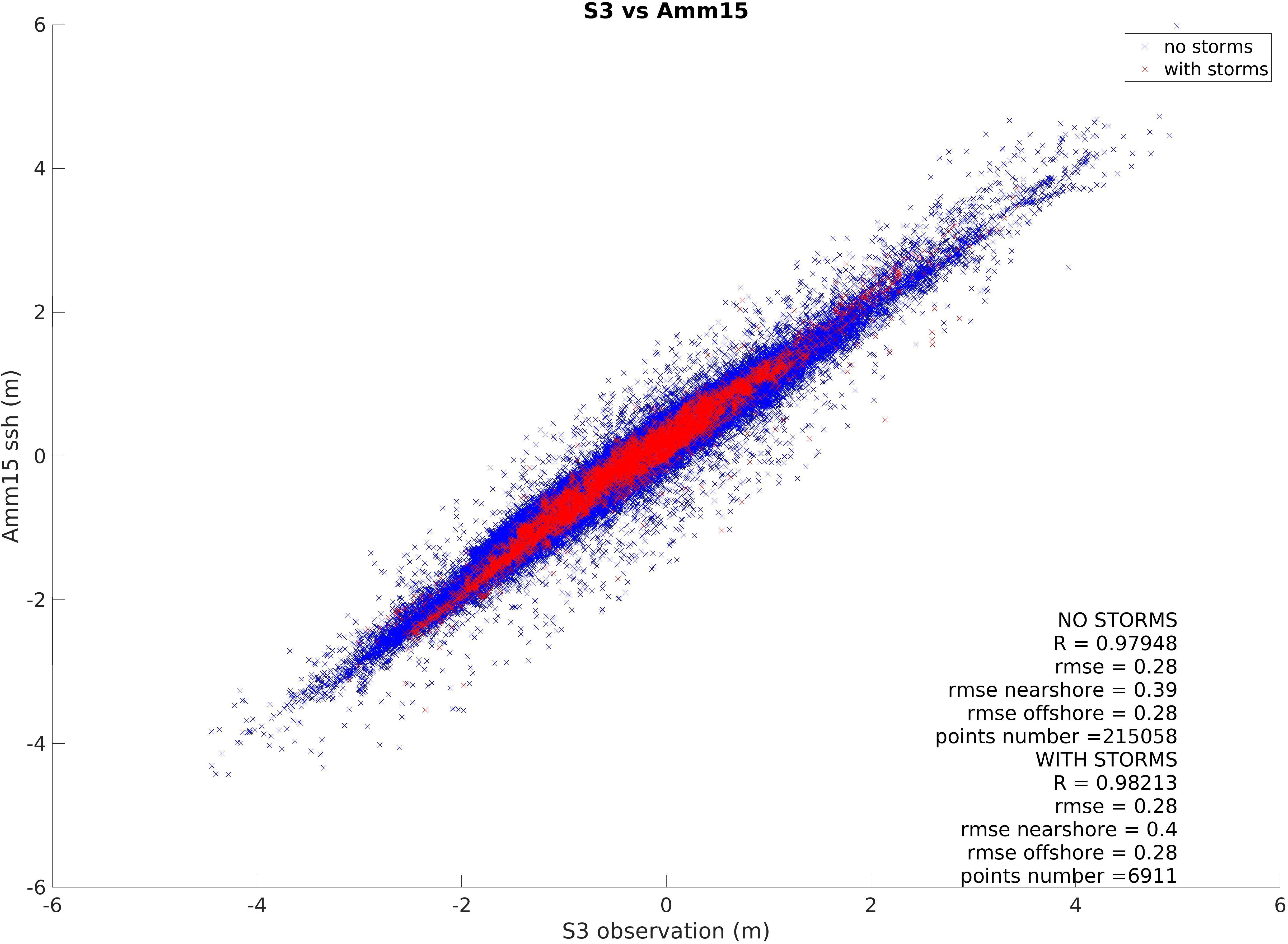
Figure 5. Correlation between S3 and Amm15 during period with and without storms. The plot also shows the statistics calculated from values closer than 10 km from the coast (near shore) or further than 50 km from the coast (offshore).

FIGURE 6

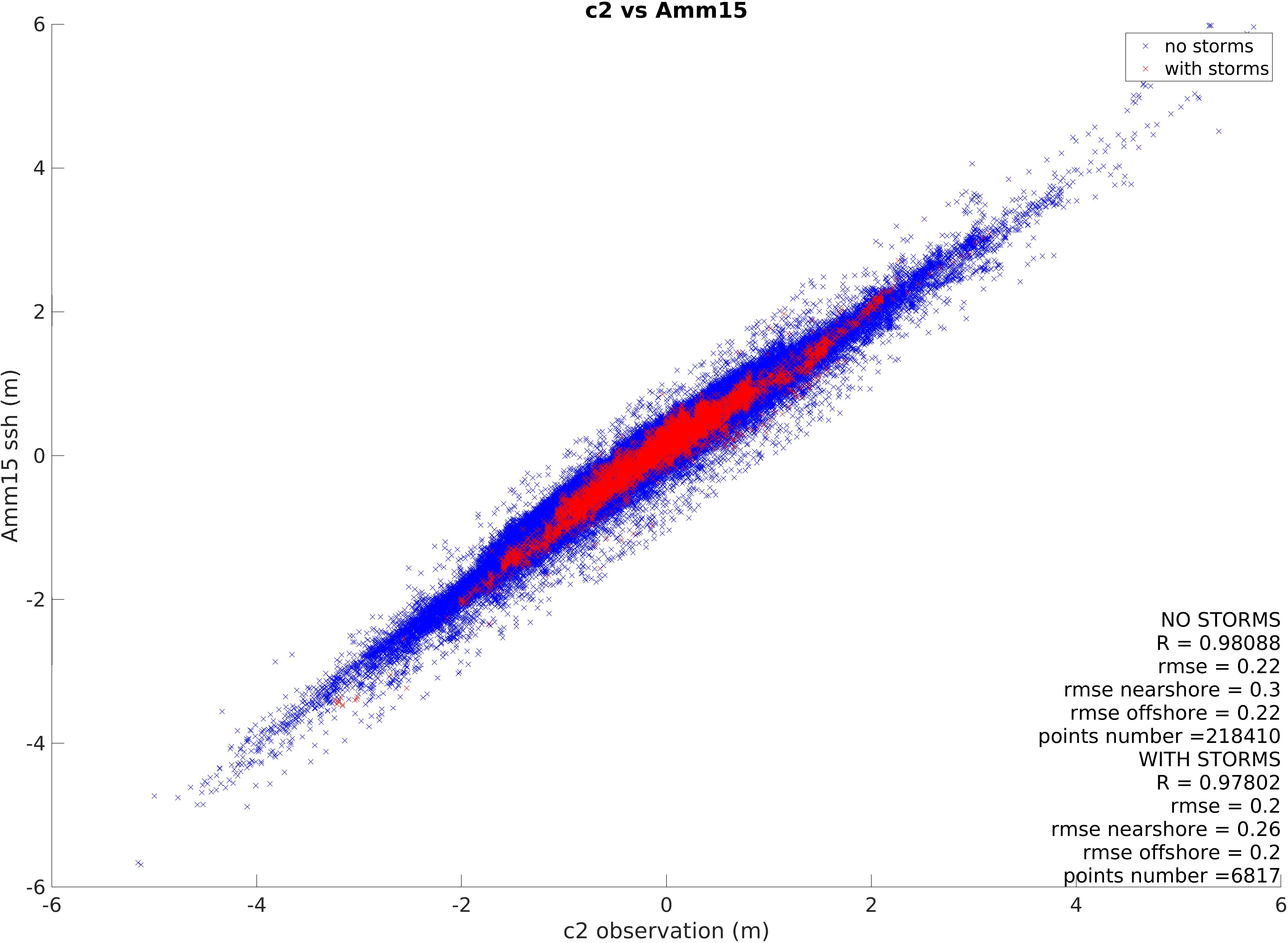
Figure 6. Correlation between C2 and Amm15 during period with and without storms. The plot also shows the statistics calculated from values closer than 10 km from the coast (near shore) or further than 50 km from the coast (offshore).

In the long time-interval comparison of S3 (Figure 7), the difference between the model and satellite over the repeating track of 19 months is of −0.23 m, with the largest values close to the coast. The average bias for each point over the entire period (Figure 7) shows that regions with high tidal range have better agreement between satellite and model. In the Straight of Dover, the North-East Irish Sea, and the German Bight the differences are lower than over the rest of the domain. However, when looking at each repeat period individually the tracks with the largest differences are in these same areas of high tidal range (English Channel, Irish sea, Bristol channel or German Bight).

FIGURE 7

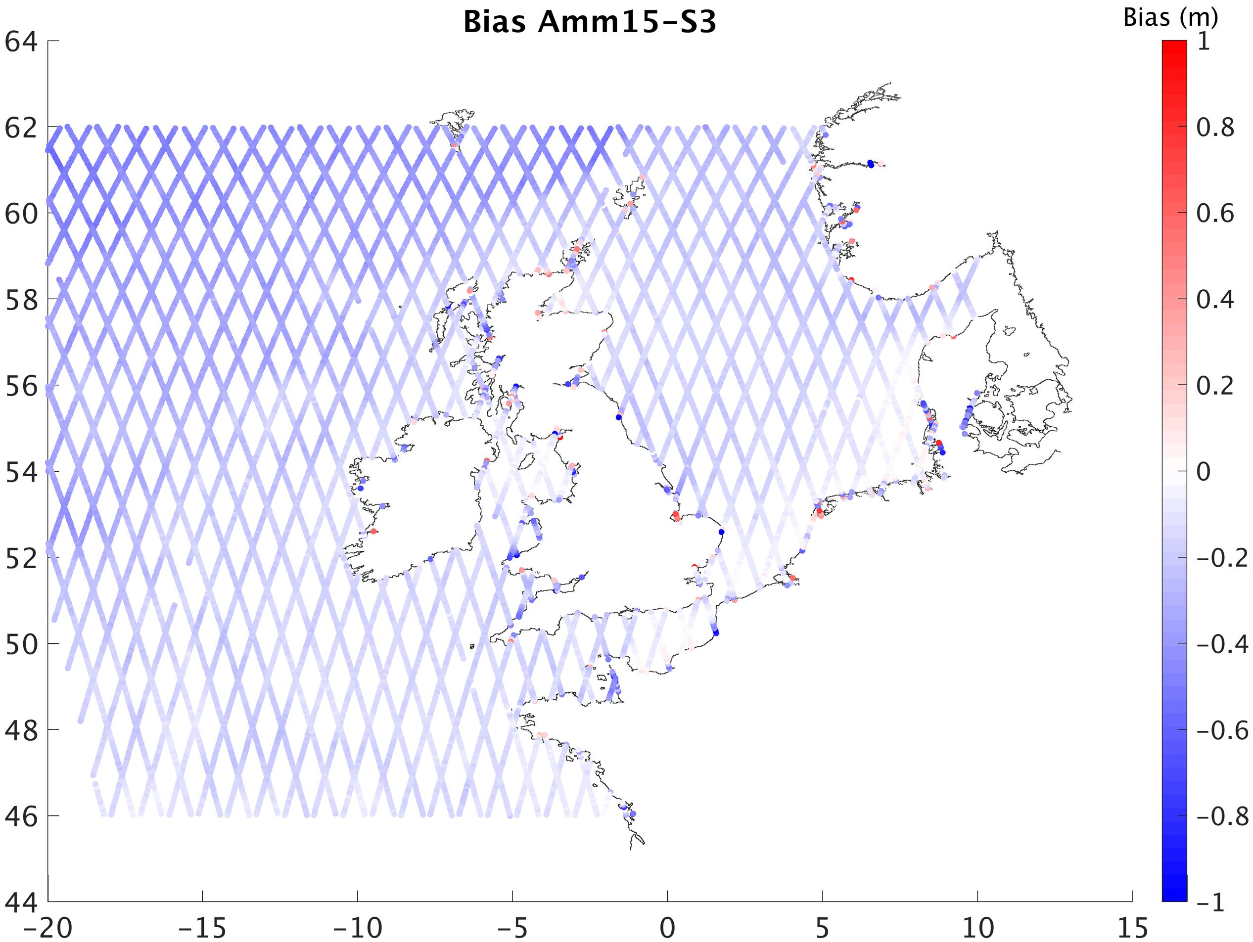
Figure 7. Mean bias between model and satellite observations along repeating tracks between June 2016 and December 2017.

Considering the TWL data from both satellites and the model, there is a good fit between results (Table 2), but the model is underestimating the S3 observations with a mean difference of −0.23 m, a RMSE of 0.28 m, and a SD of 0.16 m. The SD ranges between 0.15 m in July 2016, August 2016, and September 2016 and 0.18 m in December 2016, November 2017, and December 2017. Amm15 is also underestimating the C2 observations with a mean difference of −0.15 m, a RMSE of 0.22 m and a SD of 0.16 m. This difference is more pronounced when the satellite data is close to land.

The RMSE for S3 data farther than 50 km from the coast (Figure 8) varies between 0.24 and 0.30 m, with the highest RMSE in April 2016, May, and June 2017. When assessing data within 10 km of land, the error increases showing a much clearer seasonal variation (Figure 8). In this case the RMSE varies between 0.34 m in July 2016, September 2016, and July 2017, and 0.47 m November 2017 for S3, with the error tending to reduce during summer months. For the comparison of the C2 satellite (Figure 9), the error of data within 10 km from land varies between 0.25 m in March 2017 and 0.35 m in May 2017, while that of data farther than 50 km from land varies between 0.20 m in January, March, and September 2017, and 0.26 m in May 2017.

FIGURE 8

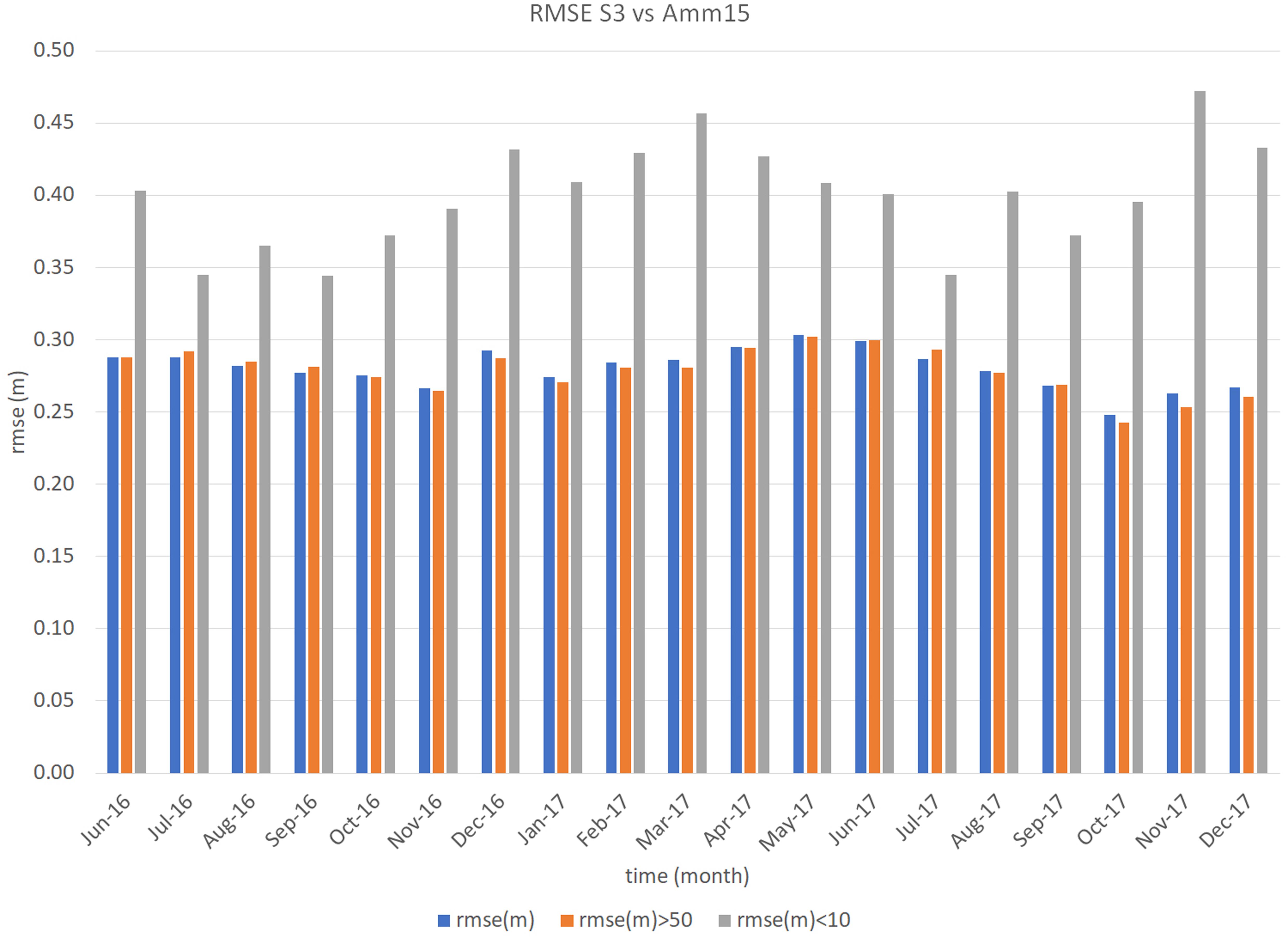
Figure 8. Statistics for the Amm15-S3 comparison. Mean monthly results from June 2016 to December 2017 (for Amm15-S3).

FIGURE 9

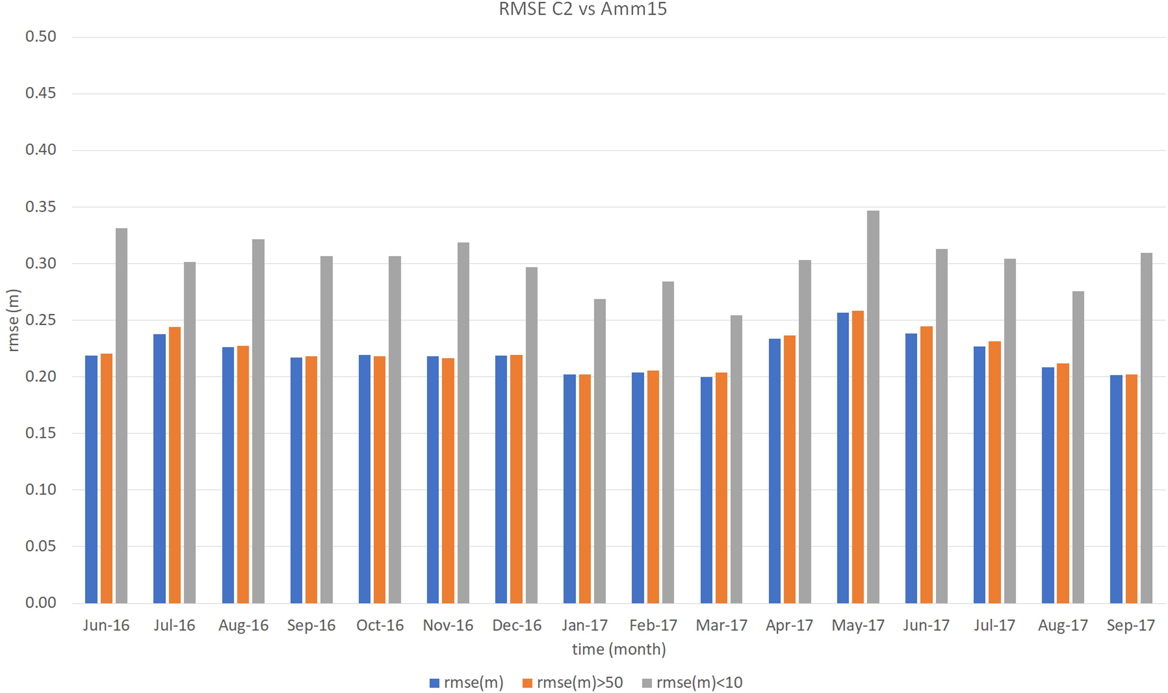
Figure 9. Statistics for the Amm15-C2 comparison. Mean monthly results from June 2016 to September 2017 (for Amm15-C2).

All points with lower agreement are coastal points (Figures 10A,B). However, it is important to note that a lot of coastal points with high correlation are present. Overall, the correlation between model and satellite was about 0.98 each month, although it must be noted that the tide dominates the signal, which is not necessarily representative of how well the satellite is reproducing the surge. Focusing on the last 100 km from the coast (Figures 10A,B) shows that the error tends to reduce away from land. Data within the last 3–4 km are noisier. Over 19 months of S3 data, the correlation evaluated per km bins only drops from 0.98 in the center of the basin to 0.97 at 4 km from land and reaches 0.95 at 3 km from land, while for the 16 months of C2 the correlation remains 0.98 up to (and including) 4 km from land, lowering to 0.96 at 3 km.

FIGURE 10

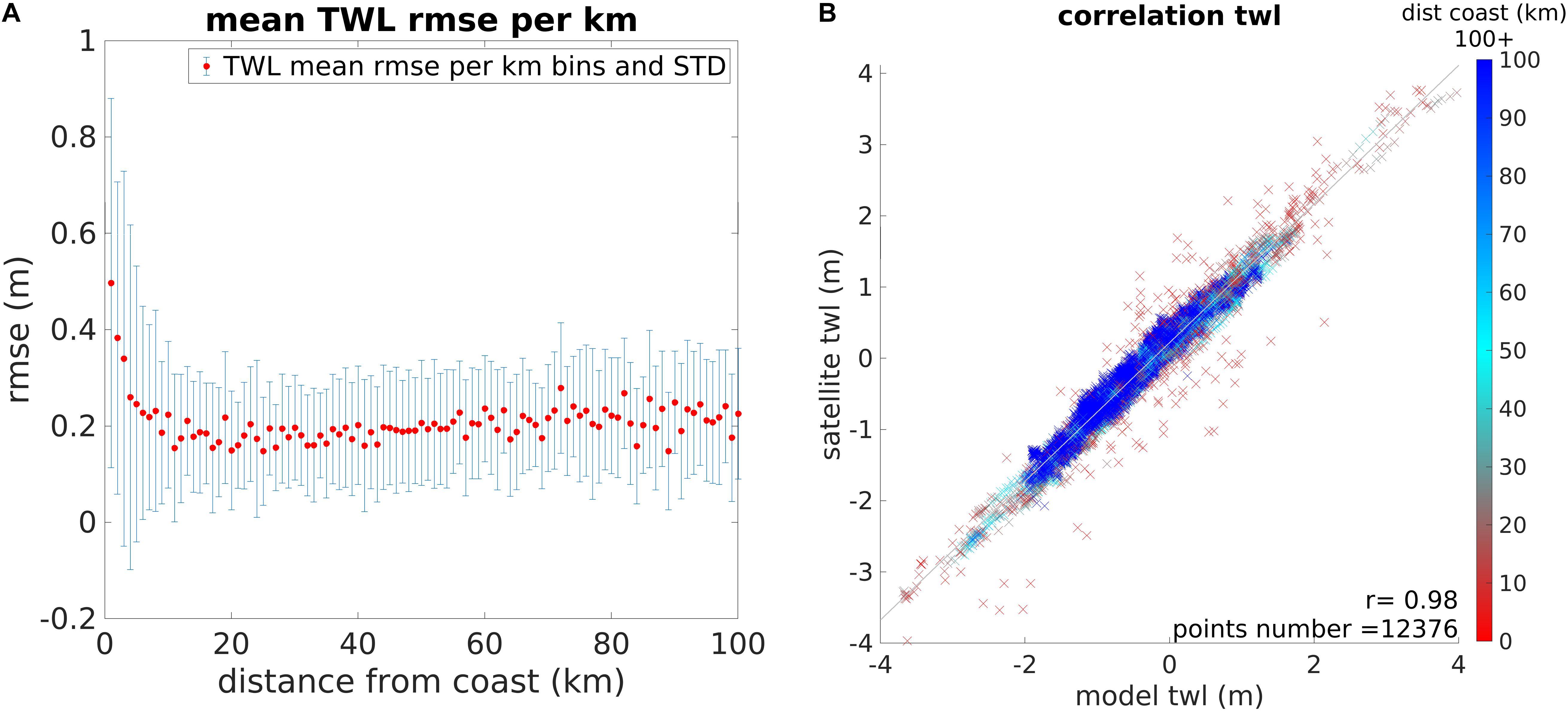
Figure 10. (A) RMSE of the TWL difference between S3 and Amm15 as function of the distance from the coast. This example is from February 2017. (B) Correlation between satellite and model data with color indicating distance to the coast from (blue) all data further than 100 km from the coast to (red) data at the coast. The RMSE in the right plot was averaged per kilometer bins.

Discussion

Comparison to TGs

To analyze data in the coastal regions, which are the most challenging for altimeters (Vignudelli et al., 2019), the satellite data was compared to observations from seventeen TGs. As these are close to the coast, proximity between the satellite tracks and the TG does not always translate into a good agreement because of land contamination and inaccurate corrections affecting the altimeter performance (Figures 3, 4). Results show that the satellite can correlate well with TGs, with higher error when the site is located within a harbor or close to features that may interact with the satellite footprint. In these cases, the use of the model can be helpful to complement the observations. Considering all stations, the correlation between the two kinds of observation is on average 0.85 (S3) and 0.80 (C2), with a maximum value of 0.98 in Stornoway for both satellites (RMSE of 0.21 m for S3 and 0.20 m for C2). Results show that the difference between TG and satellite is lower when the satellite is close enough to the gauge to observe the same area, but not close enough for the land to affect results. The lowest RMSE in our comparison is 0.20 m, which is comparable to the difference between satellite and model, however, in this case this difference cannot be due to an offset in time between the two measurements, but will more likely be due to the distance between the satellite observation and the TG.

Long Term Comparison Between the S3 Satellite and Model

Comparing S3 and Amm15, the most interesting result is the consistent −0.23 m difference between satellite and model over 19 months. This nearly constant bias is understood to be induced by the differences in the reference levels used by the model and the satellite. The latter relates its mean sea level to the WGS84 ellipsoid, whereas the Amm15 TWL output are referenced to the model’s equipotential reference level. Other studies with accurate calibration of the geoid reference level and satellite correction specific to the study area showed biases of only a few centimeters when comparing both S3 and C2 data to tidal gauges (Bonnefond et al., 2019). These calibrations required in-situ field work that could not be repeated in this study.

Moreover, the satellite provides extremely high frequency data at 1 Hz giving practically instantaneous measurements, whilst the model outputs hourly data, therefore the closest point in time between model and satellite can be up to half an hour away. In this time, the tide in this area can change of about 0.2 m, which is comparable to the S3-Amm15 differences (Figures 7, 8). Presumably when only considering points closer in time, the difference between model and satellite due to the variation in tidal stage should reduce. There was an attempt to demonstrate this by only comparing model and satellite points closer than half an hour in time, but the number of sampling points that can be considered varies so much that it was not possible to draw conclusions from this experiment.

Another point underlining the impact of the tidal stage is that the highest equinoctial spring tide in 2017 occurred on the 28 April², when some of the highest errors appear in the results. Moreover, even though areas with high tidal range are better represented by model and satellite considering the overall mean over 19 months, these regions showed a high variability in the results when looking at individual repeat period. The areas with high tidal range showed tracks with some of the major errors in an individual month, but these were different tracks each month therefore this does not appear in the mean bias plot. This again suggests that the timing between the satellite and model might affect results. A half an hour lag in time will appear more obvious in these regions of high tidal range, even though over all these areas are better represented.

Impact of Storms Events

Altimetry measurements are increasingly used to complement observations from TGs in order to study storm surges (Antony et al., 2014) or to improve surge forecast by assimilating observations to models (De Biasio et al., 2017). Their application to the monitoring and forecasting of surges is developing and increasingly used, one of the most recent initiatives being the European Space Agency’s eSurge project³. Satellite observations have the advantage of covering the open ocean areas which cannot be observed by tide gauges, but the poor temporal sampling means that not all storm events might be captured. For the altimeter to capture the surge there is a reliance on coincidence between the satellite track and the storm time. While this provides extremely valuable information, altimetry measurements must often be used combined with other data source to accurately study surges and storms. In this study, the highest monthly RMSE (Figures 8, 9) often occurs in periods hit by either storms, surges, or extreme wave events. However, looking in more details and considering the dates affected by storms or surges separately from those without them, the RMSE and correlation between both satellites and the model does not vary much (Figures 5, 6). Note that the error scales with the magnitude of the storm is absolute, not normalized. The correlation remains of 0.98 in either cases, while the RMSE only varies of up to 0.04 m in regions within 10 km from land with the C2 data. The S3 comparison to the model has a slightly lower RMSE (0.01 m difference within 10 km from land) in periods without storms, while for C2 the opposite happens. In this case the RMSE decreases by 0.02 m offshore and 0.04 m near land during periods with storms. The SD for S3 data is 0.17 m with storms and 0.16 m without them, while for C2 the SD of data is 0.15 m with storm and 0.16 m without them. It must be considered that the number of sampling points during storm periods (6911 for S3, 6817 for C2) is more than thirty times lower than that of periods without storms (215058 for S3, 218410 for C2), which will affect these differences. It must also be noted that some minor storms or extreme wave events that have not been considered here could have happened during that period. Looking at storms individually, some events showed a higher difference between model and satellite than throughout other periods, without there being any obvious difference to the number of passes over land. Overall, the results show that the altimetry data can capture TWL during storms as well as in quiet periods.

Evaluating How the Error Changes as a Function of the Distance From the Coast

The coastal region has always been the most complex area for both models and satellites when evaluating sea level changes. However, as the value of both altimetry observation and accurate simulations in this region are widely recognized, increasing efforts are made to improve the quality and accessibility of such data. For altimetry, improving observations within the last 10 km from land has been the focus of several coastal altimetry studies in recent years (Cipollini et al., 2009), with projects such as Coastal Altimetry (COASTALT)⁴ funded by the European Space Agency (ESA). In this study, when analyzing data considering distance from the coast, it appears that the correlation between model and satellite tends to reduce when getting closer to land. In most cases, considering both the S3-Amm15 and the C2-Amm15 comparison, the only regions where the RMSE (averaged per kilometer bin) exceeded 0.3 m was within 3–4 km from land (Figure 10B). The correlation of data (Figure 10A) plotted considering the distance of each point along track from the nearest coast shows that all the major discrepancies between satellite and model data are at the coast. However, there is also a significant number of coastal points where model and satellite are in good agreement. The RMSE of data within 10 km from the coast varies between 0.34 and 0.47 m over S3’s 19 months comparison, and between 0.25 and 0.35 m for C2’s 16 months. Moreover, other studies pointed out how noise due to land contamination can interfere with the accuracy of both S3 and C2 data in coastal areas (Vignudelli et al., 2019). These near shore regions can be better observed using high frequency data, such as 20 Hz frequency (Birgiel et al., 2018), which were not used in this study. Also, altimetry products based on coastal-dedicated re-trackers, such as the Adaptive Leading Edge Subwaveform (ALES) re-tracker (Passaro et al., 2014), provide higher quality data close to the coast and their use is recommended when the focus is on the coastal zone. Nevertheless, it is increasingly recognized that standard products from SAR altimeters such as S3, can provide coastal data of comparable quality to data processed with dedicated coastal re-trackers. Indeed, results from our study show that there is a good fit between satellite and model data up to 4 km from land, which is similar to the closest distance to coast that coastal re-trackers can achieve on average.

Remaining Uncertainties and Future Work

This analysis shows significant differences between the comparisons of S3-Amm15 and the C2-Amm15. The variability of data is extremely consistent in both cases, with higher disagreement close to the coast and in areas of high tidal range, however, it is striking that the mean bias appeared to be significantly lower in the C2-Amm15 comparison than in the S3-Amm15 case. Therefore, in the following part of the discussion we attempt to understand whether this is significant. The better agreement between C2 and the model could be due to the differences between the satellites, which have a unique reference frame offset and sea state bias. The RMSE was improved from an average of 0.28 m over the 19 months of S3 observations to 0.22 m for the 16 months of C2 observations. Improvements are visible especially over the open ocean, but also in coastal areas (Table 2 and Figures 10A,B). Within 10 km from land the RMSE values reduced to an average of 0.30 m when comparing the coupled model to the C2 satellite, as opposed to an average of 0.40 m in the S3-Amm15 comparison. Another issue that needs to be resolved is that of the reference level difference between model and satellite. It is important to quantify what that difference is to better compare the data. Other studies mention issues related to the geoid slope affecting results (Fenoglio-Marc et al., 2015) and the use of high-resolution geoid models was shown to improve S3 validation over coastal areas (Birgiel et al., 2018). To assess this in future work the difference between the model and satellite reference level will need to be resolved. As this study highlights, the absolute reference level is important in relatively short (19 months) time scales, and not relevant only when studying longer time-scale changes in mean sea level.

Moreover, there are more complex coupled models available which include atmospheric models as well as oceans and waves, such as the UKC3 in development at the Met Office (Lewis H. et al., 2019). It was not possible to use this tool in the present study, however, the incorporation of the atmosphere could have an interesting impact over results and should be used in future studies. It would allow tracking of the storms through the atmosphere data and check the location of surges with respect to the satellite assessing in greater details the accuracy of observation during storm events.

This analysis also shows that some storm events led to an increase in the RMSE compared to the average over the long time-interval, however, considering all storms that were registered during the period of study, there is no significant difference between the error for data recorded over periods with or without storms. More work should be done over individual events to understand why that is.

Conclusion

Results showed that in all cases there is a good fit between satellite and model with a 0.98 mean correlation, which is also reflected in the comparison of the satellites to TGs. Between June 2016 and December 2017, the monthly mean difference between the S3 satellite and the Amm15 model is −0.23 m, and −0.15 m for C2 between June 2016 and September 2017. The comparison is affected by the time lag between satellite and model data, which means there can be a phase difference in the tidal stages compared. This is especially visible over areas with high tidal range, which show the greater variability in the data error. These areas, however, are better represented looking at the overall bias of the repeated S3 track points between June 2016 and December 2017. Moreover, there appears to be a link between the presence of some storms and the absolute error although, overall, the RMSE and correlation between the satellites and model is similar whether storms are included or not. More work should be done to understand why specific storm events lead to higher discrepancies.

The coast is the most difficult area to resolve for both satellite and model, but in this comparison, observations and simulations are consistent close to land and discrepancies increase only 3–4 km from land (R equal 0.97 at 4 km from the coast and 0.95 at 3 km from it for S3, and R equal 0.98 up to 4 km from land, lowering to 0.96 at 3 km for C2). Within 10 km from the coast the RMSE varies between 0.34 and 0.47 m over 19 months comparison (S3), and between 0.25 and 0.35 m for the 16 months comparison (C2). Other studies show how the coastal region is better observed by high frequency 20 Hz data, as opposed to the 1 Hz considered in this study (Passaro et al., 2014; Birgiel et al., 2018), which should be used if working close to land. Both satellites and models can provide useful information complementing tide gauges observation in these regions, however, more work needs to be done to further improve the accuracy of data at the coast. The comparison to TG data in this case showed that the correlation with both satellites could be as high as 0.98, and the RMSE as low as 0.21 m for S3 and 0.20 m for C2, however, the location of TGs with respect to the track greatly influence the results. To exploit the relative advantages of both observations and simulation, previous studies have assimilated satellite altimetry data to surge models, improving the forecast of extreme events (De Biasio et al., 2017). While altimetry data alone can be used to study storms and extreme events (Antony et al., 2014), we believe that in future work the best approach would be to consider observations and simulation as complementary to each other, especially when applied to the study of coastal regions where uncertainties increase in both methods.

Uncertainties remain about the differences between the S3-Amm15 comparison and the C2-Amm15 comparison. More work needs to be done to reduce the systematic bias between the two satellite, and between satellite and the model. A better understanding of the bias will not only improve the inter-comparison but will have important implications for the use of these observations for studying extreme coastal water levels and changing mean sea-level.

In conclusion, from the data analyzed it appears that the discrepancies between satellite and model can increase during large storm or surges, but overall the RMSE of data recorded during storm periods is similar to that of periods without them and the altimeter can observe both equally well. The tidal range was shown to have an effect over the accuracy of the results because there can be a time lag between the simulations and the observations compared. The winter and spring seasons also had higher error for S3, probably in relation to a higher number of storms in these periods. The discrepancies between data also increase near the coast, however, results are consistent up to 4 km from land, which demonstrate the improvement in satellite altimetry’s near shore records, as well as the importance of numerical modeling as a tool to resolve the coastal regions along with other observational records. In future work it will be important to better understand the sources of bias between satellites and models with respect to their differences in reference levels. It will also be interesting to investigate the impact of storm surges and tidal stage over the accuracy of both instruments, which could lead to important developments. Overall, from the data used in this study, the satellite altimetry data and the model appeared to be extremely consistent with each other, even in most of the coastal areas. Through a synthesis of these independent datasets, we have great confidence in the representation of TWL.

Data Availability Statement

The datasets presented in this article are not readily available because these data are of the order of the tens of terabytes. Requests to access the datasets should be directed to the Met Office. S3 satellite data EUMETSAT distribution is available at: https://coda.eumetsat.int and https:// codarep.eumetsat.int. C2 satellite data ESA distribution is available at: ftp: //science-pds.cryosat.esa.int. Further inquiries can be directed to the corresponding author.

Author Contributions

JR, FC, LB, and JAMG designed the research. JR lead the study, performed the research and the data analysis, and produced the figures. FC fundamental help with data analysis/interpretation and provided CryoSat data. CB provided Sentinel-3A data and a supervisor during this work. LB help with data analysis/interpretation and fundamental help in developing the manuscript. CG help with data interpretation and display of information and help with acquisition of information about the previous work done by the satellite altimetry team. JAMG help with data interpretation, work management and fundamental help in developing the manuscript. IH helped drafting and revising the work. HL provided the numerical model data and helped understanding all aspects related to the numerical model. AM supervised the project related to this study and fundamental help in data analysis and interpretation. FC, CB, CG, and AM help learning and understanding satellite altimetry processes and difficulties related to this kind of observation. All authors contributed to the article and approved the submitted version.

Funding

This work used Monsoon2, a collaborative High-Performance Computing facility funded by the Met Office and the Natural Environment Research Council. This research has been carried out under national capability funding as part of a directed effort on UK Environmental Prediction, in collaboration between Centre for Ecology & Hydrology (CEH), the Met Office, National Oceanography Centre (NOC) and Plymouth Marine Laboratory (PML). Part of this work has been carried out as part of the Copernicus Marine Environment Monitoring Service (CMEMS) Ocean-Wave-Atmosphere Interactions in Regional Seas (OWAIRS) project. CMEMS is implemented by Mercator Ocean in the framework of a delegation agreement with the European Union. JR, FC, CG, CB, and AM have been partially supported by the EU contract 730030 call H2020-EO-2016 ‘CEASELESS’.

Conflict of Interest

The authors declare that the research was conducted in the absence of any commercial or financial relationships that could be construed as a potential conflict of interest.

Footnotes

1. ^ https://earth.esa.int/documents
2. ^ https://www.ntslf.org/tides/hilo
3. ^ http://www.storm-surge.info/esurge
4. ^ http://www.coastalt.eu/

References

ACRI-ST IPF Team (2017). MPC for the COPERNICUS SENTINEL-3 MISSION Product Data Format Specification - OLCI Level 1 Products. ESA and EUMETSAT. Available online at: https://sentinel.esa.int/documents/247904/1872756/Sentinel-3-OLCI-Product-Data-Format-Specification-OLCI-Level-1

Google Scholar

Andersen, O. B. (2010). The DTU10 gravity field and Mean sea surface. Paper Presented at the Second International Symposium of the Gravity Field of the Earth (IGFS2), Fairbanks, Alaska, United States.

Google Scholar

Antony, C., Testut, L., and Unnikrishnan, A. S. (2014). Observing storm surges in the Bay of Bengal from satellite altimetry. Estuar. Coast. Shelf Sci. 151, 131–140. doi: 10.1016/j.ecss.2014.09.012

CrossRef Full Text | Google Scholar

Beckley, B. D., Zelensky, N. P., Holmes, S. A., Lemoine, F. G., Ray, R. D., Mitchum, G. T., et al. (2010). Assessment of the Jason-2 extension to the Topex/Poseidon, Jason-1 sea-surface height time series for global mean sea level monitoring. Mar. Geod. 33, 447–471. doi: 10.1080/01490419.2010.491029

CrossRef Full Text | Google Scholar

Benveniste, J., Cazenave, A., Vignudelli, S., Fenoglio-Marc, L., Shah, R., Almar, R., et al. (2019). Requirements for a coastal hazards observing system. Front. Mar. Sci. 6:348. doi: 10.3389/fmars.2019.00348

CrossRef Full Text | Google Scholar

Birgiel, E., Ellmann, A., and Delpeche-Ellmann, N. (2018). “Examining the performance of the sentinel-3 coastal altimetry in the baltic sea using a regional high-resolution geoid model,” in Proceedings of the 2018 Baltic Geodetic Congress (BGC Geomatics), Olsztyn.

Google Scholar

Bonnefond, P., Exertier, P., Laurain, O., Guinle, T., and Féménias, P. (2019). Corsica: a 20-Yr multi-mission absolute altimeter calibration site. Adv. Sp. Res. (in press). doi: 10.1016/j.asr.2019.09.049

CrossRef Full Text | Google Scholar

Calafat, F. M., Cipollini, P., Bouffard, J., Snaith, H., and Féménias, P. (2017). Evaluation of new CryoSat-2 products over the ocean. Remote Sens. Environ. 191, 131–144. doi: 10.1016/j.rse.2017.01.009

CrossRef Full Text | Google Scholar

Cazenave, A., Palanisamy, H., and Ablain, M. (2018). Contemporary sea level changes from satellite altimetry: what have we learned? what are the new challenges? Adv. Sp. Res. 62, 1639–1653. doi: 10.1016/j.asr.2018.07.017

CrossRef Full Text | Google Scholar

Chartteron, J., Clarke, C., Daly, E., Dawks, S., Elding, C., Fenn, T., et al. (2016). The Costs and Impacts of the Winter 2013 to 2014 Floods. Available online at: https://www.gov.uk/government/publications/the-costs-and-impacts-of-the-winter-2013-to-2014-floods (accessed September 10, 2019).

Google Scholar

Cipollini, P., Benveniste, J., Bouffard, J., and Al, E. (2009). “The role of altimetry in coastal observing systems,” in Proceedings of the OceanObs’09: Sustained Ocean Observations and Information for Society, Southampton.

Google Scholar

Cipollini, P., Calafat, F. M., Jevrejeva, S., Melet, A., and Prandi, P. (2017). Monitoring sea level in the coastal zone with satellite altimetry and tide gauges. Surv. Geophys. 38, 33–57. doi: 10.1007/s10712-016-9392-0

PubMed Abstract | CrossRef Full Text | Google Scholar

De Biasio, F., Bajo, M., Vignudelli, S., Umgiesser, G., and Zecchetto, S. (2017). Improvements of storm surge forecasting in the Gulf of Venice exploiting the potential of satellite data: the ESA DUE eSurge-Venice project. Eur. J. Remote Sens. 50, 428–441. doi: 10.1080/22797254.2017.1350558

CrossRef Full Text | Google Scholar

Fenoglio-Marc, L., Dinardo, S., Scharroo, R., Roland, A., Dutour Sikiric, M., Lucas, B., et al. (2015). The german bight: a validation of cryoSat-2 altimeter data in SAR mode. Adv. Space Res. 55, 2641–2656. doi: 10.1016/j.asr.2015.02.014

CrossRef Full Text | Google Scholar

Haigh, I. D., Ozsoy, O., Wadey, M. P., Nicholls, R. J., Gallop, S. L., Wahl, T., et al. (2017). An improved database of coastal flooding in the United Kingdom from 1915 to 2016. Sci. Data 4, 1–10. doi: 10.1038/sdata.2017.100

PubMed Abstract | CrossRef Full Text | Google Scholar

Home Office (2017). National Risk Register of Civil Emergencies, 2017 Edn, Available online at: www.official-documents.gov.uk (accessed January 23, 2020).

Google Scholar

Janssen, P. A. E. M., and Bidlot, J. R. (2018). Progress in operational wave forecasting. Procedia IUTAM 26, 14–29. doi: 10.1016/j.piutam.2018.03.003

CrossRef Full Text | Google Scholar

Kendon, M., McCarthy, M., Jevrejeva, S., Matthews, A., and Legg, T. (2018). State of the UK climate 2017. Int. J. Climatol. 38, 1–35. doi: 10.1002/joc.5798

CrossRef Full Text | Google Scholar

Lewis, H., Manuel Castillo Sanchez, J., Arnold, A., Fallmann, J., Saulter, A., Graham, J., et al. (2019). The UKC3 regional coupled environmental prediction system. Geosci. Model. Dev. 12, 2357–2400. doi: 10.5194/gmd-12-2357-2019

CrossRef Full Text | Google Scholar

Lewis, H. W., Manuel Castillo Sanchez, J., Siddorn, J., King, R. R., Tonani, M., Saulter, A., et al. (2019). Can wave coupling improve operational regional ocean forecasts for the north-west European Shelf? Ocean Sci. 15, 669–690. doi: 10.5194/os-15-669-2019

CrossRef Full Text | Google Scholar

Madec, G. NEMO Team (2016). NEMO Reference Manual 3_6_STABLE: NEMO Ocean Engine, Note du Pôle de Modélisation, Institut Pierre-Simon Laplace (IPSL), France, No. 27 ISSN, No. 1288–1619.

Google Scholar

Melet, A., Meyssignac, B., Almar, R., and Le Cozannet, G. (2018). Under-estimated wave contribution to coastal sea-level rise. Nat. Clim. Chang. 8, 234–239. doi: 10.1038/s41558-018-0088-y

CrossRef Full Text | Google Scholar

Met Office (2017). UK Storm Season 2016/17. Available online at: https://www. metoffice.gov.uk/weather/warnings-and-advice/uk-storm-centre/uk-storm-sea son-2016-17 (accessed July 18, 2020).

Google Scholar

Musa, Z. N., Popescu, I., and Mynett, A. (2015). A review of applications of satellite SAR, optical, altimetry and DEM data for surface water modelling, mapping and parameter estimation. Hydrol. Earth Syst. Sci. 19, 3755–3769. doi: 10.5194/hess-19-3755-2015

CrossRef Full Text | Google Scholar

Passaro, M., Cipollini, P., Vignudelli, S., Quartly, G. D., and Snaith, H. M. (2014). ALES: a multi-mission adaptive subwaveform retracker for coastal and open ocean altimetry. Remote Sens. Environ. 145, 173–189. doi: 10.1016/j.rse.2014.02.008

CrossRef Full Text | Google Scholar

Soumekh, M. (1999). Synthetic Aperture Radar Signal Processing with MATLAB Algorithms. New York, NY: Wiley.

Google Scholar

Tolman, H. L. (2014). User Manual and System Documentation of WAVEWATCH III^® Version 4.18. NOAA/NWS/NCEP/MMAB Technical Note 316, 282 + Appendices.

Google Scholar

Tonani, M., Sykes, P., King, R. R., McConnell, N., Pequignet, A.-C., Dea, E., et al. (2019). The impact of a new high-resolution ocean model on the Met Office North-West European Shelf forecasting system. Ocean Sci. Discuss. 15, 1133–1158. doi: 10.5194/os-2019-4

CrossRef Full Text | Google Scholar

Vignudelli, S., Birol, F., Benveniste, J., Fu, L. L., Picot, N., Raynal, M., et al. (2019). Satellite altimetry measurements of sea level in the coastal zone. Surv. Geophys. 40, 1319–1349. doi: 10.1007/s10712-019-09569-1

CrossRef Full Text | Google Scholar

Vousdoukas, M. I., Voukouvalas, E., Mentaschi, L., Dottori, F., Giardino, A., Bouziotas, D., et al. (2016). Developments in large-scale coastal flood hazard mapping. Nat. Hazards Earth Syst. Sci. 16, 1841–1853. doi: 10.5194/nhess-16-1841-2016

CrossRef Full Text | Google Scholar

Woodworth, P. L., Pugh, D. T., and Plater, A. J. (2015). “Sea-level measurements from tide gauges,” in Handbook of Sea-Level Research, eds I. S. Antony, J. L. Benjamin, and P. Horton (Hoboken, NJ: Wiley), 555–574. doi: 10.1002/9781118452547.ch35

CrossRef Full Text | Google Scholar