Spatial Structure of Low Salinity Submesoscale Features and Their Interactions With a Coastal Current

1. Introduction

Interactions between buoyancy-driven flows and coastal currents govern nearshore circulation along many coasts around the world. They are complex and influenced by several factors, such as freshwater discharge, winds, waves and tides that occur at various spatial and temporal scales. A buoyant layer insulates surface coastal water from deeper waters and amplifies the efficiency of wind forcing near the surface. At the same time, the lateral density gradient or pressure gradient formed between the buoyant plume and ambient seawater geostrophically alters the intensity of wind-driven currents. The fate and characteristics of buoyant plumes, as well as the currents, are therefore controlled by the interaction between the plume and wind-driven circulation.

It is evident that surface freshening and warming can hinder ventilation of the ocean by causing increased stratification (Somavilla et al., 2017). Pycnoclines induced from density increase between the surface waters and deeper waters create effective barriers to vertical mixing, limiting the vertical transport of energy and nutrients. This makes stratification relevant for climate processes and biogeochemical cycles. In much of the world's upper oceans, temperature variations dominate the spatial gradients and seasonal variations of density, whereas salinity plays a secondary role (Johnson et al., 2012; Ramachandran et al., 2018). However, in regions that are strongly influenced by rain and freshwater run-off, salinity variations can be the leading control on near-surface density gradients (Timmermans and Winsor, 2013; MacKinnon et al., 2016; Ramachandran et al., 2018). In these regions, the depth of the surface mixed layer is controlled by the vertical salinity gradient, while temperature can remain uniform or even change below the mixed layer (Jaeger and Mahadevan, 2018). Stratification caused by small scale features that have strong salinity gradients can influence vertical exchanges (Ramachandran et al., 2018). Strong stratification near the surface inhibits vertical fluxes of momentum, heat and tracers (Prasanna Kumar et al., 2003). The latter study showed that the resulting dynamical isolation of such strongly stratified surface layers from deeper nutrient-rich layers is a key factor explaining lower biological productivity in the Bay of Bengal on the eastern side of India compared to the Arabian Sea on the western side. The fate of freshwater injected into shelf seas can therefore have implications on ocean productivity.

The relative effect of temperature and salinity on density has been investigated for shelf seas (Timmermans and Winsor, 2013; Jaeger and Mahadevan, 2018) and for open oceans (Rudnick and Martin, 2002; Tippins and Tomczak, 2003; Johnson et al., 2012). Injection of substantial freshwater to shelf seas can change conditions suitable for a well-mixed unstable water column to statically stable, with strong stratification and less vertical mixing. In shelf seas, stronger drivers, such as wind and diurnal cooling are usually more prevalent mixing mechanisms compared to double diffusion. However, for the East China Sea, conductivity, temperature, and depth (CTD) measurements showed that double diffusion can be consistent with variations of temperature and salinity (Shi and Wei, 2007). In contrast, in the Chukchi Sea, temperature and salinity gradients measured from glider observations are non-compensating, with salinity changes dominating density gradients (Timmermans and Winsor, 2013).

Oceanic regions where river inputs, precipitation, ice-freezing and melting are major contributors to the near-surface density field, are likely to be “hot-spots” of submesoscale activity year-around (Luo et al., 2016). Submesoscale processes are therefore ubiquitous features in coastal waters. There are a number of processes that may inhibit the formation of instabilities in such coastal systems, such as frictional processes that dissipate motion (Hetland, 2017). Rivers play a key role in determining temperature-salinity (T-S) distributions and in governing cross-shelf transport processes (Barkan et al., 2017b). By comparing the Mississippi–Atchafalaya River system to other river systems, Hetland (2017) suggested that the evolution of a river plume is critical in determining if instabilities will occur or not. A river plume can become baroclinically unstable and advect offshore as a result of detachment of eddies that form in the plume's frontal zone (Chen et al., 2008).

Submesoscale processes influence upper ocean mixing and horizontal and vertical exchange of nutrients, which in turn impact ocean primary productivity. Various facets of the submesoscale regime have been studied previously including density stratification in the surface layer (Boccaletti et al., 2007), its role in the turbulent cascade of energy (Capet et al., 2008; Barkan et al., 2015; McWilliams, 2016), characterization of its coherent structures (Mahadevan and Tandon, 2006; Gula et al., 2014; McWilliams et al., 2015; Dauhajre et al., 2017), and potential ecosystem controls (Lévy et al., 2012, 2018; Mahadevan, 2016). Submesoscale processes, typically associated with spatial scales of O(1–10) km and temporal scales of O(days), are dynamically defined as having O(1) Rossby and Richardson numbers (Thomas and Ferrari, 2008). A range of submesoscale processes that may be active in the ocean mixed layer include baroclinic instability, symmetric instability, lateral shear instability, and frontogenesis (Thomas and Lee, 2005; Boccaletti et al., 2007; Capet et al., 2008; Fox-Kemper et al., 2008; Taylor and Ferrari, 2009; D'Asaro et al., 2011; Callies et al., 2015; Haney et al., 2015). In general, most submesoscale instabilities act to slump fronts, reduce mixed-layer depth, increase stratification and decrease vertical mixing (Thomas and Ferrari, 2008; Lévy et al., 2018).

In this study, we introduce the acronym “LSMF” for low-salinity submesoscale features which are buoyant features that propagate as submesoscale river plumes, or as plumes detached from their source under the condition of instability. We investigate the structure and stability of LSMFs originating from river discharges in a New Zealand shelf sea. The overarching aim is to understand the impact of strong salinity gradients on stratification and investigate the balance between wind driven stirring and baroclinic instability. The following questions will be addressed: What is the spatial structure of LSMFs? How do LSMFs impact local ambient stratification? What are the implications of LSMFs for mixing and subsequent primary production? What oceanographic conditions favor and constrain the advection of river-induced LSMFs? Section 2 will detail the field setting and section 3 will introduce the multi-platform approach applied in this study. In sections 4–6, we will describe the characteristics of spring LSMFs. In these sections we also distinguish and discuss three oceanographic regimes of LSMF offshore propagation. We close off section 6 by connecting our findings to other shelf sea systems.

2. Regional Setting: Central New Zealand Continental Shelf

Greater Cook Strait is the shelf sea region between the North and South Islands of New Zealand (Figure 1). The western side is wide and large, comprising of Golden Bay, Tasman Bay, and the South Taranaki Bight making up the Greater Cook Strait (170 km wide), leading through the Narrows on the eastern side (23 km wide) (Figure 1B). This New Zealand shelf sea is influenced by strong wind-driven and tidal currents (Walters et al., 2010). Consequently, the shelf is dominated by the response to a wind-forced flux (Cahill et al., 1991; Walters et al., 2010) through a large tidally-dominated, fast-flowing and weakly stratified strait (Stevens, 2014, 2018). Greater Cook Strait is also strongly influenced by freshwater influx from numerous small to medium rivers (Sutton and Hadfield, 1997; Cornelisen et al., 2011), throughflow due to surface elevation differences at the east and west open boundaries of the shelf and baroclinic currents due to density variations (Walters et al., 2010). This makes this New Zealand shelf sea an ideal set up for the investigation of the role of LSMFs on water column stratification, and barotropic and baroclinic interactions in shelf seas.

FIGURE 1

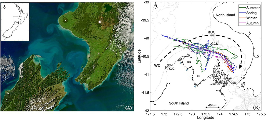
Figure 1. Map of (A) True color of Greater Cook Strait region cropped from image of New Zealand obtained by NASA's Aqua MODIS satellite for April 29, 2011; available on NASA's earth observatory. Map of New Zealand in top left corner, with Greater Cook Strait region highlighted as gray box. (B) Map of Greater Cook Strait showing general circulation of the region (WC: Westland Current and DUC: d'Urville Current), locations of GB: Golden Bay, TB: Tasman Bay, KUC: Kahurangi upwelling cell (striped region), FS: Farewell Spit, SI: Stephen Island and glider tracks (line color indicating the seasonal affiliation of each glider survey). Hotspots of low salinity submesoscale features (North of Farewell Spit and middle of Greater Cook Strait) are plotted in blue circles. Numbers 1–4 indicate locations of river mouths of Arorere River, Takaka River, Motueka River, and Waimea/Wairoa River, respectively.

The d'Urville Current dominates subtidal transport in Greater Cook Strait (Chiswell et al., 2015; Stevens et al., 2019). The current is primarily fed by the northward flowing Westland Current, and fluctuates in strength and frequency. This is due to weather-band variations in wind stress from south-westerly and westerly winds (Stanton, 1976; Shirtcliffe et al., 1990), and associated coastal-trapped waves (Cahill et al., 1991). With north-westerly winds, the Westland Current may reverse and flow southwards down the West Coast. Consequently, the strength and direction of the d'Urville Current in Greater Cook Strait may change with wind direction and subtidal flows (Harris, 1990).

Offshore Ekman transport generated by south-westerly winds also creates semi-permanent upwelling of deep saline water along the west coast (Heath and Gilmour, 1987; Harris, 1990; Shirtcliffe et al., 1990; Chiswell et al., 2016). Deep cold saline water is entrained into the Westland Current, forming the northward flowing Kahurangi plume and advected into Cook Strait by the d'Urville Current (Heath and Gilmour, 1987; Harris, 1990; Shirtcliffe et al., 1990). The dynamics of this Ekman-generated upwelling system has been documented by Chiswell et al. (2016) using satellite observations of surface temperature and chlorophyll-a. This shelf region also experiences near-surface water freshening from nearby rivers and precipitation (Harris, 1990). In Golden and Tasman Bays specifically, density is controlled by freshwater inputs and temperature gradients, caused by river discharges. Each bay has contributions from two main rivers: the Aorere and Takaka rivers into Golden Bay and the Motueka and Waimea/Wairoa rivers into Tasman Bay (Figure 1B). Recently Chiswell et al. (2019) confirmed that the mean velocity in Golden and Tasman Bays is weak and the circulation is dominated by wind and tidal flows. Mean near-surface velocity is generally out of each bay and is compensated for by inward circulation at depth.

3. Methods

3.1. Glider Surveys in Greater Cook Strait

Continuous, long-duration and high resolution hydrographic sampling from gliders have enabled the evaluation of variability in density structure of submesoscale features in a New Zealand shelf sea. Glider sampling allows for: (1) minimal disturbance of upper stratification and (2) horizontal and temporal spacing between profiles to be typically <1 km and 30 min depending on the profile depth.

Seven glider surveys were completed from 2015 to 2018 (Figure 1B); O'Callaghan and Elliott (2020). The average glider track spanned 40°75S,174°49E to 39°91S, 171°90E. In each survey, the glider transverses from east to west and back to its deployment location. For surveys 3, 4, 6, 9, and 11, the glider was deployed closer to the Cook Strait Narrows. As the glider would spend multiple days trying to overcome strong currents due to strong tidal fluctuations near the Narrows, deployments for surveys 12 and 15 were from Tasman Bay to maximize observations across the Greater Cook Strait shelf sea.

Bathymetry of Greater Cook Strait varies considerably across the shelf (40–130 m). Water depth shoals to <40 m in Golden and Tasman Bays and is > 150 m to the west beyond Farewell Spit. A single glider survey in Greater Cook Strait typically lasted 4 weeks, during which it sampled the water column in a sawtooth diving pattern between 0 and 200 m and covered over 500 km (horizontally). Vertical velocities of the vehicle were slower than 0.3 m s⁻¹ and 26,263 profiles were obtained from glider surveys between November 2015 and March 2018 (Table 1). On average, each dive cycle comprised six profiles which took 2 h and covered a horizontal distance of 2.5 km. This translated to a temporal resolution of ~ 20 min and a spatial resolution of ~ 0.4 km between each water column profile. The autonomous and continuous sampling at high spatial (horizontal and vertical) and temporal resolution allow small scale processes to be resolved (Rudnick, 2015).

TABLE 1

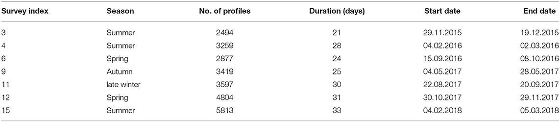
Table 1. Glider survey index, seasonal affiliation, number of profiles sampled, start and end dates of each glider survey completed in Greater Cook Strait.

This study used Teledyne Webb Research Slocum G2 gliders equipped with Seabird CTD sensor, Aanderaa Oxygen Optode and Wet Labs Environmental Characterization Optics (ECO) puck, that measured chlorophyll-a fluorescence, backscatter (at 470, 532, 660, and 700 nm) and chromophoric dissolved organic matter (CDOM). Temperature, conductivity, and pressure data were sampled at 0.5 Hz, and subsequently processed to remove spikes. The accuracy within calibration range of temperature and conductivity were ±0.002°C and ±0.0003 S m⁻¹, respectively. Glider data processing was completed using the SOCIB glider toolbox [https://github.com/socib/glider_toolbox; Troupin et al. (2015)]. Glider data processing includes salinity lag correction for the thermal lag error for the un-pumped CTD unit, which is standard on Slocum gliders (Pascual, 2010; Garau et al., 2011). Data were averaged in vertical bins of 1 m.

3.2. Identification of Observed Low-Salinity Submesoscale Features (LSMFs) From Glider Observations

A salinity threshold of ⩽ 34.75 psu in at least 10 consecutive profiles of each LSMF (at depth 10 m) was used to identify an observed LSMF. The chosen threshold was 0.45 psu below the 35.2 psu observed throughout most of Greater Cook Strait and was distinct from the ambient salinity. One exception was LSMF 4 from glider survey 6 which is the repeat sampling of LSMF 3 6 days later (Table 2). A threshold of ⩽ 34.85 psu was used to identify LSMF 4 as mixing of LSMF 3 occurred over this 6-days period.

TABLE 2

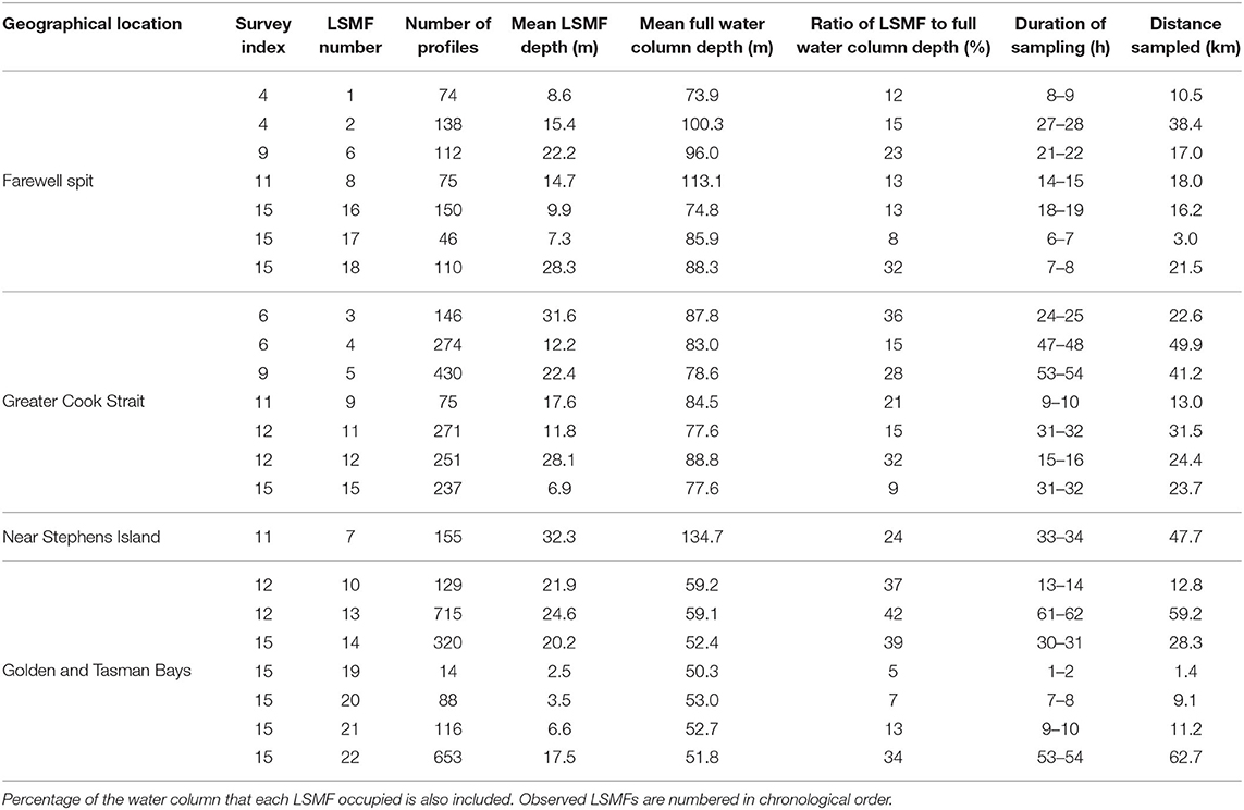
Table 2. Mean LSMF depth, survey index, LSMF number, full water column depth, duration of sampling, and distance sampled in each LSMF for each of the 22 observed LSMFs classified based on their geographical location.

Horizontal scales of the LSMFs was estimated by the distance covered by the glider between the first and last profiles with salinity ⩽ 34.75 psu. A similar approach was applied to evaluate the duration of sampling of LSMFs by combining times of the first and last profiles with salinity ⩽ 34.75 psu. The last depth layer with salinity ⩽ 34.75 psu would define the depth of the observed LSMF (vertical scale) for each profile. The mean LSMF depth of each feature was then calculated from all associated profiles. Ratio of LSMF depth to full water column depth was used to quantify what ratio of the water column the LSMFs occupy, since bathymetry within the study region varies considerably across the shelf. Full water column depth referred to the sum of maximum depth attained by the glider and its target altitude depth (of 8 m) for each profile. The distance covered by the glider vertically, horizontally and duration of sampling within each LSMF are summarized on Table 2.

3.3. Regional Modeling

Outputs from a Regional Ocean Modeling System (ROMS) for the period April 2, 2009 to September 2, 2012 (12-hourly averages) were used to contextualize regional scale interactions with LSMFs. ROMS is a free-surface hydrodynamic ocean model that uses the hydrostatic and Boussinesq approximations on an Arakawa C-grid, with a terrain-following vertical coordinate (https://www.myroms.org/). ROMS has widely been used in a range of coastal applications. The modeled domain covered Greater Cook Strait at a uniform horizontal resolution of 1-km with 20 layers in the vertical dimension. The grid space was rotated 40° clockwise from true northwards/eastwards to align with Greater Cook Strait for improved computational efficiency and optimized boundary conditions.

Surface momentum fluxes used are from a Weather Research and Forecasting New Zealand (WRF-NZ) hindcast, with a Cook Strait subdomain at 4-km resolution. Surface stresses were calculated from 3-hourly winds from the MetOcean Solutions Ltd Hau Moana hindcast (Moana Project Team, 2017). Surface heat and freshwater fluxes were calculated from 6-hourly averaged data from a global atmospheric analysis system, National Centers for Environmental Prediction (NCEP) Reanalysis (Kalnay et al., 1996). A heat flux correction term was applied to SST to nudge the modeled SST toward observed sea surface temperature (SST) derived from $\frac{1}{4}$° daily North Oceanic and Atmospheric Administration (NOAA) optimum interpolation SST dataset (Reynolds et al., 2007). The heat flux correction prevents the modeled SST from drifting too far from reality due to any biases in the surface fluxes but has a negligible effect on the day-to-day variability.

The NZ River Environment Classification (NZ-REC, Biggs et al., 1990; Snelder et al., 2004) was used to identify the 17 biggest rivers that discharge into Greater Cook Strait. Interpolated annual-mean values of riverine freshwater input was used for each river to force the ROMS shelf model. A third-order upstream horizontal advection scheme for tracers (temperature and salinity) was used for this model. The lateral boundary conditions used are from a 5-km shelf seas hindcast NZ-ROMS. The model was also forced at the boundaries by the amplitude and phase of 13 tidal constituents derived from the NIWA EEZ (Exclusive Economic Zone) tidal model (Walters et al., 2001). The ROMS tidal forcing scheme uses the amplitude and phase of the tidal constituents to calculate the tidal sea surface height and depth-averaged velocity at each time step and adds them to the lateral boundary data. A similar ROMS model was compared with ADCP measurements from two sites in the Cook Strait Narrows (between August 2010 and July 2012) and found to agree well statistically (Hadfield and Stevens, 2020). Simulations are therefore expected to reproduce realistic current dynamics.

3.3.1. Variability of d'Urville Current

Transport of the d'Urville Current and wind stress in Greater Cook Strait were calculated across the width of the d'Urville Current over a transect line. Negative transport occurs when the d'Urville Current reverses and flow is north-westwards toward Tasman Sea. Positive transport is when flow of the d'Urville Current is south-eastwards toward the Cook Strait Narrows. Strength and transport of the d'Urville Current is usually stronger toward the Narrows, than toward Tasman Sea. Depth-averaged velocities were used for the estimation of transport for the d'Urville Current north of Golden and Tasman Bays as the d'Urville Current is barotropic on the western side of the Narrows. Estimation of transport, or volume flux is also a well-defined, conceptually simple quantity that affects the transport of material (water masses, nutrients, contaminants) through the region. Cross-spectral coherence was then used to investigate if there is a significant coherence between wind stress and the d'Urville Current transport using a Hanning window and 95% confidence limits. U-momentum component of surface wind stress was used for this analysis as it is along the direction of advection of the d'Urville Current into Greater Cook Strait.

3.4. Classifying Glider Observations and Modeled Results Into Seasons

Three glider surveys were conducted in austral summer, one in austral autumn, one in late austral winter and two in austral spring (Table 1). T-S plots for each season from these glider surveys are shown on Figure 2. Modeled data points were selected by season and extracted along a track that cuts through Greater Cook Strait comparable to an averaged glider mission track (Figure 2). Austral seasons comprised of modeled results from December to February in summer, March to May in autumn, June to August in winter and September to November in spring. Modeled results comprised of three summers, four autumns, four winters, and three springs spanning 2009–2012. For glider surveys that spanned over two seasons, the seasonal affiliation was chosen depending on which season the glider spent most days sampling (Table 1). One exception was glider survey 11 which started in late August and ended in mid-September, which was categorized as a winter survey due to late seasonal rainfall in winter 2017.

FIGURE 2

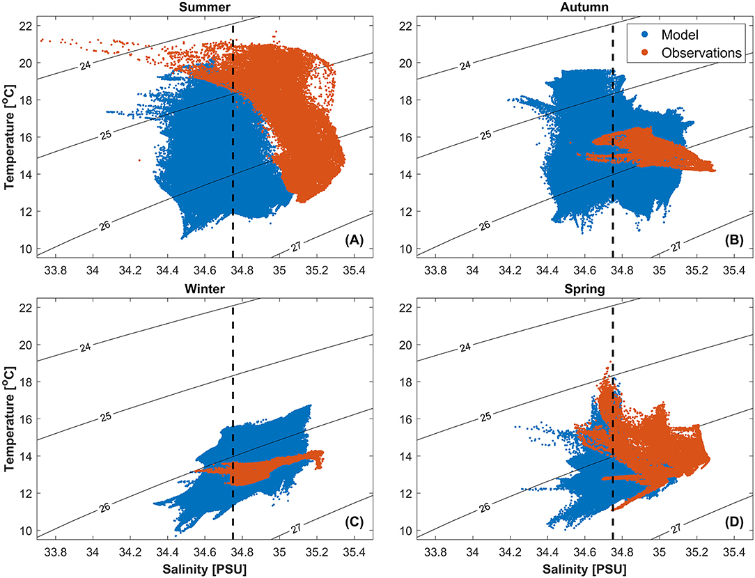
Figure 2. T-S diagram for (A) Summer, (B) Autumn, (C) Winter and (D) Spring overlaid on isopycnals for modelled results (extracted along an averaged glider track in the modelled domain) and glider observations concatenated according to their seasonal affiliation. Salinity threshold value of 34.75 psu used to detect observed LSMFs overlayed (black dashed line).

3.5. Modeled LSMFs

The modeled results reproduced persistent LSMFs throughout all seasons. For this analysis, three distinct oceanographic cases were chosen: modeled LSMF in spring 2009, modeled LSMF in spring 2011 and absence of LSMF in spring 2010 (Table 3). Analysis of the temporal and spatial scales were carried out for the two LSMF cases. The LSMF on August 28, 2011 which was in late winter and beginning of spring, will be referred to as a spring LSMF hereafter. Salinity gradients throughout the entire simulation period were generally lower in the modeled results compared to observations (Figure 2). Thus, a lower salinity threshold of ⩽ 34.6 psu was used to identify LSMFs from the modeled results. The scenario with no LSMF in Greater Cook Strait was included in the study for a dynamical comparison.

TABLE 3

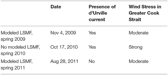
Table 3. Three cases chosen from modeled results for analysis during presence and absence of modeled LSMFs.

Wavelet coherence was used to quantify coherence between wind stress and LSMFs near Farewell Spit. V-momentum component of surface wind stress was used for this analysis as it is along the direction of advection of LSMFs out of Golden Bay. The wavelet transform analysis was performed following the method described by Grinsted et al. (2004) and the wavelet transform coherence software is available at http://www.pol.ac.uk/home/research/waveletcoherence/. We also followed their choice of Morlet wavelet which is appropriate when using wavelets for feature extraction purposes, because it is reasonably localized in both time and frequency.

3.6. Stratification and Density Stability Ratio

Density stratification (or degree of stability) was characterized by buoyancy frequency squared $N^2=\frac{-g}{{\rho }_0}\frac{\partial \rho }{\partial z}$, where g = 9.81 m s⁻² is the acceleration due to gravity, ρ₀= 1027 kg m⁻³ is the reference density and ρ is the potential density. Turner angle, Tu was calculated to quantify the relative importance of temperature and salinity gradients for density gradients. Tu also identifies where water column stability is undermined by double diffusion. Tu is calculated from density ratio as follows:

$\begin{array}{ll}\begin{array}{l}{R}_{\rho }=\frac{\alpha \Delta T}{\beta \Delta S}\\ \text{ Tu}={\text{tan}}^{-1}(R_{\rho })\end{array}& (1)\end{array}$

where $\alpha =-\frac{1}{{\rho }_0}\frac{\partial \rho }{\partial T}$ is the thermal expansion coefficient and $\beta =\frac{1}{{\rho }_0}\frac{\partial \rho }{\partial S}$ is the haline contraction coefficient calculated at the measured T and S, respectively. The horizontal differences ΔT and ΔS are taken across the spatial interval between consecutive glider profiles for observations (variable metric distance) and between consecutive grid points for modeled results (1 km). The density ratio was calculated by differencing the binned data, and since the horizontal differencing was 0.1–1 km for glider observations and 1 km for modeled results, the resolved wavelengths were 0.2–2 and 2 km, respectively. |Tu| < $\frac{\pi }{4}$ indicates that salinity gradients are more important than temperature gradients in setting the density gradient. |Tu| > $\frac{\pi }{4}$ indicate the opposite, i.e., temperature gradients dominate the density gradient.

Analysis for this study was performed with Tu following the studies of Rudnick and Martin (2002) and Jaeger and Mahadevan (2018) who highlighted the advantages of using Tu over R_ρ. Unlike R_ρ, Tu is confined to a finite range (−π/2 ⩽ Tu ⩽ π/2). Another advantage of using Tu is that temperature and salinity dominated regions occupy domains of equal size on the Tu axis. The distribution of density ratio in the water column was examined using the normalized probability density function of Tu based on the approach used by Rudnick and Martin (2002).

3.7. Submesoscale Sensitivity of LSMFs

Along-tracks lateral buoyancy gradient (M²) was calculated as the difference between mixed layer buoyancy (b) on consecutive profiles for observed LSMFs. M² was also calculated for modeled LSMFs, but the difference between mixed layer buoyancy was calculated on consecutive grid points (horizontal spacing = 1 km). The mixed layer buoyancy is calculated as follows:

$\begin{array}{ll}b=g(1-\frac{\rho }{{\rho }_0})& (2)\end{array}$

where g is acceleration due to gravity,ρ₀ is reference density as defined in section 3.6 and ρ is the mixed layer density. Balanced Richardson number (Ri_b) was then calculated as follows:

$\begin{array}{ll}R{i}_b=\frac{N^2{f}^2}{M^4}& (3)\end{array}$

where f is the coriolis parameter, N² is vertical stratification and M² is the horizontal buoyancy gradient. Ri_b was used as a criterion to indicate that submesoscale processes may occur, following the approach by Thomas et al. (2013) and Biddle and Swart (2020). Ri_b is a measure of horizontal buoyancy gradient against the vertical stratification. As Ri_b approaches unity, or is smaller than 1 (when horizontal buoyancy gradients are larger than vertical buoyancy gradients), it indicates that submesoscale processes may occur (Thomas et al., 2013; Biddle and Swart, 2020), resulting in mixed layer baroclinic instabilities and fronts.

3.8. Determining the Mixed Layer Depth and Mixing Power From Wind

Mixed layer depths (MLD) of the region were computed from temperature and salinity profiles for modelled results and glider observations. MLD was defined as the depth at which density becomes 0.125 kg.m⁻³ denser than the surface value (0 m for modeled results and mean of top 5 m for glider observations). This definition generally coincides with the seasonal thermocline (Chiswell, 2011) and was introduced by Chiswell et al. (2013) while investigating the climatology of chlorophyll a in the southwest Pacific Ocean. Mixing power from wind was calculated as in (4) to determine when wind becomes the dominant mixing mechanism.

The power per unit area generated by the wind stress on the sea surface is:

$\begin{array}{ll}\frac{\partial {\Phi }_w}{\partial t}=\tau u^{*}& (4)\end{array}$

where, τ is the surface wind stress and u^* is the wind shear velocity at the ocean surface and equals:

$\begin{array}{ll}{u}^{*}=\sqrt{\frac{\tau }{\rho }}& (5)\end{array}$

4. Ocean Glider Results

4.1. Detection and Characteristics of Observed LSMFs

Observations from seven glider surveys completed from 2015 to 2018 have shown 22 persistent LSMFs (Figure 3). Seven LSMFs were observed north of Farewell Spit, seven in Greater Cook Strait, one near Stephens Island and seven in Golden and Tasman Bays (Table 2). LSMFs were observed in all seasons (Figure 3). Glider survey in spring-summer 2015 was the only one during which no LSMFs were observed (Figures 3A,B). LSMFs were observed within the top 50 m of the water column profiles, indicating that they are features that are not restricted to the surface. The highest range in temperature and salinity were observed in summer 2018 when salinity values of < 34.4 psu and temperatures of > 20°C were recorded. More LSMFs were observed during the glider survey in summer 2018 in Golden and Tasman Bays (Figures 3M,N). Note that a glider could be sampling the edge, the width or circling around the LSMF depending on currents and tides.

FIGURE 3

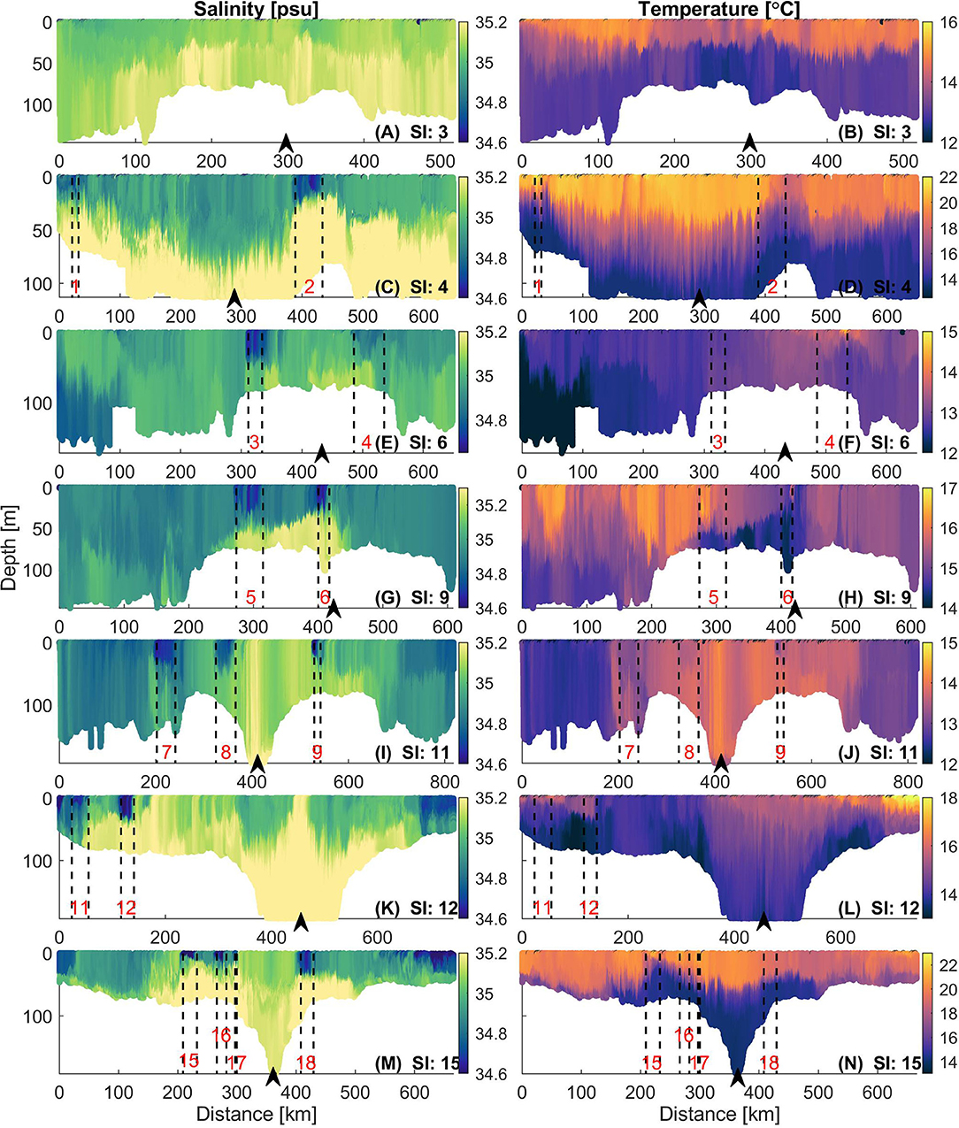
Figure 3. Salinity and temperature transects for seven glider surveys in Greater Cook Strait. SI: Glider Survey Index consistent with Tables 1, 2; (A,B) SI 3, (C,D) SI 4, (E,F) SI 6, (G,H) SI 9, (I,J) SI 11, (K,L) SI 12 and (M,N) SI 15. In each glider survey, the glider goes from east to west and back; black arrow in each transect indicates westernmost turn-around point of glider for each survey. LSMFs observed in Greater Cook Strait, north of Farewell Spit and near Stephen Island (15 out of 22 LSMFs) are highlighted by black dashed lines and numbered in red for each transect. Geographical locations of LSMFs are highlighted in blue circles on Figure 1B. The LSMF numbering is consistent with Table 2. Note: Colorscales for temperature transects were adjusted to resolve temperature gradients in each survey due to high seasonal variability.

A typical LSMF in Greater Cook Strait (LSMF 12, Table 2) had a width < 25 km, vertical extent shallower than 30 m, occupying ~ 30% of the entire water column, and was sampled for T < 20 h. Vertical differences in salinity and temperature of ΔS = 0.64 psu and ΔT = 2.32°C were observed for LSMF 12 (Figures 3K,L). Maximum differences were observed during summer 2018 (Figures 3M,N) with ΔS_max = 1.52 psu (LSMF 15) and ΔT_max = 6.95°C (LSMF 16). These extremes and the more frequent LSMFs are explained by atypical summer rainfall from two ex-tropical cyclones Fehi and Gita during February 2018 which caused flooding and increased discharges from the Motueka River into Tasman Bay.

4.2. Vertical and Horizontal Gradients of LSMFs During Spring

In spring, increased stratification was observed at the base of LSMFs (Figures 4A,B), with generally stronger stratification in spring 2017 (Figure 4B) compared to spring 2016 (Figure 4A). Temperature gradients were weaker in spring 2016 than in spring 2017. In the following subsections, the stability of the water column before, within and after two observed LSMFs with (Figures 3E,F) and without (Figures 3K,L) a temperature signal were investigated.

FIGURE 4

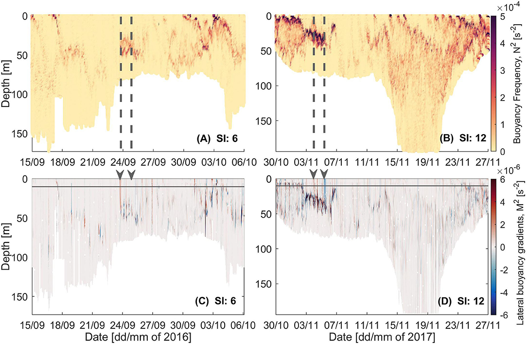
Figure 4. (A,B) Buoyancy frequency and (C,D) lateral buoyancy gradients for glider Survey Indexes 6 and 12. Start and end of LSMFs as sampled by glider for the two surveys denoted by (A,B) gray dashed lines and (C,D) gray arrows. Gray solid line indicates the depth to which density was interpolated horizontally across profiles with missing shallow values, due to the glider diving pattern.

4.2.1. Observed LSMF, Spring 2016: No Temperature Signal

The response of the water column stability to decreased salinity, without a temperature signal was evaluated for an observed LSMF in spring 2016 (LSMF 3 on Table 2 and Figures 3D,E). Before the glider approached the LSMF, stratification in the water column was very weak with N²≈0 s⁻² (Figure 5A); the water column was well-mixed. Tu distribution was bimodal at this stage, with its positive peak in the range π/4 to π/2, implying that temperature gradients were more important for water column stability.

FIGURE 5

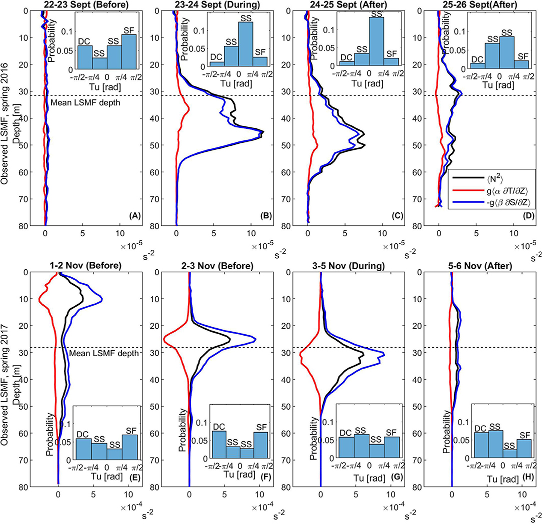
Figure 5. Vertical stratification N²(s⁻², in black), with contributions from temperature (red) and salinity (blue) before, during and after sampling observed LSMF in 2016 (top panel) and observed LSMF in spring 2017 (bottom panel). The angled brackets represent averaging over a certain number of profiles sampled before, during and after observed LSMF in 2016 (over 150 profiles) and observed LSMF in 2017 (over 250 profiles). Mean LSMF depth for each LSMF in black dashed lines. Histograms of probability density function of Turner angle, Tu for all data points (A,E,F) before, (B,G) during, and (C,D,H) after the two LSMFs. Note the different scale for N² for the two surveys. DC, Diffusive convection; SS, Statically stable; and SF, Salt fingering.

As the glider crossed the LSMF (Figures 5B,C), increased vertical stratification was observed in the subsurface layer and across the pycnocline, with a stronger haline contribution than thermal. Stratification increased sharply below the mixed layer, with the main pycnocline lying between 25 and 35 m within the LSMF. During, and 1 day after a glider crossed the LSMF, Tu distribution was predominantly in the range −π/4 to π/4, with the highest peak lying in the range 0 to π/4. This showed that salinity gradients became more important than temperature gradients in setting the density gradient during these stages. Density differences in the vertical increased from Δρ = 0.3 kg m⁻³ to Δρ = 0.5 kg m⁻³.

As the glider moved beyond the LSMF by 26 km, vertical stratification was weaker (Figure 5D). Although salinity gradients started decreasing at this stage with less data points in the range −π/4 to π/4 compared to the two previous stages (Figures 5B,C), salinity dominated vertical density gradients.

4.2.2. Observed LSMF, Spring 2017: With Temperature Signal

The LSMF observed in spring 2017 had a collocated horizontal increase in temperature of ΔT = 1.4°C (observed LSMF on Figures 3K,L). This collocated signal was also observed with satellite SST (not shown). Stratification in the water column before the LSMF was strong in the upper 18 m, and had contributions from both thermal and saline variations (Figure 5E). Tu distribution was bimodal at this stage, with its positive peak in the range π/4 to π/2 and negative peak in the range −π/2 to −π/4. This implies that temperature gradients were more important in setting the density gradient.

As the glider approached the LSMF (Figure 5F), stratification in the water column had both saline and thermal contributions as in the previous stage. Stronger stratification occurred near the mean depth of the LSMF, and the upper 18 m was well-mixed with N²≈0 s⁻². However, even though there was an increase in the saline contribution term toward N², Tu distribution showed that temperature gradients were still more important than salinity gradients at this stage. Tu distribution was bimodal, with its positive peak in the range π/4 to π/2 and negative peak in the range −π/2 to −π/4.

As the glider crossed the LSMF (Figure 5G), strong stratification persisted with both saline and thermal contributions. Strong stratification at this stage occurred below the base of the LSMF, and the upper 22 m was well-mixed with N²≈0 s⁻². The mixed layer depth was slightly deeper at this stage. Tu distribution showed that salinity gradients became more important than temperature gradients, with its highest peak in the range −π/4 to 0. However, the other two high peaks (with slightly fewer data points in each averaging bin) indicated that temperature gradients still had a strong contribution in setting the density gradient. Density differences in the vertical increased from Δρ = 0.5 kg m⁻³ to Δρ = 1.1 kg m⁻³, in the presence of both temperature and salinity gradients.

For the next 24 h, there was a decrease in stratification due to a decrease in both salinity and temperature gradients as the glider continued its track past the LSMF (Figure 5H). Even though salinity gradients had a strong contribution in setting the density gradient (highest peak in the range −π/4 to 0), other peaks show that temperature gradients also have a contribution towards the density gradient.

4.2.3. Observed Horizontal Gradients and Submesoscale Sensitivity

Mixed layer baroclinic instabilities and fronts evolve at the mixed layer Rossby radius of deformation, L = NH/f with typical length scales of L ~ 1–10 km, where N is the buoyancy frequency in the mixed layer, and H is the mixed layer depth. Mixed layer rossby radius of deformation of L ≈ 0.1–1.6 km was evaluated for the two glider surveys 6 (spring 2016) and 12 (spring 2017) during which LSMF case studies were investigated.

Observed lateral buoyancy gradients (M²) in the range O(⁻⁹) to O(⁻⁶) s⁻² were evaluated for both glider surveys (Figures 4C,D). At the observed LSMF fronts, lateral buoyancy gradients were ~ 2 × 10⁻⁶s⁻² and ~ 3 × 10⁻⁶s⁻² were in spring 2016 and spring 2017, respectively (Figures 4C,D). Thompson et al. (2016) and Du Plessis et al. (2019) have reported that gradients in this order can be observed in regions of strong horizontal gradients. Ri_b was <1 for at least 10 consecutive profiles at the front of observed LSMF in spring 2016 and for at least five consecutive profiles at the LSMF front in spring 2017. These strong lateral gradients can result in vertical shear in the horizontal velocity that can overcome the stabilizing effect of vertical density gradients. Arising submesoscale instabilities can also deviate the geostrophic balance and support vertical velocities as large as 100 m day⁻¹ at fronts (Mahadevan, 2016).

5. Complementing Observations With Modeled Results

5.1. Comparing Glider Observations and Modeled Results

Modeled results reproduced LSMFs in Greater Cook Strait that persisted throughout all seasons and at similar spatial scales as observed by gliders. In total, 151 LSMFs were detected in the modeled period April 2, 2009 to September 2, 2012. LSMFs had lifetimes between 12 h and 11 days, with periods of up to 3 weeks with no LSMFs (triangles, Figure 6). The latter was consistent with glider observations (Glider survey index 3). Twelve hours is the lower detection limit of LSMF lifetime from model outputs because of the model resolution. Modeled results also reproduced 15 events of two concurrent LSMFs (forced by different rivers at the same time). LSMF events originating from Golden and Tasman Bays into Greater Cook Strait and their lifetimes were determined using a salinity difference of ~ 0.4 psu. As river freshwater influx was applied as interpolated annual-mean values in the model, investigation of impacts of seasonal variations in river discharge on LSMFs was beyond the scope of this study. However, irregular occurrence of LSMFs in the model (Figure 6) reveals that river discharge variability may not be the dominant generation mechanism. Other potential generation mechanisms include tides and wind. These are later discussed.

FIGURE 6

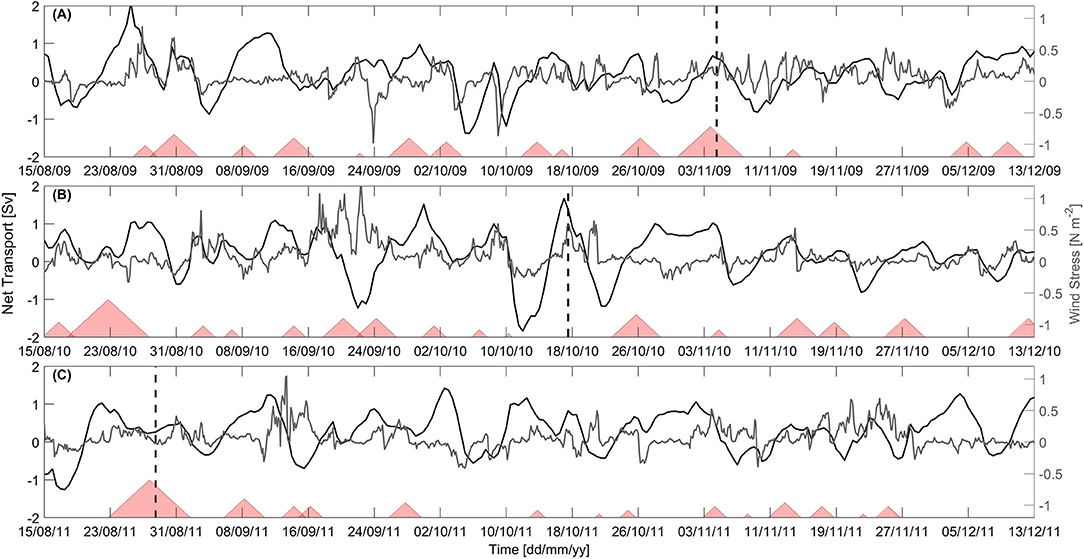
Figure 6. Detided modeled transport of the d'Urville Current in Sverdrups (Sv, black line), surface U-momentum wind stress (gray line) and occurrence of LSMFs (red triangles) in Greater Cook Strait for (A) spring 2009, (B) spring 2010, and (C) spring 2011. Transport and wind stress were averaged over the width of the d'Urville Current along transect indicated on Figure 8A. Date of the two case study LSMFs and absence of LSMF analyzed in this study overlayed as black dashed lines for (A) LSMF on November 4, 2009, (B) Absence of LSMF on October 17, 2010, and (C) LSMF on August 28, 2011. The presence of LSMFs is indicated by triangles, with LSMF duration proportional to the corresponding triangle size.

Water mass composition compared well between modeled results and observation in spring (Figure 2). Modeled ranges of salinity and temperature, ΔS_mod = 0.98 psu (μ = 34.80 psu,σ = 0.12 psu) and ΔT_mod = 8.34°C (μ = 12.78°C,σ = 0.70°C) compare well to observed ranges of ΔS_obs = 0.73 psu (μ = 35.03 psu,σ = 0.13 psu) and ΔT_obs = 8.00°C (μ = 13.74°C, σ = 1.00°C). In autumn and winter, the observed temperature ranges of ΔT_obs ~ 2°C were narrower than simulated ranges of ΔT_mod ~ 9 and ~ 7°C, respectively. In summer, although observed and modeled temperature range and mean are similar, ΔT ~ 10°C, the observed salinity range, ΔS, was wider than modeled range by ~ 0.6 psu. This is because observations in summer comprised two cyclones, which skewed the observed salinity range in summer.

During summer and spring, observations and modeled results compared well, with interannual variability captured from glider surveys resolved in numerical simulations (Figures 2A,D). However, the actual differences between modeled results and observations may be higher than shown in Figure 2 because the 12-h modeled averages smooth out subdaily variability. Moreover, modeled results used in Figure 2 spanned over periods of 3 months while glider data covered 20–35 days per mission. Observation years were different from modeled years (2015–2018 for observations and 2009–2012 for modeled results, respectively).

Ranges of both temperature and salinity were more realistic in the modeled results in spring compared to other seasons. For this reason, LSMFs from spring were chosen for comparison of modeled results and observations. While gliders provided evidence of the presence and scale of LSMFs in Greater Cook Strait for the first time, modeled results evaluation enabled a broader spatial perspective and characterization of LSMFs.

5.2. Variability of d'Urville Current

Transport variability of the d'Urville Current for 2009–2012 was analyzed across a north-south axis in Greater Cook Strait (Figure 8A). Modeled results have shown that the d'Urville Current is a semi-permanent barotropic current in Greater Cook Strait, occupying the full water column in the shallow Greater Cook Strait shelf area in most occurrences. It is highly variable in time and intensity, with frequent reversals (Figure 6).

Although maximum range of d'Urville Current transport north of Golden and Tasman Bays was found to be −2 to 2 Sv (1 Sv = 10⁶m³s⁻¹), a mean eastward flow of 0.39 Sv for the d'Urville Current was reproduced for Greater Cook Strait. Stevens (2014) resolved an estimated average volume flux of 0.25 Sv at the Cook Strait Narrows from acoustic Doppler current profilers, which he noted was smaller than previous estimates. Figure 6 shows that the d'Urville Current is highly variable in time, with positive or negative transport indicating presence of d'Urville Current in Greater Cook Strait. The d'Urville Current transport range of the modeled results used in this study is consistent with Hadfield and Stevens (2020) who reported the mean volume flux through Cook Strait as 0.42 ± 0.08 Sv from three hindcasts of currents in Cook Strait from a baroclinic, tide-resolving ocean model.

Along-d'Urville Current surface wind stress and modeled current transport were moderately correlated. Coherence squared of typically about 0.4 was evaluated between the two time series (Figure 7). The coherence well exceeds the 95% confidence limits for most periods > 1 day (Figure 7). Cross spectrum analysis between surface U-momentum wind stress and detided modeled transport of the d'Urville Current showed an in-phase relationship for periods of 2–8 days (not shown). Assessing the drivers of the d'Urville Current is beyond the scope of this study. This requires a complex modeling approach and has been investigated by Hadfield and Stevens (2020) who found that at least 87% of the variability in the subtidal transport through Cook Strait can be explained by wind (Hadfield and Stevens, 2020).

FIGURE 7

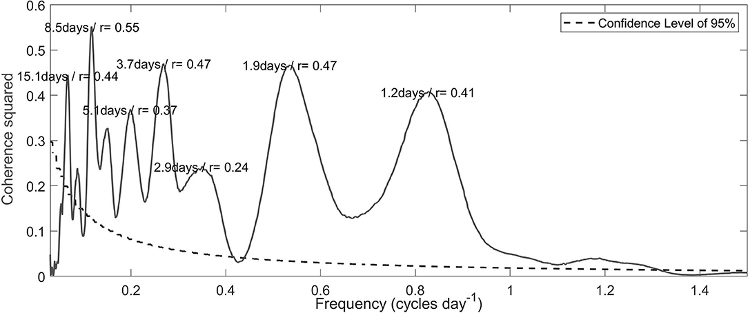
Figure 7. Cross spectrum showing coherence squared between surface U-momentum wind stress and detided modeled transport of the d'Urville Current for the entire timeseries (April 2009 to September 2012). The 95% confidence limits denoted by dashed line. Period and coherence squared values labeled for each peak.

5.3. Modeled LSMFs and Different Modes of d'Urville Current

A linear regression model between d'Urville Current transport and LSMF duration was used to investigate the link between current transport and all simulated LSMF occurrences. The model showed that with stronger transport, LSMFs have shorter lifetimes. An R² = 0.295 and p-value = 0.05 were obtained from the model, implying that 30% of LSMFs duration/occurrences could be explained by variability in currently strength. The regression analysis was therefore considered statistically significant.

Two LSMFs from spring 2009 and spring 2011 were identified from the modeled results (section 3.5) for analysis in the following sections. The criteria for selecting these two LSMFs were duration and offshore extent, strength of the d'Urville Current, wind strength, and LSMF geometry that compared well with observations. LSMFs can be sourced from rivers entering Greater Cook Strait in the form of plumes through Golden and Tasman Bays (Figures 8A,G). Modeled results revealed that detachment is a common characteristic of the plume under the condition of instability. At times, LSMFs also originated from other sources, such as from the west of Farewell Spit and from the eastern side of Greater Cook Strait near Stephens Island. This study focused on LSMFs originating from Golden and Tasman Bays due to the higher prevalence of LSMF from these two bays.

FIGURE 8

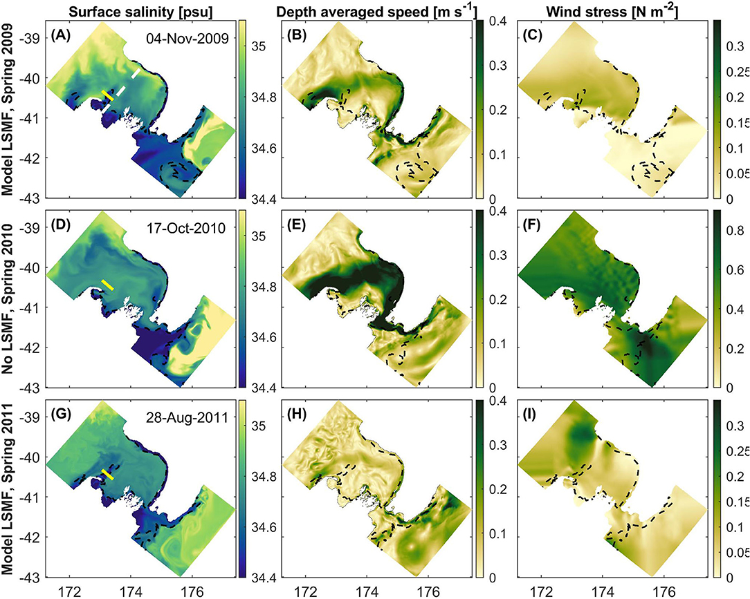
Figure 8. Map of modeled domain and modeled results of (A,D,G) surface salinity, (B,E,H) depth averaged speed, and (C,F,I) magnitude of wind stress on November 4, 2009 (top panel), October 17, 2010 (middle panel), and August 28, 2011 (bottom panel) at 18:00. White dashed line (A) is the transect defined for the calculation of d'Urville Current transport in Greater Cook Strait. 34.6 psu contour was overlayed in black dashed line in each subplot. Yellow lines in (A,G) are transects chosen to analyse the vertical structure during each the two modeled LSMFs and in (D) during the absence of a modeled LSMF. Note different colorscales used for wind stress.

Propagation of modeled LSMFs offshore was measured as the distance from midpoint between Aorere and Takaka River mouths on the coastline (Rivers 1 and 2 on Figure 1B) and the maximum location of the 34.6 psu contour offshore in a straight line from that midpoint. A straight line north-eastwards from that midpoint to the North Island coastline is 170 km. Based on LSMF case studies from modeled results shown in Figures 8A,G, the modeled LSMFs surface salinity fronts propagated ~ 75 km in 4.5 days and ~ 100 km in 6 days which gives an average advection speed of 0.2 m s⁻¹.

Modeled LSMF in November 2009 had begun advecting offshore 2 days earlier in the presence of a relatively weak d'Urville Current (0.1 Sv) and in the absence of strong southwesterly winds (wind stress <0.1 N m⁻²) in Greater Cook Strait (Figure 6A). On November 4, 2009, the modeled results reproduced a wind stress of <0.2 N m⁻² and a strengthened d'Urville Current of transport 0.7 Sv in Greater Cook Strait (Figure 6A). The modeled LSMF reached a maximum extension of 75 km offshore on that date (Figures 8A–C) before getting entrained by the d'Urville Current. The salinity difference between the LSMF and the d'Urville Current was ΔS ≈ 0.5 psu.

On October 17, 2010 18:00, a much stronger d'Urville Current of 1.4 Sv and strong southwesterly winds (wind stress > 0.7 N m⁻²) was reproduced by the model in Greater Cook Strait (Figure 6B). Salinity differences were weaker than during LSMF identified in November 2009, with ΔS <0.2 psu between the bays and the d'Urville Current (Figures 8D–F). No LSMF was reproduced by the model on this date. Salinity fronts from riverine waters reached a maximum extension of 36 km offshore on that date (Figures 8D–F).

During the modeled LSMF in spring 2011 on August 28, the d'Urville Current was relatively weak (0.2 Sv) and winds were moderate (wind stress <0.2 N m⁻²) (Figure 6C). Similar conditions had persisted for days prior and after August 28, 2011 in Greater Cook Strait (Figure 6C). The modeled LSMF reached a maximum extension of 100 km offshore in this case (Figures 8G–I).

5.4. Investigating the Role of Wind in Enhancing LSMFs Advection

Mixing power from wind ranged between O(⁻⁶) and O(⁻²) W m⁻²(Figure 9A) as calculated from equation (4). Values of mixing power were in the order O(⁻²) in the presence of strong d'Urville current and winds and was in the order O(⁻⁴) in the presence of weaker conditions.

FIGURE 9

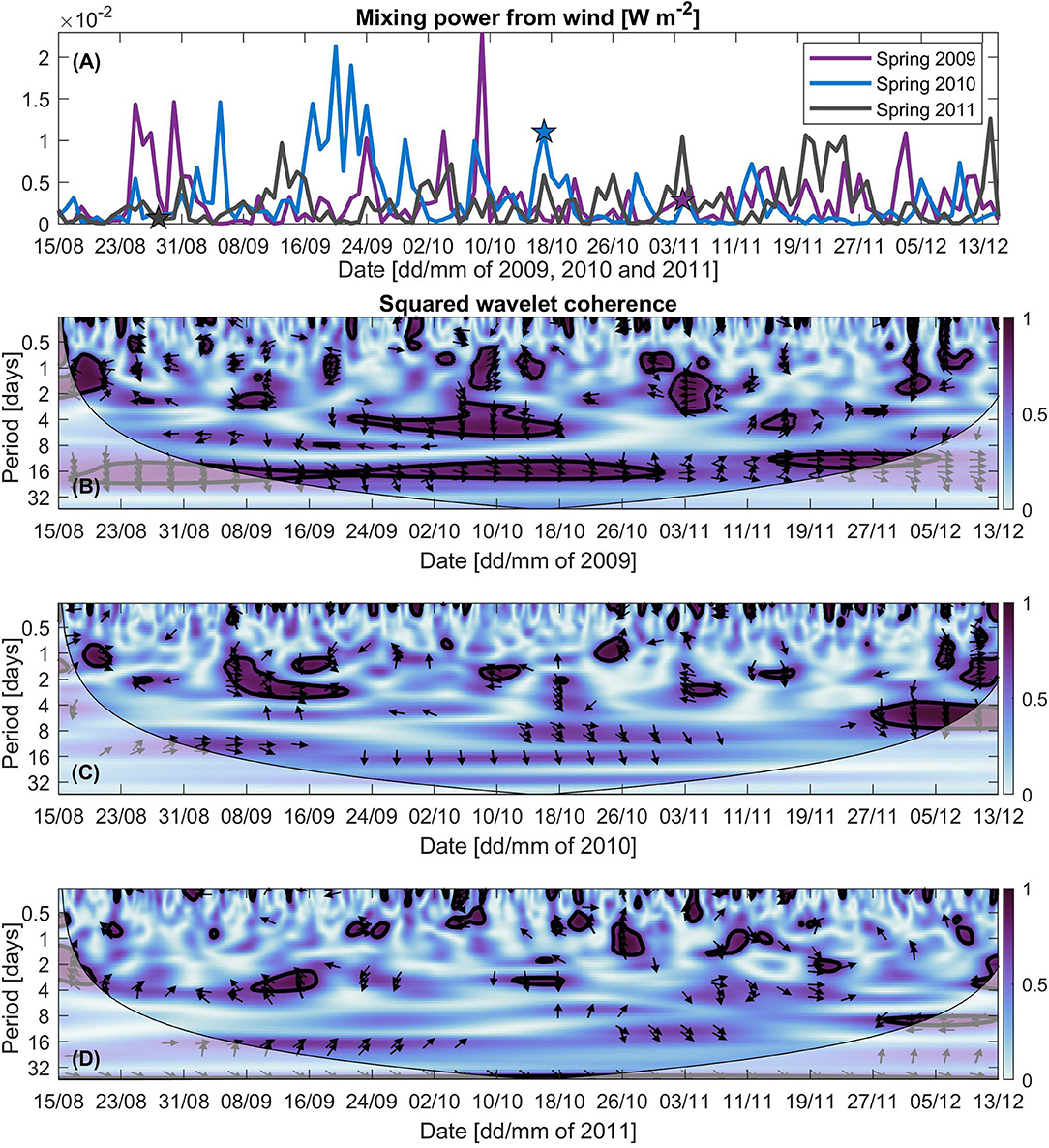
Figure 9. (A) Mixing power from wind for springs 2009 (purple), 2010 (blue), and 2011 (gray), calculated across yellow transects indicated on Figure 8. (A) Stars indicate wind mixing power on dates of analyzed modeled case studies in each spring. Time series Wavelet transform coherence squared of surface V-momentum wind stress and surface salinity near the opening of Golden Bay for springs (B) 2009, (C) 2010, and (D) 2011. The cone of influence (Torrence and Compo, 1998) where discontinuities at end points occurred because of padding with zeros and may cause distortion of the results are indicated by the lighter shade. Thick black contour indicates 95% confidence level, using red noise as background spectrum. The arrows indicate the relative phase relationship, with in-phase pointing right, anti-phase pointing left, and wind stress leading salinity by 90° pointing straight down. The time axes for each spring are consistent with those in Figure 6.

Coherence between LSMF surface wind stress and surface salinity near the oceanic boundary of Golden Bay show a mix of non-extensive significant anti-phase and in-phase relationships between the two series (Figures 9B–D). This demonstrates that wind does not always have an influence on salinity.

High coherence between wind stress and surface salinity was evident during early November 2009 when an LSMF was present (Figure 9B). This implies that winds induce the advection of low salinity water during that period as the two time series are in anti-phase over a period of 1–5 days. Significant coherence patterns were found occurring at similar periods on other dates, such as in mid-August 2009, beginning of September 2009 (Figure 9B), beginning of November 2010 (Figure 9C), and mid-September 2011 (Figure 9D). In contrast, there was a low coherence during the modeled LSMF occurring at the end of August 2011 (Figure 9D). Similar patterns was found for few other LSMFs, for example at the end of August 2009 (Figure 9B) and end of September 2010 (Figure 9C). Weak or no significant coherence with an anti-phase relationship was found on days when there is no LSMF over periods of 1–5 days, for example during the last week of September 2009 (Figure 9B), mid-October 2010 (Figure 9C), and beginning of October 2011 (Figure 9D).

High coherence was also found in spring 2009 over a longer period of 10–25 days, with an in-phase relationship (Figure 9B). This could be the d'Urville Current driven by the V-component of wind stress along the north-west coast of the South Island, bringing saltier water in the bays. At times, wind stress leads high salinity water by 90 at periods of 4–8 days, for example during mid October 2009 (Figure 9B) and beginning of December 2010 (Figure 9C). This could potentially be wind stress leading the d'Urville Current or wind-driven upwelling leading high salinity water by a phase of 90° in the region.

5.5. Vertical Structure, Stratification, and Horizontal Gradients During Modeled LSMFs

Water column stability from modeled results was evaluated for the two modeled LSMFs (Figures 10C,I) and during the absence of a modeled LSMF (Figures 10D,E). The model can reproduce LSMFs that do not have a collocated temperature signal with low salinity, however both modeled LSMFs evaluated in this study had a collocated temperature signal.

FIGURE 10

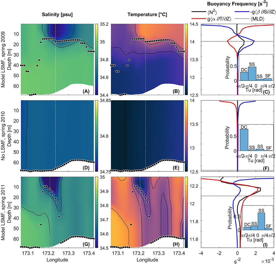
Figure 10. Vertical structure of modeled (A,D,G) salinity, (B,E,H) temperature, and (C,F,I) buoyancy frequency N² (s⁻², in black), with contributions from temperature (red) and salinity (blue) on November 4, 2009 (top panel), October 17, 2010 (middle panel), and August 28, 2011 (bottom panel) across transect indicated in Figure 8. Black dots and black dashed line indicate (A,B,D,E,G,H) MLD across entire transect, (C,I) mean MLD across width of modeled LSMFs, and (F) mean MLD across the entire transect. Buoyancy frequency plotted for 1 profile (white dashed line). (C,I) Histograms of probability density function of Turner angle, Tu for all data points across width of modeled LSMFs in spring 2009 and spring 2011, and (F) across the entire transect during the absence of a modeled LSMF. DC, Diffusive convection; SS, Statically stable; and SF, Salt fingering.

Modeled LSMF on November 4, 2009 had a vertical extent of 20–25 m, a width of ~ 20 km and was characterized by an increase in temperature (ΔT = 0.9°C) (Figures 10A,B). Maximum stratification in the water column occurred in the subsurface near the base of the LSMF, with both saline and thermal contributions (Figure 10C). Tu distribution showed that salinity gradients were more important than temperature gradients, with its highest peak in the range −π/4 to 0. The second highest peak in the range −π/2 to −π/4 indicated that temperature gradients still had a contribution in setting the density gradient. Mean MLD was 15.9 m (Figure 10C) and the mixing power from wind was 2.85 × 10⁻³W m⁻² (Figure 9A) across the width of the LSMF on this date. In the absence of an LSMF on October 17, 2010, the water column was homogenous in flows and density (Figures 10D–F). Highest peak of Tu distribution was in the range −π/2 to −π/4. Mean MLD was 63.9 m (Figure 10F) and the mixing power from wind was 1.10 × 10⁻²W m⁻² (Figure 9A).

Modeled LSMF on August 28, 2011 had a vertical extent of 30–35 m and a width of ~ 10 km. The modeled LSMF in spring 2011 was characterized by a decrease in temperature (ΔT = 0.5°C) (Figures 10F,G). Maximum stratification occurred in the subsurface (at 10–15 m) with both saline and thermal contributions (Figure 10I). Tu distribution was predominantly between 0 and π/4, indicating that salinity gradients regulated density gradients in this case. Mean MLD was 17.5 m (Figure 10I) and the mixing power from wind was 7.15 × 10⁻⁴W m⁻²(Figure 9A) across width of LSMF. The unrealistic vertical geometry of this modeled LSMF highlights one of the limitations of the model. The simulated sloping isopycnals as lower bound of the LSMF are inconsistent with the observed flat isopycnals at the base of LSMFs.

5.5.1. Modeled Horizontal Gradients and Submesoscale Sensitivity

Mixed layer rossby radius of deformation of L ≈0.1–10 km was obtained across a simulated average glider track confirming that submesoscale processes can develop in the model. However, a much smaller L range observed from glider surveys highlights the applicability of autonomous platforms to sample at scales smaller than L better than currently available models. It emphasizes the importance of sampling and modeling at high spatial resolutions of <1 km to resolve the full surface variance in density, particularly in relatively shallow mixed layer environments (leading to smaller length scales) where riverine layers prevail.

Modeled lateral buoyancy gradients along a simulated glider track were generally in the range O(⁻¹⁰) to O(⁻⁷) s⁻². Fronts of the chosen modeled LSMF investigated in this study showed lateral buoyancy gradients of ~ 7 × 10⁻⁷ s⁻² and ~ 6 × 10⁻⁷ s⁻² in spring 2009 and spring 2011, respectively. These modeled lateral buoyancy gradient values at the fronts are one order of magnitude weaker than observed gradients. Furthermore, in contrast to observations, Ri_b were > 1 at both modeled LSMF fronts (in the order of 10¹ to 10²). We attribute this difference to a mismatch between the model's fixed horizontal resolution of 1-km and the distance between glider profiles ranging from 0.1 to 1 km. This analysis demonstrates the model's inability to represent realistic vertical and horizontal gradients associated with LSMFs. The modeled density gradients are too weak (by one order of magnitude) which implies that non-linear dynamical processes associated with strong fronts and stratification are misrepresented. For this reason, we refrained from the investigation of temporal evolution of LSMF structure from the model.

6. Discussion

Occurrence of LSMFs that persist through all seasons were identified for the first time in Greater Cook Strait. We revealed that the strength of the coastal current moderates the advection of LSMFs, which in turn impact the larger scale stratification over the shelf. An observational record from seven glider surveys over a 3-years period resolved seasonal to subtidal time scales of these ephemeral LSMFs. We used salinity signals for the detection of submesoscale features and highlight the importance of salinity fields in controlling upper ocean stratification in shelf seas. Our high resolution glider observations were complemented with modeling at submesoscale-permitting resolution (horizontal spacing = 1 km) to understand the processes and mechanisms driving submesoscale variability in a shelf sea.

6.1. Effects of LSMFs on Water Column Stability

Greater Cook Strait was found to have highly variable stratification which can change from strongly stably stratified to vertically well-mixed and unstable, depending on the presence or absence of LSMFs (Figure 11 and Table 4). When LSMFs are present, the water column stabilizes. When the regional current and winds are strong, enhanced vertical mixing destabilizes the water column (Figure 11).

FIGURE 11

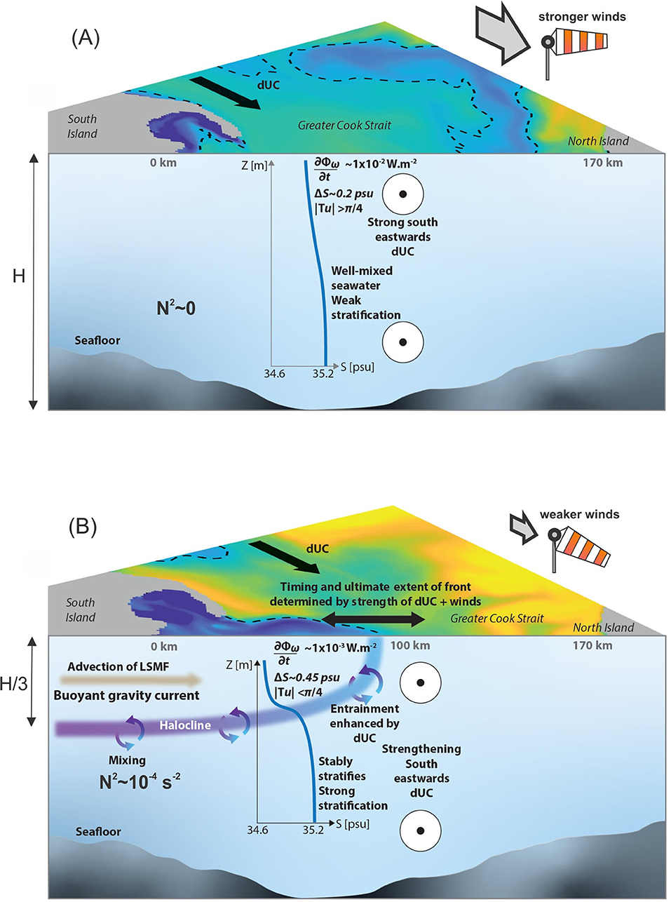
Figure 11. Schematic of Greater Cook Strait (A) in the absence of an LSMF indicating typical salinity profile, wind mixing power, and Tu in the presence of a strong wind-driven d'Urville Current and (B) in the presence of an LSMF propagating offshore, indicating typical salinity profile, wind mixing power, and Tu as it undergoes entrainment when it interacts the wind-driven d'Urville Current.

TABLE 4

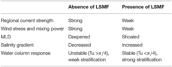
Table 4. Summary table.

The presence of strong barotropic current and winds generate a stronger mixing power by two orders of magnitude in Greater Cook Strait (Figures 4C,D). These conditions inhibit advection of LSMFs. As wind driven stirring cannot stabilize the upper ocean, an unstable ocean regime is established in the shelf region. Mixing causes temperature and salt fluxes to be almost equal. Strong mixing power from wind in shallow shelf seas can cause deepening of the MLD or mix the water column entirely. Although Tu analysis indicates that in the absence of strong salinity or temperature gradients, double diffusion is possible in Greater Cook Strait, mixing in this shallow shelf sea is mostly driven by surface stresses, such as tidal straining, wind, and diurnal cooling. This is due to its proximity to an amphidrome, high wind speeds and shallow bathymetry.

Nearly three quarters of LSMFs (73%) detected from glider observations do not have a surface temperature signal. Temperature is therefore not always a reliable indicator of LSMF and not regularly detectable by satellite SST. The inconsistency in temperature signal of river waters in Golden and Tasman Bays has been reported in previous studies by Hadfield and Sutton (1996) and Chiswell et al. (2019). The latter study found that in autumn, fresh water was associated with cooler temperatures, but in summer the fresh water was associated with warmer temperatures, which reinforced the density decrease in the bays. We found that salinity variations have a greater influence on near-surface density during an LSMF (Figures 5, 10). In the Chukchi Sea, salinity dominated the density gradient and lateral temperature and salinity gradients are non-compensating, with Tu≈0 (Timmermans and Winsor, 2013, Figure 12). Horizontal density gradients are not erased by vertical mixing in the Chukchi Sea (Timmermans and Winsor, 2013).

FIGURE 12

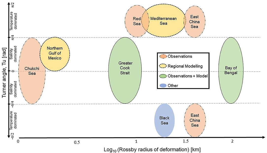
Figure 12. Oceanic regions influenced by salinity gradients, placed on the Turner angle range and respective Rossby radius of deformation. Influence on oceanic regions inferred from Timmermans and Winsor (2013) (Chukchi Sea); Barkan et al. (2017a) (Northern Gulf of Mexico); Jhugroo et al. (2020) (Greater Cook Strait—this study); Jaeger and Mahadevan (2018) (Bay of Bengal); Shi and Wei (2007) (East China Sea); Meccia et al. (2016) (Mediterranean Sea); You (2002) (Red Sea); and Kelley et al. (2003) (Black Sea).

In the presence of a weak regional current and weak winds in Greater Cook Strait, mixing power from wind is weak (Figures 8H,I, 9A). As a result, LSMFs are advected offshore, and minimal mixing occurs and the water column is able to stabilize within the feature. The locally stabilized water column and the subsequently shoaled MLD can persist for 2–3 days, even when the LSMF gets entrained by the barotropic current. The presence of an LSMF with a dominating salinity gradient creates a stable regime by increasing stratification in the subsurface and decreasing vertical and lateral mixing in the water column in this shelf sea. This study provides further evidence to MacKenzie and Adamson (2004) who reported that temporal changes in the abundance and horizontal and vertical distribution of phytoplankton biomass in Greater Cook Strait are associated with changes in water column stratification, because of variations in the magnitude of freshwater inflows.

LSMFs that also have a temperature signal have a less stable regime, as the temperature adds a compensating thermal contribution to the density gradient. However, temperature gradients were not large enough to entirely cancel the density effect of salinity and destabilize the water column. Sufficient stratification remains to suppress mixing within an LSMF with both, salinity and temperature gradients. Elsewhere, a similar regime was reported for the Columbia River plume where water column stability was significantly higher in the plume than in the surrounding ocean (Morgan et al., 2005). In the Northern Gulf of Mexico, Turner angle analysis on submesoscale-resolving modeled results showed a nearshore salinity-dominated signal and no clear compensating signal under the influence of the Mississipi-Atchafalaya River system (Barkan et al., 2017a, Figure 12).

6.2. Interaction of LSMFs With Regional Ocean Dynamics

Overall, modeled results represented the interaction of LSMFs with the regional barotropic current by reproducing drivers of the d'Urville Current and wind-induced mixing at realistic scales. The regional barotropic d'Urville Current variability is dependent on a balance between the sea level gradient and density gradient across the shelf region (Walters et al., 2001). Our results revealed that 30% of the time, the lifetime of LSMFs originating from Golden and Tasman Bays can be explained by current variability in this shelf sea. A weak regional current and weak winds allow LSMFs to advect offshore and impact water column stability at substantial distances of up to 100 km offshore from their source. In contrast, a strong regional current and strong winds inhibit offshore advection of LSMFs into the shelf region.

The presence of a weak d'Urville Current and weak winds set up conditions that favor advection of LSMFs offshore into Greater Cook Strait. When such conditions persist for at least 4 days on the shelf, LSMFs are able to extend furthest offshore (up to 100 km, Figure 8G). LSMFs under these conditions also have the longest residence time in Greater Cook Strait. When conditions are intermediate, i.e., the d'Urville Current strengthens and winds become moderate, existing LSMFs are unable to advect further onto the shelf. The LSMFs tend to be trapped at the edge of the current and entrained into coastal waters. In contrast, the presence of a strong barotropic d'Urville Current driven by strong southwesterly winds that persist for longer than 2 days in this shelf sea do not allow the advection of LSMFs offshore into Greater Cook Strait. Under these conditions, the LSMFs are constrained to the bays, because the strong d'Urville Current inhibits any further extension of the riverine waters as soon as the latter reach Farewell Spit.

Three scenarios regulate triggered LSMFs in this shelf sea: (1) weak regional current and moderate winds that last for at least 4 days create ideal conditions for the propagation of LSMFs furthest offshore. (2) Moderate regional current and moderate winds allow LSMFs to propagate into the shelf area. In this case, LSMFs can be entrained into the regional current as the current strengthens over time due to changes in wind stress and subtidal currents. (3) Strong regional current and strong winds create unfavorable conditions that prevent advection of LSMFs offshore onto the shelf region.

6.3. Generation Mechanisms of LSMFs

The observed persistent occurrence of the LSMFs, their salinity signature and their short lived nature was resolved numerically with ROMS (Figures 3, 10). Our study revealed that presence of LSMFs feeds back on the larger scale stratification of Greater Cook strait. LSMFs are generated and regulated by several mechanisms. Potential generation mechanisms of LSMFs in this shelf sea are river discharge variability, wind and tidal effects.

River discharge variability in this shelf sea is able to increase stratification in the subsurface in the order O(⁻⁴) s⁻² and cause strong lateral buoyancy gradients in the order O(⁻⁶) s⁻². Observations showed that surges of river discharges during two cyclones in summer 2018 did cause more LSMFs in Greater Cook Strait (Figure 3M). This suggests that seasonality in river flows might lead to increased LSMF occurrences for time-varying boundary conditions. Models, at times, may not represent key physical or biophysical mechanisms correctly at times (D'Ovidio et al., 2019). For example, the use of interpolated annual-mean values for each river's discharge in this study is a simplification of the natural system. However, the erratic nature of LSMF events in the model suggests that variability in river discharge is not the only cause of their advection into Greater Cook Strait.

The role of wind in enhancing LSMF generation was investigated in this study. Coherence between wind stress and salinity showed that wind can enhance the advection of LSMFs out of the bays (Figures 9B–D). This was evident for 38% of the time in spring. Recently Chiswell et al. (2019) confirmed that mean velocity in Golden and Tasman Bays is weak and circulation is a balance between wind and tidal flows. Previous studies focusing on the circulation in Golden and Tasman Bays, and Greater Cook Strait and its implication on river plume behavior (Heath, 1976; Tuckey et al., 2006; Chiswell et al., 2019), have suggested that residual flows move northwards. Typically, anticyclonic flows occur in the south of Tasman and Golden Bays, and a cyclonic flow in the north of Golden Bay. Mean near-surface velocity is generally out of each bay, with a stronger outflow along Farewell Spit in Golden Bay and near Stephen Island in Tasman Bay, which are the pathways of most triggered LSMFs. This implies that wind plays a role in enhancing LSMFs advection further offshore once residual flows have advected the LSMF out of the coastal bays.

LSMFs are advected out of the bays by a combination of river water saturation in the bays, residual northward tidal flows, and strong northwards wind in the bays. To further investigate the potential generation mechanisms, higher resolution simulations must be combined with time-varying forcing of river flow. Additional glider surveys that capture extreme events over all seasons would also enable us to identify if there is a period most favorable to mixed layer instability development.

6.4. Implications of LSMFs for Shelf Systems

Greater Cook Strait is regulated by interactions between barotropic and baroclinic processes. The coastal current is barotropic and wind-modulated; submesoscale features induce baroclinic instabilities via salinity-controlled density gradients. We found that LSMFs force lateral density gradients that in turn fuel mixed layer baroclinic instabilities in spring. The Bay of Bengal, northern Gulf of Mexico (under the influence of Mississipi-Atchalafaya river system), Chukchi Sea and north of the Amazon River are some examples of salinity-controlled shelf seas that show similar responses (Figure 12). Heavy monsoon rains and run-off can impact water column stability on shorter time scales (Jaeger and Mahadevan, 2018). Resulting stratification values on the order of 10⁻⁴s⁻² (similar to Greater Cook Strait, Figures 4A,B) caused by strong salinity gradients in the subsurface were reported for the Bay of Bengal by Jaeger and Mahadevan (2018) and Ramachandran et al. (2018). The significance of salinity was highlighted for interpreting SST in regions which are salinity-controlled, where temperature fronts can be oppositely oriented to density fronts, and cold filaments can represent increased surface stratification rather than deeper mixed layers.

Baroclinic instabilities induced by LSMFs develop at the submesoscale and work to reduce mixed-layer depth, increase vertical density stratification and decrease vertical diapycnal mixing. The LSMFs create fronts at the submesoscale that form, move and dissipate continuously—they are not in a steady-state balance between forcing and dissipation at a fixed location. Thomas et al. (2008) have shown that these fronts have associated cross-frontal secondary circulations that are generally confined to the vertically well-mixed upper layer of the ocean. Moreover, various studies have shown that the energy carried by submesoscale features can be converted to kinetic energy by mixed layer instability (Brannigan et al., 2015; Buckingham et al., 2016; Callies et al., 2016). Instabilities created by LSMFs in shelf seas may also have implications for mixing and transport of nutrients and phytoplankton. The submesoscale responses of these instabilities can have consequences on the residence time of phytoplankton in the euphotic zone and as a result, affect growth rates, biomasses, biogeochemical fluxes, and community structure, in contrast to mesoscale stirring (Lévy et al., 2018). Variability in water column stability in shelf seas can have implications not only for primary production (Iida et al., 2012), but also for higher trophic levels (Coyle et al., 2008). Although we did not show the biological responses of LSMFs in this study, our findings suggest that submesoscale processes that locally influence water column stability and MLD, may have important biological implications through mixing.

In summary, salinity-dominated submesoscale features in shelf seas and their role in stabilizing upper layer stratification were revealed by glider observations in this study. The offshore advection and lifetime of these submesoscale features were found to be modulated by the strength of a coastal barotropic current. Turner angle was used to indicate changes into stable stratification due to salinity-dominated density signals in the presence of LSMFs. Finally, we showed that stable stratification causes shoaling of the mixed layer depth, inhibiting mixing locally. Baroclinic instabilities induced by these features can have implications for mixing of nutrients and phytoplankton in shelf seas. Further development of this work will look at how seasonal differences affect the impacts of these small scale features and their biological response in this New Zealand shelf sea.

Data Availability Statement

Glider data publicly available on SEANOE (O'Callaghan and Elliott, 2020). Model runs have been carried out on the NeSI supercomputer. Requests for access to model input and output datasets should be made to the corresponding author and are welcomed, but there are issues with the inclusion of some proprietary data and the large file sizes. We are currently exploring procedures for publishing model-output datasets.

Author Contributions

KJ, JO'C, and CS contributed to the conception and design of the study. MH and HM contributed to the regional model. FE, JO'C, and KJ contributed to the glider-related field work, maintenance, piloting, and data processing. KJ wrote the first draft of the manuscript. JO'C, CS, and HM contributed to manuscript revision. All authors read and approved the submitted version.

Conflict of Interest

The authors declare that the research was conducted in the absence of any commercial or financial relationships that could be construed as a potential conflict of interest.

Acknowledgments

This study was part of the Phase I Sustainable Seas National Science Challenge. We thank NIWA Coasts and Oceans SSIF for funding, and acknowledge the contribution of New Zealand eScience Infrastructure (NeSI) to the ROMS modeling used in this research. Three-hourly winds from the MetOcean Solutions Ltd Hau Moana hindcast was sourced from the Moana Project, www.moanaproject.org, funded by the New Zealand Ministry of Business Innovation and Employment, contract number METO1801. We also acknowledge the help of Nelson fishing charters in glider deployments and recoveries. We are grateful for the constructive comments made by the three reviewers, which helped to improve the manuscript. Lastly, KJ thanks Stefan Jendersie, Charine Collins, and Rafael Santana for inputs and discussions.

References

Barkan, R., McWilliams, J. C., Molemaker, M. J., Choi, J., Srinivasan, K., Shchepetkin, A. F., et al. (2017a). Submesoscale dynamics in the northern Gulf of Mexico. Part II: temperature-salinity relations and cross-shelf transport processes. J. Phys. Oceanogr. 47, 2347–2360. doi: 10.1175/JPO-D-17-0040.1

CrossRef Full Text | Google Scholar

Barkan, R., McWilliams, J. C., Shchepetkin, A. F., Molemaker, M. J., Renault, L., Bracco, A., et al. (2017b). Submesoscale dynamics in the northern Gulf of Mexico. Part I: regional and seasonal characterization and the role of river outflow. J. Phys. Oceanogr. 47, 2325–2346. doi: 10.1175/JPO-D-17-0035.1

CrossRef Full Text | Google Scholar

Barkan, R., Winters, K. B., and Llewellyn Smith, S. G. (2015). Energy cascades and loss of balance in a reentrant channel forced by wind stress and buoyancy fluxes. J. Phys. Oceanogr. 45, 272–293. doi: 10.1175/JPO-D-14-0068.1

CrossRef Full Text | Google Scholar

Biddle, L., and Swart, S. (2020). The observed seasonal cycle of submesoscale processes in the Antarctic marginal ice zone. J. Geophys. Res. Oceans 47, 1–19. doi: 10.1029/2019JC015587

CrossRef Full Text | Google Scholar

Biggs, B. J., Duncan, M. J., Jowett, I. G., Quinn, J. M., Hickey, C. W., Davies-Colley, R. J., et al. (1990). Ecological characterisation, classification, and modelling of New Zealand rivers: an introduction and synthesis. N. Zeal. J. Mar. Freshw. Res. 24, 277–304. doi: 10.1080/00288330.1990.9516426

CrossRef Full Text | Google Scholar

Boccaletti, G., Ferrari, R., and Fox-Kemper, B. (2007). Mixed layer instabilities and restratification. J. Phys. Oceanogr. 37, 2228–2250. doi: 10.1175/JPO3101.1

CrossRef Full Text | Google Scholar

Brannigan, L., Marshall, D. P., Naveira-Garabato, A., and Nurser, A. G. (2015). The seasonal cycle of submesoscale flows. Ocean Model. 92, 69–84. doi: 10.1016/j.ocemod.2015.05.002

CrossRef Full Text | Google Scholar

Buckingham, C. E., Naveira Garabato, A. C., Thompson, A. F., Brannigan, L., Lazar, A., Marshall, D. P., et al. (2016). Seasonality of submesoscale flows in the ocean surface boundary layer. Geophys. Res. Lett. 43, 2118–2126. doi: 10.1002/2016GL068009

CrossRef Full Text | Google Scholar

Cahill, M. L., Middleton, J. H., and Stanton, B. R. (1991). Coastal-trapped waves on the west coast of South Island, New Zealand. J. Phys. Oceanogr. 21, 541–557. doi: 10.1175/1520-0485(1991)021<0541:CTWOTW>2.0.CO;2

CrossRef Full Text | Google Scholar

Callies, J., Ferrari, R., Klymak, J. M., and Gula, J. (2015). Seasonality in submesoscale turbulence. Nat. Commun. 6:6862. doi: 10.1038/ncomms7862

PubMed Abstract | CrossRef Full Text | Google Scholar

Callies, J., Flierl, G., Ferrari, R., and Fox-Kemper, B. (2016). The role of mixed-layer instabilities in submesoscale turbulence. J. Fluid Mech. 788, 5–41. doi: 10.1017/jfm.2015.700

CrossRef Full Text | Google Scholar

Capet, X., McWilliams, J. C., Molemaker, M. J., and Shchepetkin, A. (2008). Mesoscale to submesoscale transition in the California Current System. Part I: flow structure, eddy flux, and observational tests. J. Phys. Oceanogr. 38, 29–43. doi: 10.1175/2007JPO3671.1

CrossRef Full Text | Google Scholar

Chen, C., Xue, P., Ding, P., Beardsley, R., Xu, Q., Mao, X., et al. (2008). Physical mechanisms for the offshore detachment of the Changjiang Diluted Water in the East China Sea. J. Geophys. Res. Oceans 113:C02002. doi: 10.1029/2006JC003994

CrossRef Full Text | Google Scholar

Chiswell, S. M. (2011). Annual cycles and spring blooms in phytoplankton: don't abandon Sverdrup completely. Mar. Ecol. Prog. Ser. 443, 39–50. doi: 10.3354/meps09453

CrossRef Full Text | Google Scholar

Chiswell, S. M., Bostock, H. C., Sutton, P. J., and Williams, M. J. (2015). Physical oceanography of the deep seas around New Zealand: a review. N. Zeal. J. Mar. Freshw. Res. 49, 286–317. doi: 10.1080/00288330.2014.992918

CrossRef Full Text | Google Scholar

Chiswell, S. M., Bradford-Grieve, J., Hadfield, M. G., and Kennan, S. C. (2013). Climatology of surface chlorophyll A, autumn-winter and spring blooms in the southwest Pacific Ocean. J. Geophys. Res. Oceans 118, 1003–1018. doi: 10.1002/jgrc.20088

CrossRef Full Text | Google Scholar

Chiswell, S. M., Stevens, C. L., Macdonald, H. S., Grant, B. S., and Price, O. (2019). Circulation in Tasman-Golden bays and Greater Cook Strait, New Zealand. N. Zeal. J. Mar. Freshw. Res. 1–26. doi: 10.1080/00288330.2019.1698622

CrossRef Full Text | Google Scholar

Chiswell, S. M., Zeldis, J. R., Hadfield, M. G., and Pinkerton, M. H. (2016). Wind-driven upwelling and surface chlorophyll blooms in Greater Cook Strait. N. Zeal. J. Mar. Freshw. Res. 51, 1–25. doi: 10.1080/00288330.2016.1260606

CrossRef Full Text | Google Scholar

Cornelisen, C. D., Gillespie, P. A., Kirs, M., Young, R. G., Forrest, R. W., Barter, P. J., et al. (2011). Motueka River plume facilitates transport of ruminant faecal contaminants into shellfish growing waters, Tasman Bay, New Zealand. N. Zeal. J. Mar. Freshw. Res. 45, 477–495. doi: 10.1080/00288330.2011.587822

CrossRef Full Text | Google Scholar

Coyle, K. O., Pinchuk, A. I., Eisner, L. B., and Napp, J. M. (2008). Zooplankton species composition, abundance and biomass on the eastern Bering Sea shelf during summer: the potential role of water-column stability and nutrients in structuring the zooplankton community. Deep Sea Res. II Top. Stud. Oceanogr. 55, 1775–1791. doi: 10.1016/j.dsr2.2008.04.029

CrossRef Full Text | Google Scholar

D'Asaro, E., Lee, C., Rainville, L., Harcourt, R., and Thomas, L. (2011). Enhanced turbulence and energy dissipation at ocean fronts. Science 332, 318–322. doi: 10.1126/science.1201515

PubMed Abstract | CrossRef Full Text | Google Scholar

Dauhajre, D. P., McWilliams, J. C., and Uchiyama, Y. (2017). Submesoscale coherent structures on the continental shelf. J. Phys. Oceanogr. 47, 2949–2976. doi: 10.1175/JPO-D-16-0270.1

CrossRef Full Text | Google Scholar

D'Ovidio, F., Pascual, A., Wang, J., Doglioli, A., Jing, Z., Moreau, S., et al. (2019). Frontiers in fine-scale in situ studies: opportunities during the swot fast sampling phase. Front. Mar. Sci. 6:168. doi: 10.3389/fmars.2019.00168

CrossRef Full Text | Google Scholar

Du Plessis, M., Swart, S., Ansorge, I. J., Mahadevan, A., and Thompson, A. F. (2019). Southern Ocean seasonal restratification delayed by submesoscale wind-front interactions. J. Phys. Oceanogr. 49, 1035–1053. doi: 10.1175/JPO-D-18-0136.1

CrossRef Full Text | Google Scholar

Fox-Kemper, B., Ferrari, R., and Hallberg, R. (2008). Parameterization of mixed layer eddies. Part I: theory and diagnosis. J. Phys. Oceanogr. 38, 1145–1165. doi: 10.1175/2007JPO3792.1

CrossRef Full Text | Google Scholar

Garau, B., Ruiz, S., Zhang, W. G., Pascual, A., Heslop, E., Kerfoot, J., et al. (2011). Thermal lag correction on slocum ctd glider data. J. Atmos. Ocean. Technol. 28, 1065–1071. doi: 10.1175/JTECH-D-10-05030.1

CrossRef Full Text | Google Scholar

Grinsted, A., Moore, J. C., and Jevrejeva, S. (2004). Application of the cross wavelet transform and wavelet coherence to geophysical time series. Nonlin. Process. Geophys. 11, 561–566. doi: 10.5194/npg-11-561-2004

CrossRef Full Text | Google Scholar

Gula, J., Molemaker, M. J., and McWilliams, J. C. (2014). Submesoscale cold filaments in the Gulf Stream. J. Phys. Oceanogr. 44, 2617–2643. doi: 10.1175/JPO-D-14-0029.1

CrossRef Full Text | Google Scholar

Hadfield, M. G., and Stevens, C. L. (2020). A modelling synthesis of the volume flux through Cook Strait. N. Zeal. J. Freshw. Mar. Res. 1–29. doi: 10.1080/00288330.2020.1784963

CrossRef Full Text | Google Scholar

Hadfield, M. G., and Sutton, P. (1996). Tidal flushing in a bay used for mussel farming. Seafood N. Zeal. 4, 45–46.

Google Scholar

Haney, S., Fox-Kemper, B., Julien, K., and Webb, A. (2015). Symmetric and geostrophic instabilities in the wave-forced ocean mixed layer. J. Phys. Oceanogr. 45, 3033–3056. doi: 10.1175/JPO-D-15-0044.1

CrossRef Full Text | Google Scholar

Harris, T. F. W. (1990). Greater Cook Strait: Form and Flow. Wellington: DSIR Marine and Freshwater.

Google Scholar

Heath, R. A. (1976). Circulation in Tasman Bay. N. Zeal. J. Mar. Freshw. Res. 10, 469–483. doi: 10.1080/00288330.1976.9515630

CrossRef Full Text | Google Scholar

Heath, R. R., and Gilmour, A. E. (1987). Flow and hydrological variability in the Kahurangi plume off north-west South Island, New Zealand. N. Zeal. J. Mar. Freshw. Res. 21, 125–139. doi: 10.1080/00288330.1987.9516207

CrossRef Full Text | Google Scholar

Hetland, R. D. (2017). Suppression of baroclinic instabilities in buoyancy-driven flow over sloping bathymetry. J. Phys. Oceanogr. 47, 49–68. doi: 10.1175/JPO-D-15-0240.1

CrossRef Full Text | Google Scholar

Iida, T., Mizobata, K., and Saitoh, S.-I. (2012). Interannual variability of coccolithophore Emiliania huxleyi blooms in response to changes in water column stability in the eastern Bering Sea. Cont. Shelf Res. 34, 7–17. doi: 10.1016/j.csr.2011.11.007

CrossRef Full Text | Google Scholar

Jaeger, G. S., and Mahadevan, A. (2018). Submesoscale-selective compensation of fronts in a salinity-stratified ocean. Sci. Adv. 4:e1701504. doi: 10.1126/sciadv.1701504

PubMed Abstract | CrossRef Full Text | Google Scholar

Jhugroo, K., O'Callaghan, J., Stevens, C., Macdonald, H., Elliott, F., and Hadfield, M. (2020). Spatial structure of low salinity submesoscale features and their interactions with a coastal current. Front. Mar. Sci. 7:557360. doi: 10.3389/fmars.2020.557360

CrossRef Full Text | Google Scholar

Johnson, G. C., Schmidtko, S., and Lyman, J. M. (2012). Relative contributions of temperature and salinity to seasonal mixed layer density changes and horizontal density gradients. J. Geophys. Res. Oceans 117:C04015. doi: 10.1029/2011JC007651

CrossRef Full Text | Google Scholar

Kalnay, E., Kanamitsu, M., Kistler, R., Collins, W., Deaven, D., Gandin, L., et al. (1996). The NCEP/NCAR 40-year reanalysis project. Bull. Am. Meteorol. Soc. 77, 437–472. doi: 10.1175/1520-0477(1996)077<0437:TNYRP>2.0.CO;2

CrossRef Full Text | Google Scholar

Kelley, D., Fernando, H., Gargett, A., Tanny, J., and Özsoy, E. (2003). The diffusive regime of double-diffusive convection. Prog. Oceanogr. 56, 461–481. doi: 10.1016/S0079-6611(03)00026-0

CrossRef Full Text | Google Scholar

Lévy, M., Ferrari, R., Franks, P. J. S., Martin, A. P., and Riviere, P. (2012). Bringing physics to life at the submesoscale. Geophys. Res. Lett. 39:L14602. doi: 10.1029/2012GL052756

CrossRef Full Text | Google Scholar

Lévy, M., Franks, P. J., and Smith, K. S. (2018). The role of submesoscale currents in structuring marine ecosystems. Nat. Commun. 9:4758. doi: 10.1038/s41467-018-07059-3

PubMed Abstract | CrossRef Full Text | Google Scholar

Luo, H., Bracco, A., Cardona, Y., and McWilliams, J. C. (2016). Submesoscale circulation in the northern Gulf of Mexico: surface processes and the impact of the freshwater river input. Ocean Model. 101, 68–82. doi: 10.1016/j.ocemod.2016.03.003

CrossRef Full Text | Google Scholar

MacKenzie, L., and Adamson, J. (2004). Water column stratification and the spatial and temporal distribution of phytoplankton biomass in Tasman Bay, New Zealand: implications for aquaculture. N. Zeal. J. Mar. Freshw. Res. 38, 705–728. doi: 10.1080/00288330.2004.9517271

CrossRef Full Text | Google Scholar

MacKinnon, J. A., Nash, J. D., Alford, M. H., Lucas, A. J., Mickett, J. B., Shroyer, E. L., et al. (2016). A tale of two spicy seas. Oceanography 29, 50–61. doi: 10.5670/oceanog.2016.38

CrossRef Full Text | Google Scholar

Mahadevan, A. (2016). The impact of submesoscale physics on primary productivity of plankton. Annu. Rev. Mar. Sci. 8, 161–184. doi: 10.1146/annurev-marine-010814-015912

PubMed Abstract | CrossRef Full Text | Google Scholar

Mahadevan, A., and Tandon, A. (2006). An analysis of mechanisms for submesoscale vertical motion at ocean fronts. Ocean Model. 14, 241–256. doi: 10.1016/j.ocemod.2006.05.006

CrossRef Full Text | Google Scholar

McWilliams, J. C. (2016). Submesoscale currents in the ocean. Proc. R. Soc. A Math. Phys. Eng. Sci. 472:20160117. doi: 10.1098/rspa.2016.0117

PubMed Abstract | CrossRef Full Text | Google Scholar

McWilliams, J. C., Gula, J., Molemaker, M. J., Renault, L., and Shchepetkin, A. F. (2015). Filament frontogenesis by boundary layer turbulence. J. Phys. Oceanogr. 45, 1988–2005. doi: 10.1175/JPO-D-14-0211.1

CrossRef Full Text | Google Scholar

Meccia, V. L., Simoncelli, S., and Sparnocchia, S. (2016). Decadal variability of the Turner Angle in the Mediterranean Sea and its implications for double diffusion. Deep Sea Res. I Oceanogr. Res. Pap. 114, 64–77. doi: 10.1016/j.dsr.2016.04.001

CrossRef Full Text | Google Scholar

Moana Project Team (2017). Moana Project Releases Hau-Moana: NZ Atmospheric Downscaling Data. Available online at: http://www.metocean.co.nz/news/2017/8/23/moana-project-releases-hau-moana-nz-atmospheric-downscaling-data

Google Scholar

Morgan, C. A., De Robertis, A., and Zabel, R. W. (2005). Columbia River plume fronts. I. Hydrography, zooplankton distribution, and community composition. Mar. Ecol. Prog. Ser. 299, 19–31. doi: 10.3354/meps299019

CrossRef Full Text | Google Scholar

O'Callaghan, J., and Elliott, F. (2020). Ocean glider observations in Greater Cook Strait, New Zealand. SEANOE. doi: 10.17882/76530

CrossRef Full Text | Google Scholar

Pascual, A. (2010). Combining new and conventional sensors to study the Balearic Current. Sea Technol. 51, 32–36. Available online at: http://www.sea-technology.com/features/2010/0710/baleariccurrent.html

Google Scholar

Prasanna Kumar, S., Muraleedharan, P. M., Prasad, T. G., Gauns, M., Ramaiah, N., de Souza, S. N., et al. (2003). Why is the Bay of Bengal less productive during summer monsoon compared to the Arabian Sea? Geophys. Res. Lett. 29, 88-1–88-4. doi: 10.1029/2002GL016013

CrossRef Full Text | Google Scholar

Ramachandran, S., Tandon, A., Mackinnon, J., Lucas, A. J., Pinkel, R., Waterhouse, A. F., et al. (2018). Submesoscale processes at shallow salinity fronts in the Bay of Bengal: Observations during the winter monsoon. J. Phys. Oceanogr. 48, 479–509. doi: 10.1175/JPO-D-16-0283.1

CrossRef Full Text | Google Scholar

Reynolds, R. W., Smith, T. M., Liu, C., Chelton, D. B., Casey, K. S., and Schlax, M. G. (2007). Daily high-resolution-blended analyses for sea surface temperature. J. Clim. 20, 5473–5496. doi: 10.1175/2007JCLI1824.1

CrossRef Full Text | Google Scholar

Rudnick, D. L. (2015). Ocean research enabled by underwater gliders. Annu. Rev. Mar. Sci. 8, 519–541. doi: 10.1146/annurev-marine-122414-033913

PubMed Abstract | CrossRef Full Text | Google Scholar

Rudnick, D. L., and Martin, J. P. (2002). On the horizontal density ratio in the upper ocean. Dyn. Atmos. Oceans 36, 3–21. doi: 10.1016/S0377-0265(02)00022-2

CrossRef Full Text | Google Scholar

Shi, J., and Wei, H. (2007). Evidence of double diffusion in the East China Sea. J. Mar. Syst. 67, 272–281. doi: 10.1016/j.jmarsys.2006.04.017

CrossRef Full Text | Google Scholar

Shirtcliffe, T. G., Moore, M. I., Cole, A. G., Viner, A. B., Baldwin, R., and Chapman, B. (1990). Dynamics of the Cape Farewell upwelling plume, New Zealand. N. Zeal. J. Mar. Freshw. Res. 24, 555–568. doi: 10.1080/00288330.1990.9516446

CrossRef Full Text | Google Scholar

Snelder, T., Biggs, B., and Weatherhead, M. (2004). New Zealand River Environment Classification User Guide. Publication number: ME, 1026:144. Wellington: Ministry for the Environment.

Google Scholar

Somavilla, R., González-Pola, C., and Fernández-Diaz, J. (2017). The warmer the ocean surface, the shallower the mixed layer. How much of this is true? J. Geophys. Res. Oceans 122, 7698–7716. doi: 10.1002/2017JC013125

PubMed Abstract | CrossRef Full Text | Google Scholar

Stanton, B. R. (1976). Circulation and hydrology off the west coast of the South Island, New Zealand. N. Zeal. J. Mar. Freshw. Res. 10, 445–467. doi: 10.1080/00288330.1976.9515629

CrossRef Full Text | Google Scholar

Stevens, C. (2014). Residual flows in Cook Strait, a large tidally dominated strait. J. Phys. Oceanogr. 44, 1654–1670. doi: 10.1175/JPO-D-13-041.1

CrossRef Full Text | Google Scholar

Stevens, C. L. (2018). Turbulent length scales in a fast-flowing, weakly stratified strait: Cook Strait, New Zealand. Ocean Sci. 14, 801–812. doi: 10.5194/os-14-801-2018

CrossRef Full Text | Google Scholar

Stevens, C. L., O'Callaghan, J. M., Chiswell, S. M., and Hadfield, M. G. (2019). Physical oceanography of New Zealand/Aotearoa shelf seas: a review. N. Zeal. J. Mar. Freshw. Res. 49, 1–40. doi: 10.1080/00288330.2019.1588746

CrossRef Full Text | Google Scholar

Sutton, P., and Hadfield, M. (1997). Aspects of the hydrodynamics of Beatrix Bay and Pelorus Sound, New Zealand. New Zealand Journal of Marine and Freshwater Research 31, 271–279. doi: 10.1080/00288330.1997.9516764

CrossRef Full Text | Google Scholar

Taylor, J. R., and Ferrari, R. (2009). On the equilibration of a symmetrically unstable front via a secondary shear instability. J. Fluid Mech. 622, 103–113. doi: 10.1017/S0022112008005272

CrossRef Full Text | Google Scholar

Thomas, L., and Ferrari, R. (2008). Friction, frontogenesis, and the stratification of the surface mixed layer. J. Phys. Oceanogr. 38, 2501–2518. doi: 10.1175/2008JPO3797.1

CrossRef Full Text | Google Scholar

Thomas, L. N., and Lee, C. M. (2005). Intensification of ocean fronts by down-Front winds. J. Phys. Oceanogr. 35, 1086–1102. doi: 10.1175/JPO2737.1

CrossRef Full Text | Google Scholar

Thomas, L. N., Tandon, A., and Mahadevan, A. (2008). Submesoscale processes and dynamics. Ocean Model. Eddy. Reg. 177, 17–38. doi: 10.1029/177GM04

CrossRef Full Text | Google Scholar

Thomas, L. N., Taylor, J. R., Ferrari, R., and Joyce, T. M. (2013). Symmetric instability in the Gulf Stream. Deep Sea Res. II Top. Stud. Oceanogr. 91, 96–110. doi: 10.1016/j.dsr2.2013.02.025

CrossRef Full Text | Google Scholar

Thompson, A. F., Lazar, A., Buckingham, C., Naveira Garabato, A. C., Damerell, G. M., and Heywood, K. J. (2016). Open-ocean submesoscale motions: a full seasonal cycle of mixed layer instabilities from gliders. J. Phys. Oceanogr. 46, 1285–1307. doi: 10.1175/JPO-D-15-0170.1

CrossRef Full Text | Google Scholar

Timmermans, M.-L., and Winsor, P. (2013). Scales of horizontal density structure in the Chukchi Sea surface layer. Cont. Shelf Res. 52, 39–45. doi: 10.1016/j.csr.2012.10.015

CrossRef Full Text | Google Scholar

Tippins, D., and Tomczak, M. (2003). Meridional turner angles and density compensation in the upper ocean. Ocean Dyn. 53, 332–342. doi: 10.1007/s10236-003-0056-5

CrossRef Full Text | Google Scholar

Torrence, C., and Compo, G. P. (1998). A practical guide to wavelet analysis. Bull. Am. Meteorol. Soc. 79, 61–78. doi: 10.1175/1520-0477(1998)079<0061:APGTWA>2.0.CO;2

CrossRef Full Text | Google Scholar

Troupin, C., Beltran, J. P., Heslop, E., Torner, M., Garau, B., Allen, J., et al. (2015). A toolbox for glider data processing and management. Methods Oceanogr. 13, 13–23. doi: 10.1016/j.mio.2016.01.001

CrossRef Full Text | Google Scholar

Tuckey, B. J., Gibbs, M. T., Knight, B. R., and Gillespie, P. A. (2006). Tidal circulation in Tasman and Golden Bays: implications for river plume behaviour. N. Zeal. J. Mar. Freshw. Res. 40, 305–324. doi: 10.1080/00288330.2006.9517423

CrossRef Full Text | Google Scholar

Walters, R. A., Gillibrand, P. A., Bell, R. G., and Lane, E. M. (2010). A study of tides and currents in Cook Strait, New Zealand. Ocean Dyn. 60, 1559–1580. doi: 10.1007/s10236-010-0353-8

CrossRef Full Text | Google Scholar

Walters, R. A., Goring, D. G., and Bell, R. G. (2001). Ocean tides around New Zealand. N. Zeal. J. Mar. Freshw. Res. 35, 567–579. doi: 10.1080/00288330.2001.9517023

CrossRef Full Text | Google Scholar

You, Y. (2002). A global ocean climatological atlas of the Turner angle: implications for double-diffusion and water-mass structure. Deep Sea Res. I Oceanogr. Res. Pap. 49, 2075–2093. doi: 10.1016/S0967-0637(02)00099-7

CrossRef Full Text | Google Scholar