South Adriatic Recipes: Estimating the Vertical Mixing in the Deep Pit

1. Introduction

The paradigm of the vertical temperature structure of the deep ocean is given by the “Abyssal recipes” of Munk (1966). It is based on a balance between an upward advective cooling and a downward diffusion of heat, which leads to an exponential profile of the temperature in the vertical direction. It explains large parts of the world's ocean temperature and salinity stratification below the thermocline. The vertical turbulent diffusion of heat needed to maintain the structure is at least two orders of magnitude larger than the molecular diffusion values of sea water, and today, it is not entirely clear where the energy that supports the vertical mixing originates from Munk and Wunsch (1998). Tides are supposed to play an important role in the mixing process due to the breaking of internal tidal waves, generated by the interaction of the barotropic tide with the topography (see i.e., de Lavergne et al., 2019; Vic et al., 2019). Mixing in the boundary layers and generation by wind-driven horizontal turbulence are other possible sources of mixing (see Vallis, 2017 for a pedagogical discussion). These considerations can be applied to the Adriatic Sea (see Figure 1), whose dynamics have been widely studied in a large number of publications (see, e.g., the review by Cushman-Roisin et al., 2001). As far as the deep South Adriatic Pit (dSAP) is concerned, historical studies have shown that even though the winter convection very rarely goes deeper than approximately 700 m, the bottom layer is well-oxygenated (see e.g., Zore-Armanda et al., 1991; Bensi, 2012). Ventilation events are associated with the outbreaks of the cold North Adriatic deep water but do not occur every year. Thus, the ventilation should also be associated with some other processes, such as vertical diffusion.

FIGURE 1

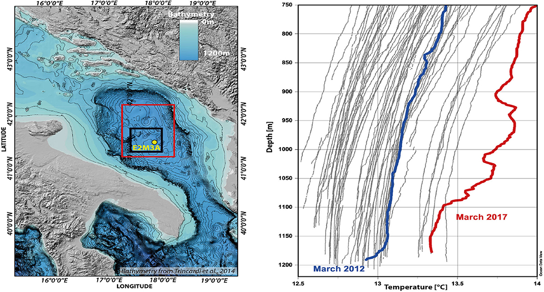
Figure 1. (Left) Region of the South Adriatic Pit (SAP). The red rectangle shows the area where all the profiles originated. After 2010, data were collected within the black rectangle. The yellow dot indicates the position of the E2M3A observatory of the thermohaline time series. (Right) All 55 profiles of the temperature dependence with the depth. The two profiles during the deep convection/gravity current events are emphasized in blue and red.

More specifically, we consider the temperature structure in the area of the dSAP based on a considerable number of observations, starting from 1985 and increasing in number over the last two decades. The dSAP has a maximal depth of approximately 1,230 m and is delimited at the south by the Otranto Sill (780 m deep)(see Figure 1). We focus on the temperature structure below the sill depth. It is significantly different from an exponential structure, as is shown below, and the theory put forward by Munk (1966) has to be supplemented. The Adriatic is also interesting because the tidal motion is negligible (see, e.g., Cushman-Roisin et al., 2001 and references therein), which simplifies the internal dynamics. An advantage of considering the dSAP is that it is easily accessible (only approximately 60 nautical miles from the coast) and has been extensively observed with considerable data coverage in space and time over the last 40 years. The present work relies on two types of data: first, in-situ ship-borne data measurements, 55 vertical temperature and salinity profiles at a 1 m resolution, collected in the dSAP from 1985 to 2019 (Cardin et al., 2011) and second, time series of high-frequency point measurements from 2006 to 2019 at 750, 900, 1,000, and 1,200 m nominal depths from the mooring at the E2M3A Observatory, (http://nettuno.ogs.trieste.it/e2-m3a/). The latter are positioned in the dSAP and are particularly dedicated to the study of the long-term thermohaline and biogeochemical properties. In the present work, the diffusivity processes in the deep layer are analyzed, and thus, only measurements at 750 m (considered as the reference level for the Otranto sill depth) and deeper are taken into consideration.

It was shown by Querin et al. (2016) that the dynamics in the dSAP are forced by intermittent gravity current and deep convection events that reach below the sill depth every few years and that only last from a week to a few months. The most recent events of this type occurred in March and April of 2012 and in March 2017. The former event is due to cold and very dense water from the northern Adriatic (Bensi et al., 2013), whereas the latter event is due to salty and warm water and has, so far, not been discussed in a scientific publication. The subject of the present work is to determine what happens between such events, when the vertical temperature structure is governed mainly by continuous vertical turbulent diffusion as shown by Querin et al. (2016). The different time scales associated with short-lasting convection/gravity current events and continuous diffusion allow separately consideration of the two regimes. In the present work, we investigate continuous mixing based on observational data using the dynamics of the heat equation. The aim is to show that in between deep convection/gravity current events, the dynamics are governed by turbulent diffusion and that a bulk mixing coefficient can be determined to allow efficient parameterization.

The theory is presented in the next section, followed by the description of the experimental data and methodology in section 3. The results for the profiles are given in section 4.3, and those for the time series are given in section 4.4. The results are discussed in section 5, and conclusions are given in section 6.

2. Theory

We consider the vertical temperature structure of the dSAP and ignore the horizontal variations. This is justified by the dominance of horizontal (isopycnal) mixing over vertical (diapycnal) mixing (Ledwell et al., 1998). Conceptually, the Munk solution is not valid in the dSAP, as there is no continuous injection in the deep waters, which justifies a continuous upward velocity. Furthermore, Figure 1 shows that the vertical gradient of the temperature vanishes toward the bottom, which indicates intense mixing without restratification effects. The data from a depth of 750 m down to the bottom have a clearly non-exponential functional form, indicating that the Munk theory of a balance between the upward advection and downward diffusion of heat does not apply. Without upward advection, only vertical turbulent diffusion remains, with no process to balance it and the only stationary solution is a constant temperature in space and time. This is not observed. Instead, the density structure is evolving in space and time with dynamics described by the heat equation, as is demonstrated below.

2.1. Heat Equation

We are interested in the evolution of the temperature T(z, t) in the dSAP deeper than the sill depth (≈ 780 m). The underlying assumption of the present work is, that the dynamics in the dSAP are governed by the forced heat equation:

$\begin{array}{ll}{\partial }_{t}T(z,t)=\kappa {\partial }_{zz}T(z,t)+I(z,t),& (1)\end{array}$

where the only free parameter in the system is the vertical eddy diffusivity κ. The last term represents the intermittent intrusions in the form of deep convection or gravity-current events and is supposed to vanish over extended periods in time. The dynamics evolve between z_s = −750 m, the measurement point closest to the sill depth, and the bottom, z_b = −1, 220 m. The boundary conditions are T(z, t) = T_obs(z_s, t) at the sill depth and ∂_zT(z_b, t) = 0 at the bottom. This shows that the model is forced continuously by a time-dependent heat flux at its upper boundary that deeply diffuses, whereas there is no heat flux at the bottom. This model is called the diffusion-intrusion model in the sequel. It is linear and therefore allows us to separately obtain analytical solutions for different types of forcing and then add them to obtain the overall solution.

The unforced heat equation, Equation (1), is given by I(z, t) = 0 and T_obs(z_s, t)= const. In the long term, the temperature relaxes to the imposed temperature at the sill depth down to the bottom, the only time independent solution. The time-dependent evolution is given by $T^h(z,t)=T_{\text{obs}}(z_s)+r(t)m(z)$, where r(t) and m(z) are related by:

$\begin{array}{ll}\frac{{\partial }_{t}r}{r}=\kappa \frac{{\partial }_{zz}m}{m}=\lambda & (2)\end{array}$

and λ does not depend on z or t, as m is not dependent on t and r is not dependent on z (Please see Zachmanoglou and Thoe, 1986 chapter 9.2 for more details on the calculations and the solution using the “separation of variables”). We further define the following: $\Delta T^h(z,t)=T^h(z,t)-T_{\text{obs}}(z_s,t)$. The boundary conditions of ΔT^h(z, t) = 0 at the upper boundary and a vanishing temperature gradient at the lower boundary lead to the solution of the unforced heat equation of the form (z is given in meters):

$\begin{array}{ll}\Delta T^h(z,t)={\displaystyle \sum _k}{A}_{k}sin(\frac{\pi (2k-1)(z-z_s)}{2(z_s-z_b)})exp(-\mu {(2k-1)}^{2}t).& (3)\end{array}$

Note that only the wave numbers, with odd integers 2k − 1, satisfy the bottom boundary-condition and Equation (2) imposes

$\begin{array}{ll}\mu =\kappa {\left(\frac{\pi }{2(z_s-z_b)}\right)}^2.& (4)\end{array}$

The characteristic e-folding decay time scale for a vertical eddy diffusivity of κ = 5 · 10⁻⁴m²s⁻¹ (see section 4) and for the first mode, k = 1, is μ⁻¹ = κ⁻¹(π/2)⁻²(470m)² ≈ 5.7 years. For the following modes satisfying the boundary conditions, k = 2, 3 the time scales are 9 and 25 times shorter, respectively; the modes are damped in less than a year. The higher order modes (k > 3) are damped within less than a month. The interannual dynamics are therefore dominated by the mode k = 1 (see section 4). This shows that the unforced dynamics consists of a sum of non-interacting sine modes that decay exponentially in time at a rate that is proportional to the square of their wavenumber.

When a time-dependent forcing is applied, the dynamics of each mode are still independent. The coefficients are no longer constant in time, and we define $B_k(t)=A_k(t)exp(-\mu {(2k-1)}^{2}t)$. The first coefficient B₁(t) is obtained by projection on the first mode:

$\begin{array}{ll}{B}_1(t)=\frac{4}{\pi (z_s-z_b)}{\displaystyle {\int }_{z_b}^{z_s}}\Delta T(z,t)sin(\frac{\pi (z-z_s)}{2(z_s-z_b)})dz& (5)\end{array}$

The projection of the data for modes k = 2 and 3 and for data records that do not go to the total depth of 1220 m is given in Appendix 1. The temporal evolution of the coefficients B_k is governed by the initial conditions at t = 0, the heat flux at the sill depth and the intermittent forcing.

In the case of the intermittently forced heat equation, through deep convection or gravity currents, the temperature structure changes, and higher order modes may also have large amplitudes. This intermittent forcing is represented in Equation (1) through the term I(z, t). After a short (several months) intermittent event, the dynamics evolve unforced, and the amplitude of the higher modes decreases rapidly, as explained above. Only a few months after the intermittent forcing, the dynamics are again dominated by the lower order modes.

When the continuously forced heat equation is driven by increasing temperature at a depth of 750 m at a constant rate γ = ∂_tT_obs(−750m, t), the solution is:

$\begin{array}{ll}{T}^{cf}(z,t)=\gamma t+\frac{\gamma }{2\kappa }{(z-z_b)}^2,& (6)\end{array}$

which can be determined by introducing the above equation in Equation (1) with a vanishing inhomogeneous term, I(z, t) = 0. This corresponds to the constant temperature increase of a parabolic shaped temperature profile. The temperature difference between the sill depth and the bottom of the dSAP is constant in time and is related to the temperature increase at the sill depth by:

$\begin{array}{ll}{T}^{cf}(z_s,t)-T^{cf}(z_b,t)=\frac{\gamma }{2\kappa }{(z_s-z_b)}^2& (7)\end{array}$

It is important to note that the quadratic shape is not very different from the first sine mode (see Figure 2), and when it is projected on the sine modes, the amplitudes decay quickly with the wavenumber as (2k − 1)⁻³. The first sine mode explains more than 92.7% of the total variance; for the first three modes, it is almost 97%. This means that from the shape of a single temperature profile at a given time t₀, we cannot significantly determine whether the dynamics are freely decaying or forced by a constant-in-time vertical temperature flux. In other words, $T^{cf}(z,t_0)$ resembles $T^h(z,t_0)$ at a time t₀; however, the evolution in time for the unforced and continuously forced cases is different. In the former case, the amplitude decays exponentially, while in the latter, it stays constant.

FIGURE 2

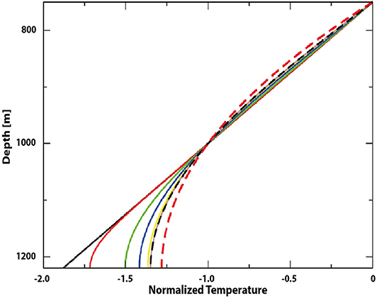
Figure 2. Temperature profiles from the numerical model given by the unforced heat equation (1) (all values are divided by the temperature difference between 750 and 1,000 m depths) for the initial condition (black line), after 1 month (red), 6 months (green), 1 year (blue), 2 years (yellow), and 10 years (brown) of the integration time (κ = 5 · 10⁻⁴m²s⁻¹). The black dashed line is the analytic solution of the first mode, to which the dynamics converge. The red dashed line is the parabolic profile of the continuous forcing.

2.2. Heat Content and Heat Flux

When a linear equation of state is supposed, the heat content, its evolution, the potential energy and its evolution as well as the increase in potential energy by mixing can be obtained independently for every mode k and are determined by the coefficients B_k. If the vertical temperature profile is close to the first sine mode, the heat flux per unit area at the sill depth is

$\begin{array}{ll}H=c_p\kappa \rho {\partial }_{z}T(z_s)=c_p\kappa \rho \frac{\pi (T(z_s)-T(z_b))}{2(z_s-z_b)}& (8)\end{array}$

and the heat content per unit area is:

$\begin{array}{ll}{H}=c_p\rho \frac{2(z_s-z_b)}{\pi }(T(z_s)-T(z_b)).& (9)\end{array}$

The ratio of the heat content and the heat flux is the characteristic time scale of the first mode, which is given in Equation (4).

3. Experimental Data and Methods

In order to validate Munk's theory using experimental data we have considered the area of the South Adriatic (see Figure 1) where mixing and winter convection play an important role in homogenizing the physical and chemical properties of seawater and spreading heat along the water column. To analyze the importance of these processes, two different data sets are used: The first one consists of temperature profiles, taken during ship cruises, covering a long period of time and a large spatial area, and the second is times-series data, with high frequency point measurements along the water column by the E2M3A Observatory. The latter is located in the dSAP and is particularly dedicated to the study of long-term thermohaline and biogeochemical properties. In this study, we analyze the diffusivity processes in the deep layer; therefore, we consider only measurements deeper than 750 m.

3.1. Profiles

The long-term variability of the thermal characteristics of the deep layer in the South Adriatic area is determined based on temperature data collected during several oceanographic campaigns between 1985 and 2019. The cruises were undertaken as part of Italian and European projects, and other datasets were kindly provided by the NATO UNDERSEA RESEARCH CENTER, PANGEA Data Repository (https://www.pangaea.de/) and MEDATALAS Dataset (https://nodc.inogs.it/nodc/). All the profiles were processed following the methodology described by Cardin et al. (2011) and applied for the data between 1990 and 2010, i.e., the oceanographic condition during a specific campaign is represented by a profile obtained by averaging all the CTD casts deeper than 1,000 m measured in the area between 41.25° and 42.25° N and 17.25° and 18.25° E in the SAP (Figure 1). For the studied period, we consider data from 55 temperature profiles deeper than 750 m. The potential temperature (hereafter referred to as temperature) is calculated from the original profiles with the surface as the reference depth. Profiles after 2010 were collected in a narrower area of 0.5^o × 0.5° degrees Lat/Lon located in the dSAP and near the E2M3A Observatory (black square in Figure 1). Further information about these cruise operations, materials and methods can be found at http://www.ogs.trieste.it:8585/biblioteca/.

3.2. Time Series

The data collected at the E2M3A Observatory enables the monitoring of changes that can be linked to variations in the general circulation of the Eastern Mediterranean Sea or, on a larger time scale, to the climate variability in the area, demonstrating the importance of high-frequency measurements to resolving events and rapid processes.

The Observatory has been working almost continuously since the end of 2006, and therefore, the high- frequency time series of physical and biochemical parameters measured at the site can be considered the longest almost continuous offshore data set available in the region (http://nettuno.ogs.trieste.it/e2-m3a/). The temperature was measured using CT-CTD sensors of the SBE37 at a sampled rate of 1 h and SBE16 with a sampling interval of 3 h. For homogeneity, all the time series were averaged on a daily basis, and the temperature values were converted to the potential temperature. A low-pass filter PL33 with a cutoff period of 33 h (Flagg et al., 1976) was applied to remove inertial oscillations (inertial period of 17.593 h at 42° N in the South Adriatic Pit) so that tidal and higher frequency fluctuations do not mask the low-frequency fluctuations in the time series driven by winds and the density field. The filter removes more than 99% of the amplitude at the semidiurnal tidal periods and more than 90% of the amplitude at the diurnal tidal periods. These subinertial non-tidal time series are considered as the starting point for the analysis.

For this study, the time series considered along the mooring line come from 4 instruments positioned at 750, 900, 1,000, and 1,200 m (Cardin and Bensi, 2014; Cardin et al., 2014, 2015, 2018). To simplify the analysis, the depths of the series are nominal. The available data used are from November 2006 to October 2019, with a gap between September 2010 and May 2011. The time series at 900 m started in November 2013. An exhaustive description of the site, data availability and data analysis can be found in Bensi (2012) and Bensi et al. (2014) and at the Observatory webpage (http://nettuno.ogs.trieste.it/e2-m3a/).

All instruments were calibrated and controlled for quality before and after each recovery and deployment, following the procedures indicated in Coppola et al. (2016) and Pearlman et al. (2019). In addition, during recovery or deployment operations, a CTD cast was performed to assess the accuracy of the measured data and to identify possible instrument drift.

3.3. Empirical Orthogonal Function Analysis

To assess the temporal variability and the vertical structure of the water column in the dSAP, we applied empirical orthogonal function analysis (EOF) (Preisendorfer and Mobley, 1988) to the temperature time series. For this purpose, time series at 750, 900, 1,000, and 1,200 m were analyzed.

Unfortunately, the time series shows gaps (not simultaneous) at different levels due to instrument failures, especially in the deepest part of the mooring line in the period from 2006 to 2010 and from 2011 to 2014. Since the EOF analysis requires data at all levels for its application, the data collected before 2014 can not be used for this analysis. Thus, we considered only the time series from September 2014 to August 2019, as it was the longest period without important gaps (only short ones -no longer than 5 days -due to the Observatory service). To eliminate these gaps, the daily time series were subsequently averaged on a weekly time scale. The filtered time series allowed us to study the time scales of interest (e.g., seasonal and interannual).

4. Results

4.1. Numerical Integration

We performed a numerical integration of the heat equation with an imposed temperature at approximately the sill depth T_obs(−750m, t) (Dirichlet boundary condition) and a vanishing gradient at the bottom (1,220 m) (Neumann boundary condition). For illustration, an unforced integration that starts from a linear stratification is represented in Figure 2. All values are divided by the temperature difference between 750 and 1,000 m depths to emphasize the evolution of the shape and the convergence to the first mode. Snapshots are shown at 1 and 6 months and at 1, 2, and 3 years (κ = 5 · 10⁻⁴m²s⁻¹). The convergence to the first sine-mode, shown in Figure 2, with a characteristic time scale of several months, is clearly visible. In the same figure the shape of the parabolic profile for the constant forcing case is also given for comparison.

In the numerical integration, the two types of forcing, with time-dependent temperature variation at the sill depth γ and time and space dependent intermittent forcing I(z, t), can be easily combined. To reproduce the space-time dynamics of the observed data, both types of forcing are applied, and Equation (1) is integrated numerically.

4.2. Eddy Diffusivity

The only free parameter in the heat equation is the diffusivity. The vertical exchange of heat is at least two orders of magnitude larger than that predicted by molecular motion only, and most is performed by turbulent fluid motion. Its parameterization is often achieved by assuming a vertical eddy diffusivity. It cannot be calculated from first principles but has to be determined from observations. It can be obtained based on different data analysis methods. The first method is a best fit of the time evolution of a numerical integration described in section 4.1 to the time-series data discussed in section 3.2. More precisely, we numerically solve Equation (1), which is forced at the upper boundary by imposing the temperature observed at 750 m depth and supplemented by two intermittent injections in 2012 and 2017, modeling the deep convection/gravity current events that penetrate the dSAP. The value of the diffusion constant κ is then estimated so that the evolution of the model best fits the time-series data. The second method is based on Prandtl's mixing-length concept (see Taylor, 1922, 1959; Prandtl, 1925; Bradshaw, 1974). We first calculate a typical r.m.s. vertical scale $\Delta z_{rms}=\sqrt{{(T^{\prime })}^2}/{\partial }_z\overline{T}$ based on the temperature fluctuations T′ at 900 m depth and an average temperature gradient ${\partial }_z\overline{T}$ at the same depth. We also determine the correlation time of the vertical motion by looking at the autocorrelation function of the temperature fluctuations $C(\tau )={\langle T^{\prime }(t+\tau )T^{\prime }(t)\rangle }_t/{\langle {(T^{\prime }(t))}^2\rangle }_t$, which is independent of time t for statistically stationary dynamics. We then obtain the correlation time: ${\tau }_{corr}={\int }_0^{{\tau }_0}C(\tau )d\tau$, where τ₀ is the first zero crossing of C(τ). The vertical eddy diffusivity can then be estimated by:

$\begin{array}{ll}{\kappa }_{\text{turb}}=C_s\frac{{(\Delta z_{\text{rms}})}^2}{{\tau }_{corr}},& (10)\end{array}$

where C_s is a non-dimensional constant. The third method is based on the continuously forced dynamics, which leads to a balance between the temperature increase and the temperature difference between the sill depth and the bottom, as expressed by Equation (7). The three approaches for estimating the vertical eddy diffusivity are performed in sections 4.4 and 4.5.

4.3. Profiles

When considering the 55 temperature profiles taken during the period from 1985 to 2019, which are presented in Figure 1, a similarity of most of them to the first sinusoidal mode depicted in Figure 2 is discernible. For a quantitative analysis, we calculated the coefficients B_k for k = 1, 2, and 3, which are given in Figure 3. Only the amplitude of the first mode has a value which is significantly different from zero, varying around 0.5^o K, while the amplitudes of the second and third mode are typically more than an order of magnitude smaller and have no definite sign. We further calculated the remaining variance not explained by the first mode or the first three modes in Figure 3. For over 2/3 of the profiles, more than 99.5% of the variance can be explained by the first mode and more than 99.85% by the first three modes. Note that the 2017 event is clearly depicted by the atypical profile from 22/03/2017, given in red in Figure 1. The event also has a clear signature in the amplitude of the second and third modes (Figure 3) and in a strong increase in the variability neither explained by the first mode nor by the first three modes (Figure 3). This means that for this profile, higher order modes have an increased amplitude. In the subsequent profile only 4 months later (27/07/2017), the amplitude of the second and third mode as well as the unexplained variability has decreased to the values prior to the event. This is coherent with the fact that the decay times of modes two and three are only a few months, as explained in section 2.1. The decay of even higher modes happens at scales shorter than a month. The 2012 event, however, has no conspicuous signature in the amplitude or variability data. The profile from 31/03/2012 (given in blue in Figure 1) shows that the dense gravity current water is just starting to arrive, and it is seen at the very bottom of the data but does not significantly impact the overall shape of the profile. No profile is available for the rest of the year, and the next profile is 1 year later (23/03/2013); at this time, the second, third and higher modes have faded away.

FIGURE 3

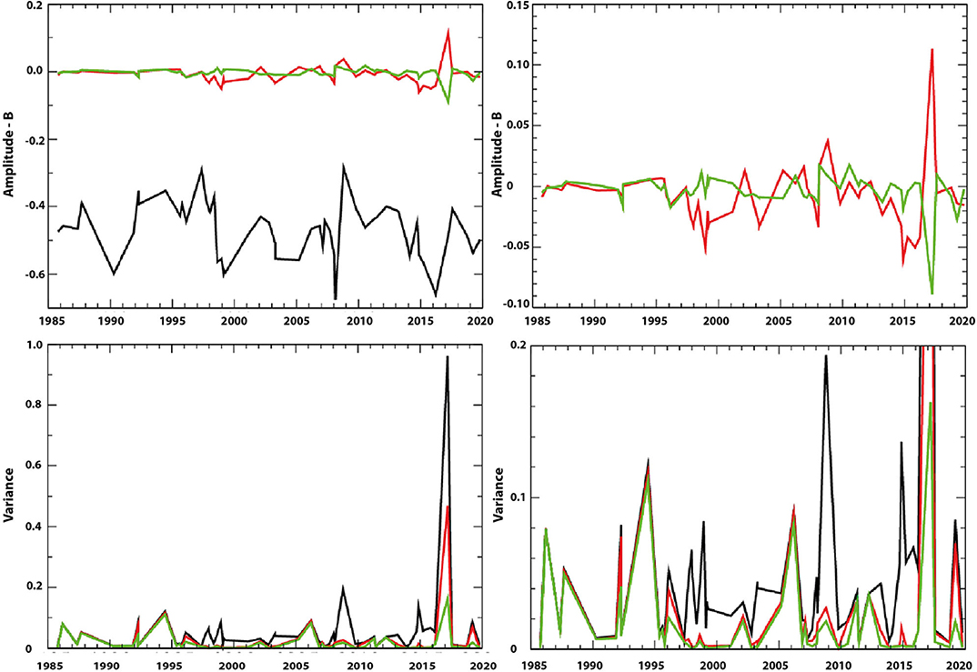
Figure 3. (Upper) Evolution of the amplitudes of the sine modes B₁ (black), B₂ (red), and B₃ (green). The vertical scale gives the temperature difference between the 750 m time series and the maximum profile depth (1,219 m) of the corresponding mode. (Lower) Part of variability not explained by B₁ (black), B₁ + B₂ (red) or B₁ + B₂ + B₃ (green) (left) and zoom (right). Figures on the right show the same data magnified.

4.4. Time Series

We first numerically integrate the diffusion-intrusion model. An integration with ${\kappa }_{\text{fit}}=5·10^{-4}$m²s⁻¹ and two convection or gravity-current events in March 2012 centered at the bottom and in March 2017 centered at z = 1, 100 m manages to reproduce, to a reasonable degree, the observed temperature and salinity evolution, as shown in Figure 4.

FIGURE 4

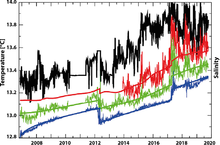
Figure 4. The observational data (thin lines) and the corresponding solutions of the injection-diffusion model (thick lines) for different depths (black 750 m, red 900 m, green 1,000 m, blue 1,200 m) for temperature.

Furthermore, the data at 750 and 1,200 m allows determining the amplitude of the first mode. Using this information and supposing that the higher-order modes are of low amplitude, allows to interpolate for the depths in-between. The obtained values were compared to the observed data at 900 and 1,000 m. Again, we remark a good correspondence between the observational data and the interpolation in Figure 5. A slight deviation is observed between years 2014 and 2017.

FIGURE 5

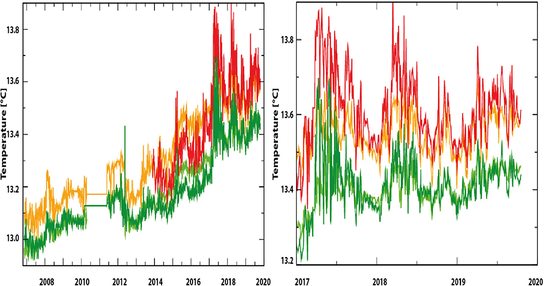
Figure 5. Observed data at 900 m (red) and 1,000 m (light green) and their interpolations 900 m (orange) and 1,000 m (dark green). The right figure is a magnification of the data starting in 2017.

The eddy diffusion can be estimated based on the correlation time and the vertical r.m.s displacement of a fluid parcel, as explained in section 4.2. The former is given by the integral of the correlation function from zero to the first zero crossing. The first zero crossing is at 4 days, and the integral gives τ_corr = 1.6 days (not shown). The latter is calculated based on the temperature fluctuations and the mean temperature gradient (box-averaged over 30 days); its average value lies around Δz_rms = 20 m. When we impose κ_turb = κ_fit we find, using Equation (10), that C_s ≈ 0.18. There is no surprise that it is smaller than one, as some of the vertical motion is due to internal waves, which do not lead to mixing if they do not break. Interestingly, the former is obtained based on turbulent fluctuations on a time scale of a few days, while the latter is obtained based on the evolution of the temperature profile over several years.

4.5. EOF Analysis

The modes of the EOF analysis of the time series and the temporal evolution of EOF mode 1 are presented in Figure 6. Note that the time average is given by EOF mode 0 and that its profile resembles the parabolic profile put forward in section 2.1 for the case with a constant forcing. The dominant evolution is given by EOF mode 1 (describing 87% of the variance), which is close to a constant-in-depth temperature increase. In this case, the temperature increase at the sill depth and the amplitude of mode 0 are related by Equation (7). The amplitude for mode 0 is ΔT = 0.5^o K (see Figure 6A). The warming trend is obtained by taking the product of the vertical average of mode 1 (which is close to constant see Figure 6B) and the trend of its amplitude (see Figure 6C), that is: γ = 0.5 · 0.64^o K/(5years) = 6.4 · 10^−2o K/year. A diffusivity of ${\kappa }_{EOF}=4.5·10^{-4}$ m²s⁻¹ is obtained from Equation (7), which is close to κ_turb and κ_fit. We remind that the Otranto Sill depth is 780 m.

FIGURE 6

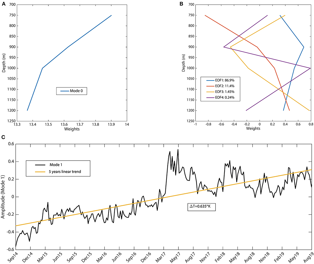
Figure 6. Temporal average of data, EOF mode 0 (A) and the EOF modes 1 to 4 with their variances given in the legend (B). Temporal evolution of the amplitude of EOF mode 1 (C).

The higher order EOF modes 1, 2, and 3 closely resemble discretized versions of the analytic sine modes k = 1, 2, and 3 (wavenumbers 1, 3, and 5). If we suppose that they are subject to random forcing of equal strength and diffusive damping, their relative variance should decrease as 1, 1/9, and 1/25. The observed values are 1, 1/8, and 1/48, which is within discretization and statistical error (the variance of the last EOF mode is only 0.24%).

5. Discussion

All the above results based on temperature measurements show that the action of turbulent mixing in the dSAP can be modeled well by a heat equation with a constant diffusion coefficient in space and time, a prescribed heat flux at the sill depth and a forcing term that represents rare gravity current and deep convection events. The similarity between the empirical EOF analysis results (applied only to a subset of the time series between 2014 and 2019) and a solution of the forced heat equation, with a forcing that imposes a warming trend through a heat flux at 750 m depth, confirms that the heat equation satisfactorily describes the processes in the dSAP.

When the functional form of the first mode for the temperature stratification is assumed to have an amplitude of 0.5^oK, the heat flux of the dSAP is H = 3.3Wm⁻² according to Equation (8), and the heat content is ${H}=6·10^8$Jm⁻² according to Equation (9). These values characterize the heat-budget of the dSAP and can help to validate numerical models and climate dynamics.

The power per square meter necessary to perform turbulent mixing of the mass (based on temperature only) is

$\begin{array}{ll}P=g\alpha \rho {\kappa }_{\text{turb}}\Delta T.& (11)\end{array}$

For a ΔT = 0.5^o K, this parameter is P = 5 · 10⁻⁴W/m². A mixing efficiency of 0.2 leads to a drain of five times more kinetic energy (see, i.e., Osborn, 1980; Peltier and Caulfield, 2003). If the turbulent Prandtl number is unity, we obtain a characteristic vertical shear of ≈ 3 · 10⁻³s⁻¹.

The presented theory and observations show that from 2006 to 2019, the temperature stratification in the dSAP is determined by the continuous warming in the upper part (above the Otranto Sill depth) and the vertical turbulent diffusion. Other processes such as deep convection and gravity currents that penetrate the dSAP are only visible during a few months on two occasions. We obtain an upper (diffusive) limit for the characteristic time scale for the density structure of the dSAP, which is important as it tells us that the long-term changes in the circulation in the area are due to external forcing. The upper 5-year limit is also important for numerical modeling, as it gives a maximum spin-up time for numerical integrations. When the first mode is correctly estimated in the initial conditions of the numerical integration, a spin up of less than a year becomes sufficient, as only modes higher than k = 1 have to spin up.

The main result is that at a high accuracy, the spatio-temporal evolution of the temperature in the dSAP is described by a heat equation based on a constant (in space and time) vertical diffusivity of κ = 5 · 10⁻⁴m²s⁻¹. This value is similar to published values of vertical diffusivities in other regions of the world oceans. Munk (1966), considering several stations in the interior Pacific Ocean over much larger depths, found that the dominant vertical dynamics acting on the temperature were advective diffusive, with κ = 1.3 · 10⁻⁴m²s⁻¹. The eddy diffusivity in deep basins of the North Aegean was estimated to lie between κ = 2 · 10⁻⁴ to 10 · 10⁻⁴m²s⁻¹ below a depth of 500 m (Zervakis et al., 2003). In the deepest part of the Calypso Deep (below 4,400 m), the vertical diffusivity was found to vary around κ = (4 ± 3) · 10⁻³m²s⁻¹ by Kontoyiannis et al. (2016).

6. Conclusions and Perspectives

We showed that the theory proposed by the “Abyssal recipes” of Munk (1966) for the world ocean is valid for the dSAP, a small oceanic basin, when forcing is added. The hypothesis of the present work is that the dynamics in the dSAP are governed by turbulent diffusion and forced by a continuous heat flux at the upper boundary and sporadic deep convection/gravity current events. A hierarchy of models, all based on the heat equation, is used. The simplest are based on the gravest or the three gravest modes of the analytically solved unforced heat equation. It is shown that the heat equation forced by a constant heat flux at the upper boundary has a functional form close to the gravest mode. The most evolved model includes a time-dependent forcing at the upper boundary as well as intermittent convection events that are solved numerically.

The models successfully describe the profiles and their spatio-temporal evolution. The functional form of the profile is described by the gravest mode of the analytical solution of the homogeneous heat equation, while the time series can be fitted well by the numerical solution of the forced heat equation. Two major deep convection/gravity current events are identified in the time series in 2012 and 2017 between 2007 and 2019 (during the winter/spring season). The longest dissipative time scale in the dSAP, associated with the gravest mode, is approximately 5 years. This does not only indicate that within this period, stratification in the dSAP disappears when forcing resides, but it represents an upper bound for the absence of deep convection events penetrating the dSAP. More precisely, when the temperature at the sill depth does not increase and no deep convection event reaches below the Otranto Sill depth within 5 years, the dSAP becomes essentially unstratified, and subsequent convection is likely to reach the bottom of the dSAP. In other words, a constant warming of the water mass above the sill depth prevents deep convection events from reaching the dSAP, and only diffusion remains; however, when there is no warming at the sill depth, a deep convection event will occur at least every 5 years.

The above developed theory about the dynamics of the dSAP allows a simple injection diffusion model of the dSAP to be built. This can be used to study the evolution of the dSAP under climate change scenarios, as well as to parameterize the feedback of the dSAP on the surrounding ocean dynamics. More precisely, the decomposition of modes with different characteristic time scales can be used to parameterize the response of the deep South Adriatic Pit to a specific process. For interannual variability, only the dynamics of the first mode have to be considered, while for a seasonal forcing, only the first two modes have to be taken into account, considerably reducing the complexity of the problem. The next step is to attempt to extrapolate the above findings to the more involved dynamics above the sill depth, where water masses are subject to horizontal advection and air-sea fluxes.

The performance of the theory and data analysis developed in this publication are not limited to the dSAP but can be equally applied to other enclosed pits in the world ocean, away from the direct influence of atmospheric forcing and strong currents. The temperature variation in the dSAP is significantly different from the exponential profile put forward by Munk (1966). As in Munk and Wunsch (1998), we have to ask the question of which process provides the power to perform the mixing in the case of the dSAP, where tides are excluded. This is one of the key open questions in physical oceanography. To answer this question, the synergy of laboratory experiments on the Coriolis platform (Grenoble) of idealized numerical simulations and of fine resolution (in time-and-space) velocity measurements in the dSAP is currently being employed.

The proposed empirical model for the vertical, one-dimensional, structure of the temperature profile, its evolution in time, as well as the determination of the vertical mixing coefficients and the forcing, relies on the synergy between mooring data with dense temporal coverage and a substantial number of profiles, providing fine resolution in the vertical direction. This dataset has been collected during the last four decades, at a single oceanic site and shows the importance of a continuous effort of collecting data over several generations of funding programs.

Data Availability Statement

The original contributions presented in the study are included in the article/supplementary materials, further inquiries can be directed to the corresponding author/s.

Author Contributions

All authors have contributed to the paper. The numerical projection and integration was performed by AW.

Funding

This work was funded by Labex OASUG@2020 (Investissement d'avenir - ANR10 LABX56) and OGS internal funding.

Conflict of Interest

The authors declare that the research was conducted in the absence of any commercial or financial relationships that could be construed as a potential conflict of interest.

Acknowledgments

Part of this work was performed when AW visited OGS and VC visited LEGI. We thank the OGS ExO and TECDEV Group so as the Captain and crew of the RV OGS Explora and RV Laura Bassi for the valuable support and work during the maintenance of the E2M3A Observatory.

References

Bensi, M. (2012). Thermohaline variability and mesoscale dynamics observed at the E2M3A deep-site in the South Adriatic Sea (Ph.D. thesis). Universita degli studi di Trieste, Trieste, Italy. Available online at: https://www.openstarts.units.it/handle/10077/7387

Google Scholar

Bensi, M., Cardin, V., and Rubino, A. (2014). “Thermohaline variability and mesoscale dynamics observed at the deep-ocean observatory e2m3a in the southern Adriatic sea,” in The Mediterranean Sea: Temporal Variability and Spatial Patterns, Geophysical Monograph Series, eds G. L. E. Borzelli, M. Gačić, P. Lionello, and P. Malanotte-Rizzoli (Oxford, UK: John Wiley & Sons, Inc.), 139–155.

Google Scholar

Bensi, M., Cardin, V., Rubino, A., Notarstefano, G., and Poulain, P. (2013). Effects of winter convection on the deep layer of the southern adriatic sea in 2012. J. Geophys. Res. Oceans 118, 6064–6075. doi: 10.1002/2013JC009432

CrossRef Full Text | Google Scholar

Bradshaw, P. (1974). Possible origin of prandt's mixing-length theory. Nature 249, 135–136.

Google Scholar

Cardin, V., and Bensi, M. (2014). E2m3a-2006-2010-Time-Series-Southadriatic. doi: 10.6092/36728450-4296-4E6A-967DD5B6DA55F306

CrossRef Full Text | Google Scholar

Cardin, V., Bensi, M., and Pacciaroni, M. (2011). Variability of water mass properties in the last two decades in the south adriatic sea with emphasis on the period 2006–2009. Continent. Shelf Res. 31, 951–965. doi: 10.1016/j.csr.2011.03.002

CrossRef Full Text | Google Scholar

Cardin, V., Bensi, M., Siena, G., and Ursella, L. (2014). E2m3a-2011-2013-Timeseries-Southadriatic. OGS (Istituto Nazionale di Oceanografia e di Geofisica Sperimentale), Division of Oceanography. doi: 10.6092/84CB588D-97E5-4C64-91BBBA6109DFA530

CrossRef Full Text | Google Scholar

Cardin, V., Bensi, M., Ursella, L., and Siena, G. (2015). E2m3a-2013-2015-Time-Series Southadriatic. OGS (Istituto Nazionale di Oceanografia e di Geofisica Sperimentale), Division of Oceanography. doi: 10.6092/F8E6D18E-F877-4AA5-A983-A03B06CCB987

CrossRef Full Text | Google Scholar

Cardin, V., Bensi, M., Ursella, L., and Siena, G. (2018). E2m3a-2015-2017-Timeseries-Southadriatic. OGS (Istituto Nazionale di Oceanografia e di Geofisica Sperimentale), Division of Oceanography. doi: 10.6092/238B5903-A173-4FC3-AC5F-5FEDF1064A39

CrossRef Full Text | Google Scholar

Coppola L, Ntoumas M, Bozzano R, Bensi, M., Hartman, S. E., Charcos, L. M., et al. (2016). Handbook of Best Practices for Open Ocean Fixed Observatories 2016 (European Commission, FixO3 project, FP7 Program 2007-2013 under grant agreement no 312463). JCOMM Technical Reports Community Practices. Available online at: http://hdl.handle.net/11329/302

Google Scholar

Cushman-Roisin, B., Gacic, M., Poulain, P.-M., and Artegiani, A. (2001). Physical Oceanography of the Adriatic Sea: Past, Present and Future. Dordrecht: Springer Science & Business Media.

Google Scholar

de Lavergne, C., Falahat, S., Madec, G., Roquet, F., Nycander, J., and Vic, C. (2019). Toward global maps of internal tide energy sinks. Ocean Modell. 137, 52–75. doi: 10.1016/j.ocemod.2019.03.010

CrossRef Full Text | Google Scholar

Flagg, C., Vermersch, J., and Beardsley, R. (1976). Report on the 1974 MIT New England Shelf Dynamics Experiment, Part 2; the moored Array. Department of Meteorology, Massachusetts Institute of Technology. Lab. Rep. (Unpublished.).

Google Scholar

Kontoyiannis, H., Lykousis, V., Papadopoulos, V., Stavrakakis, S., Anassontzis, E., Belias, A., et al. (2016). Hydrography, circulation, and mixing at the calypso deep (the deepest Mediterranean trough) during 2006–09. J. Phys. Oceanogr. 46, 1255–1276. doi: 10.1175/JPO-D-15-0198

CrossRef Full Text | Google Scholar

Landsberg, H. E., and Van Mieghem, J. (eds.). (1959). Proceedings of Symposium on Atmospheric Diffusion and Air Pollution, Vol. 6. New York, NY; London: Elsevier; Academic Press, 101–112.

Google Scholar

Ledwell, J. R., Watson, A. J., and Law, C. S. (1998). Mixing of a tracer in the pycnocline. J. Geophys. Res. Oceans 103, 21499–21529.

Google Scholar

Munk, W., and Wunsch, C. (1998). Abyssal recipes II: energetics of tidal and wind mixing. Deep Sea Res. I Oceanogr. Res. Pap. 45, 1977–2010. doi: 10.1016/S0967-0637(98)00070-3

CrossRef Full Text | Google Scholar

Munk, W. H. (1966). “Abyssal recipes,” in Deep Sea Research and Oceanographic Abstracts (Citeseer), 707–730.

Google Scholar

Osborn, T. (1980). Estimates of the local rate of vertical diffusion from dissipation measurements. J. Phys. Oceanogr. 10, 83–89. doi: 10.1175/1520-0485(1980)010<0083:EOTLRO>2.0.CO;2

CrossRef Full Text | Google Scholar

Pearlman, J. S., Bushnell, M., Coppola, L., Buttigieg, P. L., Pearlman, F., Simpson, P., et al. (2019). Evolving and sustaining ocean best practices and standards for the next decade. Front. Mar. Sci. 6:277. doi: 10.3389/fmars.2019.00277

CrossRef Full Text | Google Scholar

Peltier, W., and Caulfield, C. (2003). Mixing efficiency in stratified shear flows. Annu. Rev. Fluid Mech. 35, 135–167. doi: 10.1146/annurev.fluid.35.101101.161144

CrossRef Full Text | Google Scholar

Prandtl, L. (1925). 7. bericht über untersuchungen zur ausgebildeten turbulenz. Zeitschrift für Angewandte Mathematik und Mechanik 5, 136–139.

Google Scholar

Preisendorfer, R. W., and Mobley, C. D. (1988). Principal component analysis in meteorology and oceanography. Dev. Atmos. Sci. 17:425.

Google Scholar

Querin, S., Bensi, M., Cardin, V., Solidoro, C., Bacer, S., Mariotti, L., et al. (2016). Saw-tooth modulation of the deep-water thermohaline properties in the southern Adriatic sea. J. Geophys. Res. Oceans 121, 4585–4600. doi: 10.1002/2015JC011522

CrossRef Full Text | Google Scholar

Taylor, G. I. (1922). Diffusion by continuous movements. Proc. Lond. Math. Soc. 2, 196–212.

Google Scholar

Vallis, G. K. (2017). Atmospheric and Oceanic Fluid Dynamics. Cambridge, MA: Cambridge University Press.

PubMed Abstract | Google Scholar

Vic, C., Garabato, A. C. N., Green, J. M., Waterhouse, A. F., Zhao, Z., Melet, A., et al. (2019). Deep-ocean mixing driven by small-scale internal tides. Nat. Commun. 10, 1–9. doi: 10.1038/s41467-019-10149-5

PubMed Abstract | CrossRef Full Text | Google Scholar

Zachmanoglou, E. C., and Thoe, D. W. (1986). Introduction to Partial Differential Equations With Applications. Baltimore, MD: Courier Corporation.

Google Scholar

Zervakis, V., Krasakopoulou, E., Georgopoulos, D., and Souvermezoglou, E. (2003). Vertical diffusion and oxygen consumption during stagnation periods in the deep north Aegean. Deep Sea Res. I Oceanogr. Res. Pap. 50, 53–71. doi: 10.1016/S0967-0637(02)00144-9

CrossRef Full Text | Google Scholar

Zore-Armanda, M., Bone, M., Dadic, V., Morovic, M., Ratkovic, D., Stojanoski, L., et al. (1991). Hydrographic properties of the adriatic sea in the period from 1971 through 1983. Acta Adriatica 32:5544.

Google Scholar

A. Projection

The discretized version of the projection to obtain the amplitude of the modes is given for the first three modes, it is defined iteratively by:

$\begin{array}{l}{B}_1(t)=\frac{{\lambda }_1}{2·469}{\displaystyle \sum _{i=750}^{1219}}\Delta T(i,t)sin(\frac{\pi (i-z_s)}{2·469m})\\ B_2(t)=\frac{{\lambda }_2}{2·469}{\displaystyle \sum _{i=750}^{1219}}\left(\Delta T(i,t)-B_1(t)sin(\frac{\pi (i-z_s)}{2·469m})\right)& (\mathrm{A1})\end{array}$

$\begin{array}{ll}sin(3\frac{\pi (i-750m)}{2·469m})& (\mathrm{A2})\end{array}$

$\begin{array}{l}{B}_3(t)=\frac{{\lambda }_3}{2·469}{\displaystyle \sum _{i=750}^{1219}}(\Delta T(i,t)-B_1(t)sin(\frac{\pi (i-z_s)}{2·469m})\\ -B_2(t)sin(3\frac{\pi (i-750m)}{2·469m}))sin(5\frac{\pi (i-750)}{2·469m})& (\mathrm{A3})\end{array}$

If the record is over the total length λ_k = 1. If the record stops at length $z_B^{\prime }<1,219m$, so does the summation in Equations (A1)–(A3) and:

$\begin{array}{ll}{\lambda }_k={\left(\frac{z_B^{\prime }-z_s}{469m}-\frac{sin(2(k-1)\pi \frac{z_B^{\prime }-z_s}{469m})}{2(k-1)\pi ·469m}\right)}^{-1}& (\mathrm{A4})\end{array}$