A Regional Frequency Analysis of Tide Gauges to Assess Pacific Coast Flood Risk

Introduction

Coastal flood risk is on the rise along many coastlines. Along the densely populated coastlines of the U.S that are well-monitored by tide gauges (TGs), the annual rate of high tide flooding impacting roadways, storm and wastewater systems, and commerce is accelerating and has doubled nationally since 2000 (Sweet and Park, 2014; Sweet et al., 2020). Here, and elsewhere, the primary reason is sea level rise, with >9 cm occurring globally since the early 1990s (Hamlington et al., 2019; Thompson et al., 2019) and even higher rise of relative sea levels (RSL) from regional variability and land subsidence (Kopp et al., 2015).

Across the Pacific Basin and its vast coastlines, decision makers are also facing mounting impacts from rising seas and they need flood risk information to plan and implement well-timed adaptation solutions (Keener et al., 2018). Unfortunately, risk quantification at space scales useful for decision-making is challenging across the Pacific Basin. Extreme events like tropical cyclones are common, extreme climatic variability is constantly occurring [e.g., from the El Nino Southern Oscillation (ENSO)], bathymetries are complex (e.g., islands), and TGs needed to support risk assessments are relatively sparse. With a global sea level rise of 0.5 m (or more) projected by 2100 under a reduced emissions scenario (Church et al., 2013; Oppenheimer et al., 2019) and impacts and expenditures mounting (Moftakhari et al., 2017), the need for contemporary and future projected estimates of coastal flood risk by decision makers here and elsewhere is growing (Le Cozannet et al., 2017; Hall et al., 2019; Kopp et al., 2019).

The basis for assessing contemporary coastal (ocean) flood risk depends upon local extreme sea level (ESL) probabilities from TGs (Figure 1A) to map associated exposure (Kulp and Strauss, 2019) as shown in Figure 1B. Future estimates typically include localized RSL projections (e.g., Hunter, 2012; Tebaldi et al., 2012; Church et al., 2013; Kopp et al., 2014; Sweet and Park, 2014; Buchanan et al., 2017; Wahl et al., 2017; Ghanbari et al., 2019; Oppenheimer et al., 2019; Frederikse et al., 2020; Taherkhani et al., 2020). Most of these studies use the 100-year ESL (1% annual chance level) as a suitable flood threshold to assess impacts and communicate risk, though empirically derived height thresholds for flooding of various severities is preferable as to align with actual infrastructure vulnerabilities and weather warnings affecting daily decision making (Sweet and Park, 2014; Sweet et al., 2018). A drawback is that singular TG records suffer from record-length bias (e.g., short records), and from the perspective of a particular location, under-sample regionally significant rare events like land-falling tropical cyclones leading to large uncertainties in important (e.g., 100-year) ESLs (Hall et al., 2016; Wahl et al., 2017; Figure 1C). Assessments using dynamical models increase spatial coverage and inclusion of synthetic storms are capable of lengthening the record-length of rare event sampling (Lin et al., 2012, 2019; Haigh et al., 2014a,b; Nadal-Caraballo et al., 2015; Vitousek et al., 2017; Vousdoukas et al., 2018; Muis et al., 2020). However, dynamical models usually perform poorly in areas with high TC activity with complex bathymetries (Muis et al., 2016). Recent studies using satellite altimeter (Lobeto et al., 2018) and Bayesian hierarchical models of TG data (Calafat and Marcos, 2020) show promise, but neither have been applied along Pacific Basin coastlines to our knowledge.

FIGURE 1

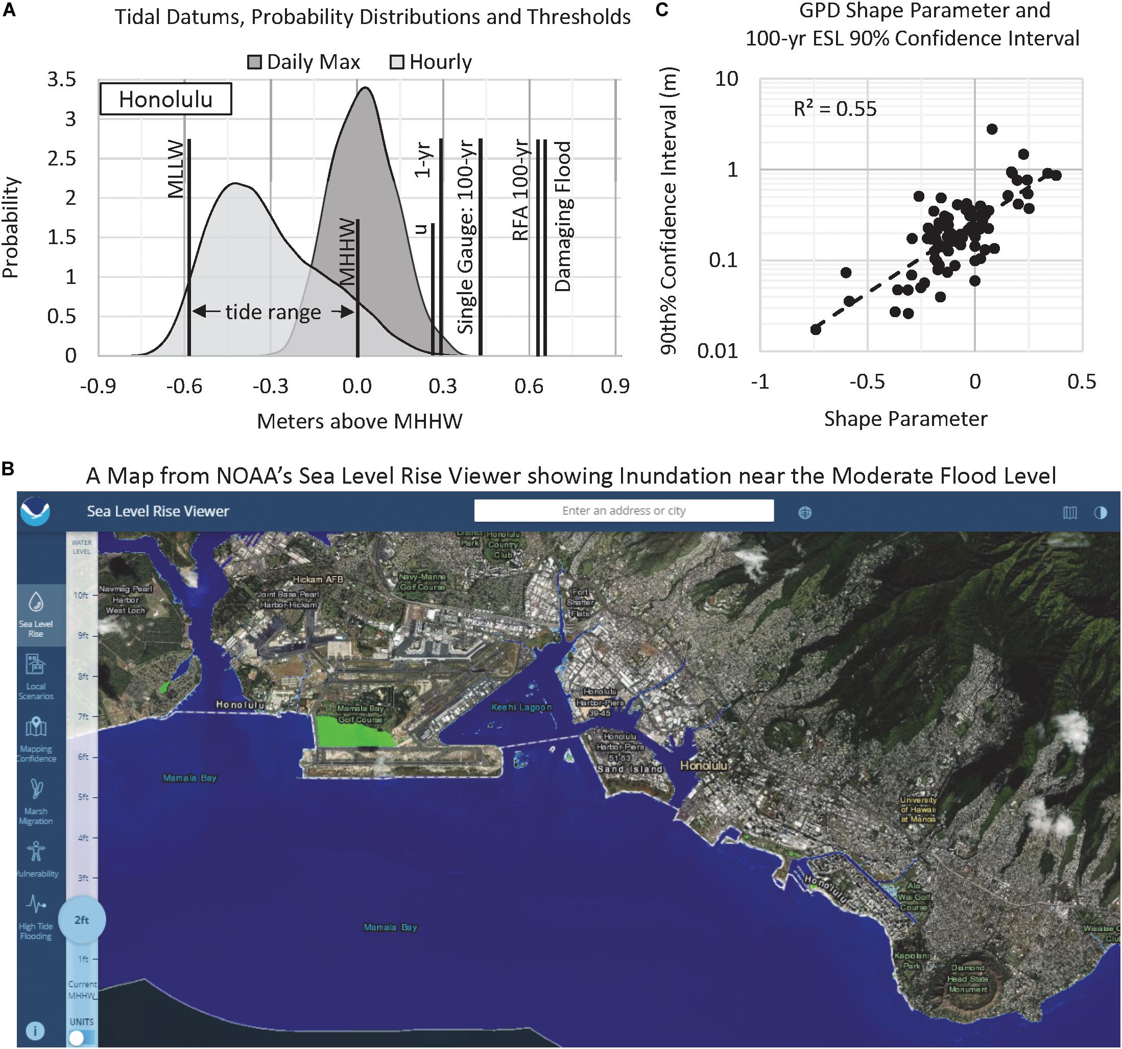
Figure 1. (A) Empirical probability distributions of hourly and daily highest water levels at the NOAA TG in Honolulu with tidal datums [mean lower low water (MLLW), mean higher high water (MHHW) and tide range], the 1- and 100-year extreme sea level probabilities and a proposed Pacific damaging flood threshold for Honolulu. In (B) is a map from NOAA’s Sea Level Rise Viewer for Honolulu (https://coast.noaa.gov/slr/#/layer/slr) showing 0.6 m (2 feet) of inundation that is slightly below the damaging flood level. In (C) is the GPD shape parameter values based upon a single TG analysis from this study and the spread of the 90% confidence interval from all TGs with an exponential fit. Positive shape parameters generally occur where extreme outliers (e.g., tropical storm surges) tend to occur.

In this study, we estimate ESL probabilities and those specifically for damaging flood heights along Pacific coastlines. Our criteria for a damaging flood are calibrated to U.S. National Oceanic and Atmospheric Administration (NOAA) coastal flood thresholds for weather-related hazards along a variety of U.S. Pacific coastlines. We use a regional frequency analysis (RFA) of TG data building upon efforts of Hall et al. (2016), who supported a flood risk assessment of U.S. Department of Defense coastal installations worldwide. In our usage, the RFA method is used to aggregate sets of TG threshold exceedances across particular Pacific basin regions and fit the data with a Generalized Pareto Distribution (GPD) to form a regional ESL probability distribution. A RFA-based assessment provides three key advantages as compared to a single-TG analysis only (Hosking and Wallis, 1997). (1) Rare-event sampling is increased by combining data within a region to provide a more robust parameterization. (2) Shorter TG records are lengthened by regional data to reduce record length bias. (3) Regional ESL probabilities can be downscaled even where there are no TGs if a reasonable localization factor is available.

Our paper has four main components. First, we identify statistically homogeneous regions and for the RFA and fit Pacific TG threshold exceedances with a GPD to estimate regional ESL probabilities (subannual to 500-year). Next, methods to obtain the necessary localization factor to downscale the regional ESL probabilities are presented with results compared to recent sets of foundational results using both TGs and advanced tide and storm surge modeling. Then, we define a Pacific-wide height threshold for a damaging flood. Lastly, we assess the current risk of the damaging flood heights under current sea levels and show how this risk will change under current flood defenses using RSL rise projected by the Intergovernmental Panel of Climate Change (IPCC, Oppenheimer et al., 2019) under Representative Concentration Pathways (RCP) 4.5 (IPCC, 2014).

Materials and Methods

The RFA method (Hosking and Wallis, 1997) is based upon the assumption that regional environments with similar forcing attributes experience a similar event frequency and (extreme) probability density up to a local flood index (u), which is a local scaling factor that captures response peculiarities (Dalrymple, 1960). A RFA uses regional sets of data locally normalized by their respective u with a statistical heterogeneity test (H value) to assess the extent that the data are sufficiently similar. Using statistical L-moments, heterogeneity is a measure of the variation between sites of a location’s summary distribution statistics relative to the amount of dispersion expected if the locations were indeed a homogeneous region (Hosking and Wallis, 1997). If H < 1, the region is considered acceptably homogeneous. If 1 ≤ H < 2, the region is considered possibly heterogeneous, but acceptable for our study. If H ≥2, then the TG group is definitely heterogeneous and not suitable for analysis. Where H ≥2, a discordancy measure that also uses L-moments is used to pinpoint and remove individual locations whose sample L-moment ratios are an outlier within a region (Hosking and Wallis, 1997). Once the regional bounds are established whose data is acceptably homogeneous, the aggregated data is fit with an extreme value distribution. RFA has been useful in river (Michele and Rosso, 2001; Smith et al., 2015), rainfall (Roth et al., 2012; Carreau et al., 2017; Perica et al., 2018), wave height (Weiss et al., 2014), tsunami (Hosking, 2012), and coastal storm surge (Bardet et al., 2011; Bernardara et al., 2011; Weiss and Bernardara, 2013; Frau et al., 2018) studies.

In our study, hourly TG observations with >10 years of record archived by the University of Hawaii Sea Level Center are used and referenced to mean higher high water (MHHW; NOAA, 2003) to help normalize for tide range differences. MHHW is approximated as a 19-year (or record length if < 19 years of data; Supplementary Table 1) average of daily highest water levels. Also used is tide range defined as the difference between MHHW and mean lower low water (MLLW), which is approximated as a 19-year average of daily lowest water levels (NOAA, 2003). Observations from TGs with >20 years of record are linearly detrended and centered with respect to 1992 (i.e., the trend line intercepts the x-axis at the year 1992) similar to methods of NOAA (Zervas, 2013) to align with the midpoint of the current (1983–2001) national tidal datum epoch. Alignment is important as NOAA’s real-time observations and tide predictions along the U.S. West Coast and coastlines of Alaska, Hawaii and the US Pacific Affiliated Islands currently reference the 1983–2001 epoch¹. From the hourly data, daily highest water levels are declustered at each TG using a 4-day storm window to ensure event independence. The 98th percentile of the declustered daily highest levels at each TG is both the threshold to assess exceedances and is also the flood index to localize the RFA ESL probabilities (described below; henceforth, both are referred to as “u” and are the same quantity).

To identify RFA homogeneous regions, we start with the classifications of Rueda et al. (2017) for the Pacific, who divide the global ocean in terms of physical processes (storm surge, tides and wave effects) and their influence inherent within ESL probabilities (Figure 2 and Supplementary Table 1). Within our Pacific study region are Rueda et al. (2017) Tide-dominated (T), Tropical Cyclone (TC), Extratropical (ET), Wave-dominated (W), and Transition (TR) regional classifications. The first step is to regionally aggregate the normalized (by local u value) set of TG threshold exceedances within each of Rueda et al. (2017) classifications. Next, the regional data are spatially declustered with an additional 4-day storm window to ensure that only the maximum water level across TGs within a region is retained (removes any lesser peak water levels from the same event). Then, the statistical heterogeneity measure (H) is estimated and where H ≥2, the TG groups were further subdivided based on the following: sub-classifications from Rueda et al. (2017), geographic divisions (e.g., northern latitude vs. southern latitude stations), and/or the Discordancy measure of a particular TG. In some instances, a TG fit multiple regions and the choice was to keep island groups together as long as the group’s H value was <2 (e.g., Hawaiian Islands).

FIGURE 2

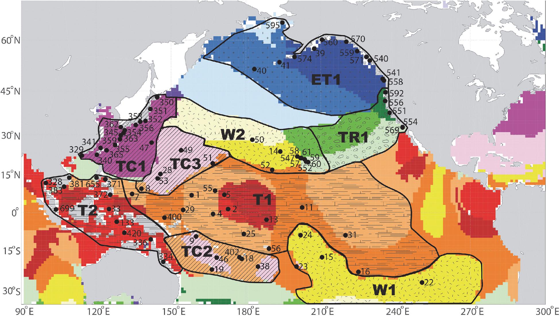
Figure 2. TGs with the University of Hawaii Sea Level Center numbering designation and the RFA homogeneous Tide-dominated (T), Tropical Cyclone (TC), Extratropical (ET), Wave-dominated (W), and Transition (TR) regions delineated in this study based upon the color-shaded classifications of Rueda et al. (2017). The Rueda et al. (2017) shape-file classifications were shared by the authors as licensed under CC BY 4.0.

For example, Rueda et al. (2017) identified two sub-classifications in the Wave region: one that is wave-tide dominant and one that is wave dominant. Within the Pacific, the Wave regions (yellow and whitish-yellow hue colored regions in Figure 2) were located in two areas—one north of the equator and one south of the equator. The main Hawaiian Islands straddle two groups—the wave-tide dominant sub-classification (yellow region in Figure 2) of the Wave region and two sub-classifications (greenish colored regions in Figure 2) within the Transition Region (wave-tide dominant and tide dominant). In order to keep the Island groupings together, we included the main Hawaiian Islands in the Wave Region. We initially grouped TGs from all sub-classifications and the HI stations as one region within the Pacific (13 stations), but the H value was not resolvable. We further separated this group (W1 and W2) based on geographic location (one group north of the equator and one south of the equator). For the southern group (W1), we included Rarotonga, Cook Islands (#23). Technically this station sits in the Tide (T1) region, but it borders the Wave (W1) region and when included within the T1 region its high discordancy resulted in an H value > 2. This region (W1) resulted in an H value of -0.28, which is considered homogeneous. The northern group including the Hawaiian Island stations (W2) resulted in an H value of 1.67, which is considered possibly (acceptably) homogeneous.

With the TG regions established (Figure 2), the aggregated and normalized sets of TG threshold exceedances are fit with a GPD (Coles, 2001) using the penalized maximum likelihood method (Coles and Dixon, 1999; Frau et al., 2018) to estimate (median) regional ESL (RESL) probabilities and the 5th and 95th% levels (90% confidence interval) defined as:

$$\text{G}(\text{Z};\mathrm{u},\mathrm{\alpha },\mathit{\text{ξ}})=\mathrm{\lambda }{\left[1+\xi \left(\frac{\text{z}-\text{u}}{\mathrm{\alpha }}\right)\right]}^{-\frac{1}{\mathit{\text{ξ}}}},(1)$$

where G is the exceedance probability (P[Z > z]), λ is the probability of an individual (normalized) observation exceeding the threshold (u), _α is the scale parameter, and _ξ is the shape parameter. It is assumed that the distribution of the number of exceedances per year follows a Poisson distribution and the return level (e.g., 100-year) for an ESL of height (z) is given by

$${\text{Z}}_{\text{N}}=\mathrm{u}+\frac{\mathrm{\alpha }}{\mathit{\text{ξ}}}\left[{\left({\text{Nn}}_{\text{y}}\mathrm{\lambda }\right)}^{\xi }-1\right],(2)$$

where N is the annual return interval (∼0.3–500-year level), n_y is number days per year (365.25) and _λ is the average number of event exceedances/year (about 3.15 on average across all TGs in the study).

In our RFA approach using GPD, the local ESLs (LESLs) including the model of expected values and their 90% confidence interval at a particular location is given as

$$\mathrm{LESL}={\mathrm{RESL}}^{*}\mathrm{u}+\mathrm{u},(3)$$

where RESL is the regional return level for a particular homogeneous TG region and u is the local flood index. The RESLs are first multiplied by u to localize the values (i.e., LESLs relative to the local u value), which is then added to u to put the LESL results onto MHHW (u is a height above MHHW; Figure 1A). The uncertainty of RESL, as determined from RFA is assumed to be _{σ _RESL}. When localized at any of the TGs used in our study (LESL), u is assumed to have no uncertainty. It is recognized that values of u will have time-dependent characteristics, e.g., similar to those identified in the location parameter of the Generalized Extreme Value (GEV) distribution (e.g., Menéndez and Woodworth, 2010). To our knowledge, no other studies consider or include uncertainties of u within GDP-based estimates of ESL probabilities.

Methods to obtain a prediction or estimate of u and its uncertainty [i.e., root mean squared error (RMSE)] are provided to localize the RESL probabilities and confidence intervals for coastlines (Figure 2) without existing TG data or perhaps a few years of data only. The first method provides a prediction of u and its uncertainty based upon a linear dependence that exists between tide range and u at the Pacific TGs. Tide range information is readily available along most coastlines and islands, e.g., from models calibrated by the global set of TGs and/or satellite altimetry (e.g., https://www.aviso.altimetry.fr/data/products/auxiliary-products/global-tide-fes.html; https://vdatum.noaa.gov/; https://tidesandcurrents.noaa.gov/tide_predictions.html). The other option provides an estimate of the uncertainty in u as a function of a 1–19 record length. For simplicity, an RMSE estimate of u is assessed for the set of Pacific TGs as a whole. To compute the RMSE, we first find the maximum absolute differences between u derived over the entire record (Supplementary Table 1) and for progressively longer consecutive record lengths between 2001 and 2019 at each TG (e.g., 19 discrete 1-year records; 18 overlapping 2-year records, etc.). We use the maximum (absolute) difference at each TG to account for potential interannual variability that can be extreme (e.g., due to phases of ENSO). This difference is considered the error in estimating u for shorter records and the average of the absolute differences across all TGs is considered the bias. The standard deviation of the absolute differences is also computed across all TGs and an estimate of the RMSE is then computed as the square root of the sum of the square of the bias and the standard deviation (variance).

When using predicted values or short-record estimates of u, the uncertainty estimates of LESL will include additional uncertainty in _{u  σ _u}. For simplicity, we assume that RESL (estimated from the regional return level curve) and u are independent and derive an expression for variance of LESL (${\mathrm{\sigma }}_{\text{LESL}}^2)$as follows:

First, using Eq. (3), ${\mathrm{\sigma }}_{\text{LESL}}^2=\text{Var}\left[{\text{RESL}}^{*}\text{u}\right]+\text{Var}\left[\text{u}\right]+2\text{Cov}[{\text{RESL}}^{*}\text{u},\text{u}]$ where Var and Cov represent the variance and the covariance, respectively, of terms inside the square brackets. It may be shown (Mood et al., 1974) that $\text{Var}\left[{\text{RESL}}^{*}\text{u}\right]={\mathrm{\mu }}_{\text{u}}^2{\mathrm{\sigma }}_{\text{RESL}}^2+{\mathrm{\mu }}_{\text{RESL}}^2{\mathrm{\sigma }}_{\text{u}}^2+{\mathrm{\sigma }}_{\text{u}}^2{\mathrm{\sigma }}_{\text{RESL}}^2$ where _μ and _{σ ^2} are the expected value and the variance of the variable indicated in the subscript. Also, the covariance term above simplifies to: $\text{Cov}[{\text{RESL}}^{*}\text{u},\text{u}]={\mathrm{\mu }}_{\text{u}}{\mathrm{\sigma }}_{\text{u}}^2$. Combining the above expressions, we obtain:

$${\mathrm{\sigma }}_{\text{LESL}}^2=\left[{(1+{\mathrm{\mu }}_{\text{RESL}})}^2+{\mathrm{\sigma }}_{\text{RESL}}^2\right]{\mathrm{\sigma }}_{\text{u}}^2+{\mathrm{\mu }}_{\text{u}}^2{\mathrm{\sigma }}_{\text{RESL}}^2(4)$$

where _{μ _RESL} and _{μ _u} are the expected values of the regional return levels and the expected value of u, for example, predicted by the tide-range and u dependency, respectively, and ${\mathrm{\sigma }}_{\text{u}}^2$ is the uncertainty inherent to any u-prediction relationship (e.g., RMSE). It should be noted that the added uncertainty in u as estimated from this relationship would introduce additional uncertainty in estimates of LESL.

Derivation of a threshold defining a damaging flood height builds upon patterns found by Sweet et al. (2018) between discrete coastal flood thresholds of NOAA’s National Weather Service and local tide range. NOAA’s National Weather Service² coastal flood thresholds are empirically calibrated over years of impact monitoring, define infrastructure vulnerabilities and used to warn emergency managers of forecasted impacts. Projections of RSL rise under RCP4.5 used to assess future changes in flood risk come from the IPCC Special Report on the Ocean and Cryosphere in a Changing Climate (SROCC; Oppenheimer et al., 2019). To estimate LESLs with return intervals down to a 0.1-year event frequency, we extrapolate our GPD model with a logarithmic fit for return levels between 2 years and the ∼0.3 years (1/_λ) limit, with results that are in agreement with those of Sweet et al. (2018).

Findings

The RESL probabilities span from about 0.3- to 500-year levels and are shown in Figure 3 (values also listed in Supplementary Table 2) as return level curves following common engineering practice along with the GPD model parameters and their uncertainties. The regional return level curves show where RESL probabilities are limited (bounded) or not (unbounded) as quantified by either a negative or positive shape parameter, respectively. Unbounded regions include TC regions 1 and 3 and W regions 1 and 2. Visual inspection of the regional return level curves show a satisfactory fit to the data, though outliers within the extreme tails are noticeable mainly within regions TC3 and W2 (Figure 3). These outliers (data near/above the 90% confidence interval) suggest a mixed response from tropical and extratropical cyclones (Haigh et al., 2014a), which is reflected in their higher heterogeneity measure (H values in TC3 and W2 of 1.39 and 1.67, respectively in Supplementary Table 2). Indeed, outlier data in region TC3 include several tropical storm surges measured at Saipan (TG #28), Yap (TG #8), and Wake Island (TG #51). Region W2 contains tropical storm surges measured at Johnston Atoll (TG #52) and a record-setting event in response to Hurricane Iniki, which hit Hawaii in 1992 and whose surge (e.g., 0.96 m above MHHW at Kauai–TG #58) produced highest TG-measured water levels ever along the Hawaiian Islands.

FIGURE 3

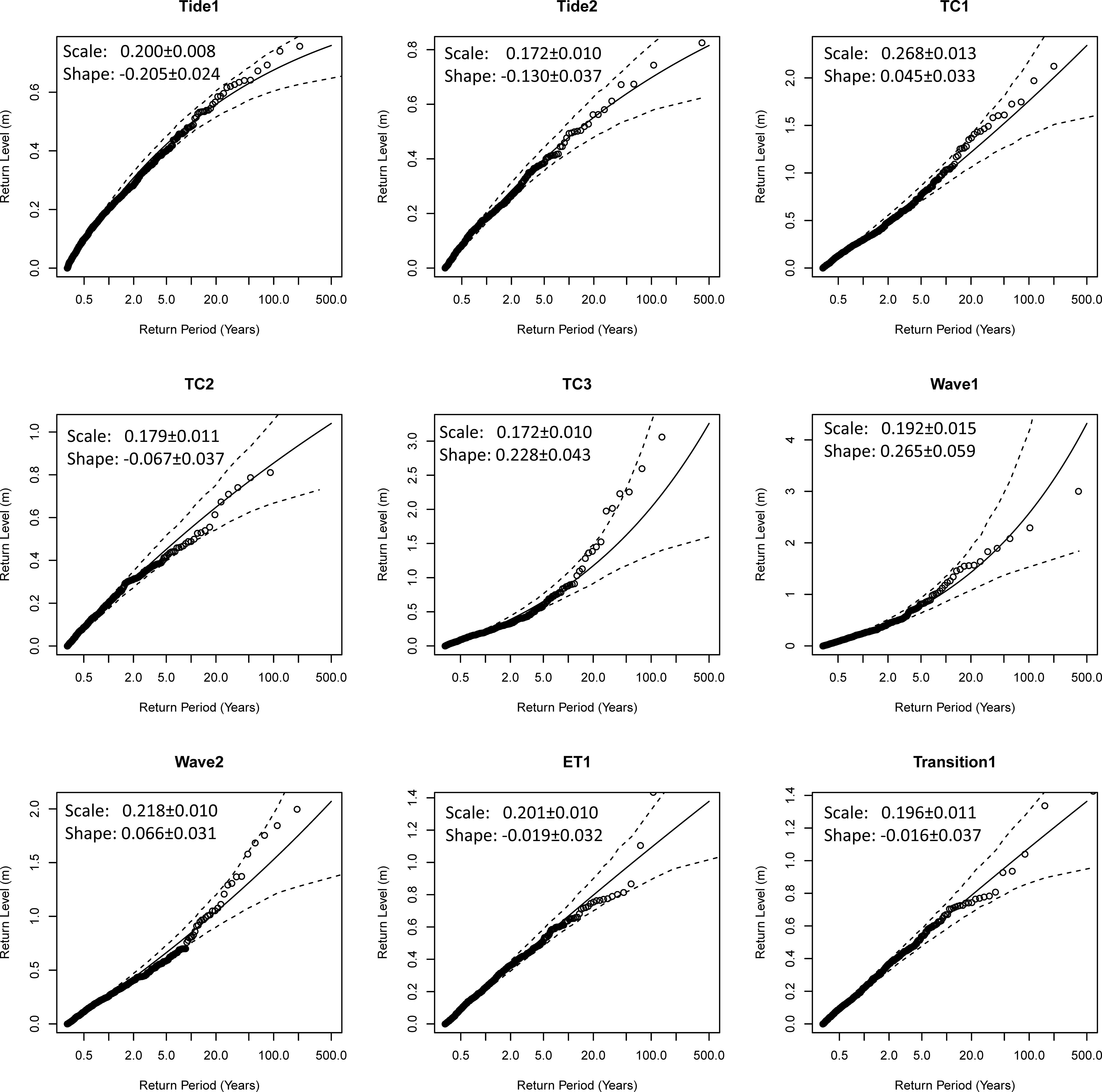
Figure 3. Normalized TG data and the regional extreme sea level (RESL) return level curves with 90% confidence intervals (5th and 95th% levels) as mapped in Figure 2. The y-axes are in meters above MHHW.

Factors affecting the fit of the regional models (Figure 3), and hence LESLs (Eq. 3) include methodological choices of the RFA local flood index (u), the threshold (also u in our case) or time block to assess local TG exceedances or block maxima and the extreme value distribution (e.g., GEV or GPD) fit to the regional data. As discussed by Wahl et al. (2017) for single-gauge analyzes, 100-year LESLs can vary by 10’s of centimeters in some unbounded locations depending upon methodological choices and the extreme value distribution used to fit TG data, though GPD fits to threshold exceedances are less likely to be biased high or low. Specific to the RFA is the selection of an optimal flood index as discussed by Weiss and Bernardara (2013) who show that RFA-based LESLs can vary (<10 cm per their GEV-based examples) depending upon regional heterogeneity and on the nature of treatment to the local flood index (e.g., using the mean or median value of annual maxima or threshold exceedances) used within a particular region. In both studies (Weiss and Bernardara, 2013; Wahl et al., 2017), nuances in model choice mostly affect the tail of the distribution (e.g., 100-year LESLs). Our usage of the TG exceedance threshold directly as the local flood index is the equivalent to the location parameter, which Weiss and Bernardara (2013) find as an optimal index in some circumstances and follows other studies (Roth et al., 2012; Frau et al., 2018).

For method consistency and application simplicity across all the Pacific study regions (Figure 2), we compute LESLs (i.e., Eq. 3) keeping to a constant definition of u (98th percentile of a TG’s 4-day declustered daily highest levels). However, we compute several sets of LESL results using alternate methods to estimate u values and their uncertainties (Eq. 4) and compare them to those based upon the entire TG record (Supplementary Table 1). These alternative methods may be of interest to coastal communities that are not co-located to a TG used in this study, but have predictions of tide range or have access to or be planning deployments to collect in situ water level records. Applicable for where tide range predictions exist, a set of LESLs are based upon predicted values of u and their uncertainties from an underlying linear dependence between tide range and u across the Pacific TGs (Figure 4A). The underlying high correlation between tide range and u (R² = 0.86 with a 0.074 m RMSE) is similar to findings of Merrifield et al. (2013) who found a high correlation between the range in water level variability and average annual highest water level. Two exceptions not included in the linear regression are Nome, Alaska (TG #595; Supplementary Table 1) and the Japanese coral atoll of Minamito (TG #49) that have extremely small tide ranges compared to their u values (>two standard deviation outliers).

FIGURE 4

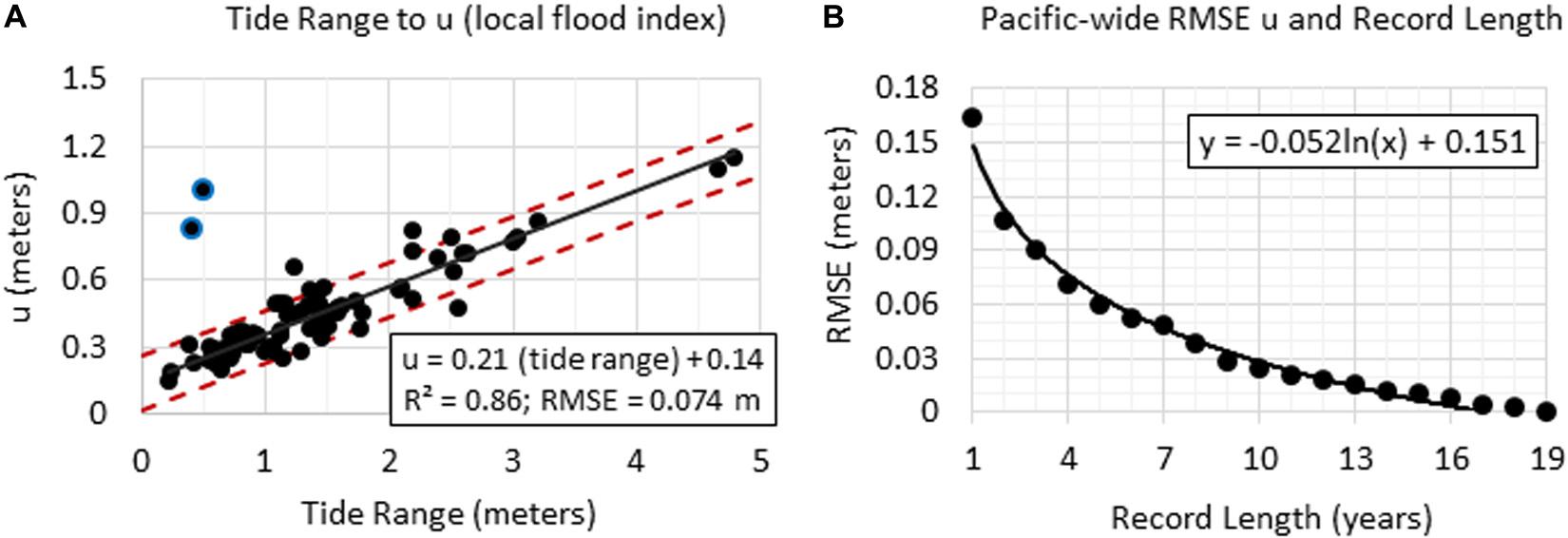
Figure 4. (A) Tide range and u (local RFA local flood index and TG exceedance threshold) and linear regression fit statistics with two outlier TGs (Nome and Minamito > 2 stdev) not included in the regression. In (B) is the root mean square error (RMSE) for estimates of u based upon 1–19 years of consecutive data over the 2001–2019 period based upon 64 of the 84 TGs used in this study.

Another set of LESLs are based upon u values estimated using short data records and utilize an uncertainty estimate (RMSE) in u which is record-length dependent (Figure 4B). For simplicity (as in Figure 4A), the RMSE in u is estimated across the entire Pacific study region (64 of 84 TGs included), but only those with complete 2001–2019 records and also excluding Ofunato (TG #351) and Yakutat (TG #570) due to significant non-linear vertical land motion in the time series. The RMSE as a function of consecutive record length is plotted in Figure 4B and fit using a best-fit logarithmic function. With about 4 years of data, the RMSE in u (7–8 cm) is about the same as those based upon the tide range (Figure 4A). After 19 years, the RMSE is about 1 cm (not shown), but has been reduced to zero across the 1–19 year range.

Our 1- and 100-year RFA LESLs (Figure 5) based upon record-length values of u (Supplementary Table 1) have median values of 0.47 and 0.83 m above MHHW, respectively. Higher 100-year LESLs (e.g., >1.2 m) generally occur along the continental margins where larger variability occurs from extreme astronomical tides or tropical and extratropical storm exposure such as is the case for Nagasaki, Townsville and Ketchikan (Table 1). In terms of the 1-year LESLs and higher probability events, a similar spatial pattern emerges, but tide range becomes more of a dominant factor as expressed by the tight coupling between u and tide range across the Pacific TG locations (Figure 4A). For example, smaller 1-year levels at Papeete, Honolulu and Guam (Table 1) occur largely in response to smaller tide ranges.

FIGURE 5

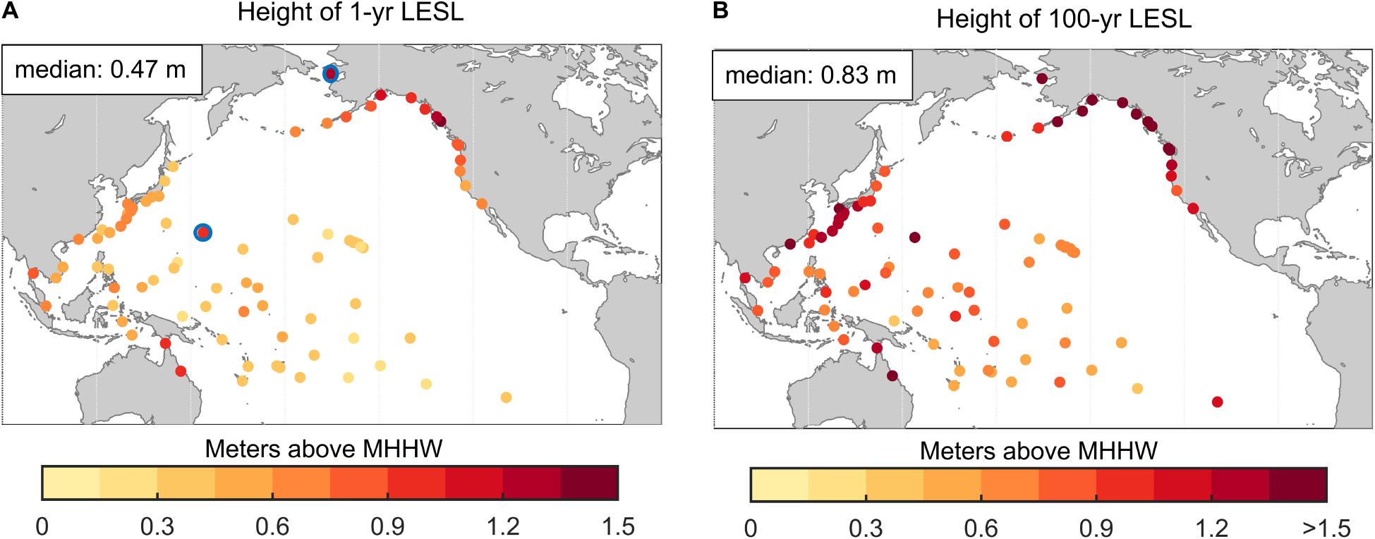
Figure 5. (A) 1-year and (B) 100-year LESLs with the two outlier TGs shown with blue circles. The “>” in the last tick label in the legend (in this figure and similarly in others) indicate at least one value exceeds 1.5 m.

TABLE 1

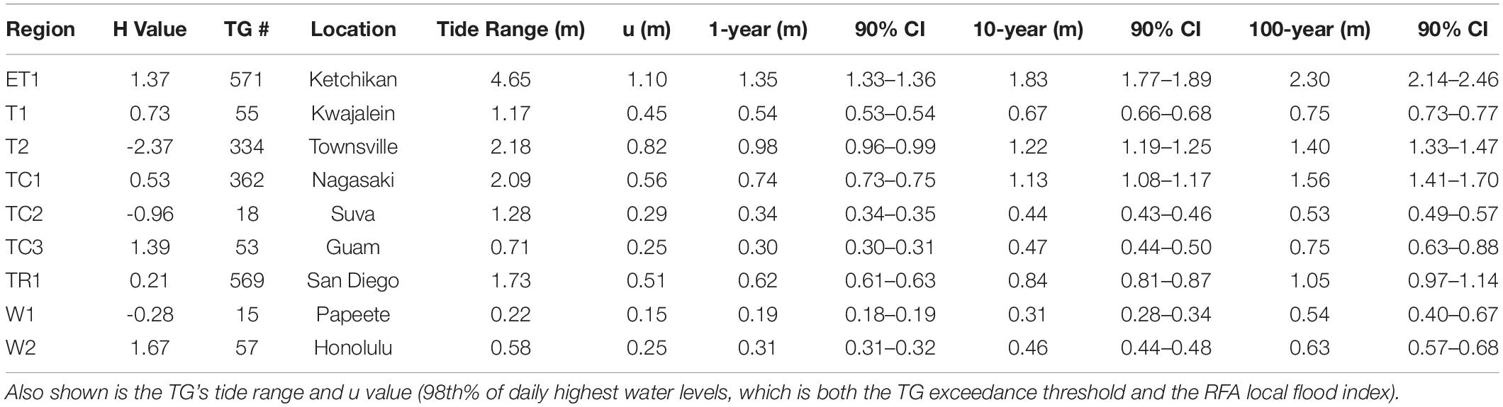
Table 1. An example of 1-, 10-, and 100-year return levels (meters above MHHW) with 90% confidence intervals (CI: spread of the 5th and 95th% levels) from regional frequency analysis (RFA) highlighting a subset of tide gauges (TG) within each homogeneous region and its H value.

Result Comparisons

When compared to a single-gauge GPD estimate of LESLs using the same TG data, the RFA-based LESLs show some important distinctions. At the 1-year LESL (Figure 6A), the two approaches yield similar results with RFA estimates only slightly higher (median value is 2 cm higher). However, the 100-year LESLs are very different (Figure 6B), with the RFA LESLs much higher in many locations (0.3–0.6 m) such as along the Japan and U.S. Pacific Northwest coastlines and 0.11 m higher overall (median value). In terms of a broad regional comparison (Figure 6C), the single-gauge LESLs are 87% of those from the RFA based upon linear regression coefficient (or RFA is about 13% higher), which about the ratio of the median of the single gauge (0.76 m) to RFA (0.83 m) 100-year LESLs. Higher LESLs is a typical artifact of the RFA (Hall et al., 2016) and a primary purpose of the RFA process–to quantify ESL probabilities and exposure locally from a regional perspective. There are a few exceptions where the RFA 100-year LESLs are much smaller (∼1 m, Figure 6B), e.g., Nome, which may be partly attributed to its short record length (bias) of 23 years (Supplementary Table 1).

FIGURE 6

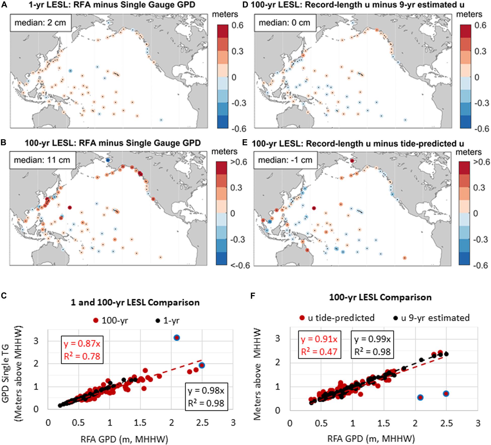
Figure 6. Differences in the RFA LESLs and those computed using a single TG only at the (A) 1-year and (B) 100-year levels and (C) linear regression between the sets in (A,B). Mapped differences in the 100-year LESLs using record length u and (D) 9-year (2011–2019) estimates and (E) a tide-range based predictions of u plotted with linear regression statistics in (F). The outliers (blue circles) are included in the regressions in plot (C,F).

Sensitivity of LESLs localized by various methods to estimate u are the focus of Figures 6D–F. Comparisons between the RFA 100-year LESLs and those with u values from 9 years of data (2011–2019, which is an arbitrary record length, but represents half of a tidal nodal cycle) and predicted by tide range (Figures 6D,F, respectively) reveal little inherent bias with (median) differences of ≤1 cm. Linear regression shows a tight coupling (R² = 0.98) between the LESLs based upon record-length and 9-year estimates of u (Figure 6F). Differences using a tide-range predicted u (Figure 6E) are more pronounced due to its underlying predictive relationship (Figure 4A), with the two outliers (Nome and Minamito) >1 m apart and reducing the overall goodness-of-fit (Figure 6F; R² = 0.47).

Comparison of the spread in 100-year 90% confidence intervals (Figure 7) show that the (median) RFA LESLs spread is 14 cm (Figure 7A) and is 8 cm tighter (Figure 7B; negative values illustrate where RFA values are less) than those based upon a single-gauge (GPD) analysis. The locations with much tighter (<-0.6 m) RFA 100-year 90% confidence intervals are mostly within regions prone to rare (outlier) extremes and with unbounded tails (positive shape parameters in Figure 3), namely TC Regions 1 and 3 and Wave Regions 1 and 2. Comparison of the 100-year 90% confidence intervals using u predicted by tide range as the local index flood (Figure 7C) shows the additional inflation due to method uncertainty (Eq. 4), which is persistent spatially (median difference of -0.35 m). Of note is that some of the location-specific peculiarities are less than those based upon a single-gauge approach (Figure 7B) due to the RFA process (standard deviation of 10 vs. 34 cm by single-gauge estimate). The inflation in the 100-year 90% confidence interval when using a 9-year estimate of u (Figure 7D) is less than those from a tide-range predicted u (Figure 7C) and closer to those using u values based upon the complete TG record (median difference = -0.09 m in Figure 7D).

FIGURE 7

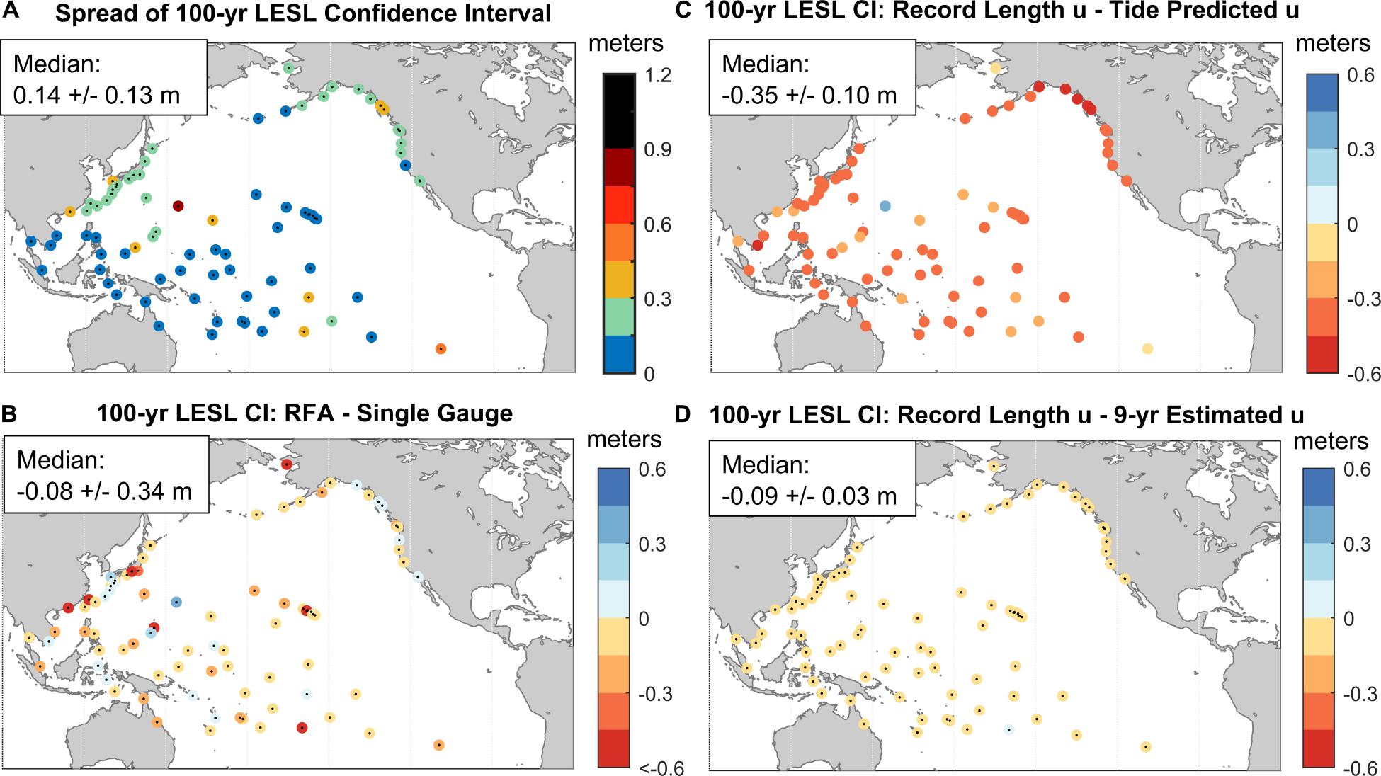
Figure 7. The spread of the 100-year LESL 90% confidence interval using (A) the RFA values and the differences with those computed using (B) a single TG GPD analysis, (C) RFA estimates predicted from tide range (Figure 4A) and (D) 9-year estimates of u (Figure 4B).

The RFA LESLs are next compared to recent foundational sets of LESLs derived from both TGs and advanced tide and storm surge modeling. A comparison in Figure 8 is made to the results of a single-gauge GPD analysis (Rasmussen et al., 2018) that are closely aligned (similar methodology and results) to those supporting the IPCC Global Warming of 1.5°C (Hoegh-Guldberg et al., 2018) and SROCC (Oppenheimer et al., 2019) assessments. The comparison with Rasmussen et al. (2018) results is made at 61 of the 84 TGs in our study. The RFA 1- and 100-year LESLs are both higher overall, by about 10 and 16%, respectively based upon linear regression (Figure 8A). For context, the median (±1 SD) TG difference of the 1- and 100-year LESLs being compared in Figure 8A is 0.06 and 0.15 m (±0.07 and 0.26 m), respectively, with the higher values from the RFA LESLs. Comparison of a 100-year LESLs based on a single-gauge GPD analysis using data in this study (e.g., same data set compared in Figure 6B) to the Rasmussen et al. (2018) are quite similar as would be expected since both use the same data set (regression slope of 1.01; not shown).

FIGURE 8

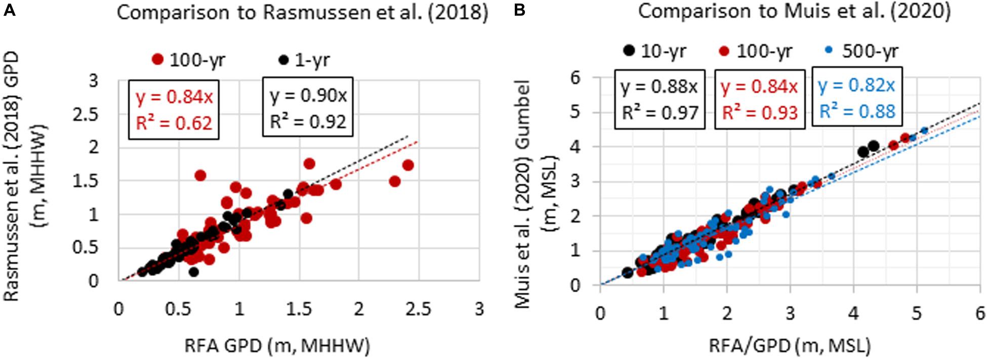
Figure 8. Comparison of our RFA GPD (A) 1- and 100-year LESLs to those from a single-gauge GPD of Rasmussen et al. (2018) and (B) 10-, 100-, and 500-year LESLs to those with a Gumbel fit for global tide and surge model output of Muis et al. (2020) with linear regression fit and statistics.

LESLs are also compared to those from a third-generation global tide and surge model forced by ERA5 climate reanalysis from 1979 to 2017 (Muis et al., 2020). The RFA LESLs, once adjusted to a comparable mean sea level datum, are also higher overall to the modeled results of Muis et al. (2020), who fit a Gumbel distribution to the annual maxima (Figure 8B). Comparing the 10-, 100-, and 500-year LESLs at 74 of the 84 TGs, the RFA estimates are about 12, 16, and 18% higher based upon linear regression with good agreement (small variability) between the two sets of results (R² of 0.97, 0.93, 0.88), respectively (Figure 8B). For context, the median (±1 SD) differences are 0.20, 0.25, and 0.31 m (±0.14, 0.21, 0.30 m), respectively. The RFA result comparison to Muis et al. (2020) could also reflect inherent differences in data utilization (threshold exceedances vs. annual maxima) and fitted extreme value distribution (GPD vs. Gumbel) and not necessarily model biases (Wahl et al., 2017). However, the large discrepancies between results, even down to the 2-year LESL (median difference of 0.17 m, not shown), would suggest some underlying response and/or possible tidal datum bias.

A Damaging Flood Threshold and Its Current Risk

Local flood risk varies according to many factors such as elevation, topography, urbanization and flood proofing. Instead of using probabilistic thresholds like the 100-year LESL (e.g., Oppenheimer et al., 2019), which may or may not cause significant or even noticeable impacts, we utilize NOAA’s flood severity thresholds. Following methods of Sweet et al. (2018), we first regionalize all TGs with NOAA minor flood thresholds along U.S. Pacific coastlines (Figure 9A; median value of 0.58 m above MHHW) and then plot relative to tide range (Figure 9B) as the initial basis for deriving a Pacific Basin flood threshold/infrastructure vulnerability definition. NOAA-defined minor flooding typically is more disruptive (e.g., flooding of some roadways, stormwater system infiltration), whereas NOAA-defined moderate flooding is damaging to public and private infrastructure. When a moderate (and/or major) flood is imminent, NOAA issues a coastal flood warning for conditions posing a serious risk to life and property (Sweet et al., 2018). To define a moderate flood threshold throughout the Pacific Basin (henceforth called a damaging flood), we add 0.3 m to this quadratic fit/threshold, which is about the median offset between the U.S. NOAA minor and moderate flood thresholds (Sweet et al., 2018) and apply this relationship at all TGs within our study. We do this because there are many more TGs with NOAA minor flood thresholds than with NOAA moderate threshold defined along the U.S. Pacific coastline. An important distinction between this study’s approach broadly defining infrastructure flood thresholds and that of Sweet et al. (2018) is the inclusion of Alaska NOAA thresholds and the usage of a quadratic fit.

FIGURE 9

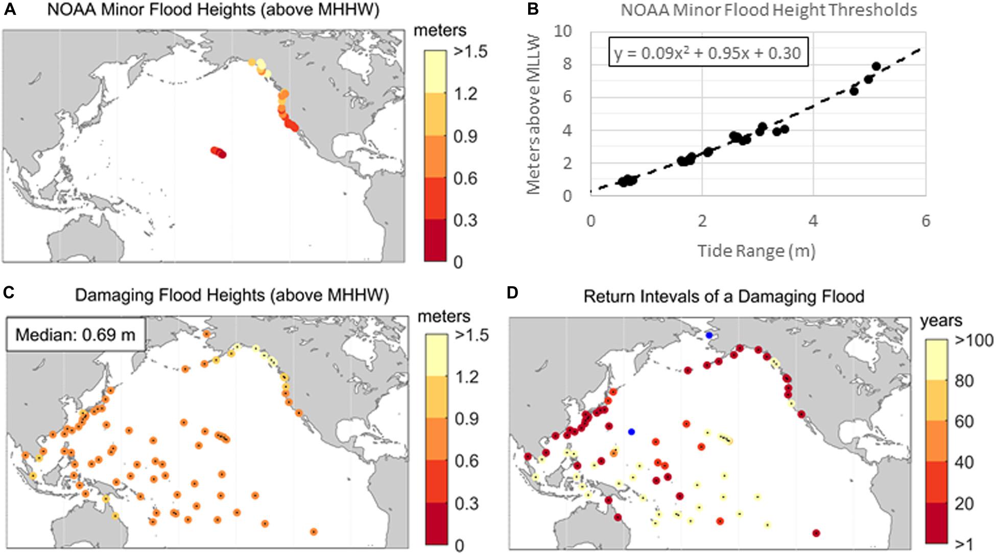
Figure 9. (A) NOAA coastal thresholds for minor flooding along U.S. Pacific coastlines, (B) regression of NOAA minor flood threshold heights along Pacific coastlines shown in (A) with tide range, (C) proposed heights of a Pacific damaging flood level (minor flood threshold +0.3 m) at TGs in this study and (D) return intervals of the damaging flood level based upon the RFA LESLs. The two outlier TGs in blue have return intervals less than 0.1 years.

Applying this definition across our study’s TGs, the median height of the Pacific damaging flood threshold is 0.69 m above MHHW and spans from about 0.6 and 1.2 m above MHHW (Figure 9C) depending upon local tide range. As a whole, damaging floods have a median (not shown) return interval (Figure 9D) of about 20–25 years, which equates to about a 4–5% annual chance of occurring. Longer return intervals (i.e., >100 years) occur where extreme variability is less (where LESL probabilities tend to be bounded: Figure 3) and there is a spatial pattern resembling that of the heights of the 100-year LESLs (Figure 5B). At the two outlier TGs where non-tidal variability is relatively extreme (Figure 4A), damaging floods occur >10 times per year (blue dots in Figure 9D) and local vulnerability and impacts are likely not adequately defined by this threshold level. For context, a damaging flood in Honolulu is defined here as 0.66 m above MHHW (Figure 9C), which is 0.3 m higher than the regression fit to NOAA minor flood heights along Pacific coastlines (Figure 9B) that locally cause impacts (Habel et al., 2020), 0.03 m higher than its RFA 100-year LESL, and about 0.24 m higher than the 100-year LESL quantified using a single-gauge GPD analysis (Figure 1A).

Future Flood Risk

To quantify future risk of a damaging flood event, the median RSL projections of RCP4.5 developed under the IPCC SROCC (Oppenheimer et al., 2019), which equate to about a 0.5 m global rise by 2100 are used with our LESL probabilities. We note that the 1983–2001 reference frame is about the same as the RSL projection baseline (1986–2005). Under such a scenario and assuming flood defenses do not change, by 2055 (Figure 10A), the damaging flood level is (median value) only 0.44 m above MHHW and occurs about once/year (median value). This finding is supportive of the findings of Oppenheimer et al. (2019), though their metric to assess flood risk is their 100-year LESL, which is generally less than our RFA LESLs (e.g., as in Honolulu, Figure 1A). Damaging floods in 2055 are projected to occur less often along many island coastlines (dark blue dots in Figure 10A) where flood levels have contemporary return intervals closer to the 100-year level (Figure 9D). By 2100, the damaging flood level is only 0.14 m above MHHW (median value) and events occur more than 10 times/year in most locations (Figure 10B).

FIGURE 10

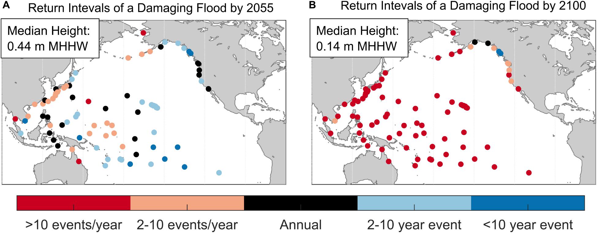
Figure 10. Change in return intervals of a damaging flood in (A) 2055 and by (B) 2100 under median RSL projections of the SROCC RCP4.5.

Summary Remarks

The risk of disruptive-to-destructive flooding (e.g., from “king tides” to tropical cyclone storm surge) is a serious concern within Pacific Basin coastal communities (Keener et al., 2018). Especially in light of rising seas, there is a need for data and mapped (e.g., Figure 1) information regarding current and future LESL probabilities along all populated coastlines—not just where TGs exist—for planning and preparedness purposes. Modeling and reanalysis of storm tides can help spatially granulate LESL probabilities, but their results often do not capture the response (e.g., surge/set up) peculiarities in some locations, especially those exposed to tropical cyclones. Even where TGs exist, measurements often are not long enough to capture historically significant events at a particular location or miss those completely that are of regional significance. Regional aggregation of TG data via the RFA process and its ability to support localization of RESL probabilities is a method that can help in both regards. Here, we suggest usage of short-term water level observations (either existing or future efforts) or tide-range information to augment estimates of LESL probabilities and flood risk for Pacific coastal communities without long-term TG observations. Ideally, output from high-resolution tide models would be employed to localize the RESLs and produce high-resolution LESLs estimates along coastlines.

A consequence of the RFA’s data aggregation is that uncertainties of low-probability LESLs are better constrained (i.e., narrower 90% confidence interval) and their magnitudes are generally higher. This is particularly important from the perspective of an individual TG location where rare (outlier) events may be a (hidden) threat since occurrences are under-sampled. Using a RFA, the probability of occurrence for the same water level is more probable than recognized by conventional (single gauge or dynamical model) statistics. By extension, the risk of consequential flooding along Pacific coastlines is also likely under-estimated by these same conventional methods. There may be locations that due to topography and/or coastline orientation are afforded some level of natural protection and the RFA process produces a positive bias in LESL estimates.

Narrower confidence intervals of the RFA, though implying greater precision, do not necessarily imply greater accuracy. Accuracy measures such as reduced high or low bias of LESL probabilities from GPD fits (Wahl et al., 2017) and minimizing record-length biases and regionalizing risk through the RFA process, however, would suggest that the RFA results are more accurate than those from single-gauge analysis or a 40–50 year reanalysis from dynamical storm-tide modeling. In a practical sense, the storm surge associated with Hurricane Iniki in 1992, which caused record-setting water levels along the Hawaiian Island of Kauai (e.g., 0.96 m above MHHW at Nawiliwili: TG #58) offers a lens to evaluate the robustness of results. By chance, this hurricane narrowly missed Oahu Island and the nearby TG in Honolulu (TG #57) where water levels were more than a 0.5 m less (about 0.41 m above MHHW). From a probabilistic standpoint, Hurricane Iniki’s water levels represent about a 5-year and a 100-year LESL at Honolulu (Figure 1 and Table 1) and are about 0.1 and 0.25 m above the 500-year LESL 90% confidence interval at Nawiliwili from a RFA and both a single-gauge analysis/storm-tide reanalysis, respectively. Though this event and its surge are still an outlier, its occurrence is captured via the RFA process and transferred to all TGs across the Hawaiian Islands. We would argue that the results from the RFA process, if not more accurate, are a more sensible result for risk management and robust decision making under current and future LESLs (Hall et al., 2016).

LESL event probabilities themselves do not necessarily imply a certain severity of damage or impacts, although the 100-year event is a common proxy for severe or consequential flooding (Oppenheimer et al., 2019). Instead, a height threshold is proposed for a damaging flood to broadly establish infrastructure vulnerabilities along the Pacific Basin (Figure 9C). The height for a damaging flood varies according to the underlying relationship between tide range and NOAA coastal flood severity thresholds along the U.S. Pacific coastline used for weather impact forecasting and communication purposes. Along U.S. coastlines, NOAA moderate (damaging) floods pose a serious risk to life and property. As defined for the Pacific Basin region in this study, damaging floods currently have about a (median value) 20–25 year return interval (4–5% annual chance). However, that risk continues to grow with RSL rise. In fact, damaging floods are likely to occur on an annual basis in the next 35 years (2055) considering RCP4.5 projections at a majority of TGs if flood defenses or other adaptive measures are not enacted. They will become a common occurrence (>10 events/year) by 2100 largely in response to tidal forcing alone as the gap or freeboard between average high tide and damaging flood levels closes.

One flood risk threshold does not fit all circumstances and other locally important thresholds should be examined as appropriate. Likewise, no one model will definitively provide the “true probability” of rare and often-compounding events leading to damaging floods. As discussed here, a host of factors can affect estimates of rare-event probabilities (e.g., the 100-year LESL), but methodological differences may be indistinguishable relative to the uncertainties imposed by mapping for decision-support purposes (Kulp and Strauss, 2019)³. On the other hand, most extreme value model estimates converge and their uncertainties close at the higher probability portion of the distribution nearing the annual (1-year) event. In this context, and with knowledge of a realistic damaging flood height threshold, an examination of remaining freeboard can be made and future projections of its loss under RSL projections leading to chronic flooding can be performed with relative certainty. A strength of the RFA approach is the ability to spatially define LESLs across regions affording coastal communities with or without long-term TGs tools they need to assess current flood risk and make informed decisions in the face of RSL rise and an uncertain future.

Data Availability Statement

Publicly available datasets were analyzed in this study. This data can be found at the University of Hawaii Sea Level Center (https://uhslc.soest.hawaii.edu/datainfo/).

Author Contributions

WS, AG, and JO were responsible for data processing and analysis. WS wrote the manuscript, with contributions from AG, JO, and JM. All authors contributed to the article and approved the submitted version.

Funding

Support was provided from the US Department of Defense (DoD) Strategic Environmental Research and Development Program (SERDP) through work carried out under Project RC-2644.

Conflict of Interest

The authors declare that the research was conducted in the absence of any commercial or financial relationships that could be construed as a potential conflict of interest.

Supplementary Material

The Supplementary Material for this article can be found online at: https://www.frontiersin.org/articles/10.3389/fmars.2020.581769/full#supplementary-material

Footnotes

1. ^ https://tidesandcurrents.noaa.gov/tide_predictions.html
2. ^ https://water.weather.gov/ahps/
3. ^ https://coast.noaa.gov/slr/#/layer/slr

References

Bardet, L., Duluc, C. M., Rebour, V., and L’her, J. (2011). Regional frequency analysis of extreme storm surges along the French coast. Nat. Hazards Earth Syst. Sci. 11, 1627–1639. doi: 10.5194/nhess-11-1627-2011

CrossRef Full Text | Google Scholar

Bernardara, P., Andreewsky, M., and Benoit, M. (2011). Application of regional frequency analysis to the estimation of extreme storm surges. J. Geophys. Res. 116:C02008. doi: 10.5194/nhess-11-1627-2011

CrossRef Full Text | Google Scholar

Buchanan, M. K., Oppenheimer, M., and Kopp, R. E. (2017). Amplification of flood frequencies with local sea level rise and emerging flood regimes. Environ. Res. Lett. 12:064009. doi: 10.1088/1748-9326/aa6cb3

CrossRef Full Text | Google Scholar

Calafat, F. M., and Marcos, M. (2020). Probabilistic reanalysis of storm surge extremes in Europe. Proc. Natl. Acad. Sci. U.S.A. 117, 1877–1883. doi: 10.1073/pnas.1913049117

PubMed Abstract | CrossRef Full Text | Google Scholar

Carreau, J., Naveau, P., and Neppel, L. (2017). Partitioning into hazard subregions for regional peaks-over-threshold modeling of heavy precipitation. Water Resour. Res. 53, 4407–4426. doi: 10.1002/2017wr020758

CrossRef Full Text | Google Scholar

Church, J. A., Clark, U., Cazenave, A., Gregory, J. M., Jevrejeva, S., Levermann, A., et al. (2013). “Sea Level Change,” in Climate Change 2013: The Physical Science Basis. Contribution of Working Group I to the Fifth Assessment Report of the Intergovernmental Panel on Climate Change, eds T. F. Stocker, D. Qin, G.-K. Plattner, M. Tignor, S. K. Allen, J. Boschung, et al. (Cambridge: Cambridge University Press), 1137–1216.

Google Scholar

Coles, S., and Dixon, M. (1999). Likelihood-based inference for extreme value models. Extremes 2, 5–23. doi: 10.1023/A:1009905222644

CrossRef Full Text | Google Scholar

Coles, S. G. (2001). An Introduction to Statistical Modeling of Extreme Values. London: Springer, 208.

Google Scholar

Dalrymple, T. (1960). Flood Frequency Analysis. U.S. Geological Survey Water-Supply Paper 1543-A. Washington, D.C: U.S. Government Printing Office.

Google Scholar

Frau, R., Andreewsky, M., and Bernardara, P. (2018). The use of historical information for regional frequency analysis of extreme skew surge. Nat. Hazards Earth Syst. Sci. 18, 949–962. doi: 10.5194/nhess-18-949-2018

CrossRef Full Text | Google Scholar

Frederikse, T., Buchanan, M. K., Lambert, E., Kopp, R. E., Oppenheimer, M., Rasmussen, D. J., et al. (2020). Antarctic Ice Sheet and emission scenario controls on 21st-century extreme sea-level changes. Nat. Commun. 11, 1–11. doi: 10.1029/ar077p0001

CrossRef Full Text | Google Scholar

Ghanbari, M., Arabi, M., Obeysekera, J., and Sweet, W. (2019). A coherent statistical model for coastal flood frequency analysis under nonstationary sea level conditions. Earth’s Future 7, 162–177. doi: 10.1029/2018ef001089

CrossRef Full Text | Google Scholar

Habel, S., Fletcher, C. H., Anderson, T. R., and Thompson, P. R. (2020). Sea-Level Rise induced Multi-Mechanism flooding and contribution to Urban infrastructure failure. Sci. Rep. 10, 1–12.

Google Scholar

Haigh, I. D., MacPherson, L. R., Mason, M. S., Wijeratne, E. M. S., Pattiaratchi, C. B., Crompton, R. P., et al. (2014a). Estimating present day extreme water level exceedance probabilities around the coastline of Australia: tropical cyclone-induced storm surges. Clim. Dyn. 42, 139–157. doi: 10.1007/s00382-012-1653-0

CrossRef Full Text | Google Scholar

Haigh, I. D., Wijeratne, E. M. S., MacPherson, L. R., Pattiaratchi, C. B., Mason, M. S., Crompton, R. P., et al. (2014b). Estimating present day extreme water level exceedance probabilities around the coastline of Australia: tides, extra-tropical storm surges and mean sea level. Clim. Dyn. 42, 121–138. doi: 10.1007/s00382-012-1652-1

CrossRef Full Text | Google Scholar

Hall, J. A., Gill, S., Obeysekera, J., Sweet, W., Knuuti, K., and Marburger, J. (2016). Regional Sea Level Scenarios for Coastal Risk Management: Managing the Uncertainty of Future Sea Level Change and Extreme Water Levels for Department of Defense Coastal Sites Worldwide. Virginia: U.S. Department of Defense, 224.

Google Scholar

Hall, J. A., Weaver, C. P., Obeysekera, J., Crowell, M., Horton, R. M., Kopp, R. E., et al. (2019). Rising sea levels: helping decision-makers confront the inevitable. Coast. Manag. 47, 127–150. doi: 10.1080/08920753.2019.1551012

PubMed Abstract | CrossRef Full Text | Google Scholar

Hamlington, B. D., Fasullo, J. T., Nerem, R. S., Kim, K. Y., and Landerer, F. W. (2019). Uncovering the pattern of forced sea level rise in the satellite altimeter record. Geophys. Res. Lett. 46, 4844–4853. doi: 10.1029/2018gl081386

CrossRef Full Text | Google Scholar

Hoegh-Guldberg, O., Jacob, D., Taylor, M., Bindi, M., Brown, S., Camilloni, I., et al. (2018). Impacts of 1.5°C Global Warming on Natural and Human Systems. Global Warming of 1.5 C°C. An IPCC Special Report.

Google Scholar

Hosking, J. R. M. (2012). Towards statistical modeling of tsunami occurrence with regional frequency analysis. J. Math Ind. 4, 41–48.

Google Scholar

Hosking, J. R. M., and Wallis, J. R. (1997). Regional Frequency Analysis: An Approach Based on L-Moments. Cambridge: Cambridge Univ. Press.

Google Scholar

Hunter, J. (2012). A Simple Technique for Estimating an Allowance for Uncertain Sea-Level Rise. Clim. Change 113, 239–252. doi: 10.1007/s10584-011-0332-1

CrossRef Full Text | Google Scholar

IPCC (2014). “Climate change 2014: synthesis report,” in Contribution of Working Groups I, II and III to the Fifth Assessment Report of the Intergovernmental Panel on Climate Change, eds Core Writing Team, R. K. Pachauri and L. A. Meyer (Geneva: IPCC), 151.

Google Scholar

Keener, V., Helweg, D., Asam, S., Balwani, S., Burkett, M., Fletcher, C., et al. (2018). “Hawai‘i and U.S.-affiliated pacific Islands,” in Impacts, Risks, and Adaptation in the United States: Fourth National Climate Assessment, Vol. II, eds D. R. Reidmiller, C. W. Avery, D. R. Easterling, K. E. Kunkel, K. L. M. Lewis, T. K. Maycock, et al. (Washington, DC: U.S. Global Change Research Program), 1242–1308. doi: 10.7930/NCA4.2018.CH27

CrossRef Full Text | Google Scholar

Kopp, R. E., Gilmore, E. A., Little, C. M., Lorenzo-Trueba, J., Ramenzoni, V. C., and Sweet, W. V. (2019). Usable science for managing the risks of sea-level rise. Earth’s Future 7, 1235–1269. doi: 10.1029/2018ef001145

PubMed Abstract | CrossRef Full Text | Google Scholar

Kopp, R. E., Hay, C. C., Little, C. M., and Mitrovica, J. X. (2015). Geographic variability of sea-level change. Curr. Clim. Change Rep. 1, 192–204. doi: 10.1007/s40641-015-0015-5

CrossRef Full Text | Google Scholar

Kopp, R. E., Horton, R. M., Little, C. M., Mitrovica, J. X., Oppenheimer, M., Rasmussen, D. J., et al. (2014). Probabilistic 21st and 22nd century sea-level projections at a global network of tide- gauge sites. Earth’s Future 2, 383–406. doi: 10.1002/2014ef000239

CrossRef Full Text | Google Scholar

Kulp, S. A., and Strauss, B. H. (2019). New elevation data triple estimates of global vulnerability to sea-level rise and coastal flooding. Nat. Commun. 10, 1–12.

Google Scholar

Le Cozannet, G., Nicholls, R. J., Hinkel, J., Sweet, W. V., McInnes, K. L., Van de Wal, R. S., et al. (2017). Sea level change and coastal climate services: the way forward. J. Mar. Sci. Eng. 5:49. doi: 10.3390/jmse5040049

CrossRef Full Text | Google Scholar

Lin, N., Emanuel, K., Oppenheimer, M., and Vanmarcke, E. (2012). Physically based assessment of hurricane surge threat under climate change. Nat. Clim. Change 2, 462–467. doi: 10.1038/Nclimate1389

CrossRef Full Text | Google Scholar

Lin, N., Marsooli, R., and Colle, B. (2019). Storm surge return levels induced by the mid-to-late-twenty-first-century extratropical cyclones in the Northeastern United States. Clim. Change 154, 143–158. doi: 10.1007/s10584-019-02431-8

CrossRef Full Text | Google Scholar

Lobeto, H., Menendez, M., and Losada, I. J. (2018). Toward a methodology for estimating coastal extreme sea levels from satellite altimetry. J. Geophys. Res. 123, 8284–8298. doi: 10.1029/2018jc014487

CrossRef Full Text | Google Scholar

Menéndez, M., and Woodworth, P. L. (2010). Changes in extreme high water levels based on a quasi-global tide-gauge data set. J. Geophys. Res. 115:C10011. doi: 10.1029/2009JC005997

CrossRef Full Text | Google Scholar

Merrifield, M. A., Genz, A. S., Kontoes, C. P., and Marra, J. J. (2013). Annual maximum water levels from tide gauges: contributing factors and geographic patterns. J. Geophys. Res. Oceans 118, 2535–2546. doi: 10.1002/jgrc.20173

CrossRef Full Text | Google Scholar

Michele, C. D., and Rosso, R. (2001). Uncertainty assessment of regionalized flood frequency estimates. J. Hydrol. Eng. 6, 453–459. doi: 10.1061/(asce)1084-0699(2001)6:6(453)

CrossRef Full Text | Google Scholar

Moftakhari, H. R., AghaKouchak, A., Sanders, B. F., and Matthew, R. A. (2017). Cumulative hazard: the case of nuisance flooding. Earth’s Future 5, 214–223. doi: 10.1002/2016ef000494

CrossRef Full Text | Google Scholar

Mood, A., Graybill, F. A., and Boes, D. C. (1974). Introduction to the Theory of Statistics. New York, NY: McGraw-Hill.

Google Scholar

Muis, S., Apecechea, M. I., Dullaart, J., de Lima Rego, J., Madsen, K. S., Su, J., et al. (2020). A High-resolution global dataset of extreme sea levels, tides, and storm surges, including future projections. Front. Mar. Sci. 7:263. doi: 10.3389/fmars.2020.00263

CrossRef Full Text | Google Scholar

Muis, S., Verlaan, M., Winsemius, H. C., Aerts, J. C., and Ward, P. J. (2016). A global reanalysis of storm surges and extreme sea levels. Nat. Commun. 7, 1–12.

Google Scholar

Nadal-Caraballo, N. C., Melby, J. A., Gonzalez, V. M., and Cox, A. T. (2015). Coastal storm hazards from Virginia to Maine (No. ERDC/CHL-TR-15-5). Vicksburg, MS: Engineer research and development center.

Google Scholar

NOAA (2003). Computational Techniques for Tidal Datums Handbook. NOAA Special Publication NOS CO-OPS 2. Silver Spring, MA: U.S. Department of Commerce.

Google Scholar

Oppenheimer, M., Glavovic, B. C., Hinkel, J., van de Wal, R., Magnan, A. K., Abd-Elgawad, A., et al. (2019). “Sea level rise and implications for low-lying islands, coasts and communities,” in IPCC Special Report on the Ocean and Cryosphere in a Changing Climate, eds H.-O. Pörtner, D. C. Roberts, V. Masson-Delmotte, P. Zhai, M. Tignor, E. Poloczanska, et al.

Google Scholar

Perica, S., Pavlovic, S., St Laurent, M., Trypaluk, C., Unruh, D., and Wilhite, O. (2018). Precipitation-Frequency Atlas of the United States. Texas: Version 2.0, 11. Silver Spring, MD: National Oceanic and Atmospheric Administration, National Weather Service.

Google Scholar

Rasmussen, D. J., Bittermann, K., Buchanan, M. K., Kulp, S., Strauss, B. H., Kopp, R. E., et al. (2018). Extreme sea level implications of 1.5 C, 2.0 C, and 2.5 C temperature stabilization targets in the 21st and 22nd centuries. Environ. Res. Lett. 13:034040. doi: 10.1088/1748-9326/aaac87

CrossRef Full Text | Google Scholar

Roth, M., Buishand, T. A., Jongbloed, G., Klein Tank, A. M. G., and Van Zanten, J. H. (2012). A regional peaks-over-threshold model in a nonstationary climate. Water Resour. Res. 48:W11533.

Google Scholar

Rueda, A., Vitousek, S., Camus, P., Tomás, A., Espejo, A., Losada, I. J., et al. (2017). A global classification of coastal flood hazard climates associated with large-scale oceanographic forcing. Sci. Rep. 7, 1–8.

Google Scholar

Smith, A., Sampson, C., and Bates, P. (2015). Regional flood frequency analysis at the global scale. Water Resour. Res. 51, 539–553. doi: 10.1002/2014WR015814

CrossRef Full Text | Google Scholar

Sweet, W. V., Dusek, G., Carbin, G., Marra, J. J., Marcy, D., and Simon, S. (2020). 2019 State of US High Tide Flooding With a 2020 Outlook. NOAA Tech. Rep. NOS CO-OPS., Vol. 92. Silver Spring, MD: National Oceanic and Atmospheric Administration, 17.

Google Scholar

Sweet, W., Dusek, G., Obeysekera, J., and Marra, J. (2018). Patterns and Projections of High Tide Flooding Along the U.S. Coastline using a Common Impact Threshold. NOAA Technical Report NOS CO-OPS, Vol. 86., Silver Spring, MD: National Oceanic and Atmospheric Administration.

Google Scholar

Sweet, W. V., and Park, J. (2014). From the extreme and the mean: acceleration and tipping point of coastal inundation from sea level rise. Earth Futures 2, 579–600. doi: 10.1002/2014EF000272

CrossRef Full Text | Google Scholar

Taherkhani, M., Vitousek, S., Barnard, P. L., Frazer, N., Anderson, T. R., and Fletcher, C. H. (2020). Sea-level rise exponentially increases coastal flood frequency. Sci. Rep. 10, 1–17.

Google Scholar

Tebaldi, C., Strauss, B. H., and Zervas, C. E. (2012). Modelling sea level rise impacts on storm surges along US coasts. Environ. Res. Lett. 7:014032. doi: 10.1088/1748-9326/7/1/014032

CrossRef Full Text | Google Scholar

Thompson, P. R., Widlansky, M. J., Leuliette, E., Sweet, W., Chambers, D. P., Hamlington, B. D., et al. (2019). Sea level variability and change [in “State of the Climate in 2018”]. Bull. Amer. Meteor. Soc. 100, S181–S185. doi: 10.1175/2019BAMSStateoftheClimate.1

CrossRef Full Text | Google Scholar

Vitousek, S., Barnard, P. L., Fletcher, C. H., Frazer, N., Erikson, L., and Storlazzi, C. D. (2017). Doubling of coastal flooding frequency within decades due to sea-level rise. Sci. Rep. 7, 1–9.

Google Scholar

Vousdoukas, M. I., Mentaschi, L., Voukouvalas, E., Verlaan, M., Jevrejeva, S., Jackson, L. P., et al. (2018). Global probabilistic projections of extreme sea levels show intensification of coastal flood hazard. Nat. Commun. 9, 1–12.

Google Scholar

Wahl, T., Haigh, I. D., Nicholls, R. J., Arns, A., Dangendorf, S., Hinkel, J., et al. (2017). Understanding extreme sea levels for broad-scale coastal impact and adaptation analysis. Nat. Commun. 8, 1–12. doi: 10.2112/jcoastres-d-12-00127.1

CrossRef Full Text | Google Scholar

Weiss, J., and Bernardara, P. (2013). Comparison of local indices for regional frequency analysis with an application to extreme skew surges. Water Resour. Res. 49, 2940–2951. doi: 10.1002/wrcr.20225

CrossRef Full Text | Google Scholar

Weiss, J., Bernardara, P., and Benoit, M. (2014). Formation of homogeneous regions for regional frequency analysis of extreme significant wave heights. J. Geophys. Res. 119, 2906–2922. doi: 10.1002/2013jc009668

CrossRef Full Text | Google Scholar

Zervas, C. (2013). NOAA Technical Report NOS Co-OPS 067: Extreme Water Levels of the United States 1893–2010. Silver Spring, MD: National Ocean Service.

Google Scholar