Calcifying Phytoplankton Demonstrate an Enhanced Role in Greenhouse Atmospheric CO2 Regulation

1. Introduction

The status of greenhouse climates as the apparent default state of our earth system (as opposed to icehouse or hothouse states; Kidder and Worsley, 2010) is an emerging view. According to the Kidder and Worsley (2010) definitions (based on both paleo-proxies and box modeling), these three climate states are defined not by their absolute atmospheric CO₂ concentrations but in terms of marine physical and biogeochemical characteristics. Greenhouse climates are warm, with little continental sea ice and global overturning driven by weak deep water formation near the poles. The deep ocean is poorly ventilated; hence water column oxygen and nitrate inventories are lower than in an icehouse climate. Icehouse (to which category both modern and glacial climates belong) oceans have greater inventories of nitrate and oxygen because enhanced polar ice promotes better deep ocean ventilation via a stronger global overturning circulation and cooler global temperatures. Hothouse climates are rare in the geological record and are characterized by very warm, ice-free conditions that promote a shift toward global ventilation reliant on mid-latitude deep water formation driven by haline, rather than thermal, gradients. The hot and poorly-ventilated water column contains no nitrate and nearly no (or no) oxygen, resulting in an expanded sulfur cycle. Approximately 70% of Earth's history has occupied the greenhouse climate category, with icehouse climates generally associated with major silicate weathering events (e.g., mountain-building) and hothouse climates generally associated with major volcanism (e.g., eruption of large igneous provinces, Kidder and Worsley, 2010). The icehouse state is hypothesized to end with the responsible weathering event, just as the hothouse is hypothesized to end with the responsible volcanism, with both defaulting back to a greenhouse state. But the specifics of climate state transitions and the interplay between endogenic (to a geologist, e.g., volcanic) and exogenic (e.g., ocean) processes is an area of active research (McKenzie and Jiang, 2019).

Cenozoic (past 66 My) climate states were recently re-partitioned into four categories; icehouse, coolhouse, warmhouse, and hothouse, based on atmospheric CO₂ concentrations and polar ice extent (Westerhold et al., 2020). Icehouse and coolhouse climate states fall into the atmospheric CO₂ concentrations in the hundreds of ppm and contain significant polar ice caps, while warmhouse and hothouse climate states have atmospheric CO₂ concentrations in the hundreds to thousands of ppm and are largely polar ice-reduced or ice-free (these last two correspond to the Kidder and Worsley, 2010 greenhouse state). Analyzing benthic isotope records, Westerhold et al. (2020) found a transition between more “predictable” and more “random” dynamical behavior occurring at the Eocene/Oligocene Transition (EOT; 34 Ma), which marks the border between the predictable early Cenozoic greenhouse (warmhouse/hothouse) and later, unpredictable, Cenozoic icehouse (icehouse/coolhouse) climates. Characteristic dynamical behavioral differences are not the only transitions observed over the Cenozoic record; Pälike et al. (2012) reconstructed a Pacific carbonate compensation depth (CCD; the depth at which sedimentary carbonate accumulation rates interpolate to zero) deepening over the past 60 Ma from <3 to more than 4.5 km in the modern ocean. Prior to the EOT, the CCD was shallower than in the modern ocean and the record is marked by 7 rapid and significant CCD adjustments on several hundred-thousand to 1 million year timescales. At the EOT the CCD became more stable, and while the record since shows several large-amplitude variations in CCD occurring in the icehouse state, the frequency of these events has reduced and their duration has increased, yielding a more slowly-varying CCD.

An enhanced sensitivity of greenhouse marine ecosystems to perturbation by CO₂ emissions has long been hypothesized (e.g., McKenzie and Jiang, 2019) but not well-explained. Of the 23 mass extinctions over the Phanerozoic, 70% are associated with a rapid transition from greenhouse to hothouse climate and are marked by widespread loss of eukaryotes, including calcifiers, from the ocean (Kidder and Worsley, 2010). The 7 rapid adjustments of the CCD over the early Cenozoic, the “carbonate accumulation events” (Pälike et al., 2012), are largely not associated with rapid changes in ocean temperature (Zachos et al., 2001; Pälike et al., 2012). Why this might be, and the potential feedbacks between ecological function and the biological carbon pumps is interesting to ponder. A recent analysis of calcifier species indices over the Phanerozic (past 500 My) by Eichenseer et al. (2019) offers a clue. They demonstrate a decreasing dependence of aragonite calcifiers' ecological success on environmental conditions (e.g., ocean chemical composition and temperature) and an increasing dependence on the biotic control of widespread pelagic calcification (Eichenseer et al., 2019), which stabilizes ocean buffer chemistry (Zeebe and Westbroek, 2003). Thus, over the evolution of calcification in the ocean (which has largely occurred in a greenhouse state), the ecological success of calcifiers has become increasingly self-perpetuating. The implication of this, however, is the increasing potential for the loss of calcifiers to destabilize their ecological niche. Likewise, full ecological recovery post-extinction seems to depend on the recovery of the soft-tissue carbon pump, which itself depends on the recovery of biological activity (Coxall et al., 2006).

Warm climate ocean characteristics are relatively poorly understood compared to those of our modern icehouse climate. Paleo-proxies and computer models are typically used to constrain greenhouse and hothouse circulation and biogeochemistry. Paleo-proxies are difficult to calibrate for high CO₂ conditions (see discussions in Huber and Caballero, 2011; Members, 2013), at which greenhouse and hothouse climate states likely existed. The long timescales of natural climate transitions favors box modeling (e.g., Berner and Canfield, 1989; Berner, 1990, 1994; Tyrrell, 1999), which might or might not adequately capture the complex circulation and biogeochemistry of the ocean. Recent idealized modeling of ocean and carbon dynamics using an intermediate-complexity model in a modern ocean configuration reveals surprises that suggest the revision of the above climate definitions. Kvale et al. (2018) demonstrated a better-ventilated deep ocean with vigorous overturning can occur at Eocene (greenhouse)-level CO₂ concentrations. Also, despite a shortened remineralization length scale in the greenhouse ocean, a lengthened deep ocean transport pathway resulted in a counter-intuitive nutrient storage pattern of deeper nutrient storage relative to an icehouse ocean (Kvale et al., 2019). Likewise, ocean oxygen was similarly counter-intuitive in that the total oxygen inventory in both greenhouse and icehouse climates was the same, despite greater suboxic volume in the greenhouse configuration, due to the overall better ventilation (Kvale et al., 2019). Ocean nitrate inventory was also elevated in their greenhouse simulation, as expanded suboxic volume triggered enhanced denitrification but the longer deep water nutrient pathway encouraged “trapping” of fixed nitrate in the deep ocean (Kvale et al., 2019). Lastly, ocean primary production in their simulated greenhouse climate was greater than in the icehouse climate, with nitrogen-fixing and calcifying phytoplankton showing the greatest biomass increases relative to the icehouse state. Forced 100-year climate transitions out of both states revealed a damping effect on the biogeochemical (oxygen, nitrogen, and carbon flux) response by feedbacks between calcifiers and nitrogen fixers (Kvale et al., 2019). Thus, the loss of particular phytoplankton functional types at the time of an externally forced (from an oceanographer's perspective, e.g., widespread volcanism) climate transition has implications for how the whole marine system responds. The Kvale et al. (2019) simulation framework was not able to examine dynamic adjustment of the global carbon cycle to changes in ocean biological activity, so we continue that discussion here, using a modified framework.

In this study, we illustrate one under-appreciated aspect of the ocean carbon cycle in that the atmospheric response to perturbation of ocean biology can deviate from what we observe in our modern icehouse. We do this with a series of “Strangelove” tests, in which biological components are turned off and the system is allowed to adjust (note these transient simulations differ from the Strangelove configuration of Zeebe and Westbroek, 2003 who described the equilibrated carbonate saturation state of a lifeless ocean). Our model is particularly suited to the study of the ocean soft-tissue pump, and the carbonate counter-pump, because it includes temperature-dependent particle remineralization (Schmittner et al., 2008) as well as a prognostic calcite partition that includes quasi-thermodynamic dissolution as well as a ballasting parameterization for carbonate-associated transport of organic material (Kvale K. F. et al., 2015a). It also includes a carbonate sediment model to approximate the effects of millennial sedimentary carbonate compensation feedback (Archer, 1996). The sulfur cycle is thought to have a strong role in hothouse climates, and this is not resolved in our model. So we focus on the role of ocean biology in setting atmospheric CO₂ and climate response in simulated idealized icehouse and greenhouse states over a 1,000-year timescale. There is geological evidence that biological processes may be more active in warmer climates (e.g., John et al., 2013, 2014, reconstructing both enhanced production and enhanced particle remineralization in the Eocene), but whether their relative strength in setting the atmospheric CO₂ concentration is enhanced is unresolved. We explore the strength of marine soft-tissue production and calcification in regulating climate (i.e., atmospheric CO₂ concentration and global mean temperature) in two highly idealized icehouse and greenhouse states at thousand-year timescales, as well as the carbon response of the earth system to their perturbation. Our idealized icehouse state is broadly representative of the modern ocean, while our idealized greenhouse state might have its closest analog in the early Eocene.

2. Methods

We use the University of Victoria Earth System Climate Model (UVic ESCM) version 2.9 (Weaver et al., 2001; Meissner et al., 2003; Eby et al., 2009) for our simulations. The UVic ESCM is an intermediate-complexity earth system model with 100 × 100 grid cells representing the surface and 19 depth levels in the ocean. Its major components include a two-dimensional energy-moisture balanced atmosphere, a dynamic ocean circulation, land and vegetation, a dynamic-thermodynamic sea ice model, and marine carbonate sediments (Archer, 1996). The biogeochemical model features three phytoplankton functional types; “small and calcifying phytoplankton,” “nitrogen fixing phytoplankton,” and a “general” phytoplankton type (Kvale K. F. et al., 2015a). All phytoplankton compete for light and nutrients, and are grazed by a single zooplankton. Pelagic calcification is performed by both the calcifying phytoplankton and the zooplankton, and only calcite is considered. Calcite production occurs at a rate fixed to the rate of production of organic carbon detritus by the calcifying phytoplankton and zooplankton, but calcite dissolution is parameterized so as to be quasi-thermodynamic (Kvale K. F. et al., 2015a). A ballast model causes sinking calcite to export a fraction of organic carbon detritus (Kvale K. F. et al., 2015a). No other form of organic carbon ballasting is resolved in this model. An ideal age tracer (Koeve et al., 2015) is also included in the model.

We first spin up the model in two climate states by prescribing atmospheric CO₂. Biogeochemical fields are initialized with World Ocean Atlas (phosphate, nitrate, silicate; Garcia et al., 2009) and GLODAP (dissolved inorganic carbon and alkalinity; Key et al., 2004) datasets. Solar and orbital forcing are set at modern levels in all configurations, but the winds are geostrophically adjusted to surface pressure anomalies from monthly NCAR/NCEP reanalysis data (Weaver et al., 2001). This causes the wind forcing to be generally stronger in the greenhouse climate simulations. As in Kvale et al. (2018, 2019), we select an atmospheric CO₂ concentration of 282 ppm to represent an icehouse climate and a concentration of 1,263 ppm to represent a greenhouse climate. Present-day atmospheric CO₂ is 411 ppm (Earth System Research Laboratories, 2020) and from a biogeochemical and circulation framework still falls within the icehouse category. Both climate states are equilibrated using an integration of 20,000 years. The carbonate sediment model is active, and in both icehouse and greenhouse states a continental weathering flux into the ocean is diagnosed to compensate losses from the water column to the sediment model of dissolved inorganic carbon (DIC) and alkalinity; i.e., ocean alkalinity is preserved during model spin-ups of both icehouse and greenhouse climate states. Diagnosing a weathering flux, added to the ocean via the rivers, is a standard method of spinning-up earth system models to maintain a constant ocean alkalinity inventory. This is done based on the rationale that over 10,000 year timescales and longer, sources and sinks of CaCO₃ to the ocean must balance (Zeebe, 2012). This method, however, has implications for our greenhouse ocean base state and subsequent transient responses because it limits the model's ability to fully compensate the carbonate saturation state via carbonate compensation feedbacks such as increased weathering fluxes in a warmer world (discussed in greater detail later).

We next perform “Strangelove” experiments where ocean biological activity is stopped and atmospheric CO₂ is allowed to freely evolve for 10,000 years. This evolution of atmospheric CO₂ also affects climate and therefore ocean circulation and temperature. We stop biological activity by setting the phosphate concentration equal to 0 (this also removes the zooplankton population). A second set of experiments stops only calcification, which is done by setting the calcification rate equal to 0 (including zooplankton). Our model only resolves pelagic calcite calcification and does not consider aragonite or benthic calcification in shallow water. Removing calcification does not directly impact the total amount of photosynthesis, but it does change the atmospheric CO₂ concentration and climate, which affects primary production. In these transient simulations, the continental weathering flux of DIC and alkalinity to the ocean continues to be diagnosed based on carbonate burial in ocean sediments (but burial goes to zero since calcification is ceased). Our experimental setup does not allow us to quantify any potential feedbacks between either of the biological pumps and the solubility pump, and we also do not control for land-ocean or land-atmosphere feedbacks with respect to radiative forcing. Therefore, our simulations must be considered idealized experiments of what a sudden mass extinction of specific ocean biological processes might do to the whole climate system.

3. Results

3.1. Equilibrium Icehouse and Greenhouse Climates

3.1.1. Ocean Circulation

Equilibrated icehouse and greenhouse ocean circulations using atmospheric CO₂ values and boundary forcing identical to what we use here have been previously compared in Kvale et al. (2018) (their Figure 3). These latest simulations now include an ideal age tracer (Koeve et al., 2015), which we use to assess water mass age differences.

The global ocean exhibits characteristically different circulation profiles in icehouse and greenhouse climate states (Figure 1). Maximum meridional overturning reaches equivalent strengths in the northern hemisphere, but the clockwise circulation cell is shallower by more than 1,000 m between 40°S and 60°N in the greenhouse climate. Northern hemisphere differences are dominated by the shoaled Atlantic Meridional Overturning Circulation (AMOC), but southern hemisphere differences are dominated by a strengthened anti-clockwise overturning in the Southern Ocean. In the greenhouse climate this anti-clockwise overturning increases Antarctic Bottom Water (AABW) formation and extends the abyssal reach of Southern Ocean-sourced deep waters in the Atlantic.

FIGURE 1

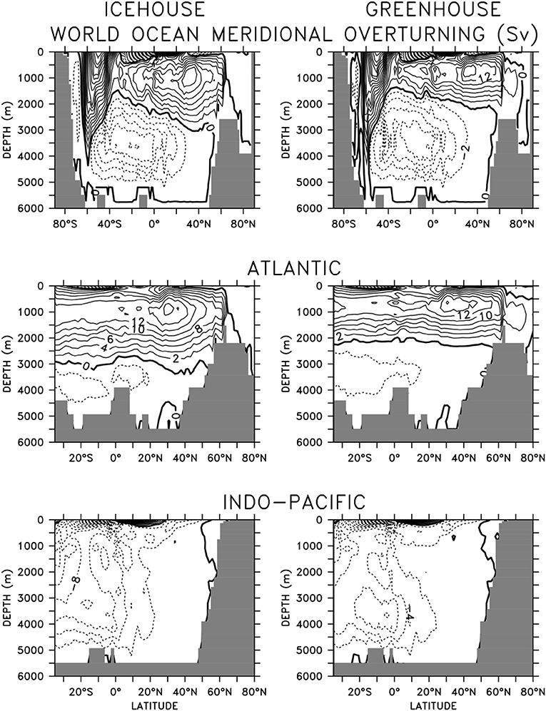
Figure 1. Basin-averaged meridional overturning in equilibrated (20,000 year integration) icehouse (left column) and greenhouse (right column) climates. Contours denote 2 Sv intervals.

Stronger AABW formation and shoaled AMOC affects water mass age (Figure 2). In the global mean, the deep southern hemisphere is younger by as much as 200 years in the greenhouse configuration, compared to the icehouse climate. The more vigorous anti-clockwise circulation is responsible for this difference. However, the more vigorous anti-clockwise circulation is also responsible for the aging of the deep northern hemisphere (also by as much as 200 years), as Southern Ocean-sourced deep water has a longer pathway into the northern hemisphere in a greenhouse climate, relative to the icehouse. Global average differences are dominated by the differences found in the deep North Atlantic, with the shoaled AMOC in the greenhouse climate and lengthened AABW pathway together contributing to an aging of as much as 600 years in the basin averaged profiles. These differences in circulation contribute to the substantial differences seen in ocean biogeochemistry described in the next section.

FIGURE 2

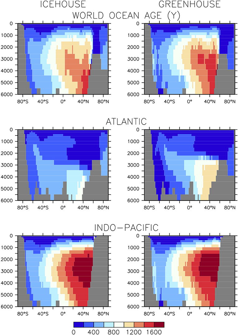
Figure 2. Basin-averaged water mass ideal age in equilibrated (20,000 year integration) icehouse (left column) and greenhouse (right column) climates.

3.1.2. Ocean Carbon and Biogeochemistry

The equilibrium and transient response of this model's icehouse and greenhouse carbon and biogeochemistry to prescribed atmospheric CO₂ forcing has been previously described (Kvale et al., 2018, 2019). As in Kvale K. F. et al. (2015b) and Kvale et al. (2019), net primary production (NPP) is greater in the warmer climate (enhanced by 28%, Table 1). Other production rates (e.g., calcification and nitrogen fixation) are also higher as both calcifiers and diazotrophs benefit from the more stratified conditions at the surface. However, not all rates of particle flux into the deep ocean are similarly enhanced. Particulate organic carbon (POC) flux at 130 m depth is 5% lower in the greenhouse climate despite higher NPP. This is because warmer seawater temperatures in the greenhouse climate accelerate nutrient recycling in the upper ocean, boosting production but also enhancing particle remineralization rates (Kvale K. F. et al., 2015b). Deep POC flux is unchanged from the icehouse climate because a greater proportion of the total POC flux is exported by calcite ballast, which protects the POC from water column remineralization. The effect on sedimentary carbonate deposition is large—a 24% higher CaCO₃:POC rain ratio at the top of the sediment in the greenhouse climate. However, the sediments themselves hold less carbonate in the greenhouse climate (Table 1) due to widespread calcite under-saturation in the deep ocean (Figure 3).

TABLE 1

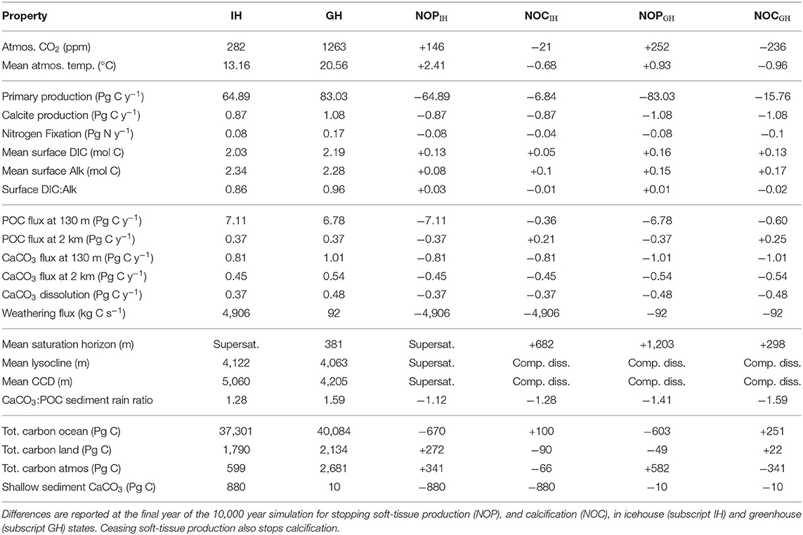
Table 1. Diagnosed global biogeochemical properties in icehouse (IH) and greenhouse (GH) climates, and change in these properties under Strangelove forcing.

FIGURE 3

Figure 3. Basin-averaged calcite saturation state in icehouse (left column) and greenhouse (right column) climates.

Carbonate base states are very different between simulated equilibrium icehouse and greenhouse oceans. The average depth of the greenhouse saturation horizon (where Ω_Ca = 1) is 381 m; shallower than in the nearly completely super-saturated icehouse ocean (Table 1). The sedimentary transition zone is also narrower; the greenhouse average lysocline (the depth where calcite dissolution in sediments is non-zero) is 59 m shallower than in the icehouse ocean, but the average CCD (defined in our model as where the rate of calcite dissolution meets or exceeds the rate of deposition in the sediments) is 855 m shallower (Table 1). The enhanced surface DIC:alkalinity ratio furthermore suggests an eroded buffer capacity in the greenhouse climate, relative to the icehouse state. An eroded ocean buffer capacity has been previously demonstrated for 2 and 3 times pre-industrial atmospheric CO₂ concentrations in a transient modern-ocean state (Egleston et al., 2010). The effect of this eroded buffer on carbon partitioning in our model is strong; the greenhouse climate has a smaller ratio between the ocean and atmosphere carbon pools (about 15 times more carbon in the ocean than in the atmosphere) than the icehouse climate (more than 62 times more carbon in the ocean). Calcite under-saturation occurs in the greenhouse ocean partly because the large amount of carbon introduced during the spin-up (resulting in 7% higher total carbon content in the ocean) increased the global DIC:alkalinity ratio). But also, the total ocean alkalinity inventory was kept constant as part of the method for spinning up the model greenhouse state. This prescribed constraint prevents carbonate compensation weathering feedback from restoring an icehouse DIC:alkalinity ratio in the greenhouse steady-state because it does not allow an increase in riverine weathering alkalinity flux into the oceans as a response to warming global temperatures. The implications of this constraint, and the resulting widespread under-saturation, are discussed in section 4.1.

3.2. Strangelove Simulations

We next describe the four idealized transient scenarios, two in which all soft-tissue production is stopped (which also stops calcification and predation, in icehouse and greenhouse climates) and two in which only calcite production is forced to stop (in icehouse and greenhouse climates). Atmospheric CO₂, climate, and ocean circulation are allowed to evolve freely for 10,000 years.

3.2.1. Atmospheric Carbon and Temperature Response

In the icehouse climate, stopping all soft-tissue production (which also stops calcification and predation) results in a rapid atmospheric CO₂ increase of 146 ppm (a 51% increase; Figure 4, left panel), due to the removal of the soft-tissue carbon and carbonate counter pumps and the concurrent response of the solubility pump. Stopping calcification (which also removes calcite ballasting of organic carbon) results in a CO₂ decrease of about 21 ppm (a 6.6% decrease). These sums are within the range of previous idealized studies (e.g., Sarmiento and Toggweiler, 1984; Volk and Hoffert, 1985; Marinov et al., 2008) and suggest calcification as having the lesser role in maintaining air-sea carbon gradients (and ballasting having a minor influence), with a relative strength calcifier of about one-sixth that of soft-tissue production (although, non-linear exchange between carbon pumps cannot be estimated by our experimental framework).

FIGURE 4

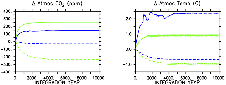
Figure 4. Atmospheric CO₂ response (left panel) in icehouse (blue lines) and greenhouse (green lines) to removing all soft-tissue production and calcification (solid lines) or calcification only (dashed lines). The concurrent response of globally averaged atmospheric temperature is shown in the (right panel).

In the greenhouse climate, removing all soft-tissue production and calcification produces an increase in atmospheric CO₂ of 252 ppm (a 20% increase). A larger absolute carbon increase in the atmosphere in a greenhouse climate is consistent with a reduced ocean buffer capacity with respect to the icehouse state. Differences in the response of the land carbon sink also contribute to the higher atmospheric CO₂ increase, and are described below.

The proportionally smaller atmospheric adjustment masks a relatively stronger response to ceased calcification (if additive pump effects are assumed). Stopping only calcification results in a CO₂ decrease of 236 ppm (a loss of 19% of the greenhouse equilibrated atmospheric concentration). The greenhouse ocean is uniquely positioned in terms of its surface DIC:alkalinity ratio, in that the average value is just <1. Seawater buffer factors are both at a minimum and roughly equally balanced when the DIC:alkalinity ratio is equal to 1 (Egleston et al., 2010), causing carbonate chemistry (and the solubility pump) to be strongly affected by small changes in alkalinity or DIC. Thus, while the major mechanisms of carbon drawdown due to the loss of calcifying phytoplankton are probably predominately thermodynamic, the overall impact on atmospheric CO₂ is stronger than in the icehouse climate. This demonstrates a relative strength of calcification in setting the atmospheric CO₂ concentration in the greenhouse climate to be about half that of soft-tissue production. The climate effect might be even stronger than demonstrated if the organic carbon ballasting by calcifiers is corrected for, but we do not consider this here.

Global mean atmospheric temperature adjusts to the change in atmospheric CO₂ in all simulations (Figure 4, right panel). The loss of both biologically-mediated pumps in the icehouse climate results in a warming of as much as 2.5°C, while in the greenhouse climate the warming stabilizes at about 0.9°C. This icehouse climate response (2.5/146=0.017°C per ppm) is about four times greater than compared to 0.004°C per ppm in the greenhouse climate (although, note these calculations do not adopt formal definitions of climate sensitivity). With the cessation of calcification, the icehouse climate response is about 0.032°C per ppm, while the greenhouse response is 0.004°C per ppm (and thus, showing no differences in sensitivity between stopping soft-tissue production and calcification and ceasing only calcification in the greenhouse climate state, but a roughly doubled sensitivity in the icehouse state to the loss of calcification only). A reduced transient climate response to CO₂ forcing and a reduced climate sensitivity in warmer climates has been documented for this model previously (Weaver et al., 2007), but what our results suggest is a reduced climate response to a weakened soft-tissue pump and carbonate counter-pump in a greenhouse state. Thus, while the total strength of calcification in setting the atmospheric CO₂ concentration relative to soft-tissue production is greater in the greenhouse climate and produces both a larger total and proportionately greater atmospheric CO₂ adjustment, and a larger total change in global temperature when it is stopped, the global climate response in both greenhouse simulations is weaker per addition of CO₂ to the atmosphere compared to in the icehouse state. As described in Weaver et al. (2007), the reason for this weaker response is due to model physical attributes, rather than carbon cycle differences. The primary factor is the logarithmic dependency of radiative forcing on CO₂ concentration (Myhre et al., 1998) that saturates at high atmospheric concentrations. Secondary factors include weakened radiative forcing feedbacks in the greenhouse climate. Cooler climates, such as our icehouse configuration, are more sensitive to albedo (von der Heydt et al., 2014) and convection feedbacks from sea ice (Weaver et al., 2007) and albedo feedback from vegetation (Meissner et al., 2003) that affect the absorption of short wave radiation (albedo) and the downward mixing of heat into the ocean (convection). Albedo feedbacks are weaker in the greenhouse climate because there is less sea ice and snow. These weakened feedbacks act in concert with the physio-chemical properties of CO₂ to stabilize our greenhouse climate, though we do not quantify the relative impacts here.

3.2.2. Global Carbon Cycle Response

The adjustment of carbon pools to the loss of ocean biological activity is very different in icehouse and greenhouse climates. By 5,000 years of integration, the icehouse atmospheric CO₂ concentration and inventory have stabilized at either 350 Pg C higher (in the case of ceased biological pumps) or 50 Pg C lower (in the case of ceased calcification) values (Figure 5). Interestingly, the loss of soft-tissue production and calcification causes a similar loss of carbon from the ocean in both greenhouse and icehouse climates (about 500 Pg C). However, in the icehouse climate that carbon moves in roughly equal proportion into the land and atmosphere partitions, whereas in the greenhouse climate the carbon goes into the atmosphere and is accompanied by an additional loss of carbon from the land reservoir of about 75 Pg C. A closer inspection of land carbon partitions (bottom row of Figure 5) reveals that the additional carbon entering the land model in the icehouse climate is taken up in roughly equal proportions by both the soil and vegetation. The additional atmospheric CO₂ fertilizes vegetation growth and enhances litter flux to the soil carbon pool in the warming climate. In the greenhouse climate, the loss of carbon from the land model is sourced mainly from the soil partition and is driven by temperature-dependent soil respiration, although a small (roughly 10 Pg C) amount of carbon is lost from the vegetation carbon pool, indicative of thermal stress.

FIGURE 5

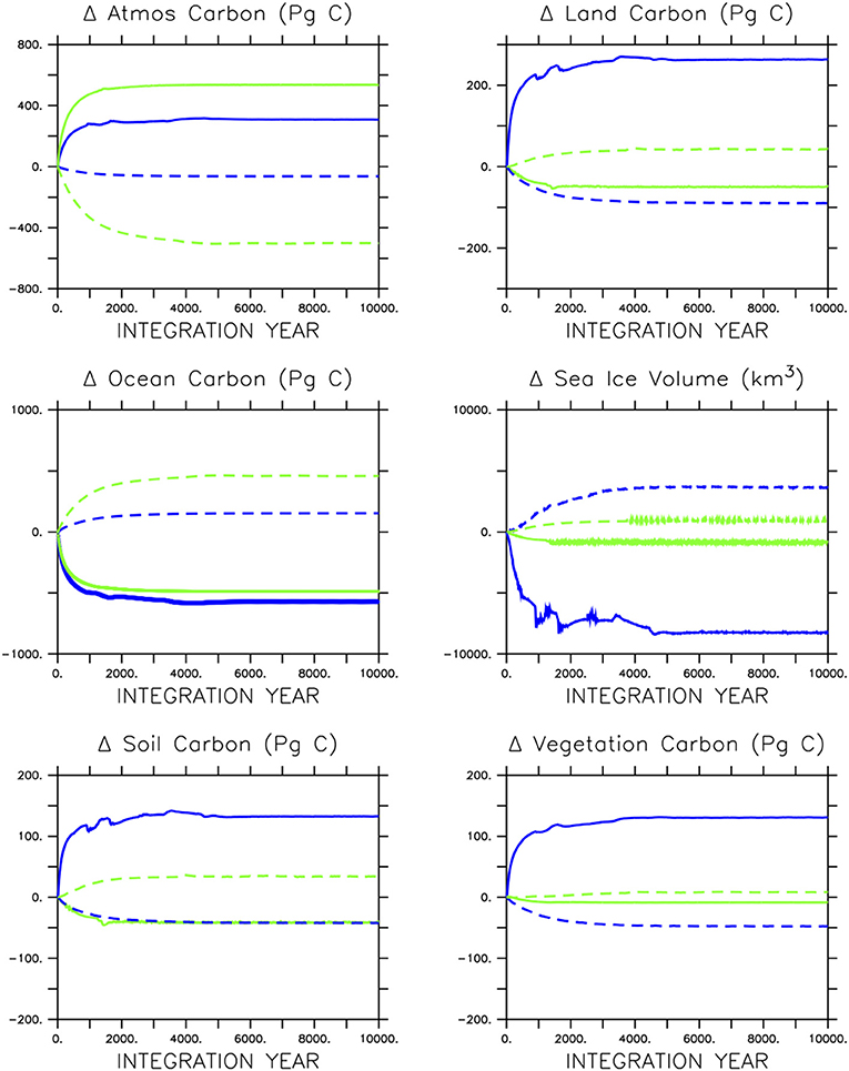
Figure 5. Response of carbon partitioning and sea ice volume in icehouse (blue lines) and greenhouse (green lines) climates to stopping soft-tissue production and calcification (solid lines) or calcification only (dashed lines).

In the icehouse climate, the loss of calcification produces a loss of about 100 Pg C from the land carbon model, with that carbon, as well as a small fraction of carbon from the atmosphere, ending up in the ocean. As with ceasing soft-tissue production, the loss of carbon from the land model is roughly equally proportioned between the soil and vegetation partitions. In the greenhouse climate, the loss of calcification moves a minor amount of carbon from the atmosphere onto the land (about 44 Pg C, due to cooling temperatures promoting soil storage) and a very large amount (about 500 Pg C) into the ocean. The loss of calcification deepens the saturation horizon by 298 m (greenhouse) and 682 m (icehouse) on global average (Table 1). The icehouse water column largely remains saturated, but the loss of CaCO₃ production and burial ceases sediment preservation. Carbonate sediments dissolve, producing a non-existent lysocline and CCD, as we define these terms. In the under-saturated greenhouse the water column remains under-saturated. Carbonate sediments dissolve with the loss of pelagic fluxes and both the lysocline and CCD are not recorded. Thus, a decoupling of saturation horizon (a water column property) and lysocline (a sediment property) occurs, with an increasingly saturated upper ocean and complete dissolution of the carbonate sediments.

4. Discussion

4.1. The Undersaturated Greenhouse Ocean Base State

Greenhouse oceans have been predicted to have equilibrium saturation states comparable to icehouse oceans over time periods longer than 10,000 years (Zeebe and Westbroek, 2003) due to the negative feedback of carbonate compensation, in which riverine weathering and sedimentary sources of alkalinity restore the water column DIC:alkalinity ratio. The process of carbonate compensation partially manifests in both the greenhouse spin-up terrestrial weathering (river) flux (which temporarily went negative, indicating an ocean sedimentary carbon release, then recovered to positive values after about 6,000 years; not shown) and in the shallow sediment carbon inventory (which also declined, stabilized, then started to increase at about 9,000 years). But the spin-up constraint of perfectly balanced weathering flux input and sedimentary burial flux never allows the net ocean alkalinity inventory to increase, which is the mechanism of fully restored carbonate saturation state. By the end of the 20,000 year greenhouse equilibration, the ocean has returned to being a net source of carbonate to the sediment model, despite a very stable and widespread calcite undersaturation in the deep ocean. This can be explained by rates of calcite export flux exceeding dissolution rates in the deep ocean and sediments. The sedimentary accumulation occurs because calcite production at the surface increases as a fixed proportion of organic detritus production by calcifiers (zooplankton and calcifying phytoplankton), which has increased due to warmer surface temperatures, and because even though calcite dissolution is thermodynamic, enough calcite still reaches the seafloor to be buried.

A possible means to restore deep ocean calcite saturation state in the greenhouse model back to icehouse buffer conditions would be to break the assumption of coupled weathering and carbonate burial fluxes, to allow additional alkalinity into the ocean system during the spin-up but without additional CaCO₃ burial (so weathering fluxes exceed benthic burial fluxes, restoring ${\text{CO}}_3^{2-}$ saturation). An ocean acidification impediment to biogenic calcification (Riebesell et al., 2000) to temporarily slow or stop pelagic carbonate production would accelerate carbonate saturation state restoration. Zeebe and Westbroek (2003) demonstrated a shortened neutralization time of roughly 1,000 years for fossil fuel release without calcification.

Another possible means to restore deep ocean calcite saturation state would be to limit the amount of atmospheric CO₂ that could enter the ocean over the spin-up by forcing it with a maximum amount of fossil fuel emissions, rather than prescribing an atmospheric concentration (which implicitly allows for unlimited fossil CO₂ emissions). In this framework, fossil CO₂ emissions would raise atmospheric CO₂ and warm and acidify the ocean but the total amount of carbon in the system would be limited. This would give the ocean sediments a chance to “catch-up” with the air/sea gas exchange. In the framework used, total carbon inventory (atmosphere/ocean/sediments/land) in the greenhouse steady-state is roughly 30% higher than estimates for these same pre-industrial partitions (Eby et al., 2009), plus all extractable fossil fuels (roughly 5,780 Pg C; Bauer et al., 2016).

Its unclear if either of these possible remedies would fully restore the UVic ESCM greenhouse ocean saturation state to icehouse conditions. There are two previous studies using an earlier version of the UVic ESCM (Pinsonneault et al., 2012; Zhang and Cao, 2016) that applied Ω_Ca dependencies to the calcification-production ratio to examine ocean responses to fossil carbon emissions. Both found large variations in ocean alkalinity over long (millennial) timescales, depending on parameterization, but none fully recovered the pre-industrial saturation state on the timescales simulated, and their simulations look like they would equilibrate to lower values if run longer. Eby et al. (2009) constrained emissions to “available” fossil carbon reserves and mentioned (but did not show) a recovery of surface pH on millennial timescales. However, none of these studies discussed the potential implications of their weathering flux parameterization (all held fluxes constant at pre-industrial rates), so its unclear how much the weathering fluxes might have contributed to their results. Meissner et al. (2012) tested weathering flux parameterizations and how they might influence carbonate saturation state recovery, but without ocean acidification-driven changes to calcification. They also found a strong dependency in saturation state recovery on parameterization, none of which fully recovered over their 12,000 year simulations. In their figures it appears the ocean saturation state will equilibrate to something less than their pre-industrial (despite limited CO₂ emissions scenarios and sedimentary carbonate compensation), so it appears likely that both weathering and calcification parameterizations will need to be adjusted in our model to produce a fully compensated greenhouse ocean. However, even box modeling suggests sedimentary carbonate compensation cannot fully neutralize large (5,000 Pg C) emissions on hundred-thousand year timescales (Zachos et al., 2008). Million-year timescales are more representative of a “full” restoration of initial state (Coxall et al., 2006; Zeebe, 2012).

But how realistic is a fully compensated, highly saturated greenhouse ocean? Zeebe and Westbroek (2003) demonstrate that in a Cretan ocean (both our greenhouse and icehouse steady-states fit within this category) it is possible to maintain widespread undersaturation and a shallow CCD with high rates of biogenic pelagic calcification, if the weathering flux is sufficiently low. So, despite certain aspects of our model (unlimited atmospheric CO₂, pelagic calcification insensitive to ocean acidification, and a fixed weathering flux diagnosed over equilibration) being unrealistic, its ocean carbon cycle characteristics are physically possible under the right real-world circumstances. Note also, that Zeebe and Westbroek (2003) considered a 1 km change in the CCD to be small, therefore our initial depressed greenhouse saturation state is not inconsistent with their idealized Cretan carbon chemistry. If our model were to produce a geologic record over the greenhouse spin-up, it would show a millennial carbonate sediment erosional event followed by a stabilization of high calcification and ongoing coastal/shelf carbonate sediment deposition. The shoaling of the CCD (diagnosed by mapping where sedimentary dissolution rates exceed sedimentary deposition rates) by about 800 meters is accompanied by an atmospheric CO₂ increase of about 1,000 ppm relative to the icehouse state. The magnitude of such a change is consistent with the 1–1.5 km deepening reported for the Pacific CCD and thousands of ppm decline in atmospheric CO₂ over the Cenozoic, as well as shorter (100,000 year) excursions of the CCD of between 0.5 and 1 km depth (Pälike et al., 2012). The shallower remineralization depth and enhanced carbonate production are also consistent with δ13C reconstructions of the Eocene (early Cenozoic, John et al., 2013). There may have been periods in the more distant past with greenhouse-level CO₂ concentrations and a similar or stronger ocean carbon buffer than found in the modern ocean (due to multi-million year adjustment of silicate weathering, e.g., Zachos et al., 2008; Zeebe, 2012). But note also that paleo-records of the CCD record sedimentary processes, not the whole water-column. Previous modeling has demonstrated the CCD (as a sediment property integral of a range of fluxes) is well-buffered over both short and long-term perturbations which can cause CCD and atmospheric CO₂ trends to be decoupled (Pälike et al., 2012).

4.2. Relative Stability of Carbon and Climate

The transient simulations described above reveal very different carbon cycle and climate responses to the loss of ocean biological activity in icehouse and greenhouse climate states. By virtue of a relatively enhanced ocean buffering capacity and cooler temperatures, the icehouse state has a relatively stable atmospheric carbon inventory that allows the ocean solubility pump and land carbon partition to mitigate changes due to the loss of either ocean soft-tissue production or calcification. However, also by virtue of cooler temperatures (and lower atmospheric CO₂ concentrations), the icehouse state has a relatively less stable climate, with a temperature response to changing atmospheric CO₂ about four times greater than the greenhouse state. This greater sensitivity is due to fundamental properties of CO₂ as well as radiative forcing feedbacks from both the land and sea ice albedo in our model that are reduced in the greenhouse climate. These factors contribute to an enhanced radiative forcing “buffer” in the greenhouse climate, increasing climate stability despite the highly unstable and eroded ocean carbon buffer.

The Pälike et al. (2012) Pacific CCD reconstruction reveals that greenhouse (1,000-ppm CO₂) periods prior to the EOT are accompanied by decreased stability of, and a shallower, CCD (their Figure 2, prior to about 34 Ma) whereas more modern icehouse (hundred-ppm) CO₂ levels show a roughly 15 My period of strong CCD stability, at a deeper depth level. This overall CCD deepening and stabilization was attributed to a shift to a greater proportion of pelagic calcification relative to shelf calcification (Pälike et al., 2012), which would also be consistent with the box model tests of Zeebe and Westbroek (2003). But they tested this hypothesis in their more complex earth system model (GENIE) and found it was insufficient to move the CCD as far as observations suggest (Pälike et al., 2012). However, in our model the CCD does move to the right order (between equilibrium states), and our transient simulations suggest a very simple mechanism for icehouse carbon cycle stabilization (enhanced chemical buffer). An increased “predictability” in the Westerhold et al. (2020) hothouse/warmhouse climate states relative to coolhouse/icehouse climate states, might furthermore be consistent with our observation of a greenhouse climate less sensitive to changes in CO₂ and an icehouse climate dominated more by ice albedo feedbacks and the non-linear CO₂ radiative forcing sensitivity.

That relative climate (temperature) stability is greater in the greenhouse state, despite a less stable carbon cycle, might at least partly explain the apparent selective extinction both of marine organisms in general and of calcifying organisms specifically, as well as calcifiers' recovery lag after climate perturbation (Veron, 2008). Greenhouse climates experience intermittent calcification crises (Kidder and Worsley, 2010), which makes sense given the precarious buffer conditions a high DIC:alkalinity ratio might produce. At the same time, coral reef gaps- extended periods of absence in the rock record of coral reefs- appear to coincide with rapidly dropping atmospheric CO₂ in several instances (the late Devonian, early Jurassic, and early Cenozoic; Veron, 2008 their Figure 3). Thus, while an external perturbation (e.g., substantial volcanic activity), might temporarily shut down calcification in a greenhouse state (and do so more readily than in an icehouse climate), its loss could provide a powerful negative feedback on atmospheric CO₂, hastening the return of the initial state. Such a powerful negative feedback on atmospheric CO₂ was also noted by Zeebe and Westbroek (2003).

Our results are also interesting in light of Eichenseer et al. (2019), who calculated an increasing “biotic” control on the ecological success of aragonite calcifiers since the Paleozoic. In their conceptual model, which they derived from analysis of species indices, the rise of pelagic calcification increasingly buffered ocean chemistry (consistent with the results of Zeebe and Westbroek, 2003), which in turn allowed the proliferation of calcifier species after the middle Jurassic. Thus, calcification became increasingly self-perpetuating and less reliant on environmental “abiotic” control. The periods they examined were largely in a greenhouse state, but their Figure 1a shows what appears to be a state change around the Oligocene back to what might be considered a more abiotically controlled paradigm (although their statistical analysis was inconclusive for this time period). This analysis of a more biotic control on calcifiers' success in a greenhouse state due to chemical buffer stabilization can be flipped to also state that the calcifiers' ecological success in a greenhouse state can exert a relatively greater impact on environmental conditions (and perhaps, climate), which is consistent with our results using an entirely independent methodology.

In our greenhouse model spin-up we did not consider ocean acidification effects on calcification (Riebesell et al., 2000). If we had, over the greenhouse spin-up calcification would have slowed or ceased temporarily, which would have allowed the sediments to more quickly neutralize the atmospheric CO₂ intrusion (Zeebe and Westbroek, 2003). Calcification would have restarted when Ω_Ca was sufficiently restored and the equilibrated greenhouse ocean might have a similar buffer capacity as the icehouse ocean. This enhanced buffer might therefore “prime” the ocean to accept a far larger quantity of atmospheric CO₂ with the stoppage of calcification than what we simulate. This arrangement might be more representative of a high calcification, high Ω_Ca greenhouse ocean such as that of the Cretaceous (Zeebe, 2012). However, if in our model simulations we considered an e.g. halved calcification rate for the greenhouse steady-state with a low Ω_Ca saturation state, we would expect a somewhat larger CO₂ increase with ceased soft tissue production and calcification, and a somewhat smaller CO₂ decrease with ceased calcification only. Such a parameterization is arguably inappropriate for model spin-up, given the geological record reveals a positive relationship between atmospheric CO₂ and calcification, with enhanced calcification during high-CO₂ intervals (Bolton et al., 2016) despite a shallower CCD.

Our model results suggest an enhanced role of calcifying phytoplankton in regulating atmospheric CO₂ in greenhouse climates, but we cannot quantify that role precisely because we do not apply separation techniques to the carbon cycle (e.g., Koeve et al., 2014) and also include carbon exchange with a land model. The strongly reduced buffering capacity of the greenhouse ocean (demonstrated as widespread calcite undersaturation) suggests response of atmospheric CO₂ to the loss of biological pumps is enhanced by the solubility pump in this state. Quantification of the absolute strengths of these three carbon pumps requires implementing both carbon separation as well as removing the land model, and would be an interesting exercise in light of our results. Furthermore, a quantitative description of the interactive and changing seawater buffer factors with long-timescale carbonate compensation feedback, in parallel with a sensitivity study of weathering flux and ocean acidification parameterizations, would be another very interesting future exercise.

Data Availability Statement

The datasets generated for this study can be found in the GEOMAR OPenDAP repository at https://data.geomar.de/thredds/20.500.12085/ab647f7e-042f-461d-b6dc-6c97d1b8325f/catalog.html.

Author Contributions

KK wrote the manuscript, with input and editing by WK and NM. KK and WK designed and KK ran the simulations. All authors contributed to the article and approved the submitted version.

Funding

Funding for this study was provided by GEOMAR Helmholtz Centre for Ocean Research, Kiel. NM acknowledges funding from the Helmholtz-Climate-Initiative (HI-CAM), which is funded by the Helmholtz Associations Initiative and Networking Fund.

Conflict of Interest

The authors declare that the research was conducted in the absence of any commercial or financial relationships that could be construed as a potential conflict of interest.

Acknowledgments

The authors acknowledge computer resources provided by Kiel University and GEOMAR.

References

Archer, D. (1996). A data-driven model of the global calcite lysocline. Glob. Biogeochem. Cycles 10, 511–526. doi: 10.1029/96GB01521

CrossRef Full Text | Google Scholar

Bauer, N., Mouratiadou, I., Luderer, G., Baumstark, L., Brecha, R. J., Edenhofer, O., et al. (2016). Global fossil energy markets and climate change mitigation -an analysis with remind. Clim. Change 136, 69–82. doi: 10.1007/s10584-013-0901-6

CrossRef Full Text | Google Scholar

Berner, R. A. (1990). Atmospheric carbon dioxide levels over phanerozoic time. Science 249:4975. doi: 10.1126/science.249.4975.1382

PubMed Abstract | CrossRef Full Text | Google Scholar

Berner, R. A. (1994). GEOCARB II: A revised model of atmospheric co2 over phanerozoic time. Am. J. Sci. 294:1. doi: 10.2475/ajs.294.1.56

CrossRef Full Text | Google Scholar

Berner, R. A., and Canfield, D. E. (1989). A new model for atmospheric oxygen over phanerozoic time. Am. J. Sci. 289, 333–361. doi: 10.2475/ajs.289.4.333

PubMed Abstract | CrossRef Full Text | Google Scholar

Bolton, C. T., Hernandez-Sanchez, M. T., Fuertes, M.-A., Gonzalez-Lemos, S., Abrevaya, L., Mendez-Vicente, A., et al. (2016). Decrease in coccolithophore calcification and CO2 since the middle Miocene. Nat. Commun. 7:10284. doi: 10.1038/ncomms10284

PubMed Abstract | CrossRef Full Text | Google Scholar

Coxall, H. K., D'Hondt, S., and Zachos, J. C. (2006). Pelagic evolution and environmental recovery after the Cretaceous-Paleogene mass extinction. Geology 34, 297–300. doi: 10.1130/G21702.1

CrossRef Full Text | Google Scholar

Earth System Research Laboratories, G. M. L. (2020). Trends in Atmospheric Carbon Dioxide.

Google Scholar

Eby, M., Zickfeld, K., Montenegro, A., Archer, D., Meissner, K. J., and Weaver, A. J. (2009). Lifetime of anthropogenic climate change: millennial time scales of potential CO2 and surface temperature perturbations. J. Clim. 22, 2501–2511. doi: 10.1175/2008JCLI2554.1

CrossRef Full Text | Google Scholar

Egleston, E. S., Sabine, C. L., and Morel, F. M. M. (2010). Revelle revisited: Buffer factors that quantify the response of ocean chemistry to changes in DIC and alkalinity. Glob. Biogeochem. Cycles 24. doi: 10.1029/2008GB003407

CrossRef Full Text | Google Scholar

Eichenseer, K., Balthasar, U., Smart, C. W., Stander, J., Haaga, K. A., and Kiessling, W. (2019). Jurassic shift from abiotic to biotic control on marine ecological success. Nat. Geosci. 12, 638–642. doi: 10.1038/s41561-019-0392-9

CrossRef Full Text | Google Scholar

Garcia, H. E., Locarnini, R., Boyer, T., Antonov, J., Zweng, M., Baranova, O., and Johnson, D. (2009). World Ocean Atlas 2009: Nutrients (Phosphate, Nitrate, Silicate). Number NOAA Atlas NESDIS 71. U.S. Government Printing Office, Washington, DC.

Google Scholar

Huber, M., and Caballero, R. (2011). The early Eocene equable climate problem revisited. Clim. Past 7, 603–633. doi: 10.5194/cp-7-603-2011

PubMed Abstract | CrossRef Full Text | Google Scholar

John, E. H., Pearson, P. N., Coxall, H. K., Birch, H., Wade, B. S., and Foster, G. L. (2013). Warm ocean processes and carbon cycling in the Eocene. Philos. Trans. R. Soc. A Math. Phys. Eng. Sci. 371:2001. doi: 10.1098/rsta.2013.0099

PubMed Abstract | CrossRef Full Text | Google Scholar

John, E. H., Wilson, J. D., Pearson, P. N., and Ridgwell, A. (2014). Temperature-dependent remineralization and carbon cycling in the warm Eocene oceans. Palaeogeogr. Palaeoclimatol. Palaeoecol. 413, 158–166. doi: 10.1016/j.palaeo.2014.05.019

PubMed Abstract | CrossRef Full Text | Google Scholar

Key, R., Kozyr, A., Sabine, C., Lee, K., Wanninkhof, R., Bullister, J., et al. (2004). A global ocean carbon climatology: results from GLODAP. Glob. Biogeochem. Cycles 18, 1–23. doi: 10.1029/2004GB002247

CrossRef Full Text | Google Scholar

Kidder, D. L., and Worsley, T. R. (2010). Phanerozoic large igneous provinces (LIPs), HEATT (haline euxinic acidic thermal transgression) episodes, and mass extinctions. Palaeogeogr. Palaeoclimatol. Palaeoecol. 295, 162–191. doi: 10.1016/j.palaeo.2010.05.036

CrossRef Full Text | Google Scholar

Koeve, W., Duteil, O., Oschlies, A., Kähler, P., and Segschneider, J. (2014). Methods to evaluate caco₃ cycle modules in coupled global biogeochemical ocean models. Geosci. Model Dev. 7, 2393–2408. doi: 10.5194/gmd-7-2393-2014

CrossRef Full Text | Google Scholar

Koeve, W., Wagner, H., Kähler, P., and Oschlies, A. (2015). 14C-age tracers in global ocean circulation models. Geosci. Model Dev. 8, 2079–2094. doi: 10.5194/gmd-8-2079-2015

CrossRef Full Text | Google Scholar

Kvale, K., Meissner, K., Keller, D., Schmittner, A., and Eby, M. (2015a). Explicit planktic calcifiers in the University of Victoria Earth System Climate Model, version 2.9. Atmos. Ocean 1–19. doi: 10.1080/07055900.2015.1049112

CrossRef Full Text | Google Scholar

Kvale, K., Turner, K. E., Keller, D. P., and Meissner, K. J. (2018). Asymmetric dynamical ocean responses in warming icehouse and cooling greenhouse climates. Environ. Res. Lett. 13:125011. doi: 10.1088/1748-9326/aaedc3

CrossRef Full Text | Google Scholar

Kvale, K. F., Meissner, K. J., and Keller, D. P. (2015b). Potential increasing dominance of heterotrophy in the global ocean. Environ. Res. Lett. 10, 37–41. doi: 10.1088/1748-9326/10/7/074009

CrossRef Full Text | Google Scholar

Kvale, K. F., Turner, K., Landolfi, A., and Meissner, K. J. (2019). Phytoplankton calcifiers control nitrate cycling and the pace of transition in warming icehouse and cooling greenhouse climates. Biogeosciences 16, 1019–1034. doi: 10.5194/bg-16-1019-2019

CrossRef Full Text | Google Scholar

Marinov, I., Gnanadesikan, A., Sarmiento, J. L., Toggweiler, J. R., Follows, M., and Mignone, B. K. (2008). Impact of oceanic circulation on biological carbon storage in the ocean and atmospheric pco2. Glob. Biogeochem. Cycles 22, 1–15. doi: 10.1029/2007GB002958

CrossRef Full Text | Google Scholar

McKenzie, N. R., and Jiang, H. (2019). Earth's outgassing and climatic transitions: the slow burn towards environmental “catastrophes?” Elements 15, 325–330. doi: 10.2138/gselements.15.5.325

CrossRef Full Text | Google Scholar

Meissner, K., Weaver, A., Matthews, H., and Cox, P. (2003). The role of land surface dynamics in glacial inception: a study with the UVic Earth System Model. Clim. Dyn. 21, 515–537. doi: 10.1007/s00382-003-0352-2

CrossRef Full Text | Google Scholar

Meissner, K. J., McNeil, B. I., Eby, M., and Wiebe, E. C. (2012). The importance of the terrestrial weathering feedback for multimillennial coral reef habitat recovery. Glob. Biogeochem. Cycles 26, 1–20. doi: 10.1029/2011GB004098

CrossRef Full Text | Google Scholar

Members, P. P. (2013). Making sense of palaeoclimate sensitivity. Nature. 491, 683–691.

PubMed Abstract | Google Scholar

Myhre, G., Highwood, E. J., Shine, K. P., and Stordal, F. (1998). New estimates of radiative forcing due to well mixed greenhouse gases. Geophys. Res. Lett. 25, 2715–2718. doi: 10.1029/98GL01908

CrossRef Full Text | Google Scholar

Pälike, H., Lyle, M. W., Nishi, H., Raffi, I., Ridgwell, A., Gamage, K., et al. (2012). A cenozoic record of the equatorial pacific carbonate compensation depth. Nature 488, 609–614. doi: 10.1038/nature11360

PubMed Abstract | CrossRef Full Text | Google Scholar

Pinsonneault, A. J., Matthews, H. D., Galbraith, E. D., and Schmittner, A. (2012). Calcium carbonate production response to future ocean warming and acidification. Biogeosciences 9, 2351–2364. doi: 10.5194/bg-9-2351-2012

CrossRef Full Text | Google Scholar

Riebesell, U., Zondervan, I., Rost, B., Tortell, P. D., Zeebe, R. E., and Morel, F. M. M. (2000). Reduced calcification of marine plankton in response to increased atmospheric co2. Nature 407, 364–367. doi: 10.1038/35030078

PubMed Abstract | CrossRef Full Text | Google Scholar

Sarmiento, J. L., and Toggweiler, J. R. (1984). A new model for the role of the oceans in determining atmospheric P CO2. Nature 308, 621–624. doi: 10.1038/308621a0

CrossRef Full Text | Google Scholar

Schmittner, A., Oschlies, A., Matthews, H. D., and Galbraith, E. D. (2008). Future changes in climate, ocean circulation, ecosystems, and biogeochemical cycling simulated for a business-as-usual CO2 emission scenario until year 4000 AD. Glob. Biogeochem. Cycles 22, 1–21. doi: 10.1029/2007GB002953

CrossRef Full Text | Google Scholar

Tyrrell, T. (1999). The relative influences of nitrogen and phosphorus on oceanic primary production. Nature 400, 525–531. doi: 10.1038/22941

CrossRef Full Text | Google Scholar

Veron, J. E. N. (2008). Mass extinctions and ocean acidification: biological constraints on geological dilemmas. Coral Reefs 27, 459–472. doi: 10.1007/s00338-008-0381-8

CrossRef Full Text | Google Scholar

Volk, T., and Hoffert, M. (1985). Ocean carbon pumps: analysis of relative strengths and efficiencies in ocean-driven atmospheric CO2 changes. Am. Geophys. Union 32, 99–110. doi: 10.1029/GM032p0099

CrossRef Full Text | Google Scholar

von der Heydt, A. S., Köhler, P., van de Wal, R. S. W., and Dijkstra, H. A. (2014). On the state dependency of fast feedback processes in (paleo) climate sensitivity. Geophys. Res. Lett. 41, 6484–6492. doi: 10.1002/2014GL061121

CrossRef Full Text | Google Scholar

Weaver, A., Eby, M., Wiebe, E., Bitz, C., Duffy, P., Ewen, T., et al. (2001). The UVic Earth System Climate Model: Model description, climatology, and applications to past, present and future climates. Atmosphere 39, 361–428. doi: 10.1080/07055900.2001.9649686

CrossRef Full Text | Google Scholar

Weaver, A. J., Eby, M., Kienast, M., and Saenko, O. A. (2007). Response of the Atlantic meridional overturning circulation to increasing atmospheric CO2: Sensitivity to mean climate state. Geophys. Res. Lett. 34, 1–5. doi: 10.1029/2006GL028756

CrossRef Full Text | Google Scholar

Westerhold, T., Marwan, N., Drury, A. J., Liebrand, D., Agnini, C., Anagnostou, E., et al. (2020). An astronomically dated record of earth' climate and its predictability over the last 66 million years. Science 369, 1383–1387. doi: 10.1126/science.aba6853

PubMed Abstract | CrossRef Full Text | Google Scholar

Zachos, J., Pagani, M., Sloan, L., Thomas, E., and Billups, K. (2001). Trends, rhythms, and aberrations in global climate 65 ma to present. Science 292, 686–693. doi: 10.1126/science.1059412

PubMed Abstract | CrossRef Full Text | Google Scholar

Zachos, J. C., Dickens, G. R., and Zeebe, R. E. (2008). An early Cenozoic perspective on greenhouse warming and carbon-cycle dynamics. Nature 451, 279–283. doi: 10.1038/nature06588

PubMed Abstract | CrossRef Full Text | Google Scholar

Zeebe, R. E. (2012). History of seawater carbonate chemistry, atmospheric co2, and ocean acidification. Annu. Rev. Earth Planet. Sci. 40, 141–165. doi: 10.1146/annurev-earth-042711-105521

CrossRef Full Text | Google Scholar

Zeebe, R. E., and Westbroek, P. (2003). A simple model for the caco3 saturation state of the ocean: the “strangelove,” the “neritan,” and the “cretan” ocean. Geochem. Geophys. Geosyst. 4, 1–26. doi: 10.1029/2003GC000538

CrossRef Full Text | Google Scholar

Zhang, H., and Cao, L. (2016). Simulated effect of calcification feedback on atmospheric co2 and ocean acidification. Sci. Rep. 6:20284. doi: 10.1038/srep20284

PubMed Abstract | CrossRef Full Text | Google Scholar