A Multi-Sensor and Modeling Approach for Mapping Light Under Sea Ice During the Ice-Growth Season

Introduction

The Arctic is undergoing a period of profound transformation in response to anthropogenic warming, with the loss of the sea ice cover one of its starkest changes. Since the late 1970s, the summer ice cover has shrunk in area by 40%, whereas changes in winter have been much smaller, on the order of 10%. This loss in sea ice area has been accompanied by loss of the thick multiyear sea ice, which today makes up only 30% of the Arctic Ocean sea ice compared to 70% 40 years ago (Maslanik et al., 2011; Stroeve and Notz, 2018). These changes reflect thinning of the ice cover, which has thinned over the central Arctic basin by 65% since 1975 (Lindsay and Schweiger, 2015). While the 2012 sea ice extent minimum was striking, variability is increasing, in relation to a thinning ice cover (Goosse et al., 2009) and recent departures from average conditions during the transition seasons have become even more anomalous than in summer: Arctic sea ice extent (defined as the area with at least 15% sea ice concentration, SIC) in May and November 2016 fell nearly 4 standard deviations below the 1981–2010 long-term average (Stroeve and Notz, 2018). This represents a distinct change in the seasonality of the Arctic Ocean as the melt onset is happening earlier and the fall freeze-up later (Stroeve et al., 2014; Stroeve and Notz, 2018; Lebrun, 2019).

Shortwave radiation, and its visible fraction in particular, provides an essential control on the Arctic surface energy budget (Maykut, 1986; Perovich et al., 2007) and on microbial ecosystems (Wassmann and Reigstad, 2011). In addition, light transmitted under sea ice warms the upper ocean and in turn drives basal sea ice melt (e.g., Maykut and McPhee, 1995; Vivier et al., 2016).

In regards to ecosystems, light is the main energy source for the development of phytoplankton and sea ice algae. Together sea ice algae and phytoplankton form the base of the Arctic marine food web, sustaining directly sea ice associated macrofaunal and pelagic zooplankton (Kohlbach et al., 2016, 2017). The sea ice scape greatly affects the amount of light reaching the upper ocean. Sea ice and especially its snow cover are excellent reflectors, whereas melt ponds and open water within the pack effectively act as windows, increasing light supply to the surface ocean (Frey et al., 2011; Assmy et al., 2017). In turn, sea ice drastically attenuates light reaching the ocean surface, which would reduce the depth over which waters are biologically productive (Sverdrup, 1953; Horvat et al., 2017). On the other hand, the ice underside provides a highly variable and heterogeneous habitat for different ice-associated macrofaunal as well as certain zooplankton whose vertical migration is often triggered by food availability and periodic changes in light availability (e.g., Berge et al., 2014).

As the winter ends and the sun returns above the horizon again, light is the major factor controlling algal growth onset (Castellani et al., 2017) and production (Horner and Schrader, 1982). Ice algae are able to take advantage of low under-ice photosynthetic active radiation (PAR) levels during this time of year (Mock and Gradinger, 1999) at sites with a relatively low snow depth cover. Snow distribution in spring (March–April–May) is thus the major physical driver of ice algae phenology, and changes in sea ice and snow scape are expected to affect both phytoplankton and ice algal activity. The clearest example is provided by earlier ice retreat and delays in freeze-up, which have cascading impacts on light availability. For one, earlier melt onset allows light to enter the Arctic Ocean earlier and closer to the summer solstice than it used to, whereas delays in freeze-up have extended the light season into early winter, leading to visible Arctic planktonic activity earlier in spring and later into fall (Arrigo and van Dijken, 2011; Ardyna et al., 2014). The extended open water season not only increases the coupling between the ocean and the atmosphere, but additionally reduces the amount of time over which snow can accumulate on the sea ice (Webster et al., 2014; Stroeve et al., 2020). Other expected changes in sea ice scape, such as melt pond fraction and depth, currently challenging to detect (Zhang et al., 2018), would also influence marine autotrophs in polar seas in summer. Together these changes have important implications for the in-ice and under-ice biota, influencing light availability, ocean properties, and the timing of sea ice algae and phytoplankton blooms (Bluhm et al., 2017). These changes in sea ice scape are also accompanied by stratification and circulation changes, which also affect under-ice plankton activity, via the modulation of nutrient fluxes, critical to the total possible photosynthesis over the year (Vancoppenolle et al., 2013; Randelhoff et al., 2020). In other words, changes in the sea ice and snow characteristics alters phenology of primary productivity in the Arctic Ocean.

However, our understanding of how this sea ice changes impact primary productivity is still in its infancy. Our understanding of ecosystem function, sea ice, and upper ocean processes in the Arctic Ocean has been mostly derived from a multiyear ice setting, rather than the thinner first-year ice dominated Arctic of recent years. As a result, our current climate models use formulations of light transmission through sea ice in large part based on parameterizations for multiyear sea ice (e.g., Grenfell and Maykut, 1977; Fichefet and Morales Maqueda, 1997; Perovich et al., 2002; Briegleb and Light, 2007). Recent observations have shown that the transition from a multiyear to first-year ice-dominated Arctic Ocean has increased the amount of light reaching the upper ocean, with a threefold increase in light transmittance (Nicolaus et al., 2012). This was primarily a result from increased melt pond fraction over first-year sea ice compared to multiyear ice. Nicolaus et al. (2012) also found that energy absorption in first-year ice was 50% larger.

Quantifying the availability of light under the ice is key if we are to better understand how primary productivity functions in today’s Arctic, and how it may change in the future. Specifically, we need to better quantify the availability of PAR (400–700 nm) under the ice, and how this affects ecosystem function. This requires improved parameterizations of the light climate under an Arctic Ocean dominated by first-year sea ice with reduced winter snow cover and increased melt pond fraction in summer. The most comprehensive set of measurements from six years of in situ observations from spring to autumn were recently published by Katlein et al. (2019). These data, while still somewhat limited in both space and time, are improving our ability to derive robust relationships between ice conditions (e.g., thickness, melt pond fraction, snow depth) and light transmission.

To scale up to the pan-Arctic level, we must rely on satellite observations and model-produced data sets of the key system controls. Satellites provide several sea ice variables needed to quantify under-ice light, including (a) surface albedo, (b) melt pond fraction, (c) timing of melt onset, (d) SIC, (e) sea ice thickness (SIT), and (f) surface topography. A key limitation has been the snow depth on sea ice, which has generally been poorly mapped with satellites. This is particularly important before the melt season starts because snow depth plays a larger role than ice thickness in limiting light availability under the ice (e.g., Mundy et al., 2005). Nevertheless, several recent advances in modeling snow accumulation over sea ice have been made, using a combination of modeling with atmospheric reanalyses and satellite drift datasets (e.g., Blanchard-Wrigglesworth et al., 2018; Petty et al., 2018; Liston et al., 2020), as well as combining dual radar frequencies from satellite altimeters (e.g., Lawrence et al., 2018).

Another key limitation is the lack of ice thickness information in summer, as well as the temporal and spatial coverage during winter. Prior to the launch of ICESat-2, pan-Arctic SIT has mostly been monitored using satellite radar altimeter missions that span 1993 through present. These have been obtained at various temporal and spatial resolutions, but are entirely limited to the cold (non-melt) season (i.e., October through April). Since 2010, CryoSat-2 has provided monthly pan-Arctic SIT estimates (e.g., Laxon et al., 2013; Tilling et al., 2018). With the launch of ICESat-2 in September 2018, SIT may potentially also be retrieved in summer. Further, the combination of ICESat-2 and CryoSat-2 freeboards may give a direct estimate of snow depth (Kwok and Markus, 2018), but this strongly depends on the location of the dominant scattering horizon of CryoSat-2, which is unlikely to be from the snow/ice interface (e.g., Willatt et al., 2011). Other important sea ice features for quantifying light availability under the ice include (1) melt ponds, (2) ridges, and (3) leads. Each of these have been mapped using satellites with either limited success in the case of melt ponds (Tschudi et al., 2008; Rösel and Kaleschke, 2012; Scharien et al., 2017; Yackel et al., 2018), or not mapped over large spatial and long temporal scales in the case of leads (e.g., Eicken et al., 2006; Zakharova et al., 2015; Willmes and Heinemann, 2016; Lewis and Hutchings, 2019), and while surface roughness has been detected (e.g., Landy et al., 2015; Petty et al., 2016; Nolin and Mar, 2019), ridge height has yet to be retrieved from satellites. Nevertheless, ridged ice can be important biological hotspots (e.g., Fernández-Méndez et al., 2018).

Given that current uncertainties in the light limitation level (Popova et al., 2010), as well as nutrient uncertainties undermine confidence in primary production for the 21st century (Vancoppenolle et al., 2013), progress is needed on all fronts. This paper focuses on our capabilities for mapping light between 400 and 700 nm under ice with currently available satellite-derived products and state-of-the art light parameterizations, and suggests ways forward to fill important gaps to improve our understanding on how light transmission is changing in a changing sea ice environment. Given the limitations with today’s satellite products on a pan-Arctic scale, we are presently restricted to monthly means over the October to April time-period. Because of these inherent difficulties, we focus here on the CryoSat-2 time period (October to April, 2010 to 2018), and examine how accurately we can estimate under-ice light fields in a relevant manner for physical and ecosystem studies at the pan-Arctic scale. Prior to the melt season, snow depth will play the dominant role in limiting light entering the upper ocean (e.g., Katlein et al., 2019), and thus the focus is largely on how snow variability and change impact under-ice light levels. We further extend our time-period to May and July to examine how snow depth trends impact light transmission through snow as the snowpack begins to melt.

Methodology and Approach

Solar Transmission Calculations

To map the under-ice light with the satellite products, we rely on a generalization of the approach proposed by Maykut and Untersteiner (1971) and Grenfell and Maykut (1977), based on a specification of apparent optical properties (AOPs), namely surface albedo (α) and vertical attenuation coefficients (κ), assuming a two-level Beer–Lambert exponential decay in the snow-ice system. This approach considers that the snow-ice system is comprised of two layers, which absorb most of the radiation, the so-called single scattering layer (SSL), and a lower layer, where, to a first approximation, the attenuation of light follows the Beer–Lambert Law (e.g., Maykut and Untersteiner, 1971). While the details of the formation of the SSL are not well known, it is observed to persist widely across melting sea ice (Untersteiner, 1961; Perovich et al., 2002; Light et al., 2015) and is thus assumed to form due to surface melting, with a thickness in the range of 1–10 cm (Light et al., 2008). Alternative approaches have also used three layers, by separating the sea ice column below the SSL into a ‘drained layer’ (DL), and one that is under the waterline (Light et al., 2015, see also section Appropriateness of Methodology).

Below, we model the snow-ice system as consisting of a series of 3 (2) layers, if snow is present (absent). On top of the system, we assume a thin, optically defined near-surface highly scattering layer (SSL) of thickness h_o. Below the SSL, the remaining energy is absorbed according to the Beer–Lambert Law in the remainder of the snow (if any) and ice. The absorption of radiation in the SSL is described by the surface transmission parameter (i_o) (Maykut and Untersteiner, 1971; Grenfell and Maykut, 1977; Light et al., 2008).

The original parameterization of Maykut and Untersteiner (1971) considers a single surface type. Here we expand this formulation to incorporate various surface types in a single satellite pixel. To accomplish this, we express the transmitted, broadband irradiance (F_t, W m^–2) available at the ocean-sea ice interface, as a function of the downwelling solar irradiance at the atmosphere-ice interface (F_o, W m^–2), assuming a mix of n sea ice/snow/water types over the satellite pixel as a sum of the area fractions (A_j) of each ice type multiplied by the model-computed transmittance (T_j) (ratio of transmitted over incoming irradiance):

$$F_t=F_0\sum _{j=1}^n{T}_j{A}_j(1)$$

For open water (e.g., leads), the transmittance is T_w = (1-α_w), where the albedo of open water (α_w) is typically around 0.07 (Pegau and Paulson, 2001). For other sea ice types, we use the two-level Beer–Lambert approach. In this context, for snow-covered sea ice, transmittance (T_s) reads:

$$T_s=i_{o,s}(1-{\mathrm{\alpha }}_s)e^{[-k_s(h_s-h_o)]}{e}^{[-k_i{h}_i]}(2)$$

where h_s is the snow depth and h_i is the ice thickness. Similarly, for bare ice the transmittance (T_i) is:

$$T_i=i_{o,i}(1-{\mathrm{\alpha }}_i)e^{[-k_i(h_i-h_o)]}(3)$$

Finally, through melt ponds, we get:

$$T_p=i_{o,p}(1-{\mathrm{\alpha }}_p)e^{[-k_i{h}_i]}(4)$$

where α is the albedo, k is the attenuation coefficient, and i_o and h_o correspond to the transmission parameter and thickness of the surface scattering layer that forms on top of snow, if present, or ice (if no snow is present).

Another difference from the original approach of Maykut and Untersteiner (1971) is that we use coefficients that were optimized based on observation-based transmittance data, over the entire shortwave range (0.2–4.0 μm). More precisely, the coefficients used in equations 1–4 were adjusted (Lebrun, 2019) using the GreenEdge dataset (Oziel et al., 2019; Randelhoff et al., 2019; Massicotte et al., 2019a). The GreenEdge field activities took place in 2015 and 2016 within a seasonal ice environment, and were focused on plankton and marine biogeochemistry in Baffin Bay. Two land-fast sea ice camps were set from April to July 2015/2016 near Qikiqtarjuaq Island on the west coast of Baffin Bay. A cruise onboard the CCGS Amundsen across the pack ice edge occurred in June-July 2016 in Baffin Bay. Two hundred and fifty eight combined observations of fast and pack ice thickness, snow depth, melt pond coverage, and above- and under-ice spectral irradiance, were retained and processed to adjust the parameter values summarized in Table 1. Adjustment was made in order to achieve a reasonable match between observed and retrieved shortwave transmittance (Figure 1), keeping the parameters within the uncertainty range, based on available observational studies (Perovich and Gow, 1996; Light et al., 2008; Järvinen and Leppäranta, 2011). As all Green Edge observations were made in seasonal ice, the optimized parameters have to be seen as representative of a first-year sea ice environment. Overall, the retrieved and transmittance show a reasonable match, but uncertainties remain large, especially at low transmittance. Processing and analysis are detailed in Lebrun (2019).

TABLE 1

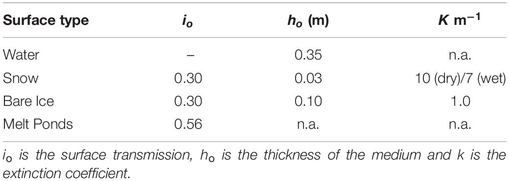
Table 1. Values of the parameters used in this study (based on adjustment to Green Edge observations, see Lebrun, 2019).

FIGURE 1

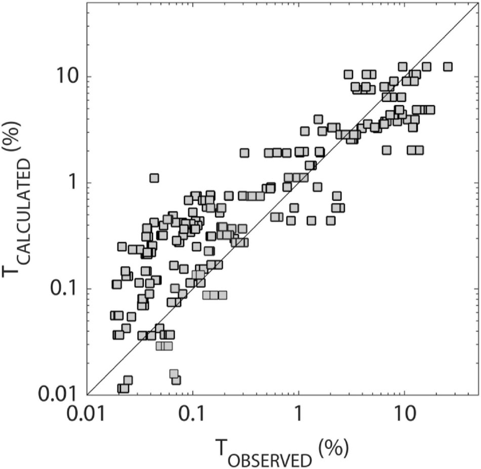
Figure 1. Calculated versus observed transmittance (T), based on environmental and optical observations from the Green Edge field operations (two fast ice camps, one drift ice cruise in spring and summer 2015–2016, N = 258; Oziel et al., 2019; Randelhoff et al., 2019). Observed transmittance is the ratio of irradiance under sea ice to that above sea ice, both from radiometers deployed in situ. Calculated transmittance derives from equations 1–4, using observed values of snow and ice thicknesses, air temperature and melt pond coverage, and with input parameters from Table 1.

Note, for snow there are two values used, one for a dry snowpack and one for a wet snowpack (i.e., melt has begun). Note also that the thickness of the near-surface high scattering layer is assumed as 3 cm for snow and 10 cm for ice. However, the thickness of snow and ice can be less than these values. Observational evidence for attenuation in very thin snow and ice is sparse. To regularize attenuation in very thin snow and ice we assume it to be equivalent to the attenuation in the fully developed near-surface high scattering layer (h₀ = 0.03) but reduced in proportion to the actual thickness.

Conversion From Solar Energy to Visible Quanta

Photosynthesis estimates rely upon photon counts in the visible wavelength range (Q_PAR, μE/m²/s, 0.4–0.7 μm) rather than upon solar energy in the solar waveband (F_SW, W/m², 0.2–4 μm). Both are tightly (practically linearly) related, hence the conversion from one to another is straightforward and often used in Earth System model applications. The relationship between Q_PAR and F_SW can be decomposed as follows: (1) the conversion from solar to visible energy, (2) the conversion from energy to quanta. Formally, one gets:

$$Q_{PAR}=\frac{F_{PAR}}{F_{SW}}\cdot \frac{Q_{PAR}}{F_{PAR}}\cdot F_{SW}(5)$$

where F_PAR/F_SW and Q_PAR/F_PAR can practically be considered as constants. Visible energy, visible quanta and shortwave energy fluxes are defined as (Morel and Smith, 1974):

$$F_{PAR}={\int }_{400nm}^{700nm}{E}_{\mathrm{\lambda }}\mathit{d}\lambda (6)$$

$$F_{SW}={\int }_{300nm}^{3000nm}{E}_{\mathrm{\lambda }}\mathit{d}\lambda (7)$$

$$Q_{PAR}={\int }_{400nm}^{700nm}{E}_{\mathrm{\lambda }}\frac{\mathrm{\lambda }}{hc}\mathit{d}\lambda (8)$$

In temperate marine environments, these relationships are well constrained. The ratio of PAR to solar energy ranges overF_PAR/F_SW = 0.45–0.50, according to simulations with a radiative transfer model (Frouin and Pinker, 1995; Frouin and Murakami, 2007). A classical value for the visible quanta-to-energy ratio is Q_PAR/F_PAR = 4.60 ± 0.03 J/μE (right under sea surface) decreasing to an average 4.15 J/μE within interior waters, based on a compilation of observations in temperate oceans (Morel and Smith, 1974). Therefore, over the ice-free fraction of the pixels, we use:

$$Q_{PAR}=0.50\times 4.60F_t(9)$$

In ice-covered environments, however, differences arise because of the presence of sea ice. Indeed, both ratios depend on the light spectral distribution, which is altered by snow and biogenic particles in sea ice. GreenEdge data offers a means to evaluate these relationships in ice-covered environments (Figure 2). GreenEdge spectral irradiance (W/m²/nm) observations feature 19 channels, with 10 nm bandwidth. Raw data were interpolated on 1-nm-wide bands, covering a reasonable part of the full shortwave range (320–800 nm).

FIGURE 2

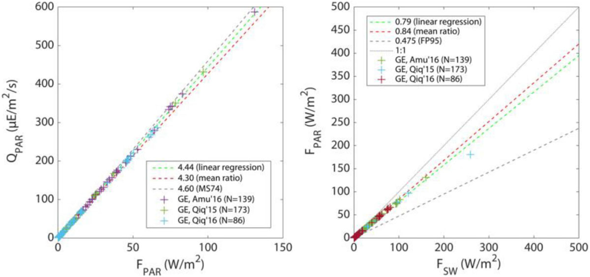
Figure 2. Observational constraints on the conversion from solar energy to visible quanta in ice-covered environments, based on spectral irradiance observations collected in the framework of GreenEdge (GE) program (+), and as retrieved from linear fits (lines). The left panel depicts the relationship in the visible range between quanta (Q_PAR) and energy (F_PAR). The right panel depicts the relationship between energy in the visible range (F_PAR) versus energy in the solar range (F_SW). Observational values (+) are split between the two landfast sea ice camps in Qiqitarjuak (Qiq’15 and Qiq’16) and the drift ice cruise onboard the R/V Amundsen in Baffin Bay (Amu’16). Linear fits use coefficients corresponding to observation-based values (linear regression coefficient and mean ratio) and to classically used values, corresponding to open water situation (Morel and Smith, 1974, MS74; and Frouin and Pinker, 1995, FP95).

Under fast and pack ice environments, both relationships (Q_PAR/F_PAR, F_PAR/F_SW) are nearly perfectly linear (R² = 0.999, 0.994). The quantum-energetic ratio is slightly smaller than for ice-free waters: Q_PAR/F_PAR = 4.44 ± 0.005μE/J. This is because the spectrum is shifted toward blue / green wavelengths, where photons are more energetic, hence one needs less photons per unit energy. A much clearer difference is that the fraction of energy in the visible is F_PAR/F_SW = 0.79 ± 0.003, i.e., much larger than in ice-free waters, because of the strong attenuation power of ice and snow for infrared radiation. Based on these considerations, over the ice-covered fraction of the pixels (regardless of the presence of snow or melt ponds), we use:

$$Q_{PAR}=0.79\times 4.44F_t(10)$$

Data Products

While several satellite-derived sea ice data sets now exist, many do not cover a long time-period, or cover the pan-Arctic region. In this paper we attempt to map light under the ice with currently available state-of-the art light parameterizations and pan-Arctic sea ice and snow products. Given the lack of pan-Arctic SIT information in summer, an important caveat is that we remain limited to the cold season and monthly means, while albedo, snow depth and ice concentration are all available at higher temporal resolution: daily to twice-daily time-steps. Further, pan-Arctic ice thickness estimates are currently limited to monthly means from satellites such as CryoSat-2. Finally, while some limited estimates of lead fractions and surface roughness exist, they are not available at the same temporal and spatial resolution needed for this study. Thus, in our snow depth distributions discussed below, we assume snow accumulated over level sea ice, though snow is redistributed and sublimated with winds (see Liston et al., 2020). The key data sets used are described below and will provide information on snow depth, SIC, SIT, surface albedo, incoming solar radiation and whether or not the snowpack is wet or dry.

Albedo and Solar Radiation

Visible satellites have provided observations of visible reflectance for several decades. A key sensor, the Advanced Very High Resolution Radiometer (AVHRR) has flown on several NOAA POES satellites, providing the potential to map surface albedo as far back as October 1978. AVHRR carries one visible channel, one near-infrared channel, one mid-infrared and two thermal infrared channels, from which surface albedo and surface temperature can be determined.

The AVHRR Polar Pathfinder Extended (APP-X) data set (Key et al., 2019), produces twice-daily (ascending and descending passes) estimates of broadband shortwave surface albedo for both polar regions. Here we use the data corresponding to local time of 14:00 GMT (ascending pass). While the surface can only be viewed during clear-sky conditions, a cloud masking algorithm and radiative transfer modeling is used to provide an all-sky (e.g., clear or cloudy) albedo at every satellite pixel. Further, this radiative transfer modeling is used to infer the daily averaged incoming solar radiation at the ground. Early evaluation of the data product was performed through comparisons with in situ observations collected during the yearlong Surface Heat Budget of the Arctic Ocean (SHEBA) experiment (Moritz et al., 1993). Results were summarized by Key et al. (1997). In short, biases with incoming solar radiation were on the order of 9.8 Wm^–2, whereas surface albedo comparisons revealed a bias of 0.028 for the all-sky albedo. Clear-sky albedo conditions had smaller mean errors. While these errors were previously assessed, it is likely that the bias in albedo is larger than what was reported previously. Data for both variables are provided daily on a 25-km equal-area (EASE) grid.

Sea Ice Concentration and Timing of Melt Onset

Since the late 1970s, there have been a series of multi-frequency passive microwave sensors launched that today provide more than 40 years of brightness temperatures that can be used to map sea ice given the large dielectric contrast between open water and ice. Starting with the launch of the Nimbus-7 SMMR instrument in October 1978, and followed on with successive DMSP SSMI instruments (since July 1987) there have been daily (twice daily for SMMR) observations of the polar regions at a nominal spatial resolution of 25 × 25 km². While several algorithms exist for retrieving SIC from these brightness temperatures (e.g., see Ivanova et al., 2015), we rely on the NASA Team sea ice algorithm (Cavalieri et al., 1997). This algorithm is produced in near-real-time by the National Snow and Ice Data Center (Fetterer et al., 2017).

While the accuracy of the SICs is generally high during the cold season, during summer its precision is downgraded due to liquid melt water on the snow and/or ice surface that causes the NASA Team algorithm to underestimate the true SIC as these areas will be interpreted as open water. As we are currently limited to the cold season because of the lack of SIT information once melt begins, the choice of algorithm is less important. Importantly, the sensitivity of the microwave emissivity to liquid water in the snowpack provides a means to flag if the melt has begun using the approach of Markus et al. (2009). Both the melt onset and SIC data sets are provided on a 25-km Polar Stereographic grid. All data sets are re-gridded to a 25-km equal area (EASE) grid.

Snow Depth

Snow depth has not been routinely observed from satellites. Some studies have relied upon passive microwave brightness temperatures used in the SIC algorithms to detect snow depth over first-year ice regions (e.g., Markus and Cavalieri, 1998; Comiso et al., 2003), yet results yield unrealistic snow depths in regions when snow melt has started and along the marginal ice zone (Stroeve et al., 2020). Other efforts have involved using atmospheric reanalysis data to model snow accumulation over sea ice, using simple (e.g., Kwok and Cunningham, 2008; Petty et al., 2018) to more sophisticated snow models (Liston et al., 2018, 2020). These have been implemented in either a Eulerian (Petty et al., 2018) or Langrangian framework (Kwok and Cunningham, 2008; Liston et al., 2020; Stroeve et al., 2020).

In this study we rely on SnowModel-LG (Liston et al., 2020) to generate snow-depth. SnowModel-LG is a spatially distributed snow-evolution modeling system that has previously been demonstrated to be capable of simulating high-resolution snow accumulation around ridges and snow dunes (Liston et al., 2018), and has recently been applied to map snow depth and density on a pan-Arctic scale using satellite-derived ice motion vectors in a Lagrangian framework (Liston et al., 2020; Stroeve et al., 2020). In short, SnowModel-LG consists of 4 sub-models:

(1) EnBal (Liston, 1995; Liston et al., 1999) calculates surface energy exchanges and snowmelt; (2) SnowPack-ML (Liston and Hall, 1995; Liston and Mernild, 2012) is a multi-layer snowpack model that simulates snow depth, density, grain size, and habit (e.g., wind slab, depth hoar), and temperature evolution of each storm-related layer. Density evolves as a function of air temperature, overburden pressure, time, and the presence of blowing snow (Liston and Hall, 1995; Liston et al., 2007). The latest version adds vapor-flux related metamorphism responsible for growing faceted crystals and depth hoar (Liston et al., 2020);

(2) SnowTran-3D (Liston and Sturm, 1998; Liston et al., 2007) simulates formation and distribution of snowdrifts that develop around topographic obstructions to wind. It simulates the horizontal snow-transport flux at each time step, as a function of surface shear stress from the wind, surface shear strength of the snow, and amount of snow available for transport; and

(3) SnowDunes (Liston et al., 2018) simulates high-resolution snow surface features such as dunes and sastrugi. Ice motion vectors derived from satellite play a key role in redistributing the snow for the pan-Arctic simulations.

In this study we use the daily snow depth and density product generated from MERRA-2 atmospheric reanalysis (Gelaro et al., 2017) together with ice motion vectors from Version 4 of the Weekly EASE grid sea ice motion vector data set (Tschudi et al., 2019). Comparison against various in situ data sets show SnowModel-LG simulations capture the observed spatial and temporal variability of snow accumulation (Stroeve et al., 2020). The data set spans August 1980 through July 2018 and is offered, as with the other products used, on the 25-km EASE grid.

Sea Ice Thickness

While we have more than 40 years of SIC observations from satellite, we do not have a similarly long-term SIT data set. Several satellite missions have provided insight into SIT using either radar (e.g., ERS1/2, Envisat, CryoSat-2) or laser altimetry (ICESat-1/2), though they are not consistent in time or spatial area covered. In this study, we focus on the 9 years of continuous ice thickness observations from CryoSat-2. As before, several different algorithms exist to retrieve SIT from CryoSat-2 (e.g., Kurtz et al., 2014; Tian-Kunze et al., 2014; Hendricks et al., 2016; Lee et al., 2016; Kurtz and Harbeck, 2017; Ricker et al., 2017; Tilling et al., 2018). Note that CryoSat-2 does not measure SIT directly but measures the ice freeboard, which together with snow depth, snow density and ice density can be converted into SIT. In this study we chose to use a new algorithm developed by Landy et al. (2020), which uses a Lognormal Altimetry Retracker Model (LARM) applied to CryoSat-2 returns, together with snow depth and snow density from SnowModel-LG to estimate SIT. The LARM algorithm is based on simulations of CryoSat-2 waveforms performed with a physical model for the SAR altimeter echo backscattered from sea ice (Landy et al., 2019). The physical echo model accounts for realistic variations in the sea ice surface roughness and radar backscattering properties, at the scale of the CryoSat-2 footprint, which affect the derived sea ice freeboard. Since SnowModel-LG has been run with both MERRA-2 and ERA-5 atmospheric reanalysis, an average of both is taken to represent the snow depth and density in the SIT-retrieval. Data are provided monthly on the 25 km EASE grid.

Use of a Heterogeneous vs. Homogeneous Snow Depth and Ice Thickness Distribution

An important issue to be aware of when using mean snow depth and ice thickness products for light transmission is that at 25-km grid scales, observations clearly show that snow depth and SIT do not follow simply mean values per grid cell (i.e., h_i and h_s). They instead follow a probability density distribution (PDF) with varying widths of distributions depending on time of year and ice type (e.g., Renner et al., 2013). Since thin ice or thin snow cover play an important role in light transmission we would underestimate light transmission by simply assuming mean values for h_s and h_i. In terms of SIT, models often parameterize the sub-grid-scale SIT variations by replacing h_i by an ice thickness distribution (Thorndike et al., 1975) that has been discretized using fixed PDFs per thickness category (Hibler, 1984). However, several studies have highlighted the fact that ice thickness may have more than one mode, with bimodal distributions found in regions with both first-year and multiyear ice present (e.g., Haas et al., 2010). Based on airborne electromagnetic induction sounding (EM-bird) measurements reported in Haas et al. (2010), Castro-Morales et al. (2014) evaluated the impact of using 15 ice categories on the surface heat budget in the Arctic Ocean. This representation of ice thickness resolves more thin ice than the flat (e.g., same probability) seven thickness categories used in some sea ice models. Because not enough is known as to how ice thickness distributions may be changing as the ice cover has thinned and become more mobile (e.g., Rampal et al., 2009), we decided to model the ice thickness distribution through 15 ice thickness categories following Castro-Morales et al. (2014), such that the ice thickness is distributed between 0 and a thickness of 3h_i with a bin width of 3h_i/15 = 0.2h_i.

As we have for SIT, snow depth is highly heterogeneous at small spatial scales.

Abraham et al. (2015) show for example that, for the same mean snow depth, this small-scale heterogeneity tends to increase transmission below sea ice because of the large contribution of thin snow. They tested various distributions (gamma, Rayleigh) and compared them to the assumption of a snow distribution between 0 and twice the mean snow depth, showing little difference. Thus, in this study we also assume a snow distribution similar to ice thickness but instead solve for the integral of the probability density function g(h_s). For example, if we just consider the snow transmittance and assume snow is homogenous with mean thickness, the snow transmittance can be given by:

$$T_s=i_o[1-a(\overline{h_s})]\cdot \exp (-k_s{\overline{h}}_s)(11)$$

To account for the fact that snow is heterogeneous, characterized by g(h_s) we can write:

$${\int }_0^{\mathrm{\infty }}g(h_s)\mathit{d}{h}_s=A(12)$$

where A is snow concentration or area (fraction of grid-cell covered by snow). The first moment of g(h_s) is the mean thickness:

$${\int }_0^{\mathrm{\infty }}g(h_s)h_s\mathit{d}{h}_s=\overline{h_s}(13)$$

Using, the first integral above (Eq. 11) one then gets:

$$g(h_s)=A/(2\overline{h_s})(14)$$

Calculating transmittance with g(h_s), we get:

$$\overline{T_s}=\frac{i_0}{2\overline{h_s}}{\int }_0^{2\overline{h_s}}[1-\mathrm{\alpha }(h_s)]\cdot \exp (-k_s{h}_s)\mathit{d}{h}_s(15)$$

Many models assume that thin ice has a thinner snow pack, yet we lack the observations to fully support this assumption. Since we do not fully understand how snow depth distribution depends on ice thickness distribution we instead solve the full snow distribution per ice thickness category. Thus, including the ice thickness per thickness category h_i,n, we obtain:

$$\overline{T_{s,n}}=\frac{i_0}{2\overline{h_s}}\exp (-k_i{h}_{i,n}){\int }_0^{2{\overline{h}}_s}[1-\mathrm{\alpha }(h_s)]\exp (-k_s{h}_s)\mathit{d}{h}_s(16)$$

Implementation

Below we implement our transmission and PAR calculations using the monthly mean satellite products. Since there is little to no light during the winter months (November, December, and January), we focus on the months of October, February, March, and April for which there is some daylight along the sea ice pack margins (October and February) up to the point where there is daylight on a monthly pan-Arctic scale (March and April). To evaluate the influence of daily snow depth and albedo variability on under-ice PAR, we additionally fix the SIT based on the previous monthly mean, and change it at monthly time-steps from February to April for each year at three different locations, centered at the following locations but for a 5 × 5 grid cell area (or 125 km by 125 km): Chukchi Sea (72.97N/−171.29E); Beaufort Sea (78.45N/−150.23E); Laptev Sea (77.09N/119.79E). We implement both the homogenous snow and ice cases and heterogeneous distributions as discussed above, and examine their influence on the under-ice PAR. Further, since we have snow depth and albedo estimates through the summer seasons, we additionally investigate snow depth and albedo trends from 1982 to 2018 on light transmission to the top of the ice (i.e., through the snowpack) in February through July.

We conclude with a discussion on uncertainty of satellite and transmission parameters on the results. Specifically, for each month we additionally estimate locally the error in under-ice light transmittance as a function of uncertainty in the physical sea ice/snow parameters (ice thickness, snow depth, surface albedo, and SIC) as well as the attenuation properties (Table 2). These uncertainties are considered with respect to errors in the satellite retrievals (snow depth, albedo, ice thickness, and ice concentration) as well as the parameters used in the light calculations and are based on current knowledge. For the albedo, we assume an uncertainty of 0.05, higher than the accuracy reported in the APP-X data set, as a result of problems in handling the anisotropic reflectance of snow, particularly under large solar zenith angles (i.e., February). At the ice edge however, the errors may be larger given the fact that the ice edge is not well-resolved from passive microwave satellite data, and thin ice limitations from CryoSat-2 become important. This is discussed further in section “Appropriateness of Methodology.”

TABLE 2

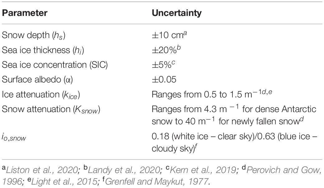
Table 2. Uncertainties used for sensitivity analysis of under-ice PAR to uncertainties in sea ice/snow physical properties and attenuation properties used in the Beer–Lambert approach.

Results

Pan-Arctic Under-Ice Light

Monthly mean (February to April and October) summaries of under-ice PAR, transmittance and the various input data from 2011 to 2018 are summarized in Figures 3–9, respectively. All of these results include both the snow and ice distributions as described in Section “Data Products.” The impact of using our modeled snow depth and thickness distributions compared to mean values per grid cell are discussed in section “Impact of Homogeneous vs. Heterogeneous Snow Depth and Ice Thickness Distributions.”

FIGURE 3

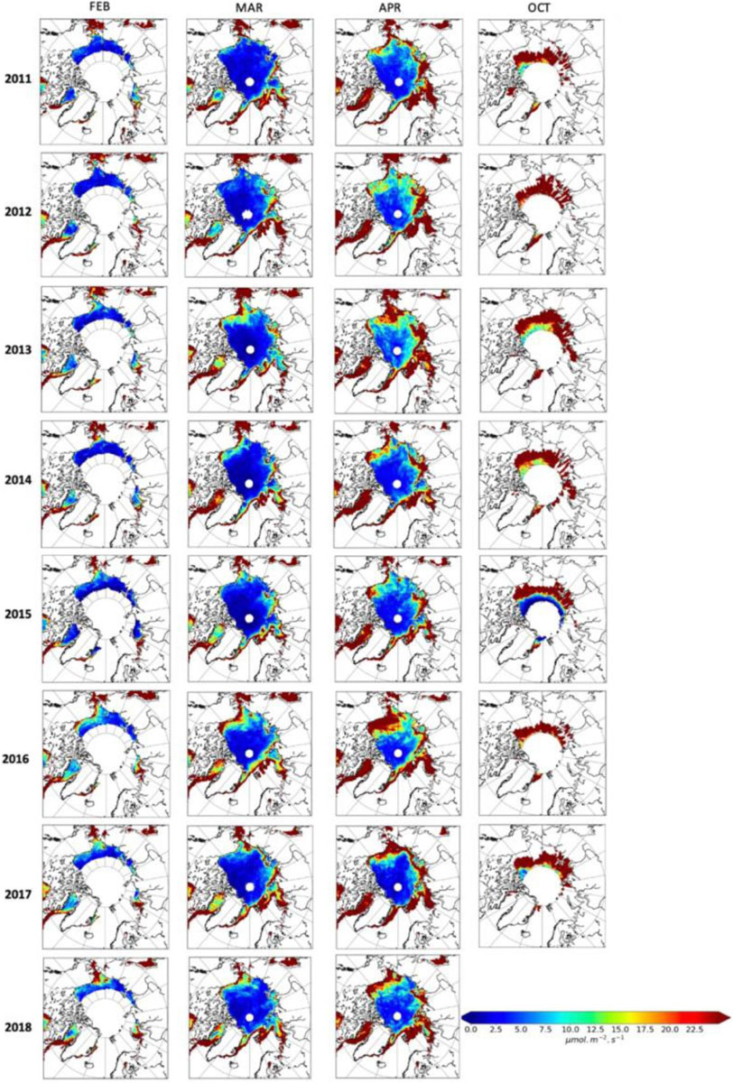
Figure 3. Summary of the monthly mean under-ice PAR maps produced using the satellite-derived sea ice and modeled snow depth data for all months and all years from February 2011 to April 2018.

FIGURE 4

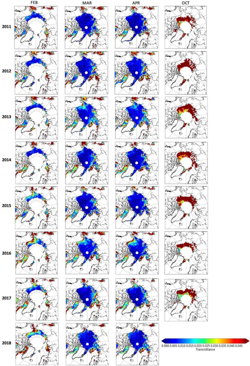
Figure 4. Summary of the monthly mean transmittance produced using the satellite-derived sea ice and modeled snow depth data for all months and all years from February 2011 to April 2018.

FIGURE 5

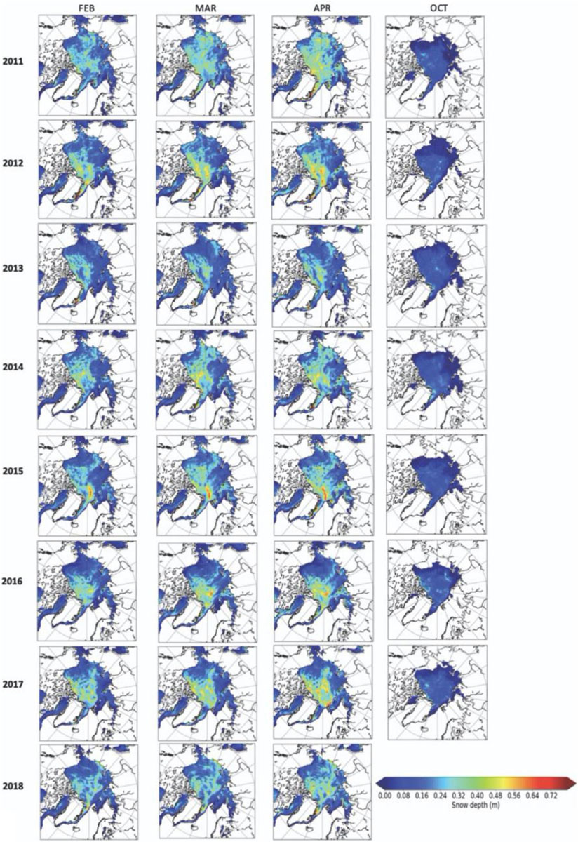
Figure 5. Summary of the monthly mean snow depth for all months and all years from February 2011 to April 2018.

FIGURE 6

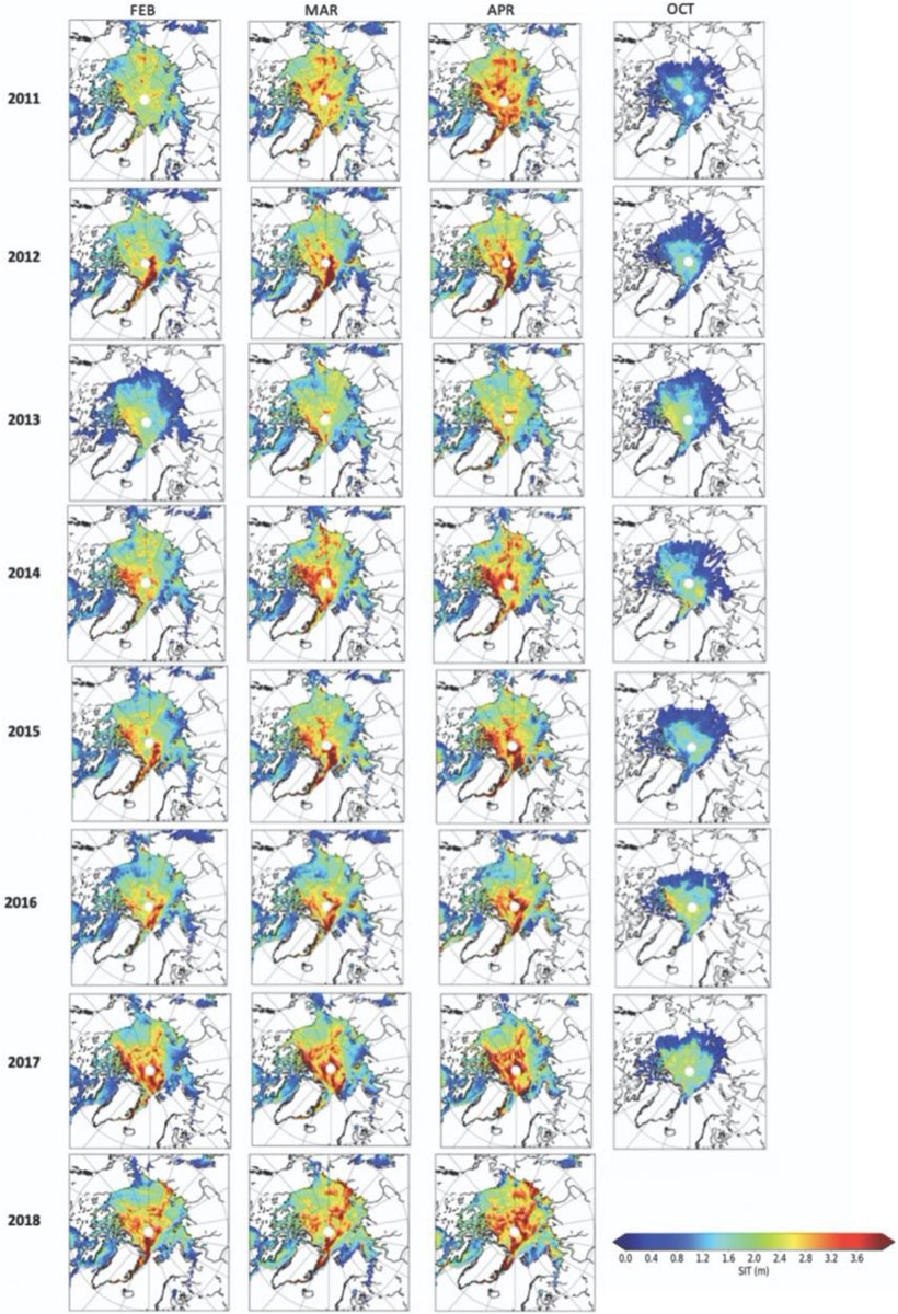
Figure 6. Summary of the monthly mean ice thickness for all months and all years from February 2011 to April 2018.

FIGURE 7

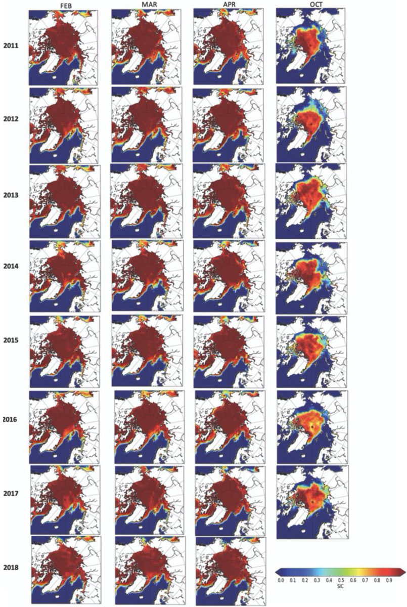
Figure 7. Summary of the monthly mean sea ice concentration for all months and all years from February 2011 to April 2018.

FIGURE 8

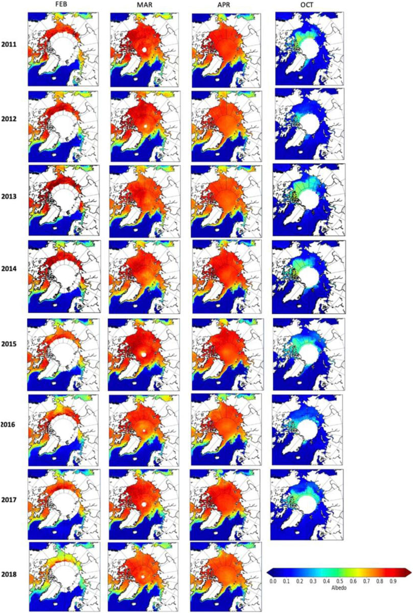
Figure 8. Summary of the monthly mean surface albedo for all months and all years from February 2011 to April 2018.

FIGURE 9

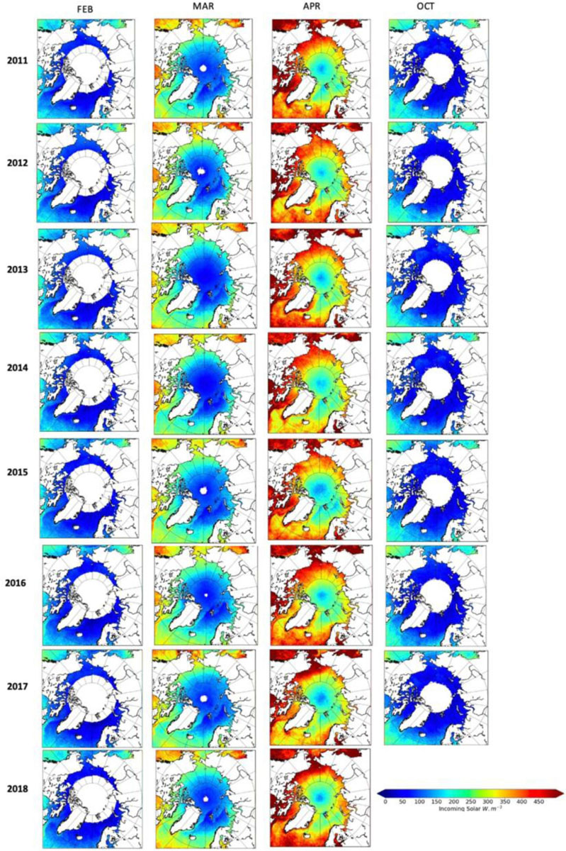
Figure 9. Summary of the monthly mean incoming solar radiation for all months and all years from February 2011 to April 2018.

Some key results stem from these maps. First, in April there is a substantial amount of under-ice PAR (>10 μmol m^–2 s^–1) entering the Arctic ocean in the southerly locations (Figure 3). This is expected as there is more incoming solar radiation in these locations compared to the central Arctic and seasonally more in April than the other months evaluated. There is also less snow in these regions, often less than 8 cm, which combined with incoming solar radiation in excess of 400 Wm^–2, allows for a larger light transmission (Figure 4) and therefore, under-ice PAR.

Second, interannual variations in the under-ice PAR are strongly linked to the snow depth variability (Figure 5). This is particularly true from February to April, whereas SIT largely contributes to October under-ice PAR variability (Figure 6). The lowest pan-Arctic snow accumulation in April for example occurred in 2013, resulting in an increase in under-ice PAR over larger parts of the central Arctic Ocean compared to other years (e.g., 4–10 μmol m^–2 s^–1 compared to on average 2–5 μmol m^–2 s^–1). Conversely, in 2011, snow depths across large parts of the Arctic Ocean exceeded 35 cm, which in turn limited the under-ice PAR to values less than 10 μmol m^–2 s^–1 most everywhere in the central Arctic. Spatially, interannual variability of under-ice PAR is large in the Beaufort Sea, reflecting large variations in snow depth in this region (e.g., compare 2016 to 2011).

While there is less light in February and March, thin snow and ice thickness in regions such as the Bering Sea, Sea of Okhotsk and Baffin Bay already allow for increased light transmittance and under-ice PAR values exceeding 20 μmol m^–2 s^–1. Similarly, in some years, under-ice PAR in the Chukchi and Beaufort seas are seen to increase to above 10 μmol m^–2 s^–1 already in February. Hancke et al. (2018) have recently showed that net growth in ice algae could be initiated at irradiances lower than 0.17 μmol m^–2 s^–1. Based on other studies, threshold values for onset of algal growth are in the range of 0.5–5 μmol m^–2 s^–1 (see Letelier et al., 2004; Tremblay and Gagnon, 2009; Leu et al., 2015). These maps suggest that light levels are higher than the lower threshold value in February for almost all regions of the Arctic Basin. This suggests that algal growth can start even at this early state in the season. If one considers a higher threshold than 0.17 μmol m^–2 s^–1 (e.g., Hancke et al., 2018), we find that, algal growth would happen between February and March at lower latitudes, then move northward in April, without reaching regions further north than 85° N. Only in 2012 and 2013 did light levels in the high Arctic (above 85° N) become large enough to initiate algal growth in April.

How do these results compare to published values? In the months of February to April, transmittance values remain below 0.01 in most of the Arctic, except for the shelf areas, where thinner ice and snow cover allow for larger transmittance values. In October, when ice is thinner and not much snow accumulated yet after summer melt, transmittance values are larger than 0.025. In situ measurements of light transmission before April–May are not available. However, in a recent compilation of under-ice light measurements, Katlein et al. (2019) report values of transmittance that do not exceed 0.01 in May. This is in agreement with the present estimations, except for the marginal areas. In these cases, though, the estimated transmittance values are still in the range of variability shown by Katlein et al. (2019) for the late spring-summer period. Between late April and early June (i.e., before melt onset), reported values of light transmittance range between 0.0006 and 0.003 (see Supplementary Figure S8 in Oziel et al., 2019), in agreement with the present results of T < 0.01. Another newly published data set described in Castellani et al. (2020) and available on PANGAEA¹ shows a mode at transmittance values in May and June below 0.05, again in agreement with the estimates presented in this study.

Daily Evolutions From February to April 2012

As shown above, the use of the monthly means of each physical parameter gives a good evaluation of inter-annual changes in under-ice PAR on a monthly basis. However, for the timing of a bloom, daily estimates are preferred. Here we evaluate the influence of daily variations in snow depth and albedo on the under-ice PAR, but fixing the SIT to the monthly mean values and following the daily evolution of snow depth, incoming solar radiation and surface albedo. In particular, we are interested in when the daily PAR value increases above the threshold range of 0.5–5 μmol m^–2 s^–1. In other words, when plankton is susceptible to be more active. Such a light threshold value is purely indicative, since a light threshold for net photosynthesis is not well observationally constrained or even well justified. Depending on the value of the threshold in the explored range and on the rate of change in irradiance, the alleviated onset of algal activity varies by days to a few weeks.

Figure 10 shows the evolution of the under-ice PAR from 1 February to 30 April 2012, as well as the corresponding evolution of the snow depth and the albedo, for three randomly chosen locations in the Chukchi (72.97N/−171.29E), Beaufort (78.45N/−150.23E), and Laptev (77.09N/119.79E) seas. Note since the albedo and incoming solar radiation are centered around 14:00 GMT, these values represent the evolution at this time of day. Also shown is the algal growth range threshold (gray shading) based on Letelier et al. (2004) and Tremblay and Gagnon (2009). First, and as expected, we can observe the important day-to-day variations in amplitude of both snow depth and albedo and the influence these have on the under-ice PAR. Second, we notice the impact of the spatial variability of snow depth on the range of amplitude of the under-ice PAR between regions. As also shown in the monthly maps (Figure 9), less snow in the Laptev Sea compared to the Beaufort and Chukchi seas results in a substantial increase of the under-ice PAR earlier in the year. Finally, already by the end of February, the amount of under-ice PAR exceeds the lower threshold for initiating algal growth within the Chukchi Sea, though this is strongly controlled by the amount of snow on the ice and the albedo. In the Beaufort and Laptev sea locations, the lack of sunlight delays the timing of light under the ice until March, however, once there is sunlight, the under-ice PAR within the Laptev Sea location almost already exceeds the higher threshold for initiating algal bloom as the snow cover is considerably thinner than in the Beaufort Sea.

FIGURE 10

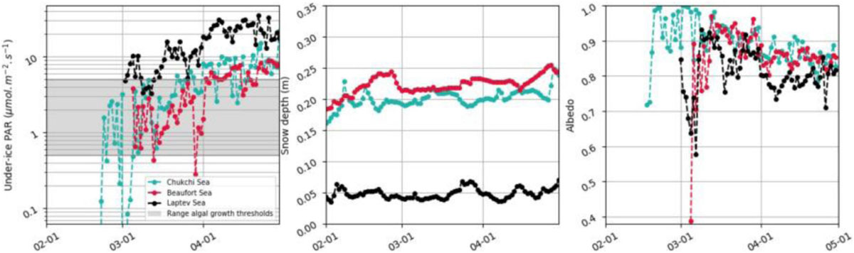
Figure 10. Daily retrieval of the under-ice PAR using daily evolutions of the physical parameters starting on February 1 2012. Parameters shown are the snow depth and the albedo. Three locations are evaluated for a 5 × 5 pixel area around each center location: Chukchi (72.97N/−171.29E), Beaufort (78.45N/−150.23E), and Laptev (77.09N/119.79E) seas. Gray shading corresponds to range of thresholds for algal growth (0.5–5 μmol m^–2 s^–1).

Impact of Homogeneous vs. Heterogeneous Snow Depth and Ice Thickness Distributions

Here we examine the impact of computing light transmittance through a heterogeneous snow depth and SIT distribution compared to assuming mean snow depth and ice thickness values per 25-km grid cell. For these comparisons, we use a mean SIT per grid cell to only examine the snow distribution impact, and vice versa, a mean snow depth to examine the influence of the SIT distribution. Further, only the month of April is shown as it is the month with the largest amount of light transmission through the ice prior to melt onset. While results are largely insensitive to year, years with thinner snowpack, or thinner ice will show overall larger effects of including a distribution versus mean values.

As expected, for both the ice thickness and snow depth distributions, the amount of under-ice PAR increases compared to using mean values per grid cell (Figures 11, 12). This is because thin ice and snow transmit much more light than thick ice and snow. With our parameterizations, the mean transmission is always higher than the transmission calculated with mean thickness — a result already obtained by Abraham et al. (2015) — in turn increasing the overall under-ice PAR for each grid cell. Nevertheless, the differences in under-ice PAR remain small, especially over the central Arctic where PAR increases just slightly, between 0 and ∼2 μmol m^–2 s^–1 (∼5% relative difference, or percentage of the average under-ice PAR it represents). Castellani et al. (2017) report a threshold value for algal bloom of 1.78 μmol photons m^–2 s^–1 which is at the upper boundary of the differences of PAR in the central Arctic. The effect of using mean values per grid cell thus does not have large effects on algal bloom, at least in the central Arctic. It is different for coastal regions in the Arctic basin and also in the Barents Sea, characterized by generally thinner snow cover as well as thinner ice, where differences in under ice PAR are large enough (i.e., >5 μmol m^–2 s^–1, or >∼12.5% relative difference from the mean value) to impact the onset of algal bloom.

FIGURE 11

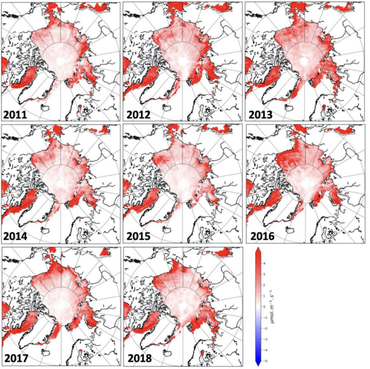
Figure 11. Difference in monthly mean April PAR between using a heterogenous snow depth following Eq. 12 and assuming a mean ice thickness per grid cell versus a mean snow depth per satellite pixel.

FIGURE 12

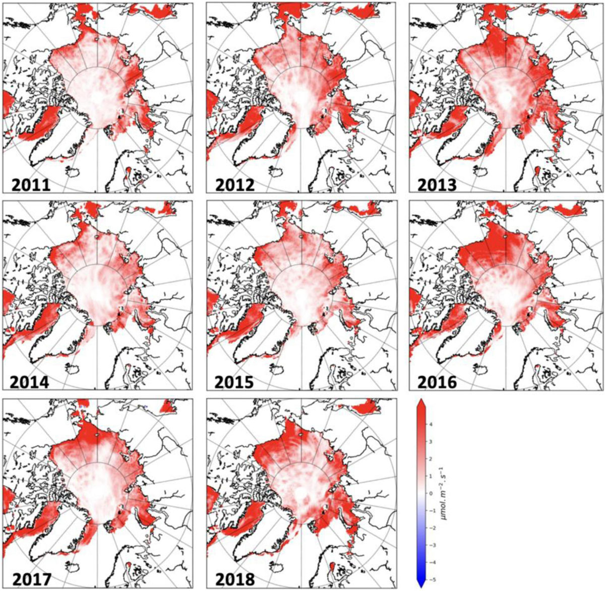
Figure 12. Difference in April PAR between using a mean sea ice thickness per satellite pixel versus a fifteen ice thickness categories ITD heterogeneously distributed between 0 and 3h_i, as described in section “Data Products,” and assuming a mean snow depth per grid cell.

In regards to snow depth, increases in under-ice PAR above 4 μmol m^–2 s^–1 (10% of relative difference) are found mostly outside of the Arctic basin (i.e., Bering Sea, Baffin Bay, Barents Sea), but also at times within the Chukchi and Beaufort seas, as well as the Laptev and Kara seas that can reach 5 μmol m^–2 s^–1 (12.5% relative difference) or more. The largest increases in under-ice PAR within the Beaufort Sea are found in 2016, when there was relatively more transmittance of light as a result of less snow accumulation compared to other years (see also Figures 2, 4). Thus, the impact of using a snow depth distribution varies from year to year, depending on the average snow depth per pixel.

Similarly, for the ice thickness distribution versus mean SIT values we observe that larger differences on the order of at least 4 μmol m^–2 s^–1 occur when the sea ice is thinner, as for example close to the shelf but also in the Chukchi and Beaufort seas, especially during 2013, 2016, 2017, and 2018. As for Figure 10, April 2016 is the year when the differences between the SIT distribution and mean SIT per pixel are greater, especially in the Chukchi Sea with more than 5 μmol m^–2 s^–1 difference. This is due to the fact that for this year, the ice is overall thinner than for the other years. During some years and regions, the sub-grid scale SIT distribution results in larger increases in under-ice PAR compared to sub-grid scale snow depth distribution (i.e., 2013 in Chukchi and Laptev seas), and in others the reverse is true (i.e., 2012 and 2015 in Beaufort Sea). Considering the threshold reported by Hancke et al. (2018), these sub-grid scale variations in snow depth and ice thickness may be important in terms of timing of under-ice algal growth and thus more research on how best to represent sub-grid scale snow depth and ice thickness distributions is warranted, especially during this transition from a multiyear to first-year dominated Arctic Ocean, with corresponding changes in surface roughness.

Impact of Snow Depth Trends on Transmission Through Snow

So far, our assessments have focused on the CryoSat-2 time-period and during the time of the year for which thickness observations are available. To assess longer term changes in light availability, not just in autumn and spring, but also in summer, we can examine how changes in snow depth and surface albedo are impacting the amount of light transmitted to the top of the ice (i.e., through the overlying snowpack). In particular, we are interested in the impacts of changing snow accumulation on light availability when light first becomes available and until the snow melts off the ice. Figure 13 shows trends from 1982 to 2018 in SnowModel-LG snow depths forced with MERRA-2 atmospheric reanalysis from February through July (see also Stroeve et al., 2020). Overall, winter and spring snow depth is found to be declining throughout the Arctic Ocean marginal seas, with slightly positive trends north of Greenland. In particular, statistically significant negative trends (at 95% confidence interval) are seen throughout the Beaufort, Chukchi, East Siberian, Laptev, Kara and Barents seas in February to May (between 2 to 8 cm per decade, depending on location), that increase to cover most of the Arctic Ocean also in June, and the central Arctic in July. Positive trends (∼1–3 cm per decade) north of Greenland are not statistically significant, but agree with positive trends in albedo in this region (Figure 14). Since no trends in precipitation are revealed in the reanalysis precipitation themselves (Barrett et al., 2019), the reduction in snow depth in the marginal seas is most likely a result of later freeze-up and earlier melt onset (e.g., Stroeve and Notz, 2018) that reduce the time over which snow can accumulate, rather than a change in precipitation. It also reflects a reduction in multiyear ice, as the longer an ice parcel can accumulate snow, the deeper the snowpack tends to be (e.g., Liston et al., 2020).

FIGURE 13

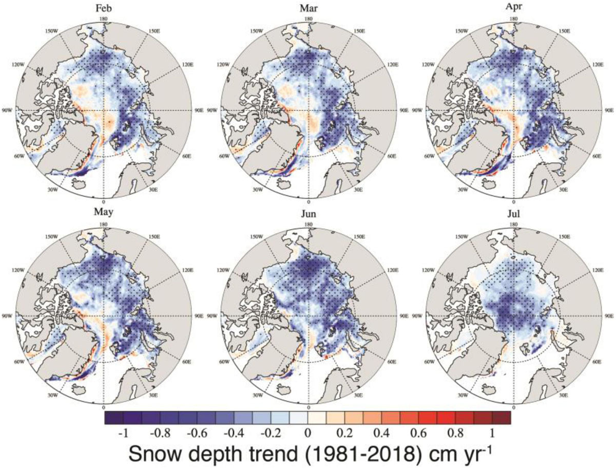
Figure 13. Snow depth trends (cm/yr) in February through July from 1982 to 2018 over Arctic sea ice as represented in SnowModel-LG (Liston et al., 2020) forced by MERRA-2 atmospheric reanalysis. Trends statistically significant at the 95% confidence level are indicated by black marks.

FIGURE 14

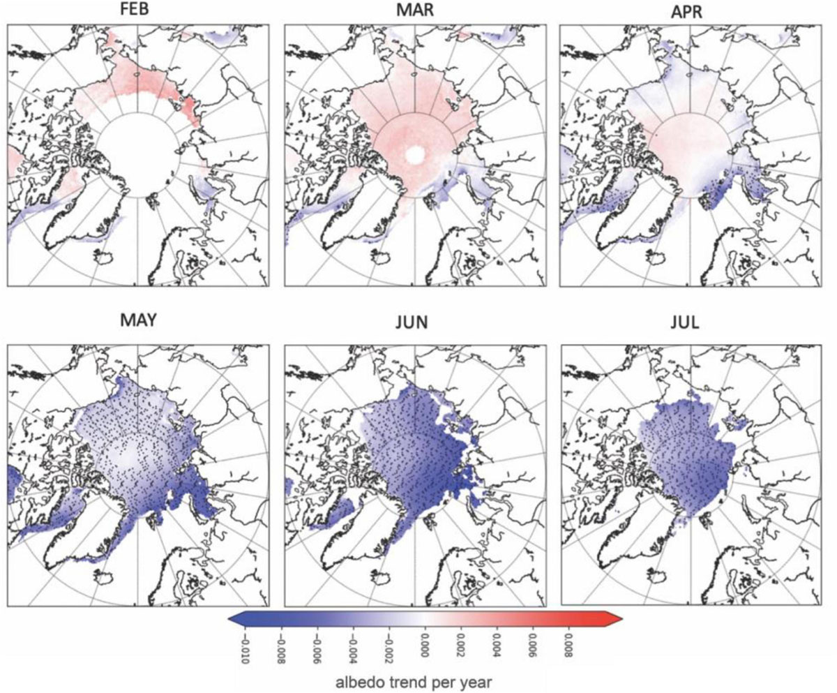
Figure 14. Albedo trends per year in February through July from 1982 to 2018 over Arctic sea ice as derived from AVHRR. Note albedo trends are given for open water as well as ice-covered regions and thus large negative trends along the ice margins reflect in part earlier development of open water, while trends over the icepack in summer reflect also melt pond development. Trends statistically significant at the 95% confidence level are indicated by black marks.

At the same time, and not surprisingly, the surface albedo also exhibits generally statistically significant negative trends over most of the Arctic basin in May, June, and July, reflecting earlier melt onset, earlier ice retreat (i.e., open water) and melt pond development. Negative albedo trends in February to April are mostly confined to the regions outside the Arctic basin (e.g., Baffin Bay, Barents and Bering seas). Negative albedo trends outside of the central Arctic prior to melt onset are largely the result of a lack of winter sea ice in more recent years, as the trends include both sea ice and open water regions. Small positive trends are also observed in February and March (∼0.02–0.06 per decade) over the areas with sunlight in the central Arctic, larger in February than in March. None of these trends are statistically significant, yet we do find they are consistent with slightly positive trends in snow accumulation that are statistically significant north of the Canadian Archipelago. On the other hand, positive albedo trends may also reflect problems in the albedo estimates during this time of year. As seen previously in Figure 10, albedo in 2012 is seen to reach nearly 1.0 in the Chukchi Sea in February which exceeds the albedo for new snow (0.90, Wiscombe and Warren, 1980). This likely points to a problem in properly accounting for the anisotropic reflectance of snow, especially under oblique solar and sensor zenith angles found at this time of year. Positive albedo trends (∼0.01 to 0.02 per decade) in April may also reflect changes in cloud cover. The APP-X data product produces an all sky albedo, whereby the amount of solar radiation underneath clouds is modeled based on estimated cloud top height, temperature and ice versus water clouds. Problems in accurately detecting cloud cover and cloud properties, combined with overall increases in springtime cloud cover (e.g., Wang et al., 2012) and cloud thickness (Huang et al., 2019) will influence the amount of incoming solar radiation as well as the surface albedo through modification of the spectral distribution of the incoming solar radiation (e.g., Grenfell and Maykut, 1977; Grenfell and Perovich, 2008).

The regions with negative snow depth trends, combined with negative albedo trends will play a significant role in increasing light availability under the ice. While we do not have ice thickness during that time, we can estimate how these snow depth changes, together with albedo changes, impact light transmission through the snow pack. These results are summarized in Figure 15. The largest positive trends in transmittance under the snow, exceeding 0.06 per decade are found in June in the Chukchi Sea and then everywhere there is sea ice in July. However, already in February small positive trends in under-snow transmittance are observed, that are statistically significant in the Chukchi Sea, in the East Greenland Sea and north of Novaya Zemyla (∼0.01 to 0.03 per decade). By April, statistically significant positive trends in under-snow transmittance occur throughout the marginal seas of the Arctic Ocean, reaching 0.04 per decade in the northern Barents Sea. This will cause a shift of the production season onset to earlier times in the spring in these regions. This will in turn affect the lower trophic levels, since there might be a mismatch between high food availability and events such as reproduction and spawning (Durant et al., 2007). Moreover, since the trend in snow cover is not uniform throughout the Arctic, this might lead to not only a temporal, but also a spatial shift of growth onset.

FIGURE 15

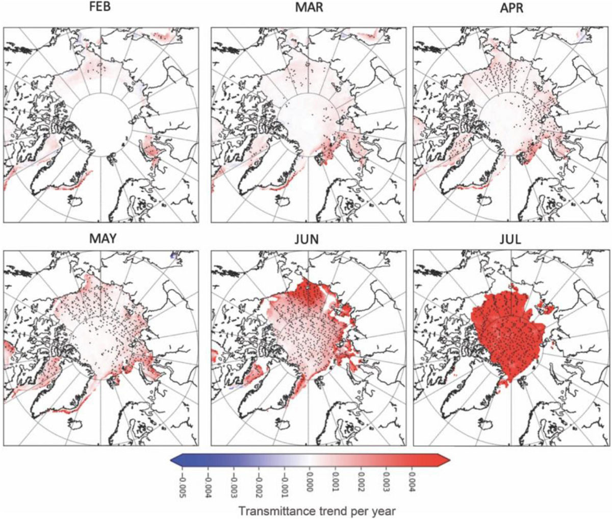
Figure 15. Under-snow transmittance trends per year computed using the albedo and snow depth in February through July from 1982 to 2018 over Arctic sea ice. Trends statistically significant at the 95% confidence level are indicated by black marks.

Uncertainty Analysis

As mentioned in section “Implementation,” we investigate the error of the under-ice PAR as a result of uncertainty on the physical sea ice/snow parameters used to compute the light transmission as well as the values used in the radiative transfer (Table 2). This evaluation was conducted for April of each year of the study and the resulting errors, averaged over the Arctic basin and for all 8 years (2011–2018) are summarized in Table 3. Overall, the uncertainty in the under-ice PAR from uncertainties in the physical sea ice or snow parameters ranges from ±1.5 to ±9.2 μmol m^–2 s^–1, or a relative error of ∼4–22%. The uncertainty of ±20% on the SIT, gives the lowest errors in the under-ice PAR, while an uncertainty of ±10 cm in snow depth gives the highest PAR errors. This is followed closely by a ±5% uncertainty in SIC with a 7.2 μmol m^–2 s^–1 or (17%) and ±0.05 uncertainty in the surface albedo, which results in 5.0 μmol m^–2 s^–1, or a relative error on the order of 12.2%. The larger impact of snow depth and albedo uncertainties relative to SIT on under-ice PAR agrees with Katlein et al. (2019), who found that ice thickness was an overall poor factor in determining overall light transmittance levels. Instead, snow cover was found to provide the primary limit on the amount of sunlight getting through the ice (i.e., less than 1% of light is transmitted below the ice in May), but light transmittance increases to 10% during the advanced phase of melt pond development, which is reflected in part by reductions in albedo during June and July (e.g., Figure 13). Uncertainties in ice concentration naturally allow for more (less) light absorption in open (closed) water areas.

TABLE 3

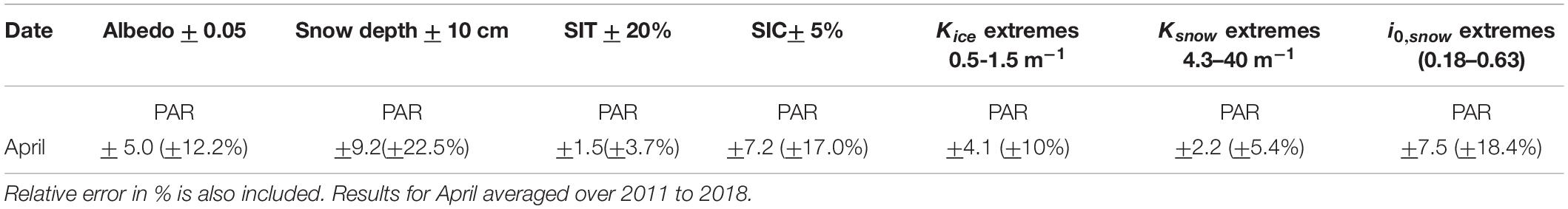
Table 3. Impact of uncertainties in physical sea ice/snow parameters used as input to the Beer–Lambert law on under-ice PAR in μmol m^–2 s^–1.

On the other hand, uncertainties and relative errors for extreme values of the attenuation coefficients have lower overall relative errors compared to snow depth uncertainty, but errors can be as high as 10% for the large range in ice attenuation coefficients used. More important, however, are the large uncertainties in the under-ice PAR as a result of varying the i_o,snow, contributing to an under-ice PAR uncertainty of 7.5 μmol m^–2 s^–1, or relative error of 18.4%. In summary, uncertainties are within 20–30%, which is enough for a qualitative analysis of the pan-Arctic under ice light field, but not for a precise prediction of light levels in specific locations, nor for a precise prediction of timing for the bloom onset. Since the largest uncertainties are associated with snow properties (depth and i_o), this points to snow as the research area where most progress is needed.

Finally, the choice of SIC algorithm used can have a large impact in under-ice light transmission. While Kern et al. (2019) found on a pan-Arctic scale differences between algorithms may cancel out, the NASA Team SIC underestimate those retrieved from visible imagery (e.g., from the NASA Moderate Resolution Imaging Spectroradiometer (MODIS) by 5–10%, whereas SICs from algorithms such as the Bootstrap algorithm (Comiso et al., 1997) overestimate MODIS-derived SICs by a similar amount. Since the Bootstrap algorithm has higher SICs than those from NASA Team, this will reduce the amount of light reaching the ocean surface, especially in the marginal ice zone where the differences between the two algorithms are most pronounced.

Appropriateness of Methodology

In this contribution, we attempt to compute under-ice light levels based on current satellite products, and try to identify uncertainty sources. In this context, the two-level Beer–Lambert approach was the simplest available scheme, which takes into consideration the exponential decay of light through the snow/ice/water media, and gives reasonable transmittance retrievals, as compared with a significant number (N = 234) of data points from the seasonal ice zone (see Figure 1). The setting of AOPs, such as attenuation coefficients, were tuned using field observations over first-year ice, and may not necessarily apply over multiyear ice. However, we found that at least in regards to κ_i, the value obtained of 1 m^–1 differed little from classical multiyear ice derived values (1.5 m^–1). These values are also in line with those of Grenfell and Maykut (1977) (see their Figure 5).

In terms of uncertainties in our under-ice irradiance calculations, the most important uncertainty source relates to non-existent or largely imprecise summer satellite products. In spring, when satellite products are less prone to error, uncertainties are smaller but still within 30% for each of the uncertainty sources. Next to surface albedo, snow in all its aspects appears as a dominant source of uncertainty. This includes the pixel-mean snow depth value, its sub-pixel distribution, and the description of radiative transfer within snow, which is underlined by the large errors on low transmittance values (see Figure 1), and also by the large impact on calculated under-ice PAR of the surface transmission parameter i_o within snow (see Table 3). The new SIT product, derived from ice freeboards processed with the LARM algorithm and using snow data from SnowModel-LG improves the detection limit of CryoSat-2 for thin ice, with a lower freeboard detection limit of ∼2.5 cm (Landy et al., 2020). As evidence for this enhanced thin ice detection, we find that ice thicknesses < 0.5 m make up around 45% of measurements across the October SIT fields, and thicknesses <0.25 m make up around 31% of measurements. While the attenuation coefficients for ice based on first-year ice field data may not be the same as for multiyear ice, uncertainty in k_i played a smaller role than the uncertainty in i_o. These conclusions are in line with those of Katlein et al. (2019), which is based on a different observational dataset and with a slightly different approach.

To improve upon these uncertainties, calculations of under-ice light field would primarily benefit from more precise satellite products, spanning longer periods of the year (discussed further in “Looking to the Future”), in particular regarding ice thickness, snow depth and surface albedo. The sub-pixel distributions of ice characteristics are beyond reach for current observing systems. Yet these can at least be parameterized. For instance, Abraham et al. (2015) provide analytical calculation techniques to account for the sub-pixel snow depth distribution in under-ice light calculations. These can readily be used and at low cost. However, more research is needed to better understand what ice thickness distribution should be used as the ice cover has thinned and transitioned to a first-year ice regime. Generation of open water/leads, melt ponds and thick ice from ridging may differ from earlier studies, and in different regions of the Arctic, which will not only influence the ice thickness distribution, but also snow accumulation. Thus it remains unclear if a pan-Arctic representation of ice thickness and snow depth distribution is applicable as used in this study.

Regarding the formulation of the radiative transfer approach used, an easy recommendation would be to better constrain optical snow parameters from observations over various ice types, based on more observations, more precise, including more snow parameters. Another recommendation would be to use better representations of radiative transfer within snow and ice. Indeed, an easy objection to our methodology is that Beer–Lambert Law is overly simple and does not fully hold in snow, a highly scattering medium (Perovich et al., 2017). Another critique is that the surface scattering layer could be not as well defined in snow as it is in sea ice. While many studies have used the Beer–Lambert Law assuming an exponential attenuation of radiation with length of the medium (e.g., Maykut and Untersteiner, 1971; Bitz and Lipscomb, 1999; Castellani et al., 2017; Vancoppenolle and Tedesco, 2017), more physically elaborated approaches for radiative transfer in snow and ice do exist, in particular two-stream methods, such as such as the delta-Eddington scheme of Briegleb and Light (2007), which relies on the specification of intrinsic optical properties of snow and ice, namely scattering and absorption coefficients. Two-stream schemes have better theoretical foundations and enable the representation of a wider range of optical phenomena (Dang et al., 2019). Yet such schemes are also more complex, more expensive and require information on the vertical profiles of temperature, salinity, density and microstructure (gas, brine, minerals, and grain size), information we do not have from satellites. Hence, at this stage, the use of more elaborated approaches does not warrant lower uncertainties in under-ice light distribution.

Finally, the impact of impurities on transmitted light intensity could also be considered. In particular, ice algae may reduce transmitted light when sufficiently abundant. Here we decided not to take them into account, because we found their effect to be generally low as compared with uncertainties on under-ice transmitted light, and largely uncertain because of unresolved spatio-temporal variations in ice algal content. Significant effects may occur where and when algae are ∼30 mg chl m^–2, and when snow is thin, which may occur in the Bering Sea, or during the season of algal bloom (generally after the month of April). One prerequisite before accounting for ice algae, would be to better constrain their abundance and spatial variability on scales relevant for our study.

Looking to the Future

Massicotte et al. (2019b) show that to properly estimate primary production in the Arctic, we need to assess the spatial variability of sea-ice properties. By under-ice profiling platform (e.g., ROVs and towed nets) we can assess variability on a floe scale, but it is only by means of satellite products that we can provide important information on a pan-Arctic context. This study allows the characterization of the light field over an area large enough to capture the irradiance variability on a pan-Arctic scale. Furthermore, for the first time we are able to provide pan-Arctic maps of under-ice light at a spatial coverage and resolution of most sea-ice numerical models. Most large-scale sea-ice –ocean circulation models adopt the two layers Beer-Lambert approach to describe the radiative transfer, and they employ a SIT and snow depth distribution as in section “Impact of Homogeneous vs. Heterogeneous Snow Depth and Ice Thickness Distributions” to account for sub-grid variability. The present study is a first step in providing products that can be used to directly compare model outputs on a pan-Arctic scale. Moreover, for the first time, we quantify the effects of the sub-grid distribution on the under-ice light levels.

Ideally, we would want to additionally map the under-ice light field from February through October on a pan-Arctic scale, accounting for SIT changes in summer, advanced snow metamorphism, development of melt ponds, and properly account for snow accumulation around ridges. Unfortunately, we lack summer SIT data and melt pond information to extend the characterization of under-ice irradiance beyond April. Temporally, we have been limited by the availability of sea ice freeboard and thickness products. CryoSat-2 provides profiles of SIT observations across the Arctic on a daily basis, but only at the satellite sub-cycle of 30 days does it provide complete pan-Arctic coverage and current algorithms using radar altimetry remain limited to October through April. Since the change from complete darkness to enough sunlight for photosynthesis to occur can happen over a few days, daily coverage is needed. Blending of CryoSat-2 satellite retrievals with Sentinel 3A and 3B, can increase temporal resolution to 10-day frequency (Lawrence et al., 2019). Nevertheless, prior to the melt season, snow depth is arguably more important in limiting light availability and timing of ice algal blooms.

In summer, the most important data gaps to fill are the ice thickness and melt ponds. ICESat-2 offers the ability to provide sea ice freeboards in summer, yet the conversion to total SIT is difficult as this requires information on ice density which is highly variable during the summer melt season. Instead, one could consider using the ICESat-2 freeboards to represent the height of the strongly scattering surface layer (SSL). Typically, the layer has geometric depth 3 – 5 cm and effective scattering about two orders of magnitude larger than the interior ice. The ice between the SSL and sea level (‘drained layer’ DL) also has enhanced light scattering properties, typically one order of magnitude above that of interior ice (see Light et al., 2015, Table 1). Despite their small vertical extent, but because of their strong scattering, these two layers are estimated to have optical depth approximately two orders of magnitude larger than the entire portion of the ice that sits below sea level. Because light penetration will depend most strongly on the portions of the ice with the largest optical depth, it may be possible to estimate transmittance based on the thicknesses of the SSL and DL, as derived directly from summer freeboards. The assumption is that the optical depth of ice above freeboard is about many times more than the optical depth of ice below freeboard, and therefore the amount of ice floating above the water is more important for determining how much light reaches the ocean beneath the ice than the actual SIT.

Once the melt season starts and the snow disappears, melt ponds dominate the amount of light entering the upper ocean beneath the ice. Melt ponds develop in early summer of sizes typically < 10 m, and evolve into a temporally and spatially heterogeneous network of melt ponds intermixed by bare ice and snow-covered ice regions. While melt ponds are not difficult to detect using high resolution satellite imagery, such as that from meter-scale WorldView optical imagery (e.g., Wright and Polashenski, 2018), pan-Arctic coverage and long time-series are not available from such high resolution imagery. Instead, moderate resolution satellite sensors, such as the NASA Moderate Resolution Imaging Spectroradiometer (MODIS) satellite have been used to map melt ponds at a pan-Arctic scale (e.g., Rösel and Kaleschke, 2012). MODIS has a spatial resolution of 250 m for the first two visible channels and 500 m for the other five visible channels. Since the melt ponds have a relatively small size in relationship to the large footprint of the satellite image, several ice types are present within each satellite pixel, requiring some sort of spectral unmixing to retrieve the melt pond fraction. Spectral mixture analysis (SMA) (e.g., Tschudi et al., 2008; Rösel and Kaleschke, 2012) and Multiple Endmember Spectral Mixture Analysis (MESMA) (e.g., Yackel et al., 2018) have been used with limited success to map sub-pixel fractional area of surface types, yet reference spectra for ice types can vary considerably and cause large errors in melt pond fraction retrievals. Currently there are no up-to-date pan-Arctic melt pond products being provided by the science community.

Similarly, as the ice cover has transitioned from one dominated by multiyear ice year-round to one dominated by first-year ice, the dynamics of the ice cover have increased, creating more occurrence of ice fracture and lead formation (e.g., Rampal et al., 2009). Leads result in new ice formation, and thus thin ice with little to no snow cover, and thus play an important role in light transmission before the melt season starts. Evidence from an Arctic fjord found that 77–86% of incidence light from 0.4 to 0.7 μm was transmitted through leads (Taskjelle et al., 2016). Changes in albedo may in part reflect increased fracturing, leads and thin ice formation. On the other hand, evaluation of the APP-X data set shows non-physical artifacts in albedo that have an impact on the under-ice PAR calculations, and more improvements are needed to develop a long-term and reliable surface albedo product.

Finally, ridges play an important role in redistributing snow accumulation. While several approaches exist to quantify surface roughness from satellite, including laser altimetry (e.g., Landy et al., 2015; Petty et al., 2016), multi-angular optical imagery (e.g., Nolin and Mar, 2019), and SAR backscatter (e.g., Fors et al., 2016), the small footprint of the ICESat-2 ATLAS photon-counting instrument (∼15 m), together with dense along-track spacing (∼70 cm) and precise elevation measurements (<10 cm) will allow for mapping of ridge heights. This is because ICESat-2 will provide consecutive elevation measurements to define the ridge height and edges with sufficient precision. This information could be used in conjunction with SnowModel to map snow depth at high spatial resolution and then downscale to the pan-Arctic scale.

Conclusion

Arctic marine ecosystems have adapted to extremes in light conditions, taking advantage of the short time-period over which primary production can occur. Since satellites sensors cannot ‘see through’ the sea ice, the response of Arctic primary production to changes in sea ice and snow properties can only be determined with continuous in situ monitoring of algae and phytoplankton stocks, together with the main physical drivers affecting their phenology: under-ice light field, sea ice and snow properties, temperature and salinity of the ocean surface, nutrients and mixed layer depth. However, the lack of long-term data covering different regions and seasons makes this challenging at present. In this paper we have attempted to map one component important for ocean primary production, the light under the ice on a pan-Arctic scale using currently available satellite-based products on snow and ice conditions together with parameterizations established from cruises and other in situ observations. Our estimates of under-ice PAR are based on the Beer–Lambert Law, and our interactions of light with snow and ice are based on empirical parameterizations from in situ data collections that depend at the moment solely on the ice thickness and snow depth, whether or not the snowpack is melting, as well as the surface albedo. Key uncertainties in our under-ice PAR calculations relate to how precise current parameterizations are, how best to distribute the mean snow and ice thickness within a 25-km grid scale, as well as errors in satellite-retrieved variables of surface albedo, ice thickness and concentration, and how best to model snow accumulation.

During springtime, the high albedo of snow and its capacity to attenuate solar radiation means that snow depth variability largely controls under-ice PAR variability from year-to year, with some years showing increased light penetration especially in the Beaufort Sea in April. During October, ice thickness, albedo and lead fraction play a more important role as there is little snow on the ice. Ice algal in particular have adapted to very low light levels (e.g., Berge et al., 2015), with the first bloom happening in the bottom layer of the sea ice already in spring when light for photosynthesis becomes available. Thus, despite little light entering the Arctic Ocean in February and March, inter-annual snow depth variability can lead to more light availability even during these months that is enough to initiate algal growth, whereas long-term declines in snow depth over time may be shifting the timing of under ice algal blooms to earlier in the year. This has important implications on marine ecosystems, as ice algae are an early food source for certain pelagic grazers (e.g., Leu et al., 2015).

New satellite sensors, such as ICESat-2, could enable these under-ice maps to be extended to be year round, whilst on-going in situ field programs, such as EcoLight and MOSAiC, will allow us to refine the algorithms and more accurately predict light penetration through a range of snow and ice conditions. While there are significant challenges to overcome before we routinely produce daily pan-Arctic under-ice light maps using satellite observations, we feel new satellite-derived products and focused in situ campaigns are closing the gap.

Data Availability Statement

The datasets presented in this study can be found in online repositories. The names of the repository/repositories and accession number(s) can be found below: ftp://sidads.colorado.edu/pub/projects/SIPN/Ecolight. All AVHRR Polar Pathfinder albedo and incoming solar radiation data are available from NOAA National Centers for Environmental Information (https://www.ncdc.noaa.gov/cdr/atmospheric/extended-avhrr-polar-pathfinder-app-x). Sea ice concentration data is available from the National Snow and Ice Data Center Sea Ice Index (https://nsidc.org/data/seaice_index).

Author Contributions

JS wrote the manuscript. GV and MV produced the figures. All the authors edited the manuscript.

Funding

This work resulted from the NERC project (NE/R012725/1), known as EcoLight, part of the Changing Arctic Ocean programme, jointly funded by the UKRI Natural Environment Research Council (NERC) and the German Federal Ministry of Education and Research (BMBF). JS and GL were also funded under NASA NNX16AK85G. JL was funded under NERC Diatom-ARCTIC (NE/R012849/1). JS was also partially funded under the Canada 150 Chair Program and NASA Grant 80NSSC20K1121.

Conflict of Interest

MK was employed by O.A.Sys-Ocean Atmosphere Systems GmbH.

The remaining authors declare that the research was conducted in the absence of any commercial or financial relationships that could be construed as a potential conflict of interest.

Footnotes

1. ^ https://doi.pangaea.de/10.1594/PANGAEA.902056

References

Abraham, C., Steiner, N., Monahan, A., and Michel, C. (2015). Effects of subgrid-scale snow thickness variability on radiative transfer in sea ice. J. Geophys. Res. Oceans 120, 5597–5614. doi: 10.1002/2015JC010741

CrossRef Full Text | Google Scholar

Ardyna, M., Babin, B., Gosselin, M., Devred, E., Rainville, L., and Tremblay, J.-E. (2014). Recent Arctic Ocean sea ice loss triggers novel fall phytoplankton blooms. Geophys. Res. Lett. 41, 6207–6212. doi: 10.1002/2014GL061047

CrossRef Full Text | Google Scholar

Arrigo, K. R., and van Dijken, G. L. (2011). Secular trends in Arctic Ocean net primary production. J. Geophys. Res. 116:C09011. doi: 10.1029/2011JC007151

CrossRef Full Text | Google Scholar

Assmy, P., Fernández-Méndez, M., Duarte, P., Meyer, A., Randelhoff, A., Mundy, C. J., et al. (2017). Leads in Arctic pack ice enable early phytoplankton blooms below snow-covered sea ice. Sci. Rep. 7:40850. doi: 10.1038/srep40850

PubMed Abstract | CrossRef Full Text | Google Scholar

Barrett, A. P., Stroeve, J., and Serreze, M. C. (2019). Arctic Ocean precipitation from atmospheric reanalysis and comparisons with north pole drifting station records. J. Geophys. Res. Oceans 125:e2019JC015415.

Google Scholar

Berge, J., Cottier, F., Varpe, O., Renaud, P. E., Falk-Petersen, S., Kwasniewski, S., et al. (2014). Arctic complexity: a case study on diel vertical migration of zooplankton. J. Plankton Res. 36, 1279–1297. doi: 10.1093/plankt/fbu059

PubMed Abstract | CrossRef Full Text | Google Scholar

Berge, J., Renaud, P. E., Darnis, G., Cottier, F., Last, K., Gabrielsen, T. M., et al. (2015). In the dark: a review of ecosystem processes during the Arctic polar night. Prog. Oceanogr. 139, 258–271. doi: 10.1016/j.pocean.2015.08.005

CrossRef Full Text | Google Scholar

Bitz, C. M., and Lipscomb, W. H. (1999). An energy-conserving thermodynamic model of sea ice. J. Geophys. Res. 104, 15669–15677. doi: 10.1029/1999JC900100

CrossRef Full Text | Google Scholar

Blanchard-Wrigglesworth, E., Webster, M., Farrell, S., and Bitz, C. M. (2018). Reconstruction of Arctic snow on sea ice. J. Geophys. Res. Oceans 123, 3588–3602.

Google Scholar

Bluhm, B. A., Swadling, K. M., and Gradinger, R. (2017). “Chapter 16: Sea ice as a habitat for macrograzers,” in Sea Ice, ed. D. N. Thomas (Chichester: John Wiley & Sons Ltd), 394–414. doi: 10.1002/9781118778371.ch16

CrossRef Full Text | Google Scholar

Briegleb, B. P., and Light, B. (2007). A Delta-Eddington Multiple Scattering Parameterization for Solar Radiation in the Sea Ice Component of the Community Climate System Model, National Center for Atmospheric Research Technical Note No. NCAR/TN-472+STR. Boulder, CO: National Center for Atmospheric Research, 100.

Google Scholar

Castellani, G., Losch, M., Lange, B. A., and Flores, H. (2017). Modeling Arctic sea-ice algae: physical drivers of spatial distribution and algae phenology. J. Geophys. Res. Oceans 122, 7466–7487. doi: 10.1002/2017JC012828

CrossRef Full Text | Google Scholar

Castellani, G., Schaafsma, F. L., Arndt, S., Lange, B. A., Peeken, I., Ehrlich, J., et al. (2020). Large-Scale Variability of Physical and Biological Sea-Ice Properties in Polar Oceans. Front. Mar. Sci. 7:536 doi: 10.3389/fmars.2020.00536

CrossRef Full Text | Google Scholar

Castro-Morales, K., Kauker, F., Losch, M., Hendricks, S., Riemann-Campe, K., and Gerdes, R. (2014). Sensitivity of simulated Arctic sea ice to realistic ice thickness distributions and snow parameterizations. J. Geophys. Res. Oceans 119, 559–571. doi: 10.1002/2013jc009342

CrossRef Full Text | Google Scholar

Cavalieri, D. J., Parkinson, C. L., Gloersen, P., and Zwally, H. J. (1997). Arctic and Antarctic Sea Ice Concentrations from Multichannel Passive-Microwave Satellite Data Sets: October 1978-September 1995 – User’s Guide. NASA TM 104647. Greenbelt, MD: Goddard Space Flight Center, 17.

Google Scholar

Comiso, J. C., Cavalieri, D., Parkinson, C., and Gloersen, P. (1997). Passive microwave algorithms for sea ice concentrations: a comparison of two techniques. Rem. Sens. Environ. 60, 357–384. doi: 10.1016/s0034-4257(96)00220-9

CrossRef Full Text | Google Scholar

Comiso, J. C., Cavalieri, D. J., and Markus, T. (2003). Sea ice concentration, ice temperature, and snow depth using AMSR-E data. IEEE Trans. Geosci. Rem. Sens. 41, 243–252. doi: 10.1109/tgrs.2002.808317

CrossRef Full Text | Google Scholar

Dang, C., Zender, C. S., and Flanner, M. G. (2019). Intercomparison and improvement of two-stream shortwave radiative transfer schemes in Earth system models for a unified treatment of cryospheric surfaces. Cryosphere 13, 2325–2343. doi: 10.5194/tc-13-2325-2019

CrossRef Full Text | Google Scholar

Durant, J. M., Hjermann, D. Ø, Ottersen, G., and Stenseth, N. C. (2007). Climate and the match or mismatch between predator requirements and resource availability. Clim. Res. 33, 271–283. doi: 10.3354/cr033271

CrossRef Full Text | Google Scholar

Eicken, H., Shapiro, L., Gaylord, A., Mahoney, A., and Cotter, P. (2006). Mapping and Characterization of Recurring Spring Leads and Landfast Ice in the Beaufort and Chukchi Seas, Final Report, Minerals Management Service OCS Study MMS 2005-068. Anchorage, AK: U.S. Dept. of the Interior, 180.

Google Scholar

Fernández-Méndez, M., Olsen, L. M., Kauku, H. M., Meyer, A., Rösel, A., Merkouriadi, I., et al. (2018). Algal hot spots in a changing Arctic Ocean: sea-ice ridges and the snow-ice interface. Front. Mar. Sci. 5:75. doi: 10.3389/fmars.2018.00075

CrossRef Full Text | Google Scholar

Fetterer, F., Knowles, K., Meier, W. N., Savoie, M., and Windnagel, A. K. (2017). Updated Daily. Sea Ice Index, Version 3. [Indicate subset used]. Boulder, CO: NSIDC: National Snow and Ice Data Center. doi: 10.7265/N5K072F8

CrossRef Full Text | Google Scholar

Fichefet, T., and Morales Maqueda, M. A. (1997). Sensitivity of a global sea ice model to the treatment of ice thermodynamics and dynamics. J. Geophys. Res. 102, 12609–12646. doi: 10.1029/97JC00480

CrossRef Full Text | Google Scholar

Fors, A. S., Brekke, C., Gerland, S., Doulgeris, A. P., and Beckers, J. F. (2016). Late summer Arctic sea ice surface roughness signatures in C-band SAR data. IEEE J. Sel. Top. Appl. Earth Obs. Rem. Sens. 9, 1199–1215. doi: 10.1109/JSTARS.2015.2504384

CrossRef Full Text | Google Scholar

Frey, K. E., Perovich, D. K., and Light, B. (2011). The spatial distribution of solar radiation under a melting Arctic sea ice cover. Geophys. Res. Lett. 38:L22501. doi: 10.1029/2011GL04942

CrossRef Full Text | Google Scholar

Frouin, R., and Murakami, H. J. (2007). Estimating photosynthetically available radiation at the ocean surface from ADEOS-II global imager data. J. Oceanogr. 63, 493–503. doi: 10.1007/s10872-007-0044-3

CrossRef Full Text | Google Scholar

Frouin, R., and Pinker, R. T. (1995). Estimating photosynthetically active radiation (PAR) at the earth’s surface from satellite observations. Rem. Sen. Environ. 51, 98–107. doi: 10.1016/0034-4257(94)00068-x

CrossRef Full Text | Google Scholar

Gelaro, R., McCarty, W., Suárez, M. J., Todling, R., Molod, A., Takacs, L., et al. (2017). The modern-era retrospective analysis for research and applications, version 2 (MERRA-2). J. Clim. 30, 5419–5454. doi: 10.1175/JCLI-D-16-0758.1

PubMed Abstract | CrossRef Full Text | Google Scholar

Goosse, H., Arzel, O., Bitz, C. M., de Montety, A., and Vancoppenolle, M. (2009). Increased variability of the Arctic summer ice extent in a warmer climate. Geophys. Res. Lett. 36:L23702. doi: 10.1029/2009GL040546

CrossRef Full Text | Google Scholar

Grenfell, T. C., and Maykut, G. A. (1977). The optical properties of ice and snow in the Arctic Basin. J. Glaciol. 18, 445–463. doi: 10.1017/s0022143000021122

CrossRef Full Text | Google Scholar

Grenfell, T. C., and Perovich, D. K. (2008). Incident spectral irradiance in the Arctic Basin during the summer and fall. J. Geophys. Res. 113:D12117. doi: 10.1029/2007JD009418

CrossRef Full Text | Google Scholar

Haas, C., Hendricks, S., Eicken, H., and Herber, A. (2010). Synoptic airborne thickness surveys reveal state of Arctic sea ice cover. Geophys. Res. Lett. 37:L09501. doi: 10.1029/2010GL042652

CrossRef Full Text | Google Scholar

Hancke, K., Lund-Hansen, L. C., Lamare, M. L., Pedersen, S. H., King, M. D., Andersen, P., et al. (2018). Extreme low light requirement for algae growth underneath sea ice: a case study from Station Nord, NE Greenland. J. Geophys. Res. Oceans 123, 985–1000. doi: 10.1002/2017JC013263

CrossRef Full Text | Google Scholar

Hendricks, S., Ricker, R., and Helm, V. (2016). User Guide – AWI CryoSat-2 Sea Ice Thickness Data Product (v1.2). hdl:10013/epic.48201. Cary, NC: EPIC

Google Scholar

Hibler, W. D. (1984). “The role of sea ice dynamics in modelling CO2 increases,” in Climate Processes and Climate Sensitivity, eds J. E. Hansen and T. Takahashi (Washington, DC: AGU), 238–253. doi: 10.1029/gm029p0238

CrossRef Full Text | Google Scholar

Horner, R. A., and Schrader, G. C. (1982). Relative contributions of ice algae, phytoplankton, and benthic microalgae to primary production in nearshore regions of the Beaufort Sea. ARCTIC 35, 485–503.

Google Scholar

Horvat, C., Jones, D. R., Iams, S., Schroeder, D., Flocco, D., and Feltham, D. (2017). The frequency and extent of sub-ice phytoplankton blooms in the Arctic Ocean. Sci. Adv. 3:e1601191. doi: 10.1126/sciadv.1601191

PubMed Abstract | CrossRef Full Text | Google Scholar

Huang, Y., Dong, X., Bailey, D. A., Holland, M. M., Xi, B., DuVivier, A. K., et al. (2019). Thicker clouds and accelerated Arctic sea ice decline: the atmosphere-sea ice interactions in spring. Geophys. Res. Lett. 46, 6980–6989. doi: 10.1029/2019GL082791

CrossRef Full Text | Google Scholar

Ivanova, N., Pedersen, L. T., Tonboe, R. T., Kern, S., Heygster, G., Lavergne, T., et al. (2015). Inter-comparison and evaluation of sea ice algorithms: towards further identification of challenges and optimal approach using passive microwave observations. Cryosphere 9, 1797–1817. doi: 10.5194/tc-9-1797-2015

CrossRef Full Text | Google Scholar

Järvinen, O., and Leppäranta, M. (2011). Transmission of solar radiation through the snow cover on floating ice. J. Glaciol. 57, 861–870. doi: 10.3189/002214311798043843

CrossRef Full Text | Google Scholar

Katlein, C., Arndt, S., Belter, H. J., Castellani, G., and Nicolaus, M. (2019). Seasonal evolution of light transmission distributions through Arctic sea ice. J. Geophys. Res. Oceans 124, 5418–5435. doi: 10.1029/2018JC014833

CrossRef Full Text | Google Scholar

Kern, S., Lavergne, T., Notz, D., Pedersen, L. T., Tonboe, R. T., Saldo, R., et al. (2019). Satellite passive microwave sea-ice concentration data set intercomparison: closed ice and ship-based observations. Cryosphere 13, 3261–3307. doi: 10.5194/tc-13-3261-2019

CrossRef Full Text | Google Scholar

Key, J., Liu, Y., Wang, X., and Program, N. O. A. A. C. D. R. (2019). NOAA Climate Data Record (CDR) of AVHRR Polar Pathfinder (APP) Cryosphere, Version 2.0. Boulder, CO: NOAA National Centers for Environnemental Information (NCEI). doi: 10.25921/X2X1-JR34

CrossRef Full Text | Google Scholar

Key, J., Schweiger, A. J., and Stone, R. S. (1997). Expected uncertainty in satellite-derived estimates of the high-latitude surface radiation budget. J. Geophys. Res. 102, 15837–15847. doi: 10.1029/97jc00478

CrossRef Full Text | Google Scholar

Kohlbach, D., Graeve, M., Lange, B. A., David, C., Peeken, I., and Flores, H. (2016). The importance of ice algae-produced carbon in the central Arctic Ocean ecosystem: food web relationships revealed by lipid and stable isotope analyses. Limnol. Oceanogr. 61, 2027–2044. doi: 10.1002/lno.10351

CrossRef Full Text | Google Scholar

Kohlbach, D., Shaafsma, F. L., Graeve, M., Lebreton, B., Lange, B. A., David, C., et al. (2017). Strong linkage of polar cod (Boreogadus saida) to sea ice algae-produced carbon: evidence from stomach content, fatty acid and stable isotope analyses. Progr. Oceanogr. 152, 62–74. doi: 10.1016/j.pocean.2017.02.003

CrossRef Full Text | Google Scholar

Kurtz, N., and Harbeck, J. (2017). CryoSat-2 Level-4 Sea Ice Elevation, Freeboard, and Thickness, Version 1. Boulder, CO: NASA National Snow and Ice Data Center Distributed Active Archive Center. doi: 10.5067/96JO0KIFDAS8

CrossRef Full Text | Google Scholar

Kurtz, N. T., Galin, N., and Studinger, M. (2014). An improved CryoSat-2 sea ice freeboard retrieval algorithm through the use of a waveform fitting. Cryosphere 8, 1217–1237. doi: 10.5194/tc-802017-2014

CrossRef Full Text | Google Scholar

Kwok, R., and Cunningham, G. F. (2008). ICESat over Arctic sea ice: estimation of snow depth and ice thickness. J. Geophys. Res. 113:C08010. doi: 10.1029/2008JC004753

CrossRef Full Text | Google Scholar

Kwok, R., and Markus, T. (2018). Potential basin-scale estimates of Arctic snow depth with sea ice freeboards from CryoSat-2 and ICESat-2: an exploratory analysis. Adv. Space Res. 62, 1243–1250. doi: 10.1016/j.asr.2017.09.007

CrossRef Full Text | Google Scholar

Landy, J. C., Ehn, J. K., and Barber, D. G. (2015). Albedo feedback enhanced by smoother Arctic sea ice. Geophys. Res. Lett. 42, 10714–10720.

Google Scholar

Landy, J. C., Petty, A. A., Tsamados, M., and Stroeve, J. C. (2020). Sea ice roughness overlooked as a key source of uncertainty in CryoSat-2 ice freeboard retrievals. J. Geophys. Res. Oceans 125, e2019JC015820.

Google Scholar

Landy, J. C., Tsamados, M., and Scharien, R. K. (2019). A facet-based numerical model for simulating SAR altimeter echoes from heterogeneous sea ice surfaces. IEEE Trans. Geosci. Rem. Sens. 57, 4164–4180. doi: 10.1109/TGRS.2018.2889763

CrossRef Full Text | Google Scholar

Lawrence, I. R., Armitage, T. W. K., Tsamados, M. C., Stroeve, J. C., Dinardo, S., Ridout, A. L., et al. (2019). Extending the Arctic sea ice freeboard and sea level record with the Sentinel-3 radar altimeters. Adv. Space Res. doi: 10.1016/j.asr.2019.10.011

CrossRef Full Text | Google Scholar

Lawrence, I. R., Tsamados, M. C., Stroeve, J. C., Armitage, T. W. K., and Ridout, A. L. (2018). Estimating snow depth over Arctic sea ice from calibrated dual-frequency radar freeboards. Cryosphere 12, 3551–3564. doi: 10.5194/tc-12-3551-2018

CrossRef Full Text | Google Scholar

Laxon, S. W., Giles, K. A., Ridout, A. L., Wingham, D. J., Willatt, R., Cullen, R., et al. (2013). CryoSat-2 estimates of Arctic sea ice thickness and volume. Geophys. Res. Lett. 40, 732–737. doi: 10.1002/grl.50193

CrossRef Full Text | Google Scholar

Lebrun, M. (2019). De L’interaction Entre Banquise, Lumière et Phytoplancton Arctique. Ph.D thesis, Sorbonne Université, Paris.

Google Scholar

Lee, S., Im, J., Kim, J., Kim, M., Shin, M., Kim, H.-C., et al. (2016). Arctic sea ice thickness estimation from CryoSat-2 satellite data using machine learning-based lead detection. Rem. Sens. 8:698. doi: 10.3390/rs8090698

CrossRef Full Text | Google Scholar

Letelier, R. M., Karl, D. M., Abbott, M. R., and Bidigare, R. R. (2004). Light driven seasonal patterns of chlorophyll and nitrate in the lower euphotic zone of the North Pacific Subtropical Gyre. Limnol. Oceanogr. 49, 508–519. doi: 10.4319/lo.2004.49.2.0508

CrossRef Full Text | Google Scholar

Leu, E., Mundy, C. J., Assmy, P., Campbell, K., Gabrielsen, T. M., Gosselin, M., et al. (2015). Arctic spring awakening – steering principles behind the phenology of vernal ice algal blooms. Prog. Oceanogr. 139, 151–170. doi: 10.1016/j.pocean.2015.07.012

CrossRef Full Text | Google Scholar

Lewis, B. J., and Hutchings, J. K. (2019). Leads and associated sea ice drift in the Beaufort Sea in winter. J. Geophys. Res. Oceans 124, 3411–3427. doi: 10.1029/2018JC014898

CrossRef Full Text | Google Scholar

Light, B., Grenfell, T. C., and Perovich, D. K. (2008). Transmission and absorption of solar radiation by Arctic sea ice during the melt season. J. Geophys. Res. 113:C03023. doi: 10.1029/2006JC003977

CrossRef Full Text | Google Scholar

Light, B., Perovich, D. K., Webster, M. A., Polashenski, C., and Dadic, R. (2015). Optical properties of melting first-year Arctic sea ice. J. Geophys. Res. Oceans 120, 7657–7675. doi: 10.1002/2015JC011163

CrossRef Full Text | Google Scholar

Lindsay, R., and Schweiger, A. (2015). Arctic sea ice thickness loss determined using subsurface, aircraft, and satellite observations. Cryosphere 9, 269–283. doi: 10.5194/tc-9-269-2015

CrossRef Full Text | Google Scholar

Liston, G. E. (1995). Local advection of momentum, heat, and moisture during the melt of patchy snow covers. J. Appl. Meteorol. 34, 1705–1715. doi: 10.1175/1520-0450-34.7.1705

CrossRef Full Text | Google Scholar

Liston, G. E., Haehnel, R. B., Sturm, M., Hiemstra, C. A., Berezovskaya, S., and Tabler, R. D. (2007). Simulating complex snow distributions in windy environments using SnowTran-3D. J. Glaciol. 53, 241–256. doi: 10.3189/172756507782202865

CrossRef Full Text | Google Scholar

Liston, G. E., and Hall, D. K. (1995). An energy balance model of lake ice evolution. J. Glaciol. 41, 373–382. doi: 10.1017/s0022143000016245

CrossRef Full Text | Google Scholar

Liston, G. E., Itkin, P., Stroeve, J., Tschudi, M., and Stewart, J. S. (2020). A lagrangian snow-evolution system for sea-ice applications (SnowModel-LG): Part I - Model description. J. Geophys. Res. Oceans 125:e2019JC015913. doi: 10.1029/2019jc015913

PubMed Abstract | CrossRef Full Text | Google Scholar

Liston, G. E., and Mernild, S. H. (2012). Greenland freshwater runoff. Part I: A runoff routing model for glaciated and non-glaciated landscapes (HydroFlow). J. Clim. 25, 5997–6014. doi: 10.1175/jcli-d-11-00591.1

CrossRef Full Text | Google Scholar

Liston, G. E., Polashenski, C., Roesel, A., Itkin, P., King, J., Merkouriadi, I., et al. (2018). A distributed snow-evolution model for sea-ice applications (SnowModel). J. Geophys. Res. Oceans 123, 3786–3810. doi: 10.1002/1027/JC013706

CrossRef Full Text | Google Scholar

Liston, G. E., and Sturm, M. (1998). A snow-transport model for complex terrain. J. Glaciol. 44, 498–516. doi: 10.3189/s0022143000002021

CrossRef Full Text | Google Scholar

Liston, G. E., Winther, J.-G., Bruland, O., Elvehøy, H., and Sand, K. (1999). Below-surface ice melt on the coastal Antarctic ice sheet. J. Glaciol. 45, 273–285. doi: 10.3189/S0022143000001775

CrossRef Full Text | Google Scholar

Markus, T., and Cavalieri, D. J. (1998). “Snow depth distribution over sea ice in the Southern Ocean from satellite passive microwave data,” in Antarctic Sea Ice Physical Processes, Interactions and Variability, Antarctic Research Series, Vol. 74, ed. M. O. Jeffries (Washington, DC: AGU), 19–40. doi: 10.1029/ar074p0019

CrossRef Full Text | Google Scholar

Markus, T., Stroeve, J. C., and Miller, J. (2009). Recent changes in Arctic sea ice melt onset, freezeup, and melt season length. J. Geophys. Res. 114:C12024. doi: 10.1029/2009JC005436

CrossRef Full Text | Google Scholar

Maslanik, J., Stroeve, J., Fowler, C., and Emery, W. (2011). Distribution and trends in Arctic sea ice age through spring 2011. Geophys. Res. Lett. 38:L13502. doi: 10.1029/2011GL047735

CrossRef Full Text | Google Scholar

Massicotte, P., Peeken, I., Katlein, C., Flores, H., Huot, Y., Castellani, G., et al. (2019a). Sensitivity of phytoplankton primary production estimates to available irradiance under heterogeneous sea ice conditions. J. Geophys. Res.: Oceans, 124, 5436–5450. doi: 10.1029/2019JC015007

CrossRef Full Text | Google Scholar

Massicotte, P., Peeken, I., Katlein, C., Flores, H., Huot, Y., Castellani, G., et al. (2019b). Sensitivity of phytoplankton primary production estimates to available irradiance under heterogeneous sea ice conditions. J. Geophys. Res. Oceans 124, 5436–5450. doi: 10.1029/2019JC015007

CrossRef Full Text | Google Scholar

Maykut, G. A. (1986). “The surface heat and mass balance,” in The Geophysics of Sea Ice. NATO ASI Series (Series B: Physics), ed. N. Untersteiner (Boston, MA: Springer).

Google Scholar

Maykut, G. A., and McPhee, M. G. (1995). Solar heating of the Arctic mixed layer. J. Geophys. Res. 100, 24691–24703. doi: 10.1029/95jc02554

CrossRef Full Text | Google Scholar

Maykut, G. A., and Untersteiner, N. (1971). Some results from a time-dependent thermodynamic model of sea ice. J. Geophys. Res. 76, 1550–1575. doi: 10.1029/JC076i006p01550

CrossRef Full Text | Google Scholar

Mock, T., and Gradinger, R. (1999). Determination of Arctic ice algal production with a new in situ incubation technique. Mar. Ecol. Prog. Ser. 177, 15–26. doi: 10.3354/meps177015

CrossRef Full Text | Google Scholar

Morel, A., and Smith, R. C. (1974). Relation between total quanta and total energy for aquatic photosynthesis. Limnol. Oceanogr. 19, 591–600. doi: 10.4319/lo.1974.19.4.0591

CrossRef Full Text | Google Scholar

Moritz, R. E., Curry, J. A., Thorndike, A. S., and Untersteiner, N. (1993). SHEBA, a research program on the surface heat budget of the Arctic Ocean. Arct. Syst. Sci. Rep. 3:34.

Google Scholar

Mundy, C. J., Barber, D. G., and Michel, C. (2005). Variability of snow and ice thermal, physical and optical properties pertinent to sea ice algae biomass during spring. J. Mar. Syst. 58, 107–120. doi: 10.1016/j.jmarsys.2005.07.003

CrossRef Full Text | Google Scholar

Nicolaus, M., Katlein, C., Maslanik, J., and Hendricks, S. (2012). Changes in Arctic sea ice result in increasing light transmittance and absorption. Geophy. Res. Lett. 39:L24501. doi: 10.1029/2012GL053738

CrossRef Full Text | Google Scholar

Nolin, A. W., and Mar, E. (2019). Arctic sea ice surface roughness estimated from multi-angular reflectance satellite imagery. Remote Sens. 11:50. doi: 10.3390/rs11010050

CrossRef Full Text | Google Scholar

Oziel, L., Massicotte, P., Randelhoff, A., Ferland, J., Vladoiu, A., Lacour, L., et al. (2019). Environmental factors influencing the seasonal dynamics of under-ice spring blooms in Baffin Bay. Elem. Sci. Anth. 7:34.

Google Scholar

Pegau, W., and Paulson, C. (2001). The albedo of Arctic leads in summer. Ann. Glaciol. 33, 221–224. doi: 10.3189/172756401781818833

CrossRef Full Text | Google Scholar

Perovich, D., Polashenski, C., Arntsen, A., and Stwertka, C. (2017). Anatomy of a late spring snowfall on sea ice. Geophys. Res. Lett. 44, 2802–2809. doi: 10.1002/2016GL071470

CrossRef Full Text | Google Scholar

Perovich, D. K., and Gow, A. J. (1996). A quantitative description of sea ice inclusions. J. Geophys. Res. 101, 18327–18343. doi: 10.1029/96JC01688

CrossRef Full Text | Google Scholar

Perovich, D. K., Grenfell, T. C., Light, B., and Hobbs, P. V. (2002). Seasonal evolution of the albedo of multiyear Arctic sea ice. J. Geophys. Res. 107:8044. doi: 10.1029/2000JC000438

CrossRef Full Text | Google Scholar

Perovich, D. K., Light, B., Eicken, H., Jones, K. F., Runciman, K., and Nghiem, S. V. (2007). Increasing solar heating of the Arctic Ocean and adjacent seas, 1979–2005: attribution and role in the ice-albedo feedback. Geophys. Res. Lett. 34:L19505. doi: 10.1029/2007GL031480

CrossRef Full Text | Google Scholar

Petty, A. A., Tsamados, M. C., Kurtz, N. T., Farrell, S. L., Newman, T., Harbeck, J. P., et al. (2016). Characterizing Arctic sea ice topography using high-resolution IceBridge data. Cryosphere 10, 1161–1179. doi: 10.5194/tc-10-1161-2016

CrossRef Full Text | Google Scholar

Petty, A. A., Webster, M., Boisvert, L. N., and Markus, T. (2018). The NASA Eulerian snow on sea ice model (NESOSIM) v1.0: initial model development and analysis. Geosci. Model Dev. 11, 4577–4602. doi: 10.5194/gmd-11-4577-2018

CrossRef Full Text | Google Scholar

Popova, E. E., Yool, A., Coward, A. C., Aksenov, Y. K., Alderson, S. G., de Cuevas, B. A., et al. (2010). Control of primary production in the Arctic by nutrients and light: insights from a high resolution ocean general circulation model. Biogeosciences 7, 3569–3591. doi: 10.5194/bg-7-3569-2010

CrossRef Full Text | Google Scholar

Rampal, P., Weiss, J., and Marsan, D. (2009). Positive trend in the mean speed and deformation rate of Arctic sea ice, 1979–2007. J. Geophys. Res. Oceans 114, c05013. doi: 10.1029/2008JC005066

CrossRef Full Text | Google Scholar

Randelhoff, A., Holding, J., Janout, M., Sejr, M. K., Babin, M., Tremblay, J.-E., et al. (2020). Pan-Arctic Ocean primary production constrained by turbulent nitrate fluxes. Front. Mar. Sci. 7:150. doi: 10.3389/fmars.2020.00150

CrossRef Full Text | Google Scholar

Randelhoff, A., Oziel, L., Massicotte, P., Bécu, G., Galí, M., Lacour, L., et al. (2019). The evolution of light and vertical mixing across a phytoplankton ice-edge bloom. Elem. Sci. Anth. 7:20. doi: 10.1525/elementa.357

PubMed Abstract | CrossRef Full Text | Google Scholar

Renner, A. H. H., Hendricks, S., Gerland, S., Beckers, J., Haas, C., and Krumpen, T. (2013). Large-scale ice thickness distribution of first-year sea ice in spring and summer north of Svalbard. Ann. Glaciol. 54, 13–18. doi: 10.3189/2013AoG62A146

CrossRef Full Text | Google Scholar

Ricker, R., Hendricks, S., Kaleschke, L., Tian-Kunze, X., King, J., and Haas, C. (2017). A weekly Arctic sea-ice thickness data record from merged CryoSat-2 and SMOS satellite data. Cryosphere 11, 1607–1623. doi: 10.5194/tc-11-1607-2017

CrossRef Full Text | Google Scholar

Rösel, J., and Kaleschke, L. (2012). An algorithm to detect sea ice leads by using AMSR-E passive microwave imagery. Cryosphere 6, 343–352. doi: 10.5194/tc-6-343-2012

CrossRef Full Text | Google Scholar

Scharien, R. K., Segal, R., Nasonova, S., Nandan, V., Howell, S. E. L., and Haas, C. (2017). Winter Sentinel-1 backscatter as a predictor of spring Arctic sea ice melt pond fraction. Geophys. Res. Lett. 44, 12262–12270. doi: 10.1002/2017GL075547

CrossRef Full Text | Google Scholar

Stroeve, J., Liston, G. E., Buzzard, S., Zhou, L., Mallett, R., Barrett, A., et al. (2020). A Lagrangian snow-evolution system for sea-ice applications (SnowModel-LG): Part II – Analyses. J. Geophys. Res. Oceans 125:e2019JC015900. doi: 10.1029/2019jc015900

CrossRef Full Text | Google Scholar

Stroeve, J., and Notz, D. (2018). Changing state of Arctic sea ice across all seasons. Env. Res. Lett. 13:103001. doi: 10.1088/1748-9326/aade.56

CrossRef Full Text | Google Scholar

Stroeve, J. C., Markus, T., Boisvert, L., Miller, J., and Barrett, A. (2014). Changes in Arctic melt season and implications for sea ice loss. Geophys. Res. Lett. 41, 1216–1225. doi: 10.1002/2013GL058951

CrossRef Full Text | Google Scholar

Sverdrup, H. U. (1953). On conditions for the vernal blooming of phytoplankton. J. Cons. Int. Explor. Mer. 18, 287–295. doi: 10.1093/icesjms/18.3.287

CrossRef Full Text | Google Scholar

Taskjelle, T., Hudson, S. R., Granskog, M. A., Nicolaus, M., Lei, R., Gerland, S., et al. (2016). Spectral albedo and transmittance of thin young Arctic sea ice. J. Geophys. Res. Oceans 121, 540–553. doi: 10.1002/2015JC011254

CrossRef Full Text | Google Scholar

Thorndike, A. S., Rhothrock, D. S., Maykut, G. A., and Colony, R. (1975). The thickness distribution of sea ice. J. Geophys. Res. 80, 4501–4513. doi: 10.1029/JC080i033p04501

CrossRef Full Text | Google Scholar

Tian-Kunze, X., Kaleschke, L., Maaß, N., Mäkynen, M., Serra, N., Drusch, M., et al. (2014). SMOS-derived thin sea ice thickness: algorithm baseline, product specifications and initial verification. Cryosphere 8, 997–1018. doi: 10.5194/tc-8-997-2014

CrossRef Full Text | Google Scholar

Tilling, R. L., Ridout, A., and Shepherd, A. (2018). Estimating Arctic sea ice thickness and volume using CryoSat-2 radar altimeter data. Adv. Space Res. 62, 1203–1225. doi: 10.1016/j.asr.2017.10.051

CrossRef Full Text | Google Scholar

Tremblay, J. É, and Gagnon, J. (2009). “The effects of irradiance and nutrient supply on the productivity of Arctic waters: a perspective on climate change,” in Influence of Climate Change on the Changing Arctic and Sub-Arctic Conditions. NATO Science for Peace and Security Series C: Environmental Security, eds J. C. J. Nihoul and A. G. Kostianoy (Dordrecht: Springer).

Google Scholar

Tschudi, M., Meier, W. N., Stewart, J. S., Fowler, C., and Maslanik, J. (2019). Polar Pathfinder Daily 25 km EASE-Grid Sea Ice Motion Vectors, Version 4. Boulder, CO: NASA National Snow and Ice Data Center Distributed Active Archive Center. doi: 10.5067/INAWUWO7QH7B

CrossRef Full Text | Google Scholar

Tschudi, M. A., Maslanik, J. A., and Perovich, D. K. (2008). Derivation of melt pond coverage on Arctic sea ice using MODIS observation. Remote Sens. Environ. 112, 2605–2614. doi: 10.1016/j.rse.2007.12.009

CrossRef Full Text | Google Scholar

Untersteiner, N. (1961). On the mass and heat budget of Arctic sea ice. Arch. Met. Geoph. Biokl. A 12:151. doi: 10.1007/BF02247491

CrossRef Full Text | Google Scholar

Vancoppenolle, M., Bopp, L., Madec, G., Dunne, J., Ilyina, T., Halloran, P. R., et al. (2013). Future Arctic Ocean primary productivity from CMIP5 simulations: uncertain outcome, but consistent mechanisms. Global Biogeochem. Cycles 27, 605–619. doi: 10.1002/gbc.20055

CrossRef Full Text | Google Scholar

Vancoppenolle, M., and Tedesco, L. (2017). “Numerical models of sea ice biogeochemistry,” in Sea Ice, eds D. N. Thomas and G. S. Dieckmann (Chichester: John Wiley), 652.

Google Scholar

Vivier, F., Hutchings, J. K., Kawaguchi, Y., Kikuchi, T., Morison, J. H., Lourenço, A., et al. (2016). Sea ice melt onset associated with lead opening during the spring/summer transition near the North Pole. J. Geophys. Res. Oceans 121, 2499–2522. doi: 10.1002/2015JC011588

CrossRef Full Text | Google Scholar

Wang, X., Key, J., Liu, Y., Fowler, C., Maslanik, J., and Tschudi, M. (2012). Arctic climate variability and trends from satellite observations. Adv. Meteorol. 2012:505613. doi: 10.1155/2012/505613

CrossRef Full Text | Google Scholar

Wassmann, P., and Reigstad, M. (2011). Future Arctic Ocean seasonal ice zones and implications for pelagic-benthic coupling. Oceanography 24, 220–231. doi: 10.5670/oceanog.2011.74

CrossRef Full Text | Google Scholar

Webster, M. A., Rigor, I. G., Nghiem, S. V., Kurtz, N. T., Farrell, S. L., Perovich, D. K., et al. (2014). Interdecadal changes in snow depth on Arctic sea ice. J. Geophys. Res. Oceans 119, 5395–5406. doi: 10.1002/2014JC009985

CrossRef Full Text | Google Scholar

Willatt, R., Laxon, S., Giles, K., Cullen, R., Haas, C., and Helm, V. (2011). Ku-band radar penetration into snow cover on Arctic sea ice using airborne data. Ann. Glaciol. 52, 197–205. doi: 10.3189/172756411795931589

CrossRef Full Text | Google Scholar

Willmes, S., and Heinemann, G. (2016). Sea-ice wintertime lead frequencies and regional characteristics in the Arctic, 2003–2015. Remote Sens. 8:4. doi: 10.3390/rs8010004

CrossRef Full Text | Google Scholar

Wiscombe, W. J., and Warren, S. G. (1980). A model for the spectral albedo of snow. I: pure snow. J. Atmos. Sci. 37, 2712–2733. doi: 10.1175/1520-0469(1980)037<2712:amftsa>2.0.co;2

CrossRef Full Text | Google Scholar

Wright, N. C., and Polashenski, C. M. (2018). Open-source algorithm for detecting sea ice surface features in high-resolution optical imagery. Cryosphere 12, 1307–1329. doi: 10.5194/tc-12-1307-2018

CrossRef Full Text | Google Scholar

Yackel, J. J., Nandan, V., Mahmud, M. S., Scharien, R. W., Kang, J., and Geldsetzer, T. (2018). A spectral mixture analysis approach to quantify Arctic first-year sea ice melt pond fraction using QuickBird and MODIS reflectance data. Rem. Sens. Environ. 204, 704–716. doi: 10.1016/j.rse.2017.09.030

CrossRef Full Text | Google Scholar

Zakharova, E. A., Fleury, S., Guerreiro, K., Willmes, S., Rémy, F., Kouraev, A. V., et al. (2015). Sea ice leads detection using SARAL/AltiKa altimeter. Mar. Geod. 38, 522–533. doi: 10.1080/01490419.2015.1019655

CrossRef Full Text | Google Scholar

Zhang, J., Schweiger, A., Webster, M., Light, B., Steele, M., Ashjian, C., et al. (2018). Melt pond conditions on declining Arctic sea ice over 1979–2016: model development, validation, and results. J. Geophys. Res. Oceans 123, 7983–8003. doi: 10.1029/2018JC014298

CrossRef Full Text | Google Scholar