Development of an Algorithm for Chemically Dispersed Oil Spills

Introduction

Oil-in-water dispersion is a concern for oil spill countermeasures. It is known that oil spill dispersions are sometimes temporary and re-surfaced slicks can appear after a period of time (Fingas, 2010; Loh et al., 2020). The amount of oil entering the water has been shown to be highly variable and this injection into the water column has also been observed to be related to the oil properties and the sea energy (Fingas, 2011; Guyomarch et al., 2012). An important facet of the problem is the slow rise and coalescence of droplets to the surface after dispersion. Modeling these phenomena can provide useful insights into the oil spill dispersion process.

Several algorithms for oil dispersion using chemical dispersants have been published (Mackay, 1985; Reed et al., 2004; Fingas, 2010). Some of the models were theoretical and others were entirely empirical (Hunter, 2001; Fingas et al., 2003; Zeinstra-Helfrich et al., 2015a,b, 2017; Nissanka and Yapa, 2017; King et al., 2018). Algorithms typically considered droplet size and oil viscosity but not the change of oil properties and composition with time, nor the stability of the dispersion, coalescence, and droplet rising. Others did not consider sea energy. A review of some earlier models was given in Fingas (2010).

The processes modeled in this paper will include: weathering of the oil, injection of the oil droplets into the water column based on sea energy (wave height), coalescence of droplets in the water column, rising of the droplets as a result of gravity, loss of smaller droplets, and then finally re-dispersion of risen oil to start the process over again.

In summary, models or algorithms of oil spill dispersion to date have been varied and did not include some important processes, only a few have included the important factor of droplet size and rising of dispersed droplets, which is governing in terms of the overall resulting dispersion into the sea over time. This paper presents a new algorithm of oil spill dispersion which includes consideration of oil viscosity, sea conditions, the subsequent instability, and coalescence of oil droplets.

Methodology

Factors in Modeling Dispersion

Gravitational separation is the most important force in the resurfacing of oil droplets from crude oil-in-water emulsions such as dispersions and is therefore the most important destabilization mechanism (Hunter, 2001; Rosen and Kunjappu, 2012). Droplets in an emulsion (called dispersion in this paper) tend to move upwards when their density is lower than that of water. This is true for all crude oil and petroleum dispersions that have droplets with a density lower than that of the surrounding water. The rate at which oil droplets will rise due to gravitational forces is dependent on the difference in density of the oil droplet and the water, the size of the droplets (Stokes’ Law), and the rheology of the continuous phase. The rise rate is also influenced by the hydro-dynamic and colloidal interactions between droplets, the physical state of the droplets, the rheology of the dispersed phase, the electrical charge on the droplets, and the nature of the interface.

Coalescence is another important destabilization process, which has been studied in oil-in-water emulsions (Sterling et al., 2004). Two droplets that interact as a result of close proximity or collision can form a new larger droplet. The end result is to increase the droplet size and thus the rise rate, resulting in accelerated destabilization of the dispersion. Studies show that coalescence increases with increasing turbidity as collisions between droplets become significantly more frequent.

Droplet size distribution is an important facet in understanding oil spill dispersions (Hunter, 2001). First, these droplet distributions are wide, often reaching 3 orders-of-magnitude in droplet sizes. Second, these are characterized by a parameter known as VMD or volume mean diameter which is the average volume size or the median size when considering cubic droplet volume. VMD or Sauter mean diameter is the size of droplet that represents half of the volume distribution of the droplets. This VMD represents half the volume of the droplets with many droplets of lesser size and few of greater size. The VMD of a typical dispersed oil ranges from about 10 to 20 μm, and sometimes up to 25 μm (Li et al., 2008, 2009, 2010; Mukherjee et al., 2012).

The rise time of the droplets is a large factor because the very small droplets take a very long time to rise. Because of this, rise rate can be considered to be a limiting value of oil spill dispersions (Fingas, 2010). The rise rate of micrometer-sized droplets has been calculated and is shown in Figure 1. This shows a logarithmic-like effect of rise time dependent on droplet size. Figure 1 also shows that droplets greater than about 50 μm rise so fast as to be not useful in considering oil spill dispersions.

FIGURE 1

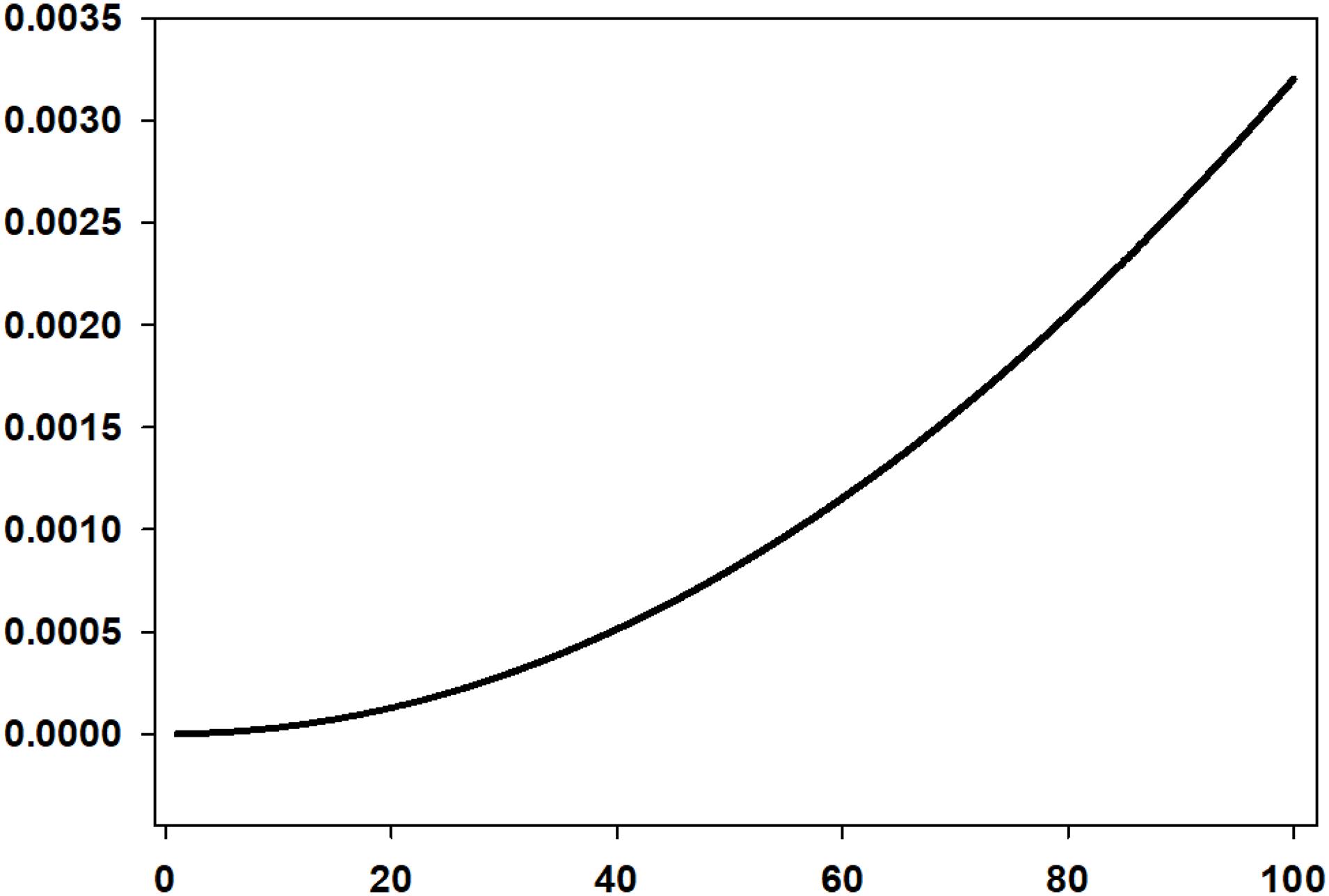
Figure 1. The rise rate of droplets of various sizes in the <100 μm range calculated using the Stokes relationship (This shows that droplets larger than about 50 μm do not reside in the water column for very long. The time for a 5 μm droplet to rise 1 m is 35 h, for a 16 μm droplet, 3.4 h, for a 50 μm droplet, 20 min and for a 100 μm droplet, 5 min).

Sea energy is a major factor in dispersion (Delvigne and Sweeney, 1988; Zeinstra-Helfrich et al., 2015a). There have been several representations of sea energy that have been used in oil spill modeling including wave height, wave steepness, wave period, wind speed, etc. (Parsa et al., 2016). Wave height has been used extensively in calculations. Studies have shown that steepness is an important parameter and the high energy of breaking waves is significant in producing dispersions (Delvigne and Sweeney, 1988; Zeinstra-Helfrich et al., 2015b). Studies have shown that wave height is equivalent to a plunging stream and therefore can be used as an indicator of sea energy (Zeinstra-Helfrich et al., 2015a; Parsa et al., 2016). Breaking waves are much more likely to disperse oil than non-breaking waves, in fact the increase may be up to 25% (Zeinstra-Helfrich et al., 2015b). Some researchers have noted poor dispersion in non-breaking waves (Zeinstra-Helfrich et al., 2015b). Turbulence is obviously a good indicator of sea energy; however, values of turbulence are not available to spill modelers except in wave tanks (Li and Garrett, 1998; Fingas, 2013a; Li et al., 2017; Pan et al., 2017; Wang and Zhang, 2019). It has been noted that there is low dispersion when winds are low, in fact no dispersion was seen in one sea trial where the winds were below 5 m/s (Zeinstra-Helfrich et al., 2015b).

The effect of oil layer thickness has been studied by researchers (Mackay et al., 1985; Zeinstra-Helfrich et al., 2015b, 2016). One group found that the dispersion rate or entrainment rate was directly proportional to the oil layer thickness. Despite this persuasive argument of including oil layer thickness, no current algorithm has included oil thickness in calculations, simply because it is not a parameter that is available to the spill responder. Zeinstra-Helfrich et al. (2016) conducted experiments with plunging jets and measured large droplets (in millimeter size range). These experiments showed that the amount of oil entrained (in large droplets) did depend on oil layer thickness. This entrainment was increased by the application of dispersants.

Several factors influence the chemical dispersion of oil into the sea. Oil temperature is one of these. Oil temperature is thought to be between the water temperature and the sea temperature in the daytime and at water temperature at night (Fingas, 2011). Temperature will be included in this model as the viscosity which varies with temperature.

The distribution of the oil through the water column has been measured by some researchers (Parsa et al., 2016). This group found that the mid-depth concentrations in their flume were 44–77% of the surface concentrations at the surface and that concentrations near the flume bed were 12–33% of the mid-depth concentrations. A simplification has appeared in other literature that the concentration is equally distributed in the water column to 1 1/2 times the wave height (Delvigne and Sweeney, 1988). This relationship will be used in this algorithm.

Algorithm Development

The present algorithm was constructed utilizing five basic processes. Initial dispersion was input using a modified Delvigne equation, then the droplet dispersion was distributed over the mixing depth as predicted by the wave height. The droplets rise to the surface according to Stokes’ law. The droplets in the water column are subject to coalescence as governed by the Smoluchowski equation. Some oil is “lost” in the process as a wide spectrum of droplet sizes are created. Very small droplets will rise only very slowly and may not be subject to re-dispersion. Oil on the surface, from the rising oil and that undispersed, is presumed re-dispersed. Figure 2 shows the process and end results of the modeling process.

FIGURE 2

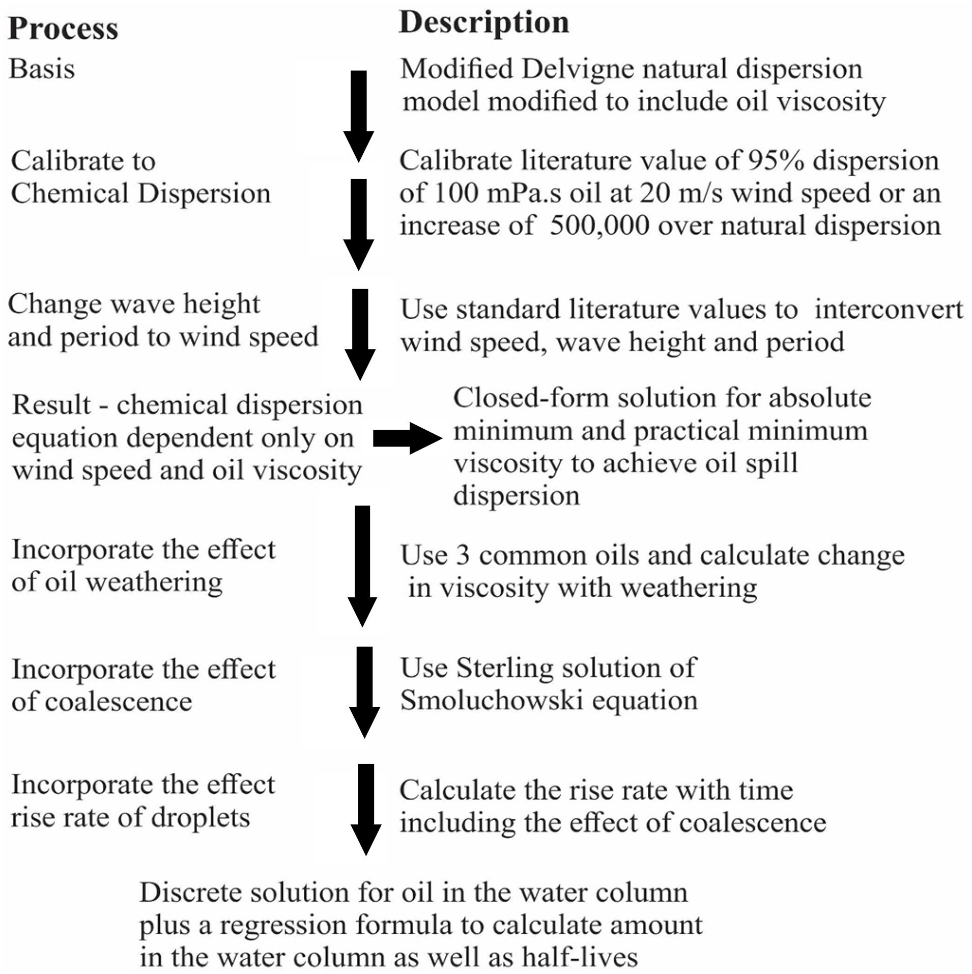
Figure 2. Overall summary of the modeling process in this study.

The starting point is the work of Delvigne carried out originally for natural dispersion (Delvigne and Sweeney, 1988; Delvigne, 1994; Fingas, 2013a; Johansen et al., 2015). The Delvigne work was based on extensive experimental work in large and medium-sized flumes. It is important in that it incorporates several important factors such as wind speed, wave height and wave period. The Delvigne model, as noted, was constructed using empirical data carried out over years and fortunately with modern techniques such as in situ laser particle size measurement and gas chromatography for oil content. Further, it is the only injection model which includes inputs of wind speed, wave height and period, as well as oil droplet size and oil type. This Delvigne work will improve the accuracy of current modeling of dispersed oil and increase its correspondence to reality.

Fingas (2013a) worked on this relationship and found that the constants were consistent with units of viscosity (mPa.s). Therefore, units of viscosity were used in further development:

$$F_{(d)}=\frac{6.3\times {10}^{-4}}{{\mathrm{\mu }}^{1.5}}{\left(34.4\times H_{rms}^2\right)}^{0.57}\left[\frac{0.032\left(U-5\right)}{T_w}\right](1)$$

where F_(d) is the fraction of entrained mass rate of droplet sizes in the interval from 10 to 30 μm given in fraction/hour. It should be noted that the time unit of 1 h will be used as the time step throughout this paper for consistency, μ is the viscosity of the oil in cP or mPa.s, H_rms is the r.m.s. value of the wave height (m), U is the wind speed in m/s, and T_w is the wave period in s.

The equation must be adjusted to oil dispersion using chemical dispersants, so setting the optimal conditions for oil dispersion using chemical dispersants at the 20 m/s wind, 8 m wave height, wave period of 11 s and oil viscosity of 100 mPa.s so that the dispersion at these conditions becomes 95% per hour, the constant in the equation becomes 284 (Fingas et al., 2003). This represents an increase of about 500,000 in the amount entrained by chemical dispersion over natural dispersion. The equation becomes:

$$F_{(d)}=\frac{284}{{\mathrm{\mu }}^{1.5}}{\left(34.4\times H_{rms}^2\right)}^{0.57}\left[\frac{0.032\left(U-5\right)}{T_w}\right](2)$$

where F_(d) is the fraction of entrained mass rate of droplet sizes in the interval from 10 to 30 μm given in hour, μ is the viscosity of the oil in mPa.s or cP, H_rms is the r.m.s. value of the wave height (m), U is the wind speed in m/s, and T_w is the wave period in s.

This equation inputs wind speed, wave height and wave period. As there is a relationship among these components in a fully arisen sea (equilibrium between wind and wave conditions), the equation can be simplified (Pierson and Moskowitz, 1964; Wikipedia, 2019). To achieve a fully arisen sea, the conditions in Table 1 are applied.

TABLE 1

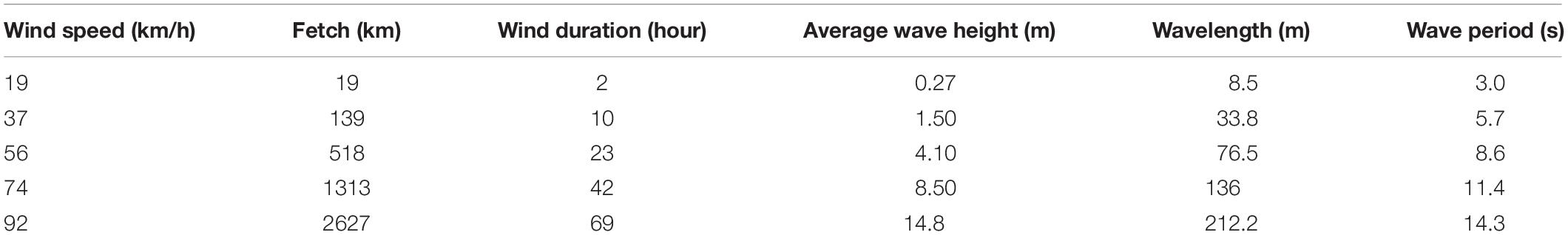
Table 1. Conditions to achieve a fully arisen sea (Wikipedia, 2019).

These conditions can then be used to develop relationships among wind speed, wave height and wave period be using regression and choosing a simple and appropriate algorithm. This is applicable to a fully arisen sea of the specified duration. The following relationships are obtained:

$$H_{rms}=0.0045U^2(3)$$

where H_rms is the r.m.s. value of the wave height (m), simply H from this point on, and U is the wind speed in m/s, the wave period T_w can be similarly related to wind as:

$$T_w=0.55U(4)$$

where U is the wind speed in m/s, and T_w is the wave period in second.

Substituting these wind equivalents in Eq. (2) one derives the dispersion equation in wind speed and oil viscosity only. Further the equation was multiplied by 100 to yield the output in percentage.

$$D_{isp\%}=449U^{2.28}\left(0.058-\frac{0.29}{U}\right)\frac{1}{{\mathrm{\mu }}^{1.5}}(5)$$

where D_isp% is the percent dispersed per hour, U is the wind speed in m/s, and μ is the viscosity of the oil in mPa.s or cP.

One of the factors that becomes important in the above relationship is that of oil viscosity. Oil viscosity increases with weathering. This typically varies with oil type (Guyomarch et al., 2012). In order to provide an estimate of the change in viscosity of oils, weathering data on several oils (Alaska North Slope, Louisiana, and Alberta Sweet Mixed) were combined and were correlated with time (Fingas, 2013). This is detailed further in the Supplementary Data. The weathering analysis yielded the following simplified relationship (R² = 0.85):

$$\mathrm{\mu }=3.8+0.35{\mathrm{\mu }}_{start}{t}_{hrs}(6)$$

where μ is the adjusted or viscosity of the weathered oil, μ_start is the starting oil viscosity, and t_hrs is the time in hours that the oil has weathered. At 0 h, μ = μ_start.

This relationship can then be used to correct oil viscosity for weathering before the dispersion process starts or re-starts in the case of re-dispersion. The longer the oil sits on the water before the dispersion process starts, the more viscous it becomes.

Viscosity changes with the oil temperature. Viscosity decreases with oil temperature increase. For example, one Alaska North Slope oil showed a viscosity of 13 mPa.s at 15°C and 17.8 mPa.s at 0°C. Another example is that of an Alberta crude oil which showed a viscosity of 8 mPa.s at 15°C and 26 mPa.s at 0°C. Adjustment to the actual oil viscosity at the oil temperature will account for temperature effects in the model.

The depth that droplets are injected into the water becomes an important factor (Parsa et al., 2016). Delvigne (1994) experimentally measured droplet injection and found that it was 1 1/2 times the wave height. This 1 1/2 factor will then be used to predict the depth to which droplets are injected with wave height.

The coalescence occurring in the water column is described by Smoluchowski (Hunter, 2001; Chavanis, 2019; Singh et al., 2020):

$$\frac{dn}{dt}=4\mathrm{\pi }{D}_{i}r{n}^2(7)$$

where dn/dt is the rate of diffusion-controlled coalescence, D_i is the diffusion coefficient cm²/s, r is the collision radius (distance between centers when coalescence begins), and n is the number of particles per cm³. The dn/dt can be viewed as the change in droplet distribution with coalescence.

Combining this equation with diffusion equations yields an expression for particle coalescence rate and thus for dispersion stability (Hunter, 2001):

$$\frac{d\overline{V}}{dt}=\frac{4}{3}\frac{VkT}{\mathrm{\mu }}{e}^{-E/kT}=A{e}^{-E/kT}(8)$$

where $d\overline{V}/dt$ is the rate of the coalescence of droplets or the stability of the dispersion, V is the volume of the dispersed phase (e.g., concentration), k is the Boltzmann constant, T is the absolute temperature, E is the energy barrier to coalescence, μ is the viscosity of the liquid continuous phase, and A is the collision factor as defined by the left portion of the equation. The Smoluchowski equation is used to describe the change in particle size distribution over a given volume and relates this distribution to energy.

This is the most important equation in describing the stability of oil-in-water emulsions as it shows that the volume and viscosity of the continuous phase (e.g., water), are limiting parameters in describing stability or increased coalescence (Hunter, 2001). In other words, oil spill dispersions in water will always have low stability because the water viscosity is low.

Sterling et al. (2004) performed extensive experiments in different laboratory systems and test tanks and developed a practical solution to Eq. (8). This work describes the change in particle size distribution with coalescence over time, given the same concentration in the measurement vessel. Filling in the variables for the CGS system of units and using the values from Sterling et al. (2004) for a system such as the one in this paper:

$$OD{S}_{new}=OD{S}_{old}+0.686OD{S}_{old}^{0.715}(9)$$

where ODS_new is the new oil droplet size in μm, for 1 h and for turbulence conditions as in the laboratory experiment, and ODS_old is the previous oil droplet size in μm.

The rise of the droplets through the water column to the surface is limiting and is governed by the Stokes rise time (Hunter, 2001). This is classically given by:

$$s=\frac{2\mathrm{\Delta }\mathrm{\rho }g{\mathrm{\alpha }}^2}{9\mathrm{\mu }}(10)$$

where s is the Stokes rise rate in m/s, Δρ is the density difference between the disperse and droplet phases, g is the gravitational constant in m/s², a is the droplet radius in m, and η is the viscosity of the continuous phase or the water.

Solving Eq. (10) for cgs units and typical oil densities:

$$s=3.2E^{-07}OD{S}^2(11)$$

where s is the Stokes rise rate in m/s, and ODS is the droplet diameter value of the droplet size in μm.

The starting droplet size chosen for this study is 16 μm as this is the typical Volume Mean Diameter size for an oil dispersion using chemical dispersants (Fingas and Ka’aihue, 2004; Fingas, 2011; Lehr et al., 2014). Other droplet sizes could be modeled using the inputs to Eq. (5).

The effect of the droplet size and the increase in droplet size as calculated using Eq. (9) is summarized in Table 2.

TABLE 2

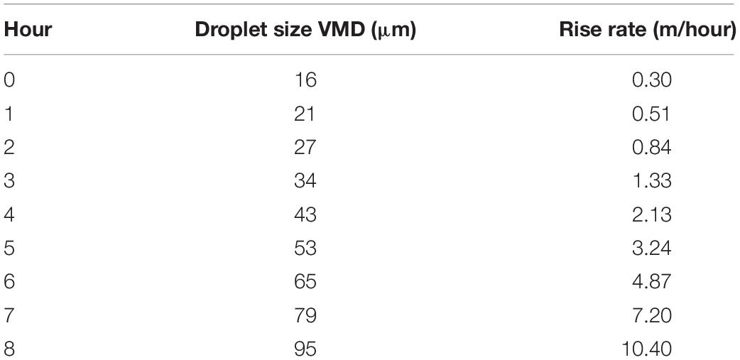
Table 2. Droplet size and rise rate.

The results of Table 2 can be reformulated using regression to yield a continuous rising rate dependent on time (R² = 0.99). This takes in account the increasing rise rate with time due to coalescence with the starting droplet size of 16 μm.

$$s=0.096+0.014t^{2.5}(12)$$

where s is the Stokes rise rate in m/sec, and t is the time in hours.

An important piece of information is the loss of oil and dispersed oil during the dispersion process (Fingas, 2010; Li et al., 2010). An important loss is the formation of very small oil droplets which rise only slowly and when resurfaced appear some distance away from the main slick. This present algorithm, as do most models, look only at the VMD or volume mean diameter, which is the mean of the cubic volume of droplets. This represents the diameter of the particle of the average volume of the mixture. The VMD lies close to the largest diameter of droplets which are in the mixture. Typically, there are many smaller droplets and often droplets that are one or two orders of magnitude smaller than that of the VMD sizes. These droplets will rise to the surface in hours and not minutes. Several estimates of this loss average range from 2 to 10% (Fingas, 2010; Li et al., 2010). These are the values which will be used in this study. A summary of the typical and extent of inputs appears in Table 3.

TABLE 3

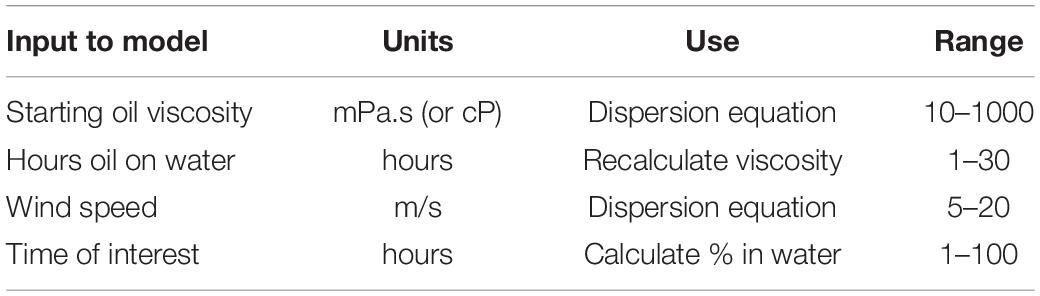
Table 3. Inputs to the algorithm.

Closed Form Solutions for Initial Oil Dispersion

It is possible to provide closed form solutions to the dispersion problem by substituting into Eq. (5). This covers the equation inputs up to Eq. (5) and therefore does not consider rise time etc. These will be considered in the section “Discrete Solutions” below. First, using 5% as the least dispersion that would be considered or a viscosity cut-off, set the equation to (Fingas, 2011):

$${\mathrm{\mu }}_{\max }^5=5=449U^{2.28}\left(0.058-\frac{0.29}{U}\right)\frac{1}{{\mathrm{\mu }}^{1.5}}(13)$$

where ${\mathrm{\mu }}_{\max }^5$ is the lowest or minimum dispersion possible with the wind and oil viscosity, U is the wind in m/s, and μ is the oil viscosity in mPa.s.

Solving Eq. (13) for the maximum viscosity, this becomes:

$${\mathrm{\mu }}_{\max }^5={\left[89.8\times U^{2.85}\left(0.058-\frac{0.29}{U}\right)\right]}^{0.67}(14)$$

where ${\mathrm{\mu }}_{\max }^5$ is the maximum viscosity (in mPa.s) to yield any dispersion at the given wind, and U is the wind in m/s.

To render a practical solution to this, a set of numbers calculated from Eq. (14) were regressed using TableCurve 2D. This yielded Eq. (15) (R² = 0.999):

$${\mathrm{\mu }}_{\max }^5=15.3+10.3U^2(15)$$

where ${\mathrm{\mu }}_{\max }^5$ is the maximum viscosity (in mPa.s) to yield dispersion at the given wind, and U is the wind in m/s.

The 5% is the value that is considered a minimum cut-off value for oil dispersion using chemical dispersants (Fingas, 2011). Considering the minimum useful oil dispersion using chemical dispersants, one can set a value of 30% (Fingas, 2011). This is a practical value below which it is questionable whether or not one is achieving a benefit. Thus, the dispersion equation becomes:

$${\mathrm{\mu }}_{\max }^{30}=30=449U^{2,28}\left(0.058-\frac{0.29}{H}\right)\frac{1}{{\mathrm{\mu }}^{1.5}}(16)$$

where ${\mathrm{\mu }}_{\max }^{30}$is the maximum viscosity (in mPa.s) to yield a practical dispersion at a given wind, and U is the wind in m/s and μ is the oil viscosity in mPa.s.

Solving Eq. (16), this becomes:

$${\mathrm{\mu }}_{max}^{30}=15H^{2.28}{\left\{0.058-\frac{0.29}{H}\right\}}^{0.67}(17)$$

where ${\mathrm{\mu }}_{\max }^{30}$ is the optimal maximum viscosity (in mPa.s) to yield 30% dispersion at the wave height, and H is the r.m.s wave height in m.

While exact solutions are desired, a more simplified solution can be created to provide a quick and simple solution. To render a practical solution of the maximum and maximum practical viscosity, a plot of values calculated using Eq. (17) were regressed using TableCurve 2D. This yields the equation (R² = 0.999):

$${\mathrm{\mu }}_{\max }^{30}=10.4+3.1U^2(18)$$

The results of these solutions are illustrated in Figure 3.

FIGURE 3

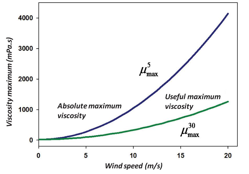
Figure 3. Plot of the absolute maximum viscosity and the useful maximum viscosity with wind speed.

Similar results can also be achieved for dispersion calculated with wave height. Calculating the weight height for Eq. (14) using the equivalency of Eq. (4), a table was generated and using regression in TableCurve 2D, the following simplest relationship is achieved (R² = 0.999):

$${\mathrm{\mu }}_{\max }^{30}=69.4+2285H(19)$$

where ${\mathrm{\mu }}_{\max }^{30}$ is the maximum viscosity (in mPa.s) to yield 5% dispersion at the wave height, and H is the r.m.s wave height in m.

Performing the same calculation for 30% as the least useful dispersion, one arrives at (R² = 0.999):

$${\mathrm{\mu }}_{\max }^{30}=20.9+689H(20)$$

where ${\mathrm{\mu }}_{\max }^{30}$ is the optimal maximum viscosity (in mPa.s) to yield 30% dispersion at the wave height, and H is the r.m.s wave height in m. These wave height and viscosity calculations are illustrated in Figure 4.

FIGURE 4

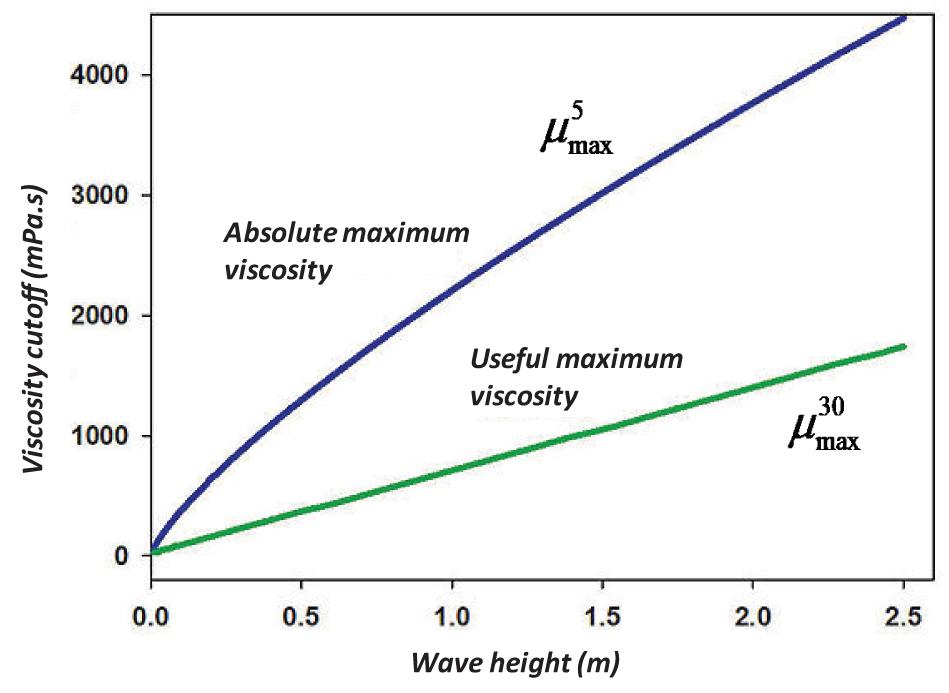
Figure 4. Plot of the practical maximum viscosity and the useful maximum viscosity with wave height.

Discrete Solutions

The data are available to be able to calculate dispersion values at each hourly step. The only inputs needed are the time in hours after application of dispersants, the wind speed (m/s) and the oil viscosity (mPa.s). The calculations are different for the first-time step (0 or zero) than for the remaining time steps.

$${\%}_W^0={\%}_W^{prev}-{\%}_{loss}(21)$$

where ${\%}_W^0$ is the percentage in the water at time 0; ${\%}_W^{prev}$ is the percentage in the water as predicted by Eq. (5) and %_loss are the small droplets that would not rise in the time of concern here (generally less than 1 day). Examination of a droplet count from a typical dispersion shows that about 5% of the droplets are less than 1 μm (Fingas, 2010). These droplets certainly would rise slowly, more than 150 h from 2 m. Five percent loss will be used in the example calculation here.

Thereafter, the calculation becomes:

$${\%}_W^t={\%}_W^{prev}-{\%}_{Rise}+{\%}_{re-disp}+{\%}_{loss}(22)$$

where ${\%}_W^t$ is the percentage in the water at time t; ${\%}_W^{prev}$is the previous percentage in the water; %_Rise is the percent rising; %_re−disp is the amount re-dispersed; and %_loss is the percent loss as small droplets (here taken as 5%, as an example).

To calculate the portions of Eq. (22) one needs:

$$D_{Disp}=1.5H=0.0067U^{0.5}(23)$$

where D_Disp is the depth of dispersion (m); H is wave height (m) and U is the wind speed (m/s).

$$t_{rise}=D_{Disp}/s(24)$$

where t_rise is the rise time (hours); D_Disp is the depth of dispersion (m) and s is the rise rate (m/s) from Eq. (12).

$$F_{rise}=t_{rise}/t_{int}(25)$$

where F_rise is the fraction rising; t_rise is the rise time (hours); and t_int is the time of interest

$${\%}_{rise}=100F_{rise}(26)$$

where %_Riseis the percent rising, and F_rise is the fraction rising.

Redispersion is calculated using the equations above and new viscosity calculated using Eq. (7). Fraction of oil to be re-dispersed equals the amount rising in Eq. (25).

$${\%}_{rise-disp}=F_{disp}+{\%}_{disp}(27)$$

where %_re−disp is the percent re-dispersed; F_disp is the fraction to be re-dispersed; %_disp is the amount dispersed dependent on input conditions [Eq. (5)].

This will result in values in the water column at each point of time. The amount on the surface (%_surf) will be:

$${\%}_{surf}=100-{\%}_W^t(28)$$

where %_surf is the percent of oil on the surface and ${\%}_W^t$ is the percent in the water column at that time.

Table 4 shows a summary example calculation. Detailed calculations and examples are given in the Supplementary Material.

TABLE 4

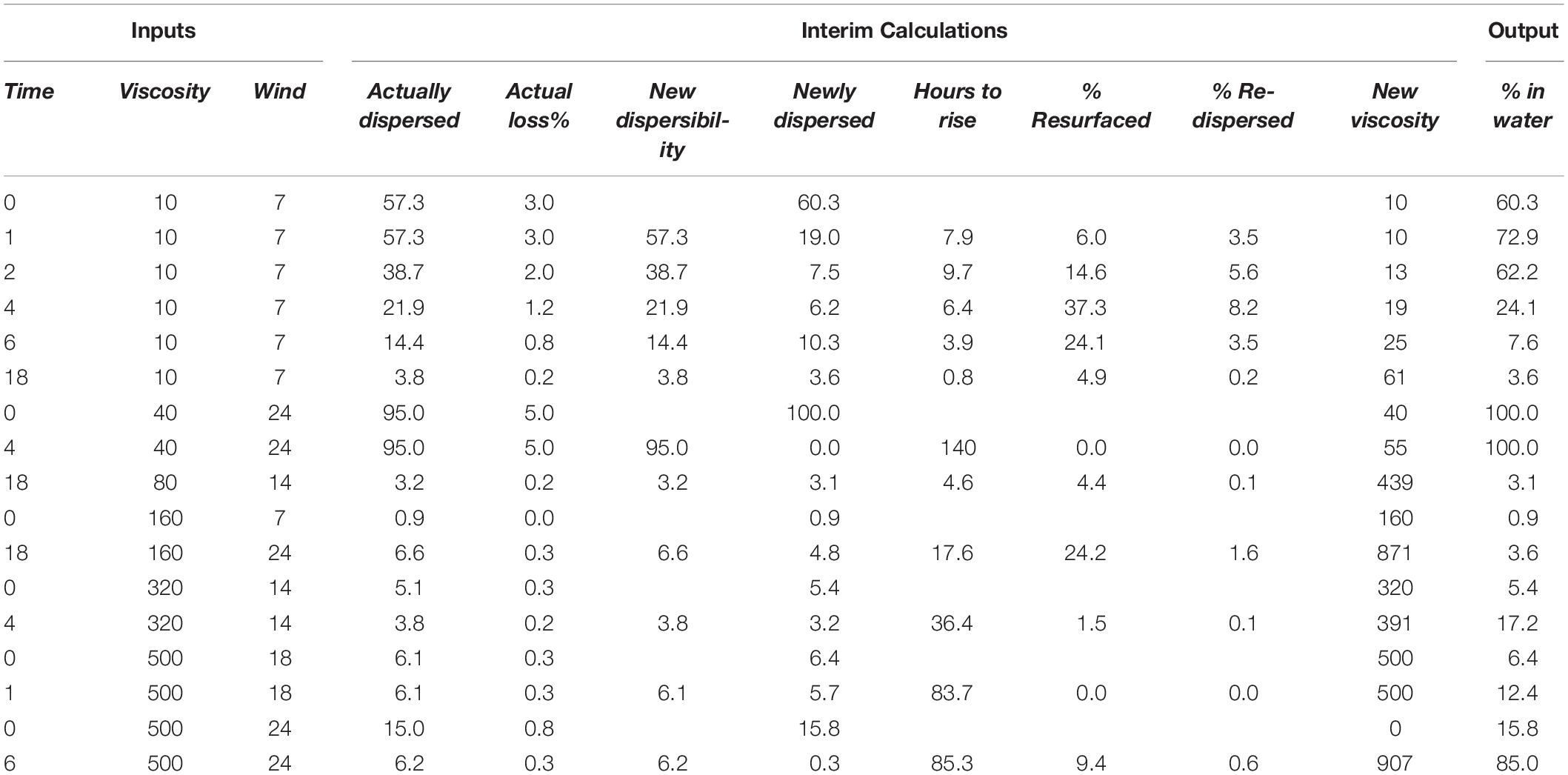
Table 4. Example of a discrete calculation spread sheet.

The entire results from the spreadsheet of sample calculations as described in detail in the Supplementary Material, were regressed using DataFit (Oakdale Engineering) to derive an optimal (highest correlation coefficient) continuous equation to predict the percent in water given time, viscosity and wind inputs (R² = 0.73):

$${\%}_W^t=22.6-3.7\left(t\right)-0.13\left(\mathrm{\mu }\right)+3.87\left(U\right)(29)$$

where ${\%}_W^t$ is the percent in the water column at the chosen time (hours), t is the time (hours), μ is the oil viscosity (mPa.s) and U is wind speed (m/s). This simplified equation represents a rapid calculation method to estimate percentage in the water column.

The results of Eq. (29) require correction to maintain effectiveness values between 0 and 100%. Eq. (29) includes the loss of 5% to account for the loss of small droplets.

The maximum dispersed amount data were extracted from the original discrete calculation spreadsheet. These maximum values were then correlated with the oil viscosity and the wind speed at which they occurred using TableCurve 3D (SigmaPlot, San Jose, CA, United States) (R² = 0.76). The predictor equation is given below:

$${\%}_{Max}=202-18.2\ln \left(\mathrm{\mu }\right)-746/\left(U\right)(30)$$

where %_Max is the maximum percent in the water, μ is the oil viscosity (mPa.s) and U is wind speed (m/s).

The results of Eq. (30) require correction to maintain effectiveness values between 0 and 100%. Figure 5 shows the maximum amount of oil in the water column given oil viscosity and wind speed.

FIGURE 5

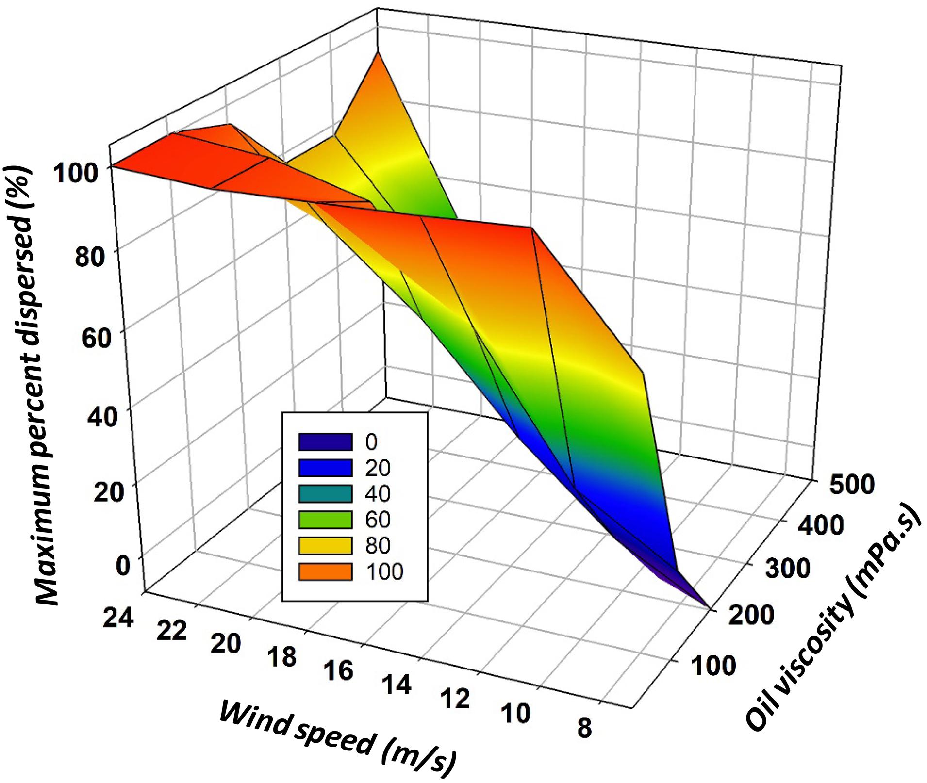
Figure 5. The maximum predicted amount in the water column given an oil viscosity and wind speed using Eq. (30).

This type of spreadsheet calculation also allows the calculation of the half-life. The half-life can be a criterion for the success of a dispersion (Fingas, 2010). The half-lives of the entire spreadsheet created for the above exercise, were calculated using the spreadsheet describe above as input. The half-life of any process can be described as:

$$T_{1/2}=\mathrm{\tau }\times \ln \left(2\right)(31)$$

Taking τ as the mean lifetime (in hours) as the time calculated from Eq. (29), the following expression can be derived:

$$T_{1/2}=-\left[72.6-0.32\left(\mathrm{\mu }\right)+3.87\left(U\right)\right](0.187)(32)$$

Results and Discussion

Algorithm Assessment

A model of oil dispersion using chemical dispersants was published in recent years by Johansen et al. (2015). The model was developed from a theoretical point of view and then fit to experimental data from a field experiment and some wave tank work. A simplified version of this was developed as well:

$$\frac{\partial Q_s}{\partial t}=\mathrm{\alpha }{C}_s(33)$$

where ∂Q_s/∂t is the rate of mass disappearance (kg/s), C_s is the starting mass in kg, and

$$\mathrm{\alpha }=\left(pWCC\right)/T_m(34)$$

where in turn, p is the volume fraction of oil contained in oil droplets smaller than the limiting diameter D^∗, here taken as 0.00054 tenths of m or 54 μm, WCC is the white cap coverage, which as suggested by Johansen et al. (2015) is:

$$WCC(\%)=3.18\times {10}^{-3}{(U-3.7)}^3\mathit{\hspace{1em}}\text{(for wind speeds}\mathit{\hspace{1em}}\text{between 3.7 and 11.25 m/s)}(35)$$

$$WCC(\%)=4.82\times {10}^{-4}{(U+1.98)}^3\mathit{\hspace{1em}}\text{(for wind speeds}\mathit{\hspace{1em}}\text{between 9.25 and 23.1 m/s)}(36)$$

T_m is the wave period (in m), which can be given as Eq. (5) or 0.55 × wind. Eq. (33) can be solved by converting it into percentage by multiplying C_s by 100. Similarly dividing by 3600 will convert the equation into% per hour to be consistent with the values used in this paper. The following equations result:

$$C=0.636{\left(U-3.7\right)}^3/0.55U\mathit{\hspace{1em}}\text{(for wind speeds between}\text{3.7 and 11.25 m/s)}(37)$$

$$C=0.0964{\left(U+1.98\right)}^4/0.55U\mathit{\hspace{1em}}\text{(for wind speeds between}\text{9.25 and 23.1 m/s)}(38)$$

where C is the percent dispersed per hour, and U is the wind speed in m/s.

This model is compared with the results of the current model as shown in Figure 6.

FIGURE 6

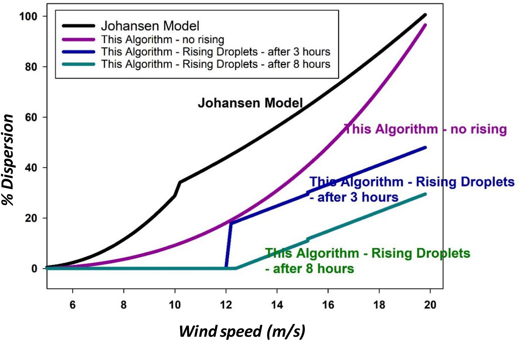
Figure 6. A comparison of the Johansen model, this paper’s algorithm without rising effects, and two instances of algorithms from this paper with the effects of droplet rising.

The present model was solved for this figure using Eq. (5) for the dispersion which does not consider droplet rising. For the calculations that used the effect of droplet rising, Eq. (29) was used. The parameters for this paper’s models were set as oil with 100 mPa.s viscosity, and those with the rising effect were taken at 3 and 8 h, and input loss rate of 5.

Figure 6 shows that the Johansen et al. (2015) model resulted in very similar outputs to the algorithm in this study as calculated by Eq. (5), but without the effects of droplet rising. The addition of droplet rising considerations reduced the amount dispersed.

Overall Results

An algorithm for predicting the oil dispersion using chemical dispersants was developed using an empirical natural dispersion model by Delvigne as a beginning approach to a five-step solution. This natural dispersion model was first modified by substituting oil viscosity for constants in the equation. Second, the model was calibrated to a chemical dispersion situation by adjusting the equation to yield 95% initial dispersant effectiveness for a 100 mPa.s oil. This adjustment involves a factor of about 500,000 adjustment to the equation’s constant. The essential feature of the developed algorithm is that it considers the injection of droplets, the subsequent rising and coalescence of these droplets to the surface. Since dispersion involves a wide spectrum of droplet sizes, it is calculated here that the very small droplets (less than about 1 μm) do not rise in sufficient abundance to reform slicks. Droplets are injected to a depth of one and a half times the significant wave height into the water column. The droplets that are rising are subject to coalescence as predicted by the Smoluchowski equation. The coalescence effect is profound and results in almost 50%increase in droplet size per hour and nearly an exponential decrease in their rise time.

The present algorithm includes the properties of the oil (viscosity), droplet size, as well as wave conditions and wind conditions, all predicted by the wind speed.

Conclusion

The primary findings realized by this developed algorithm include the following:

i The dispersion is most dependent on the wind speed. A minimum wind speed can be calculated for each viscosity. Even at low viscosities of around 10 mPa.s, the minimum wind speed to achieve dispersion is around 7 m/s.

ii The second most dependent factor for dispersion is the viscosity of the oil, a proxy for the composition. Higher viscosities require higher winds to achieve even a little dispersion. Furthermore, weathering of the oil increases the viscosity leading to a time cut-off when dispersion is no longer-possible.

iii Inputs to calculation are reduced to wind speed and oil starting viscosity. Time of interest can be used to examine the percent of oil in the water column. This work also noted that some of the oil, estimated here as 5% or the percent of the droplets below 1 μm, would not rise in time to influence the calculation and thus could be considered to be ‘lost.’ The “5%” is 5% of the oil being dispersed or re-dispersed and not the whole oil amount.

iv The coalescence in droplets was calculated according to other experiments in the literature. The result is that as time progresses the droplets increase in size and rise more rapidly. The progression is approximately exponential.

v Closed form solutions are provided to calculate the maximum practical viscosity to achieve any type of dispersion for a given wind speed. Discrete calculation procedures are given to calculate concentration in the water column at given times, oil viscosity and wind speed.

Comparison of the present algorithm with another model showed that the base algorithm yielded similar results, without the consideration of the rise and coalescence of the droplets in the water column. The following conclusions could be drawn from this algorithm:

i Wind speed and oil viscosity were dominant factors in controlling dispersion process. While higher viscosities require higher winds to achieve dispersion, the minimum wind speed to achieve dispersion was around 7 m/s.

ii An exponential growth in coalescence size was observed. As the time passed, the droplets increased in size and rise more rapidly.

iii Closed form solutions along with discrete calculation procedures were developed to calculate the concentration in the water column with no rising considered.

Data Availability Statement

The original contributions presented in the study are included in the article/Supplementary Material, further inquiries can be directed to the corresponding author.

Author Contributions

MF: conceptualization, research plan, supervision, experiments, and data analysis. MF, KY, and MB: investigation, writing, review, and editing. MF and KY: writing original draft preparation. All authors discussed the results, contributed to the final manuscript, read and agreed to the published version of the manuscript.

Funding

This work was entirely self-funded by the authors.

Conflict of Interest

The authors declare that the research was conducted in the absence of any commercial or financial relationships that could be construed as a potential conflict of interest.

Supplementary Material

The Supplementary Material for this article can be found online at: https://www.frontiersin.org/articles/10.3389/fmars.2020.600614/full#supplementary-material

References

Chavanis, P.-H. (2019). The generalized stochastic Smoluchowski equation. Entropy 21:1006. doi: 10.3390/e21101006

CrossRef Full Text | Google Scholar

Delvigne, G. A. L. (1994). Natural and chemical dispersion of oil. J. Adv. Mar. Technol. Conf. 11, 23–40.

Google Scholar

Delvigne, G. A. L., and Sweeney, C. E. (1988). Natural dispersion of oil. Oil Chem. Pollut. 4, 281–310. doi: 10.1016/s0269-8579(88)80003-0

CrossRef Full Text | Google Scholar

ESTS (2018). Oil Properties Data Base. Available online at: http://www.etc-cte.ec.gc.ca/databases/oilproperties/ (accessed November 12, 2018).

Google Scholar

Fingas, M. (2010). “Models of Oil Spill Dispersion Stability,” in Proceedings of the Thirty-third Arctic and Marine Oil Spill Program Technical Seminar, Environment Canada, Ottawa, ON, 555–586.

Google Scholar

Fingas, M. (2011). “Oil Spill Dispersants: A Technical Summary,” in Oil Spill Science and Technology, ed. M. Fingas (New York, NY: Gulf Publishing Company), 435–582. doi: 10.1016/b978-1-85617-943-0.10015-2

CrossRef Full Text | Google Scholar

Fingas, M. (2013a). “A Review of Natural Dispersion Models,” in Proceedings of the Thirty-Sixth Arctic and Marine Oil Spill Program Technical Seminar, Environment Canada, Ottawa, ON, 207–233.

Google Scholar

Fingas, M. (2013). Modeling oil and petroleum evaporation. J. Petrol. Sci. Res. 2:104.

Google Scholar

Fingas, M. F., and Ka’aihue, L. (2004). “Dispersant Field Testing - A Review of Procedures and Considerations,” in Proceedings of the Twenty-Seventh Arctic and Marine Oil Spill Program Technical Seminar, Environment Canada, Ottawa, ON, 1017–1046.

Google Scholar

Fingas, M. F., Wang, Z., Fieldhouse, B., and Smith, P. (2003). “The Correlation of Chemical Characteristics of an Oil to Dispersant Effectiveness,” in Proceedings of the Twenty-Sixth Arctic and Marine Oil Spill Program Technical Seminar, Environment Canada, Ottawa, ON, 679–730.

Google Scholar

Guyomarch, J., Le Floch, S., and Jezequel, R. (2012). “Oil Weathering, Impact Assessment and Response Options Studies at the Pilot Scale: Improved Methodology and Design of a New Dedicated Flume Test,” in Proceedings of the 35th AMOP Technical Seminar on Environmental Contamination and Response, Brest, 1001–1017.

Google Scholar

Hunter, R. J. (2001). Foundations of Colloid Science, 2nd Edn. Oxford: Oxford University Press, 806.

Google Scholar

Johansen, T., Reed, M., and Bodsberg, M. R. (2015). Natural dispersion revisited. Mar. Pollut. Bull. 93, 20–26. doi: 10.1016/j.marpolbul.2015.02.026

PubMed Abstract | CrossRef Full Text | Google Scholar

King, T., Robinson, B., Ryan, S., Lee, K., Boufadel, M., and Clyburne, J. (2018). Estimating the usefulness of chemical dispersant to treat surface spills of oil sands products. J. Mar. Sci. Eng. 6:128. doi: 10.3390/jmse6040128

CrossRef Full Text | Google Scholar

Lehr, W., Simecek-Beatty, D., Aliseda, A., and Boufadel, M. (2014). “Review of Recent Studies on Dispersed Oil Droplet Distribution,” in Proceedings of the 37th AMOP Technical Seminar on Environmental Contamination and Response, Ottawa, ON, 1–8.

Google Scholar

Li, M., and Garrett, C. (1998). The relationship between oil droplet size and upper ocean turbulence. Mar. Pollut. Bull. 36, 961–970. doi: 10.1016/s0025-326x(98)00096-4

CrossRef Full Text | Google Scholar

Li, Z., Lee, K., King, T., Boufadel, M. C., and Venosa, A. D. (2008). “Oil Droplet Size Distribution as a Function of Energy Dissipation Rate in An Experimental Wave Tank,” in Proceedings of the International Oil Spill Conference - IOSC, New Orleans, 621–626. doi: 10.7901/2169-3358-2008-1-621

CrossRef Full Text | Google Scholar

Li, Z., Lee, K., King, T., Boufadel, M. C., and Venosa, A. D. (2009). Evaluating chemical dispersant efficacy in an experimental wave tank: 2-significant factors determining in-situ oil droplet size distribution. Environ. Eng. Sci. 26, 1407–1418. doi: 10.1089/ees.2008.0408

CrossRef Full Text | Google Scholar

Li, Z., Lee, K., King, T., Boufadel, M. C., and Venosa, A. D. (2010). Effects of temperature and wave conditions on chemical dispersion efficacy of heavy fuel oil in an experimental flow-through wave tank. Mar. Pollut. Bull. 60, 1550–1559. doi: 10.1016/j.marpolbul.2010.04.012

PubMed Abstract | CrossRef Full Text | Google Scholar

Li, Z., Spaulding, M. L., and French-McCay, D. (2017). An algorithm for modeling entrainment and naturally and chemically dispersed oil droplet size distribution under surface breaking wave conditions. Mar. Pollut. Bull. 119, 145–152. doi: 10.1016/j.marpolbul.2017.03.048

PubMed Abstract | CrossRef Full Text | Google Scholar

Loh, A., Shankar, R., Ha, S. Y., An, J. G., and Yim, U. H. (2020). Stability of mechanically and chemically dispersed oil: effect of particle types on oil dispersion. Sci. Total Environ. 716:135343. doi: 10.1016/j.scitotenv.2019.135343

PubMed Abstract | CrossRef Full Text | Google Scholar

Mackay, D. (1985). “Chemical Dispersion: A Mechanism and a Model,” in Proceedings of the Eighth Arctic Marine Oilspill Program Technical Seminar, Environment Canada, Ottawa, ON, 260–268.

Google Scholar

Mackay, D., Chau, A., Hossain, K., and Bobra, M. (1985). “Measurement and Prediction of the Effectiveness of Oil Spill Chemical Dispersants,” in Oil Spill Chemical Dispersants: Research, Experience and Recommendations: STP 840, American Society for Testing and Materials, ed. T. E. Allen (Philadelphia, PA: ASTM International), 38–54. doi: 10.1520/stp30227s

PubMed Abstract | CrossRef Full Text | Google Scholar

Mukherjee, B., Wrenn, B. A., and Ramachandran, P. (2012). Relationship between size of oil droplet generated during chemical dispersion of crude oil and energy dissipation rate: dimensionless, scaling, and experimental analysis. Chem. Eng. Sci. 68, 432–442. doi: 10.1016/j.ces.2011.10.001

CrossRef Full Text | Google Scholar

Nissanka, I. D., and Yapa, P. D. (2017). Oil slicks on water surface: Breakup, coalescence, and droplet formation under breaking waves. Mar. Pollut. Bull. 114, 480–493. doi: 10.1016/j.marpolbul.2016.10.006

PubMed Abstract | CrossRef Full Text | Google Scholar

Pan, Z., Zhao, L., Boufadel, M. C., King, T., Robinson, B., Conmy, R., et al. (2017). Impact of mixing time and energy on the dispersion effectiveness and droplets size of oil. Chemosphere 166, 246–254. doi: 10.1016/j.chemosphere.2016.09.052

PubMed Abstract | CrossRef Full Text | Google Scholar

Parsa, R., Kolahdoozan, M., and Moghaddam, M. R. A. (2016). Vertical oil dispersion profile under non-breaking regular waves. Environ. Fluid Mech. 16, 833–844. doi: 10.1007/s10652-016-9456-1

CrossRef Full Text | Google Scholar

Pierson, W. J. J., and Moskowitz, L. A. (1964). Proposed spectral form for fully developed wind seas based on the similarity theory of S. A. Kitaigorodskii. J. Geophys. Res. 69, 5181–5190. doi: 10.1029/jz069i024p05181

CrossRef Full Text | Google Scholar

Reed, M., Daling, P., Lewis, A., Ditlevsen, M. K., Brørs, B., Clark, J., et al. (2004). Modelling of dispersant application to oil spills in shallow coastal waters. Environ. Model. Softw. 19, 681–690. doi: 10.1016/j.envsoft.2003.08.014

CrossRef Full Text | Google Scholar

Rosen, M. J., and Kunjappu, J. T. (2012). Surfactants and Interfacial Phenomena, 4th Edn. New York, NY: Wiley Interscience. doi: 10.1002/9781118228920

CrossRef Full Text | Google Scholar

Singh, M., Matsoukas, T., and Walker, G. (2020). Mathematical analysis of finite volume preserving scheme for nonlinear Smoluchowski equation. Phys. Nonlinear Pheno. 402:132221. doi: 10.1016/j.physd.2019.132221

CrossRef Full Text | Google Scholar

Sterling, M. C., Bonner, J. S., Ernest, A. N. S., Page, C. A., and Autenreith, R. L. (2004). Chemical dispersant effectiveness testing: influence of droplet coalescence. Mar. Pollut. Bull. 48, 969–977. doi: 10.1016/j.marpolbul.2003.12.003

PubMed Abstract | CrossRef Full Text | Google Scholar

Wang, J. H., and Zhang, J. S. (2019). Specification of turbulent diffusion by random walk method for oil dispersion modeling. Appl. Mech. Mater. 21, 1161–1167. doi: 10.4028/www.scientific.net/amm.212-213.1161

CrossRef Full Text | Google Scholar

Wikipedia (2019). Wind Wave. (accessed November 15, 2018).

Google Scholar

Zeinstra-Helfrich, M., Koops, W., Dijkstra, K., and Murk, A. J. (2015a). Quantification of the effect of oil layer thickness on entrainment of surface oil. Mar. Pollut. Bull. 96, 401–409. doi: 10.1016/j.marpolbul.2015.04.015

PubMed Abstract | CrossRef Full Text | Google Scholar

Zeinstra-Helfrich, M., Koops, W., Dijkstra, K., and Murk, A. J. (2016). How oil properties and layer thickness determine the entrainment of spilled surface oil. Mar. Pollut. Bull. 110, 184–193. doi: 10.1016/j.marpolbul.2016.06.063

PubMed Abstract | CrossRef Full Text | Google Scholar

Zeinstra-Helfrich, M., Koops, W., Dijkstra, K., and Murk, A. J. (2017). Predicting the consequence of natural and chemical dispersion for oil slick size over time. J. Geophys. Res. Oceans 122, 7312–7324. doi: 10.1002/2017jc012789

CrossRef Full Text | Google Scholar

Zeinstra-Helfrich, M., Koops, W., and Murk, A. J. (2015b). The NET effect of dispersants - A critical review of testing and modelling of surface oil dispersion. Mar. Pollut. Bull. 100, 102–111. doi: 10.1016/j.marpolbul.2015.09.022

PubMed Abstract | CrossRef Full Text | Google Scholar