Extreme Levels of Ocean Acidification Restructure the Plankton Community and Biogeochemistry of a Temperate Coastal Ecosystem: A Mesocosm Study

Introduction

The world oceans currently absorb 2.5 ± 0.5 GtC y^–1 of the total 11.5 ± 0.9 GtC y⁻¹ anthropogenic CO₂ emissions [2009 – 2018, Friedlingstein et al. (2019)]. The uptake of CO₂ by the oceans reduces global warming, but CO₂ dissolution in seawater results in the formation of carbonic acid, whose dissociation decreases average seawater pH – a process generally termed ocean acidification (OA) (Caldeira and Wickett, 2003; Emerson and Hedges, 2008). Realistic emission scenarios project that the pH of ocean surface waters will further decline by at least 0.2 units to about 7.9 by the end of the century [IPCC scenario RCP4.5, Pörtner et al. (2014)]. The effects of this alteration in the carbonate systems of the oceans on the inherent marine organisms has already been targeted by a variety of different experiments and approaches (Gattuso and Hansson, 2011). Within these studies, the observed consequences for marine plankton communities are diverse, indicating that the increased CO₂/decreased pH might put some marine species at advantage (e.g., diatoms) and others at disadvantage (e.g., calcifiers such as gastropods, molluscs) (Orr et al., 2005; Kroeker et al., 2013; Wittmann and Pörtner, 2013). In addition, recent studies have shown that consequences of an elevated partial pressure of CO₂ (pCO₂) also vary strongly between different oceanic regions as well as between planktonic communities (Fabricius et al., 2011; Riebesell et al., 2013b; Paul et al., 2015; Gazeau et al., 2017; Taucher et al., 2017). What they have in common, however, is that although the studies cover plankton communities in e.g., the Baltic Sea, the north western Mediterranean, the eastern subtropical North Atlantic or the Artic, they all discovered OA effects in similar trophic positions. Riebesell et al. (2013b) and Paul et al. (2015) both discovered predominantly positive effects of an OA simulation on pico- and nanophytoplankton organisms, along with corresponding changes in chl a or particulate organic matter (POM). Taucher et al. (2017), additionally, observed a pronounced reorganization of the whole plankton community under elevated pCO₂, still suspected to be driven by phytoplankton, but contrary to the other studies also affecting micro- and mesozooplankton organisms (Algueró-Muñiz et al., 2019).

In contrast to open ocean environments, coastal regions already experience seasonal/temporal pH conditions as low as or even lower than the 7.9 projected for the RCP4.5 end of the century scenario (Feely et al., 2008; Fassbender et al., 2011; Hofmann et al., 2011; Mcneil et al., 2011). For example, Feely et al. (2008) found pH values of 7.75 and below at the coast line of western North America from central Canada to northern Mexico, and Fassbender et al. (2011) reported pH values as low as 7.6, with pCO₂ exceeding 1100 μatm, at the coast of California during upwelling events. These near shore pCO₂ values were nearly three times higher than those found off shore. Extreme pH events like the one monitored in the California upwelling region occur episodically in short- or medium-term intervals (days to weeks), and result in substantial changes in carbonate chemistry, including increasing pCO₂, dissolved inorganic carbon (DIC), and calcite/aragonite corrosiveness of the seawater. Coastal plankton communities may harbor species that are well adapted to cope with these extreme conditions, while others may be living on the verge of their physiological capacities. This issue is especially eminent when considering that the scales and frequency of such pH events could increase in the future due to intensification of coastal upwelling, concurrent with end-of-the-century climate change projections (Hofmann et al., 2011; Sydeman et al., 2014). Although a lot of studies have already targeted OA and its impacts on marine organisms, experiments suitable to assess the consequences of enhanced extreme pH events on coastal ecosystems and their plankton community structures are rare. When investigating community-level changes, the majority of studies focused on pCO₂ values within the IPCC RCP4.5 end of the century projections or such that were just slightly exceeding them [see Lischka et al. (2017) and Bach et al. (2016) or meta-analysis by Kroeker et al. (2010)]. When higher pCO₂ values were applied, experiments were often either conducted in laboratory setups [e.g., Berge et al. (2010), Nielsen et al. (2010) and Rossoll et al. (2013)], focused on lower trophic level dynamics in natural settings (Calbet et al., 2014; Thomson et al., 2016; Bach et al., 2017) or on specific ecosystem key taxa such as calcifiers or appendicularians [see Thomsen et al. (2010), Lischka et al. (2011) and Bouquet et al. (2018)]. Apart from that, even these large-scale experiments still stayed beneath the pCO₂ values presumed here for future coastal areas that could reach a drop in pH of 0.4 units under a RCP8.5 scenario (Pörtner et al., 2014), thus leaving unclear, how coastal plankton communities might cope with future extreme pH events. To approach this uncertainty we conducted a large-scale in-situ mesocosm experiment enclosing a natural coastal plankton community in Raunefjord, Norway, and tested the two hypotheses of (1) plankton community composition/structure will change under extreme pH values, and (2) extreme pH will accordingly influence the biogeochemistry in the enclosed ecosystem.

Materials and Methods

Study Site

Raunefjord is a 15 km long and 4 km wide fjordlike strait on the southwest coast of Norway close to the city of Bergen (Figure 1B), and is assigned to the North Sea ecoregion with microtidal and euryhaline conditions (Molvær et al., 2007). Due to the wind-induced Norwegian Coastal Current, water masses are subject to a fast exchange with high salinity Atlantic deep water. The surface layer in the fjord typically shows a salinity around 30 with a pycnocline of up to 34.5 at depths between 100 m (winter/autumn) and 50 m (summer) (Helle, 1978; Molvær et al., 2007). The mesocosms were deployed at 60°15′55′′N, 5°12′21′′E in the vicinity of the Espegrend Marine Research Field Station, north-west off the island of Nordre Egdholmen, where water depths ranged from 50 to 75 m.

FIGURE 1

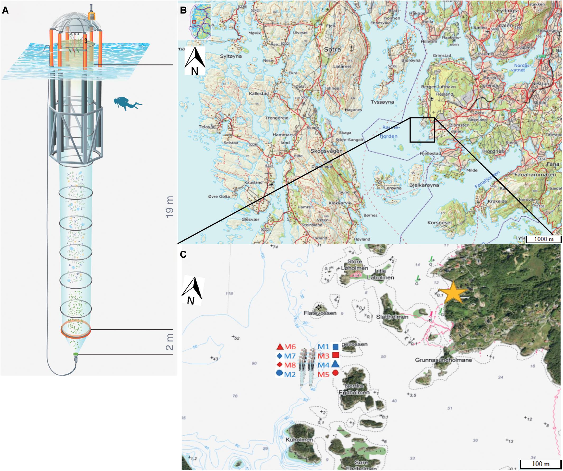
Figure 1. (A) Kiel Off-Shore Mesocosm for Ocean Simulations (KOSMOS), a pelagic mesocosm system. Blue corrugated area represents water surface. Diver for scale. Illustration of the KOSMOS unit by Rita Erven (GEOMAR), reprinted with permission from the AGU. (B) Location of Raunefjord between the island Sotra (left) and the city of Bergen (right). Black square indicates deployment area of the mesocosms. (C) Position, order and corresponding symbols of the mesocosms in their deployment area in front of the Espegrend Marine Research Field Station (marked by the yellow star), Bergen (not to scale). Red mesocosm numbers indicate high pCO₂ treatments, blue ones the control treatment. (B,C) Map modified after: The Norwegian Mapping Authority (Kartverket, accessed 7th July 2020, http://geo.ngu.no/kart/arealisNGU/). Figure assembled and designed with Adobe Illustrator CS4 (Adobe-Inc, 2008).

The “KOSMOS” Facility

The Kiel Off-Shore Mesocosms for Ocean Simulations (KOSMOS) are mobile, pelagic mesocosms (Riebesell et al., 2013a). Each mesocosm unit consists of a floating frame with a dome-shaped hood, the mesocosm bag, and a full diameter sediment trap sealing the bottom end of the bags (Figure 1A). The dimensions of the mesocosm enclosure in this study were 2 m in diameter and 21 m in length, resulting in an enclosed water volume of 56 m³ to 61 m³ (Table 1). The mesocosm bags are made of a flexible thermoplastic polyurethane foil, strongly reducing UV-light, but permitting similar light intensities and depth profiles of light in the photosynthetically active radiation (PAR) spectrum inside the mesocosms as in the surrounding water masses. The hoods on top of the floating frame reduce rainfall into the enclosures and are equipped with metal spikes to impede seabirds from resting and defecating on and into the enclosures.

TABLE 1

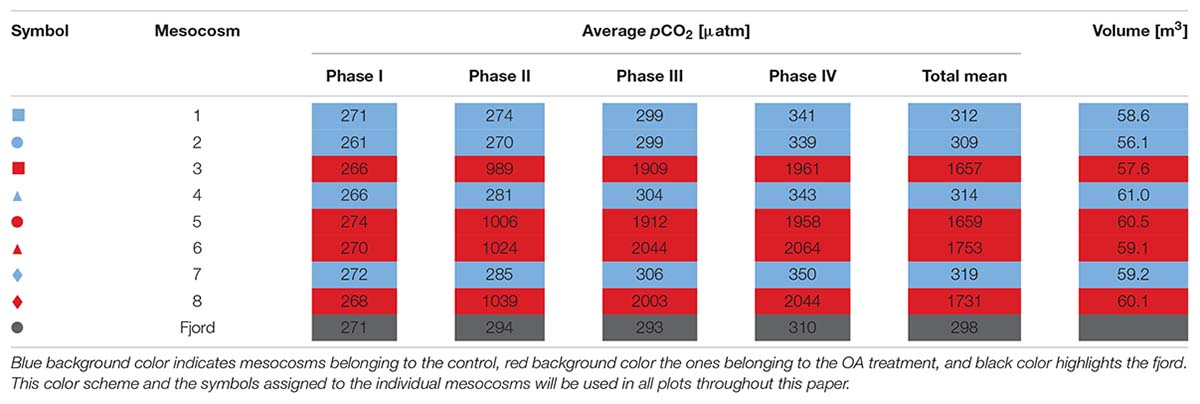
Table 1. Overview of the individual mesocosm numbers, symbols, volumes (section “Volume Determination”), and average pCO₂ values over the four experiment phases (Table 2) and the entire study.

The bottom end of each mesocosm bag is formed by a 2 m long, cone shaped sediment trap, which is attached to lower opening of the bag. This trap is hinged and can be left open or closed with screws. The sediment trap has a steeply angled shape, minimizing adhesive friction of sinking material inside the mesocosm, and leading into a collecting cylinder of ≈3 L volume. A silicon tube for sampling of the accumulated material is attached to the outlet opening of the cylinder and extends to the floating frame of the mesocosm above the sea surface (Boxhammer et al., 2016).

Deployment and Experimental Design

On the 3rd of May 2015 (Day −9, i.e., 9 days before first CO₂ manipulation), eight KOSMOS units were deployed by RV ALKOR. In this process, the mesocosms were arranged in two rows with four mesocosm units per row (M1 – M8, Figure 1C).

After the mesocosms were moored, the initially folded mesocosm bags mounted 1 m below the water surface in the flotation frames were unfolded to a length of 19 m on that same day. During deployment and before mesocosm closure, nets of 3 mm mesh size covered the top and bottom openings of the bags to exclude large and heterogeneously distributed zooplankton (e.g., large adult jellyfish) or nekton (e.g., larger fish) from the enclosures. On the 6th of May (Day −6) mesocosm hoods were installed, and sediment traps were attached by divers at the lower end of the bags. The bottom nets were removed in the morning of the 7th of May (Day −5) and the bags were sealed with the sediment traps at the bottom. Simultaneously, a boat crew pulled the mesocosm bags above the water surface and the upper net was removed, leaving the enclosed water body isolated from the surrounding sea water. The mesocosms were then monitored for 53 days, from the 9th of May (Day −3) until the 30th of June (Day 49) which marked the end of the experiment.

Volume Determination

On the 8th of May (Day −4) the volume of the enclosed water bodies was determined following Czerny et al. (2013). Briefly, a calibrated sodium brine solution was evenly dispersed in each mesocosm, thereby increasing the salinity by 0.2 units. This change in salinity was measured with a conductivity, temperature, density probe (CTD) before and after the addition of the brine solution. The individual mesocosm volumes were calculated from the resulting change in salinity, the amount of brine solution added to the enclosures and the individual seawater density of each mesocosm (for exact volumes see Table 1, for the exact salinity changes see Supplementary Table 1).

CO₂ Addition

To increase pCO₂ in the treatment mesocosms, approximately 1.4 m³ of filtered (30 μm mesh size) fjord water was aerated with pure CO₂ gas for several hours. This CO₂-saturated water was then homogeneously injected into the water columns of the “high pCO₂” mesocosms (M3, M5, M6, and M8) following procedures described in Riebesell et al. (2013a). To treat all mesocosms, similarly, with respect to creating internal turbulences, we also moved the CO₂ injection device up and down in the water columns in the unmanipulated control mesocosms (M1, M2, M4, and M7), but without the addition of any water. The four “high pCO₂” mesocosms were elevated to pCO₂ levels between 2001 μatm (M5) and 2107 μatm (M6) on Day 6 with four initial injections of CO₂-saturated seawater (Day 0, 2, 4, and 6). In the other four “ambient pCO₂” mesocosms the pCO₂ remained similar to the surrounding fjord water with a total average of ≈314 μatm (Table 1). During the experiment, five more CO₂ additions were conducted on Days 14, 22, 28, 40, and 46, to counteract CO₂ losses due to outgassing at the air-sea interface (Figure 2 and Supplementary Table 2).

FIGURE 2

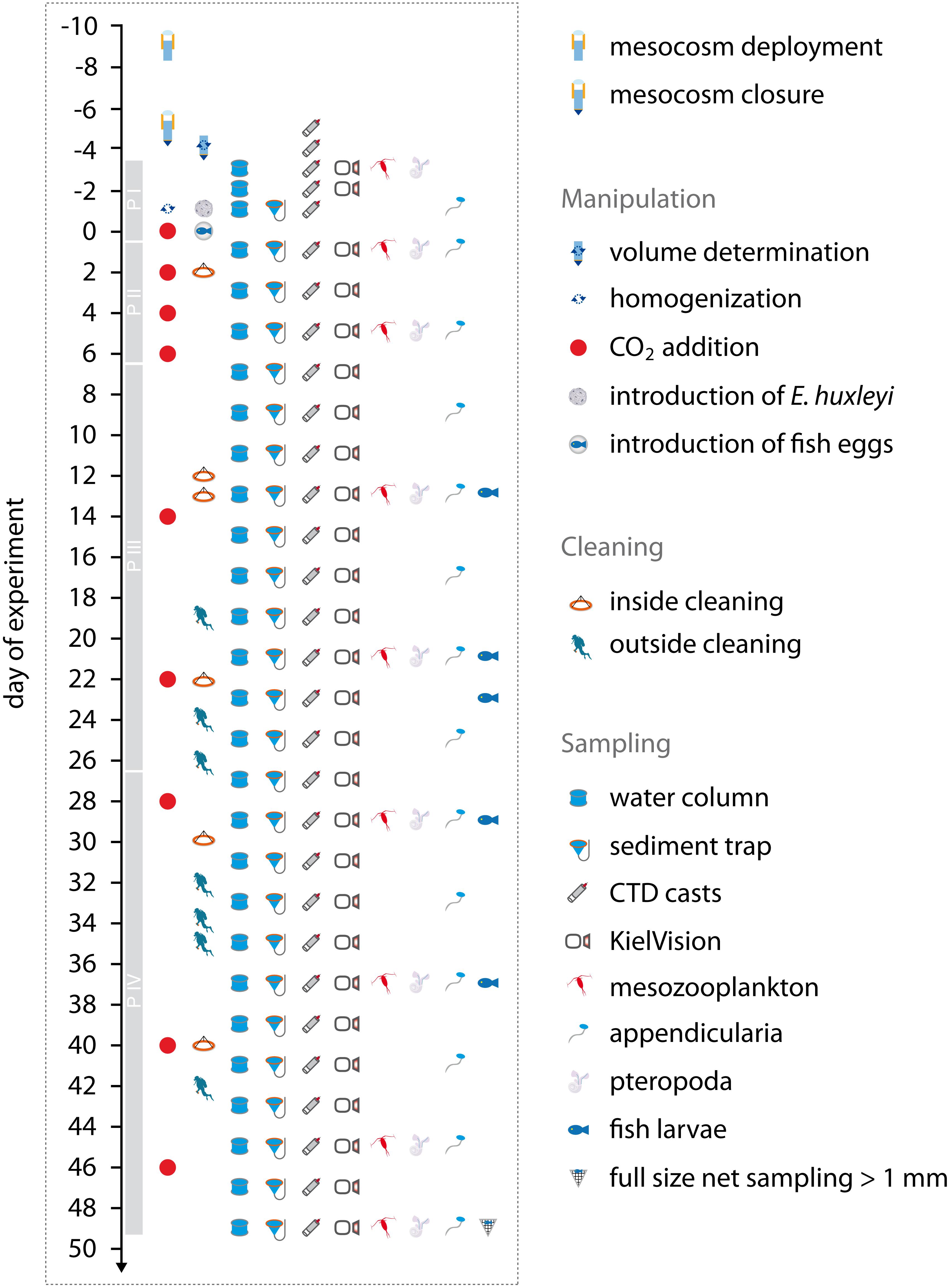
Figure 2. Overview of all sampling and maintenance activities over the course of the experiment, as described in detail in section “Volume Determination”, section “CO₂ Addition”, section “Addition of Organisms to the Mesocosms”, section “Cleaning of Mesocosm Surfaces”, and section “General Sampling Procedure”. Gray bars on the timeline represent the individual phases of the experiment as explained in Table 2. Figure assembled and designed with Adobe Illustrator CS4 (Adobe-Inc, 2008).

According to these time points of the CO₂ additions, and the temporal development of chl a (Figure 4), we divided the experiment into four phases (Table 2). Phase I is thereby characterized as the pre-experimental phase until the first CO₂ addition (Day 0). Phase II is the transitional phase while target pCO₂ levels were established with the four initial CO₂ injections (last addition on Day 6), and the community changed from bloom to post-bloom conditions. Phases III and IV experience post-bloom conditions and were separated to distinguish between an initial temporary treatment effect on chl a (Days 7 to 26), and a second more steady OA effect from Day 27 onward.

TABLE 2

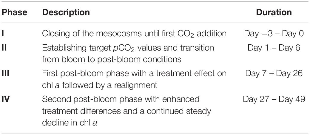
Table 2. Overview, description and duration of the four different phases of the experiment based on pCO₂ additions/manipulations and chl a concentration development.

Addition of Organisms to the Mesocosms

High pCO₂-adapted Emiliania huxleyi

On May 11 (Day −1), a ≈20 L mixture of high pCO₂-adapted (2200 μatm) and ambient pCO₂-adapted Emiliania huxleyi strains was injected evenly into the water column of each mesocosm. The cultures originated from an E. huxleyi strain that was isolated at the exact same location in Raunefjord in 2009. Since 2010, this strain was grown under ambient (400 μatm) and high pCO₂ (2200 μatm) conditions in controlled conditions until this mesocosm experiment in 2015 (for details on culturing and the rationale for the competition experiment between high and ambient pCO₂-adapted E. huxleyi see Lohbeck et al. (2012), Schlüter et al. (2016) and Bach et al. (2018). Both strains were grown in large volumes in the laboratory prior to their addition to the mesocosms. Directly after their injection into the mesocosm, their concentration was ∼100 cells mL^–1. The results of the E. huxleyi competition experiment will be presented in a separate publication.

Atlantic herring larvae

To investigate the influence of extreme OA on higher tropic levels, on average 6364 ± 1257 eggs of the Atlantic herring Clupea harengus (Linné and Salvius, 1758) were added to each mesocosm. From these eggs, on average, 2063 ± 566 larvae hatched in each mesocosm (63 m³). This relates to a herring larval density of 32.7 ± 9.0 larvae per m³ and ∼650 larvae per m². These densities are well within the natural range for nursery grounds with on average 20 larvae per m³, a maximum of 100 larvae per m³ in the Baltic Sea (Oeberst et al., 2009), and 1,000–10,000 larvae per m² along the Norwegian Coasts (ICES, 2007). Furthermore, the number of eggs was chosen to yield enough larvae to ensure sufficient survival until the end of the experiment, but still avoid the risk of a strong top-down effect on the enclosed plankton community. The herring brood stock originated from the Fens Fjord, Norway (approx. 80 km north of the study area) where they were caught at Day −7 and strip-spawned the same day. The fertilized eggs were kept on egg plates in flow-through fjord water until introduction into the mesocosms. On Day 0, the C. harengus eggs were transferred into egg incubators to prevent damage of the eggs, and suspended at 8 m depth in each of the eight mesocosms. From these incubators the larvae could escape freely into the mesocosms right after hatch. The introduction of herring eggs and development of larvae will be discussed in a separate publication.

Cleaning of Mesocosm Surfaces

Inside and outside cleaning of the mesocosm walls was performed at regular intervals to prevent fouling on the mesocosm walls and thus consumption of nutrients and a decrease in light penetration depth. A specifically designed ring-shaped double-bladed wiper was used to clean the mesocosm bags from the inside, while the outside bags were cleaned by divers with scrubbers (Riebesell et al., 2013a; Bach et al., 2016). Only the sediment trap and the last meter of the mesocosm bags could not be cleaned from the inside due to their narrowing diameter and the fixed diameter of the cleaning ring. However, the negative influence of this on light penetration can be considered small, as this is quite deep in the water column (∼18 m below surface).

General Sampling Procedure

A variety of physical, biological, and biogeochemical parameters were measured inside the mesocosms and in the surrounding water at the mesocosm deployment site over the course of the experiment in regular intervals. Before the CO₂-manipulation, from Day −3 until Day −1, sampling was performed daily. Afterward, samples were taken every second day until the end of the experiment (Day 49) (Figure 2). Sampling lasted no longer than 3 h and was always conducted between 8 and 12 am.

Sediment Trap Sampling and Processing

Particles accumulating in the mesocosm sediment traps were removed on each sampling day (Figure 2) before the water column sampling. This was done by using a gentle vacuum pump system as described in Boxhammer et al. (2016). Small subsamples (in total < 10%) were used for particle sinking velocity and respiration measurements as described in Stange et al. (2018). The bulk samples were concentrated by centrifugation, deep frozen at −30°C and then freeze dried for 72 h. The dried bulk samples were ground in a ball mill to a homogeneous powder of 2 – 60 μm particle size and analyzed for biogenic silica (BSi_SED), total particulate carbon (TPC_SED), nitrogen (TPN_SED), and phosphorus (TPP_SED) as described by Boxhammer et al. (2016).

CTD Casts

In order to obtain vertical profiles of temperature, salinity, pH, and photosynthetically active radiation (PAR), a hand-held self-logging CTD probe (CTD60M, Sea and Sun Technologies) was lowered down through the entire water column of each mesocosm and down to 21 m in the surrounding water on every sampling day (Figure 2). Technical details on the sensors and data analysis procedures are described by Schulz and Riebesell (2013). Potentiometric measurements of pH_NBS (NBS scale) from the CTD were corrected to pH_T (total scale) by daily linear correlations of mean water column potentiometric pH_NBS to pH_T as determined from carbonate chemistry measurements [see section “Dissolved Inorganic Carbon (DIC) and Total Alkalinity (TA)”].

Integrated Water Samples

Water samples were taken with a 5 L depth-integrating water sampler (IWS, HYDRO-BIOS, Kiel), controlled electronically via hydrostatic pressure sensors. By constantly sampling water over a defined time (50 mL s^–1) at each depth between 0 and 19 m, the IWS samples represent an average for the defined water column. Subsamples were taken directly from the IWS for those parameters particularly sensitive to gas exchange or contamination. These were: the inorganic nutrients nitrate + nitrite, ammonium, silica, and phosphate [NO₃^– + NO₂^–, NH₄, Si(OH)₄, and PO₄^3–], dissolved inorganic carbon (DIC), total alkalinity (TA), and primary production bioassays [see section “Dissolved Inorganic Carbon (DIC) and Total Alkalinity (TA)” and section “Inorganic Nutrients”)]. Samples for the other parameters (see below) were transferred to 10 L plastic canisters, transported back to the laboratory and stored at in situ water temperature until further processing on the same day. The parameters subsampled from these canisters were: total particulate carbon (TPC), particulate organic carbon (POC), nitrogen (PON), and total particulate phosphorus (TPP), biogenic silica (BSi), chlorophyll a (chl a), phytoplankton pigments, and microscopic counts of phyto- and microzooplankton (analytical procedures described in section “Phytoplankton” and section “Microzooplankton”).

Total Particulate Carbon and Nitrogen (TPC and TPN)

For TPC and TPN, and POC and PON measurements, three replicates of 500 to 1000 mL integrated water samples were filtered (≈200 mbar) through 0.7 μm pre-combusted (450°C for 6 h) GF/F filters. In case the filtration time exceeded 30 min, the vacuum was increased to ≈300 mbar. After filtration, two replicates for TPC and TPN measurements were directly dried at 60°C overnight, while the third filter for POC and PON analysis was fumed with hydrochloric acid (37%) for 2h to remove any particulate inorganic carbon or nitrogen (PIC, PIN) before drying. Subsequently, all filters were packed in tin foil and stored in desiccators until analysis. Measurements were carried out using an elemental CN analyzer (EuroEA) following Sharp (1974). PIC was calculated as the difference between the TPC and POC filters. The vertical flux of TPC_SED and TPN_SED was determined from subsamples of 1–2 mg of the finely ground material from the sediment traps and analyzed as described above for suspended particulate matter.

Total Particulate Phosphorus (TPP)

For TPP, 500 to 1000 mL of IWS water were filtered through 0.7 μm GF/F filters with (≈200 mbar). Until analysis, the filters were stored at −20°C in glass bottles, and immediately preceding the analysis, an oxidizing decomposition reagent (Oxisolv^®, MERCK) was added to each filter. After that, the filters were cooked for 30 min in a pressure cooker, mixed with ascorbic acid and a mix reagent (sulfuric acid + ammonium-heptamolybdate solution + potassium antimonyl tartrate solution), and centrifuged. The absorption of the supernatant was measured at 882 nm in a spectrophotometer. TPP_SED was analyzed from subsamples of 1–2 mg of the finely ground sample material following the same procedure as described for water column samples.

Biogenic Silica (BSi)

For BSi, 500 to 1000 mL of IWS water were filtered through 0.65 μm cellulose acetate filters. The filters were stored at −20°C in closed plastic bottles, and concentrations were determined spectrophotometrically in 1 cm cuvettes at 810 nm, according to Hansen and Koroleff (2007). BSi_SED was also determined from subsamples of 1–2 mg of the processed sample material as described for filters containing particulate matter from the water column.

Dissolved Inorganic Carbon (DIC) and Total Alkalinity (TA)

From a 1500 mL sample taken for carbonate chemistry, 50 and 100 mL subsamples were taken for measurements of DIC and TA, respectively, filtered directly after sampling (0.2 μm prefiltered by syringe, afterward GF/F, 0.7 μm pore size) using a peristaltic pump, and stored at room temperature until measurement on the same day. Great care was taken to avoid gas exchange with the atmosphere in case of the DIC filtrations. DIC concentrations were determined by measuring infrared absorption of triplicate samples using a LI-COR LI-7000 on an AIRICA system (MARIANDA, Kiel). The overall precision was typically better than 5 μmol kg^–1. TA was analyzed by potentiometric titration using a Metrohm 862 Compact Titrosampler and a 907 Titrando unit with a precision <1.5 μmol kg^–1 following the open-cell method described in Dickson et al. (2003). The accuracy of DIC and TA measurements was determined by calibration against certified reference materials (CRM batch 126), supplied by A. Dickson, Scripps Institution of Oceanography (United States). DIC and TA results were used to calculate other carbonate chemistry parameters such as pCO₂, pH (on the total scale: pH_T), calcite (Ω_calcite) and aragonite saturation state (Ω_aragonite). For the calculation we used the Seacarb-R package (Gattuso et al., 2016) with the recommended default settings for carbonate dissociation constants (K₁ and K₂) of Lueker et al. (2000).

Inorganic Nutrients

A total of 250 mL samples for inorganic nutrients were collected in acid-cleaned (10% HCl) plastic bottles (Series 310 PETG), filtered over Whatman 0.45 μm cellulose acetate filters, and analyzed directly after sampling. A SEAL Analytical QuAAtro AutoAnalyzer connected to JASCO Model FP-2020 Intelligent Fluorescence Detector and a SEAL Analytical XY2 autosampler with AACE v.6.04 software were used to measure nitrate and nitrite (NO₃^– + NO₂^–), dissolved silica [Si(OH)₄], and phosphate (PO₄^3–) concentrations spectrophotometrically according to Murphy and Riley (1962) and Hansen and Grasshoff (1983). Ammonium (NH₄⁺) concentrations were determined fluorometrically following Holmes et al. (1999). Refractive index blank reagents were used (Coverly et al., 2012) in order to quantify and correct for the contribution of refraction, color and turbidity on the optical reading of the samples. Instrument precision was calculated from the average standard deviation of triplicate samples (±0.007 μmol L^–1 for NO₃^–/NO₂^–, ±0.003 μmol L^–1 for PO₄^3–, ±0.011 μmol L^–1 for Si(OH)₄, and ±0.005 μmol L^–1 for NH₄⁺). Analyzer performance was controlled by monitoring baseline, calibration coefficients and slopes of the nutrient species over time. The variations observed throughout the experiment were within the analytical error of the methods.

Chl a and Phytoplankton Pigments

After vacuum filtration (<200 mbar) of 250 to 500 mL integrated water samples for chl a and other phytoplankton pigments (0.7 μm GF/F, Whatman), filters were stored in cryovials at −20°C (chl a) and −80°C (pigments) until analysis by reverse-phase high-performance liquid chromatography [HPLC, Barlow et al. (1997)]. For this, all pigments were extracted with acetone (100%) in plastic vials by homogenization of the filters using glass beads in a cell mill. The extract was then centrifuged (10 min, 800^∗g, 4°C), and the supernatant was filtered through 0.2 μm PTFE filters (VWR International). During all these steps the exposure of the samples to light was kept at a minimum. Concentration of phytoplankton pigments was determined by a Thermo Fisher Scientific HPLC Ultimate 3000 with an Eclipse XDB-C8 3.5u 4.6 × 150 column. CHEMTAX software was utilized for classifying phytoplankton based on taxon-specific pigment ratios (Mackey et al., 1996) and calculating the contributions of individual phytoplankton groups to total chl a concentration.

Flow Cytometry

A total of 50 mL subsamples for flow cytometric analysis of phytoplankton were taken from the integrated water samples. From these subsamples, 650 μl per mesocosm were immediately analyzed within 3 h using an Accuri C6 (BD Biosciences) flow cytometer. To verify the flow rate estimated by the Accuri C6, the volume difference of the samples before and after measurement was calculated at regular intervals by weighing. Phytoplankton populations were distinguished based on the signal strength of the forward light scatter (FSC), the red fluorescence from chl a light emission (FL3), and the orange fluorescence from phycoerythrin light emission (FL2) (Olson et al., 1989; Bach et al., 2017).

Primary Production and Photosynthesis Irradiance Response Experiments

To estimate phytoplankton primary production and photophysiology, three 24 h ¹⁴C-uptake primary production experiments on Days −1, 17, and 33, and six 2 h ¹⁴C-uptake photosynthesis-irradiance (P-E) response experiments were conducted on Day −3, 3, 13, 23, 31, and 39 [based on techniques described in Strickland and Parsons (1972); Platt et al. (1980)]. The 24 h primary production experiments (all mesocosms) were carried out in 1 L polycarbonate bottles, at ambient fjord temperature, and ∼30% sunlight attenuated by neutral density screening. The P-E experiments were carried out on a subset of two ambient and two high pCO₂ mesocosms (M1, M3, M7, and M8) in a custom-made photosynthetron in 20 mL borosilicate bottles, at ambient fjord temperature, and ∼15–1500 μmol quanta m^–2 s^–1. All samples were filtered under dim light conditions onto 0.2 μm polycarbonate filters, acidified, measured via liquid scintillation counting (Beckman LS 6000), and dark-corrected. Daily primary production rates for the mesocosm study location were estimated from P-E experiments using 30% of MODIS-Aqua daily averaged estimated photosynthetically available radiation coupled to a daily solar position estimates [as described in Frouin et al. (2012)].

Phytoplankton

To determine phytoplankton abundance, a volume of 250 mL seawater sample was obtained from the IWS water, filled in brown glass bottles, and fixed with acidic Lugol’s iodine (final concentration ≈1%). Phytoplankton counting was performed in settling chambers using an inverted microscope (ZEISS, Germany) according to Utermöhl (1931, 1958); Edler and Elbrächter (2010). Due to high abundances of diatoms at the beginning of the experiment, 50 mL settling chambers were used from Day −3 until Day 5, switching to 100 mL settling chambers thereafter to increase individual counts per species after diatom numbers decreased. Identification was carried out to the species or genus level. See Dörner et al. (2020) for details.

Microzooplankton

For microzooplankton enumeration, 250 mL of seawater sample was taken every 8 days from the IWS water, fixed immediately with acidic Lugol’s iodine solution (final concentration ≈1%), and stored in 250 mL brown glass bottles. Analysis was carried out using the Utermöhl technique (Utermöhl, 1931). See Dörner et al. (2020) for details.

Mesozooplankton

Mesozooplankton (MesoZP) samples were collected from Day −3 every 8 days through vertical net hauls from 19 m depth up to the surface (Figure 2). On every zooplankton sampling day between 11:00 am and 1:00 pm, one net haul was conducted in every mesocosm as well as in the fjord in alternating order, to assure random sampling of the mesocosms between different sampling days. Sampling was carried out using a 100 cm long Apstein net with 55 μm mesh size and a 17 cm diameter cone-shaped opening. This resulted in a sampling volume of 431 L per net haul. The sampling interval of 8 days was chosen in order to minimize the influence on the mesozooplankton community. To get a more detailed overview of the starting conditions in the mesocosms, however, we conducted one additional MesoZP sampling one day after the first CO₂ addition (Day 1). Back in the laboratory, samples were immediately preserved in 70% EtOH. Prior to counting, the samples were split with a Folsom plankton splitter to 1/8 of the original sample. Starting with the first aliquot all organisms larger than 55 μm were counted in a Bogorov-chamber with a Leica stereomicroscope (MZ12) and specified to the lowest possible taxonomic level. Abundant taxa (>50 individuals per aliquot) were only counted from subsamples, while less abundant taxa were counted from entire samples. Zooplankton abundance was calculated assuming 100% filtering efficiency of the net, and abundances were calculated as individuals per m³ (ind m^–3).

Appendicularia

Collection of appendicularians using traditional plankton nets or pumping is too damaging to these fragile gelatinous animals. Moreover, Oikopleura is semelparous organism with a short life cycle, 6 days at 15°C (Bouquet et al., 2009), about 11 days under the mesocosm temperature conditions (Bouquet et al. in prep). Since adult organisms die after reproduction and early stages may also be difficult to detect/identify and account for, abundance continuously varies, between reproduction peak and rise of the next juvenile generation. Hence, to obtain more accurate abundance measurements, it is important to keep the highest sampling frequency permitted by the experimental design and overall mesocosm sampling volume limitation, using an adapted net. Consequently, in addition to the regular MesoZP sampling that also included appendicularia count, an extra net haul was conducted every 4 days (Figure 2). The appendicularia net used during the experiment was designed and adapted to the scale of the mesocosm, in order to collect undamaged specimens, both for abundance quantification down to eggs, embryos and early tadpoles, and culture for parallel additional incubation experiments. The customized net was a 1 m long plankton net with a large cod-end (polycarbonate 3.8 L beaker, diameter of the beaker 17 cm). The opening of the net was 20 cm and the mesh size 55 μm. Vertical tows were manually performed, ∼2 min to lower the net to 18 m and ∼2 min to pull up, corresponding to a lowering and pulling rate of 0.15 m s^–1. For complementary information, technical description, methodology and results of parallel O. dioica laboratory incubation experiments under mesocosm conditions, see Bouquet et al. (in prep).

Hydrozoa

Samples for hydrozoa abundance data were obtained from the regular MesoZP net hauls preserved in 70% EtOH, the four fish larvae net hauls and the final full diameter net sampling (Figure 2). Whenever MesoZP and fish larvae net hauls were conducted on the same sampling day, hydrozoa abundance data was first calculated as individuals per m³ (ind m^–3) for each of the nets, and afterward a mean was taken for calculating the final abundances. To obtain the numbers per net, the entire net samples were scanned under a stereomicroscope (Leica MZ12). Counting of hydrozoa in the fish and final net was performed prior to preservation in 4% phosphate buffered formalin.

Atlantic Herring Larvae

To track the abundance of herring larvae during the experiment, two different methods were applied. First, dead larvae were manually picked out of the sediment trap samples (every second day) to monitor their mortality. Second, four net hauls with a 500 μm mesh size and 50 cm diameter net were performed after sunset on Day 13, Day 23, Day 29, and Day 37 (see Figure 2). Moreover, all herring larvae that survived until the end of the experiment (Day 49) were caught with a full diameter sized net, towed through the entire water column of each mesocosm (1000 μm mesh size, 2 m diameter).

Data Analysis

To analyze whether the OA treatment had a significant influence on the plankton community structure or on biogeochemical parameters of water column and sediment material, we conducted multivariate analyses using the “adonis” function within the “vegan” package in R software version 3.4.2 in the RStudio environment (Rstudio Team, 2016; Oksanen et al., 2019; R Core Team, 2019). This function offers a direct analogous test to Permutational Multivariate Analysis of Variance (PERMANOVA) using distance matrices, and concurrently represents a robust alternative to ordination methods for describing how variation is attributed to different experimental treatments. Overall, this function was applied to plankton community data consisting of averages of the phytoplankton concentrations (μg L^–1, derived from pigment to chl a ratios from HPLC and CHEMTAX), the plankton abundances from microscopic counts of micro- (cells L^–1) and mesozooplankton (ind m^–3), as well as to the concentrations of the water column/sediment biogeochemical core parameters (μmol L^–1). To allow for statistical comparison of these diverse parameters with variable ranges of absolute numbers, the following function for data normalization was applied (1):

$$N_{\mathit{norm}}=\frac{N-N_{\mathit{min}}}{(N_{\mathit{max}}-N_{\mathit{min}})}(1)$$

N_norm is the result of the individual value of the parameter N, divided by the difference between N_max and N_min, being the highest and lowest values for this certain parameter within all mesocosms on a sampling day. These normalized values were averaged according to the treatments and over time within four different phases of the experiment (for description of the phases see Table 2). Before the normalized mean data of every phase of the experiment were tested per phase in the PERMANOVA with regards to the factor pCO₂, every phase-dataset had to be pre-checked for the so called “multivariate spread” among single groups, similar to testing for variance homogeneity in univariate ANOVA. Therefore, the R function ‘betadisper’ as a multivariate analog of Levene’s test for homogeneity of variances was used (Anderson, 2006), and combined with an ANOVA applied to the betadisper result to check for significance. In case the ANOVA returned no significant multivariate spread between the single groups within the dataset, the PERMANOVA could be carried out based on a Bray-Curtis dissimilarity distance matrix. When a significant (p < 0.05) difference between the treatments of one phase was detected, a similarity percentage analysis (SIMPER) was used subsequently to reveal the contributions of the most influential species/parameters to this treatment effect.

For visualization of the results, the mean values per phase where plotted using non-metric multidimensional scaling (nMDS, performed by the metaMDS function from the vegan package in R) based on the same Bray-Curtis dissimilarity distance matrices as used for the PERMANOVA. The nMDS arranges any dissimilarities within the given parameters non-metrically onto an ordination space, where the distance between two points can be used as a hint of the degree of dissimilarity. Additionally, the standard error (SE) and the 95% confidence interval were calculated for every treatment in every phase and implemented as colored ellipsoids in the nMDS plots. The nMDS analysis was only carried out for the plankton data because with the biogeochemistry parameters the analysis provided inconclusive data output due to the low number of input parameters (too high stress values).

The univariate datasets of chl a, primary production, and the different inorganic nutrients were tested for treatment effects by means of a two-sample t-test performed with the R software version 3.4.2 in the RStudio environment. Thereby, a mean of the to-be-examined parameter was calculated per mesocosm per phase, or a certain time frame within a phase, grouped by high and control pCO₂, and tested for significant differences between treatment averages.

Results and Discussion

Temperature and Salinity

Over the course of the experiment the depth-integrated temperature in the mesocosms increased from initially 8.6°C (Day −3) to 10.4°C (Day 49) (Figure 3). Temperature differences between the mesocosms were minimal, around 0.1°C. Warming of the surface layer in the second half of the experiment led to the development of a strong thermocline at about 10 m depth with a temperature decrease of ca. 2°C from 10 m to 15 m. This reflected the natural temperature development in the fjord (Figure 3).

FIGURE 3

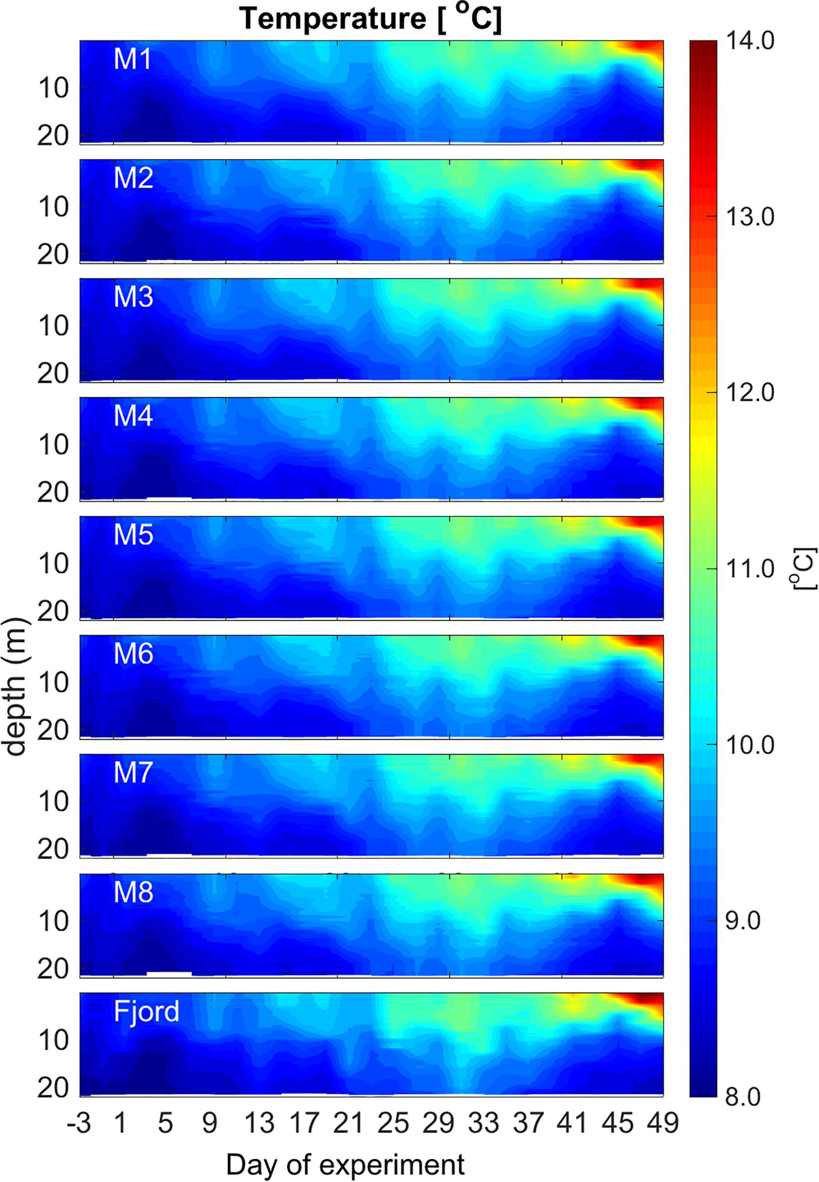
Figure 3. Overview of the CTD – depth profiles of temperature (°C) over the course of the experiment. Figure created with MATLAB (version R2013a).

Regarding salinity, there was no stratification detected inside the mesocosms. Additionally, average salinity of the enclosed water of all mesocosms was nearly constant during the experimental period, with a minor increase of 0.2 from 31.8 (Day −3) to 32 (Day 49) due to evaporation. The salinity in the surrounding water was more variable over time with an average of 31.44 and a halocline shifting between 10 m and 20 m (see Supplementary Figure 1).

Chlorophyll a and Primary Production

Up to the first CO₂ addition on Day 0, the mean chl a concentration was ≈2.2 μg L^–1 (Day 1) in both treatments. It was, therefore, close to the initial values of 2.43 μg L^–1 (±0.24 SD) in the ambient pCO₂ and 2.44 μg L^–1 (±0.16 SD) in the designated high pCO₂ treatment on Day −3. During phase II (Day 0 to Day 6) and early phase III (up to Day 9), chl a decreased quickly to 0.94 μg L^–1 (±0.06 SD) in the ambient pCO₂, and to 0.8 μg L^–1 (±0.09 SD) in the high pCO₂ mesocosms. This decrease was accompanied by a reduced variance within the control and treated mesocosms (Figure 4). From Day 9 onward, the chl a concentration decreased constantly to 0.36 μg L^–1 (±0.03 SD, ambient) and 0.18 μg L^–1 (±0.04 SD, high) until the last day of the experiment, Day 49. Within this period of time, chl a concentration significantly deviated between the treatments during phase III (t-test p < 0.001), and phase IV (t-test p = 0.03). Overall, differences between the treatments were most pronounced on Day 17 with an average chl a concentration of 0.77 μg L^–1 (±0.1 SD) and 0.43 μg L^–1 (±0.02 SD) in the ambient and CO₂-enriched mesocosms, respectively. The difference between initial average chl a concentration in the mesocosms and the fjord (≈2.4 μg L^–1 to ≈3.5 μg L^–1) is most likely a consequence of new water masses entering the fjord with high phytoplankton abundances between the day of mesocosm closure and the first sampling 2 days later (Day −3).

FIGURE 4

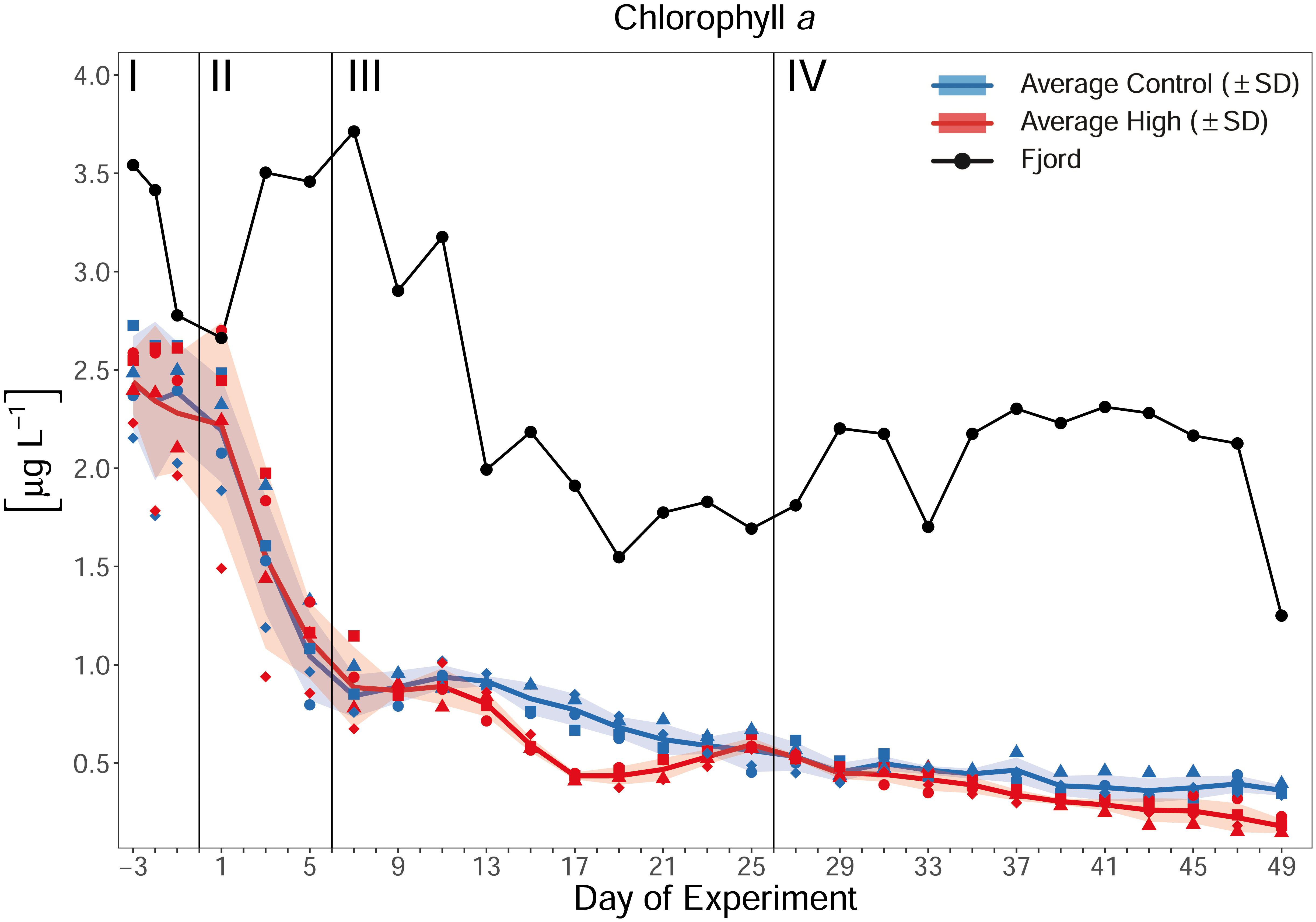
Figure 4. Temporal development of average chl a concentration over the course of the experiment. Blue, red, and black line indicate the respective average concentration in the control, high pCO₂ treatment, and the Fjord. The ribbons represent the standard deviations (SD). Blue symbols represent concentrations in the ambient pCO₂ mesocosms (M1, M2, M4, and M7), red symbols in the high pCO₂ mesocosms (M3, M5, M6, and M8), black symbols represent the fjord. For assignment of symbols to the individual mesocosms see Table 1. Roman numerals indicate the different phases of the experiment separated by vertical lines (for description of phases see Table 2). Figure created with the ggplot2 package in RStudio (Rstudio Team, 2016; Wickham et al., 2016).

Along with the decrease of chl a, the rate of primary production decreased from a mean of 2.01 μmol C L^–1 d^–1 (±0.25 SD) in the control and 1.67 μmol C L^–1 d^–1 (±0.2 SD) in treatment mesocosms on Day −1, to 0.93 μmol C L^–1 d^–1 (±0.18 SD) and 0.92 μmol C L^–1 d^–1 (±0.19 SD) on Day 31 (phase IV, end of measurement), respectively. P^B_max (the light saturated rate of photosynthesis) also decreased, from 3.5 μg C μg chl a^–1 h^–1 (±0.29 SD, control) and 3.32 μg C μg chl a^–1 h^–1 (±0.07 SD, treatment) on Day −3, to 1.09 μg C μg chl a^–1 h^–1 (±0.1 SD, control) and 1.29 μg C μg chl a^–1 h^–1 (±0.25 SD, treatment) on Day 37 (end of measurement). Statistically, primary production and P^B_max measurements display only on Day 17 significantly higher mean values in the ambient mesocosms (t-test, p < 0.05, Supplementary Figure 2).

The observed decreases in chl a, primary production, and P^B_max indicate that the mesocosms were closed during or shortly after the peak of a phytoplankton bloom in the fjord and transitioned into nutrient limited post-bloom conditions, as also supported by inorganic nutrient concentrations (see section “Inorganic Nutrients”). With that, the chl a response to high CO₂ is in line with experiments recently carried out in the Baltic, the Mediterranean, and the North Sea, which suggested a more pronounced ecological impact of OA during low nutrient concentrations (Paul et al., 2015; Bach et al., 2016; Sala et al., 2016). Furthermore, as the mesocosms exclude light in the UV range, the in this study observed negative effect on chl a and primary production might be further enhanced when extrapolating the results to open ocean environments. It was shown by e.g., Gao et al. (2019), that UV radiation can interact with OA, possibly even intensifying a negative OA effect.

Inorganic Nutrients

Along with the late/post bloom temporal development visible in the chl a concentrations, inorganic nutrients decreased and/or stayed low in all mesocosms over the course of the experiment. Dissolved silicate hardly exceeded the detection limit of 0.005 μmol L^–1 with an overall mean of 0.017 μmol L^–1 (±0.015 SD) in the ambient and 0.009 μmol L^–1 (±0.006 SD) in the high pCO₂ mesocosms (Figure 5D), thus indicating silicate limitation for diatoms and other silicifiers. In the bioavailable N pool, neither nitrate and nitrite nor ammonium showed any treatment differences over time. Nitrate and nitrite only took up a higher proportion of the total accessible N in phase I of the experiment, with 0.27 μmol L^–1 (±0.05 SD) and 0.37 μmol L^–1 (±0.13 SD) in the ambient and designated high pCO₂ treatment, respectively. Afterward they decreased until phase IV to means of 0.08 μmol L^–1 (±0.03 SD) in the ambient and 0.09 μmol L^–1 (±0.05 SD) in the high CO₂ mesocosms (Supplementary Figure 3). Compared to ammonium overall mean concentrations of 0.36 μmol L^–1 (±0.12 SD) in the ambient mesocosms and 0.41 μmol L^–1 (±0.18 SD) in the high pCO₂ treatment, most of the accessible N during the CO₂ enrichment and post bloom phases was provided by ammonium as a result of the predominating remineralization processes in the mesocosms. Therefore, the concentrations of nitrate, nitrite and ammonium were combined to a total N concentration (N_Total = NO₃^– + NO₂^– + NH₄⁺) with an overall mean concentration of 0.47 μmol L^–1 (±0.14 SD) in the ambient and 0.54 μmol L^–1 (±0.22 SD) in the high pCO₂ mesocosms (Figure 5A). The same pattern was visible in the phosphate concentrations, but the measured concentrations were low and close to the detection limit. During phase I, PO₄^3– was available with 0.07–0.08 μmol L^–1 in all mesocosms and decreased afterward to 0.04 μmol L^–1 (±0.014 SD) in the control mesocosms and 0.05 μmol L^–1 (±0.006 SD) in the high pCO₂ treatment (Figure 5B). Additionally, the difference in the chl a concentration between Days 13 and 21 (Figure 4) is conversely visible in the phosphate concentration, with a higher concentration in the high pCO₂ treatment between Days 17 and 23 (difference 0.016 μmol L^–1, Figure 5B). The lower chl a concentration in the high pCO₂ mesocosms during this period indicates that a lower phytoplankton biomass led to the lower phosphate consumption compared to the ambient pCO₂ mesocosms. This is furthermore supported by the absences of a treatment separation between Days 17 and 23 in the inorganic N_Total, and a higher N_Total:P ratio in the particulate matter of the mesocosm water column of the high pCO₂ treatment during this time. The lower P consumption of the organisms thereby led to the higher N_Total:P ratio. Together with a steady low inorganic N_Total and an enhanced inorganic P concentration, this resulted in a lower inorganic N_Total:P ratio under high pCO₂, which is, although without statistical significance (SIMPER p = 0.288), visible between Days 13 and 21. The average N_Total:P ratios over the complete experimental period stayed below Redfield [16:1, Redfield et al. (1963)], and fluctuated around a mean of 11.91 (±4.32 SD) in the ambient and 11.73 (±4.51 SD) in the high pCO₂ mesocosms (Figure 5C).

FIGURE 5

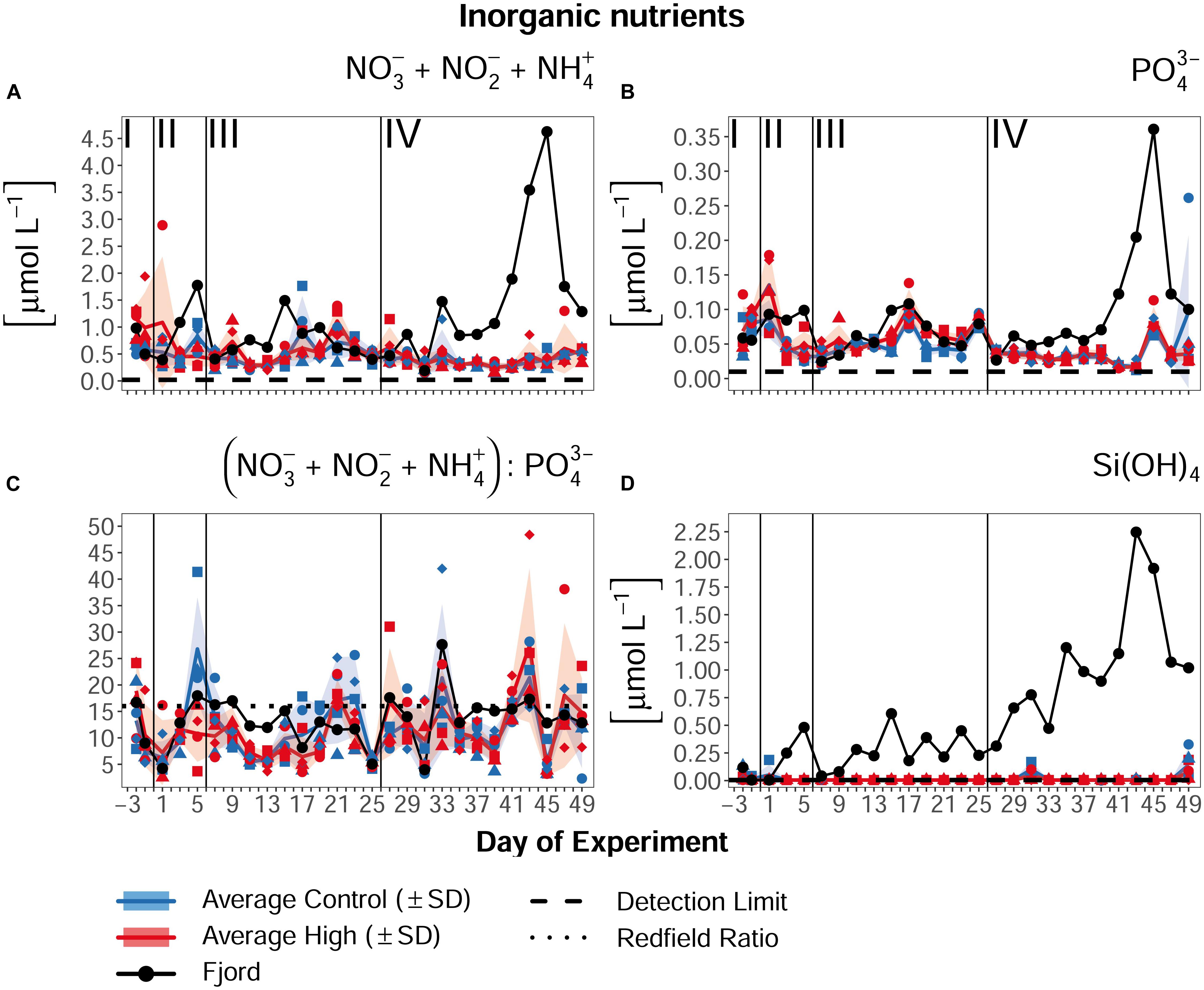
Figure 5. Nutrient concentrations of (A) total N = nitrate + nitrite + ammonium (NO${}_3^{\text{-}}$ + NO${}_2^{\text{-}}$ + NH${}_4^{+}$), (B) phosphate (PO${}_4^{3-}$), (C) total N :P ratio, and (D) dissolved silica Si(OH)₄ over the course of the experiment. Lines, symbols, and colors are used as described in Figure 4. For assignment of symbols to the individual mesocosms see Table 1. Roman numerals label the different phases of the experiment separated by vertical lines (for description of phases see Table 2). Figure created with the ggplot2 package in RStudio (Rstudio Team, 2016; Wickham et al., 2016).

Carbonate Chemistry

Before CO₂-manipulation (phase I), the average pCO₂ in the ambient mesocosms was 271 μatm (±4 SD), and 272 μatm (±4 SD) in the designated high pCO₂ treatment (Figure 6A). Accordingly, average phase I pH_T in all mesocosms was nearly identical, with 8.18 (±0.004) (Figure 6B). Calcium carbonate (CaCO₃) saturation states of calcite (Ω_calcite ≈3.5) and aragonite (Ω_aragonite ≈2.2) exceeded the threshold of 1 in this initial phase.

FIGURE 6

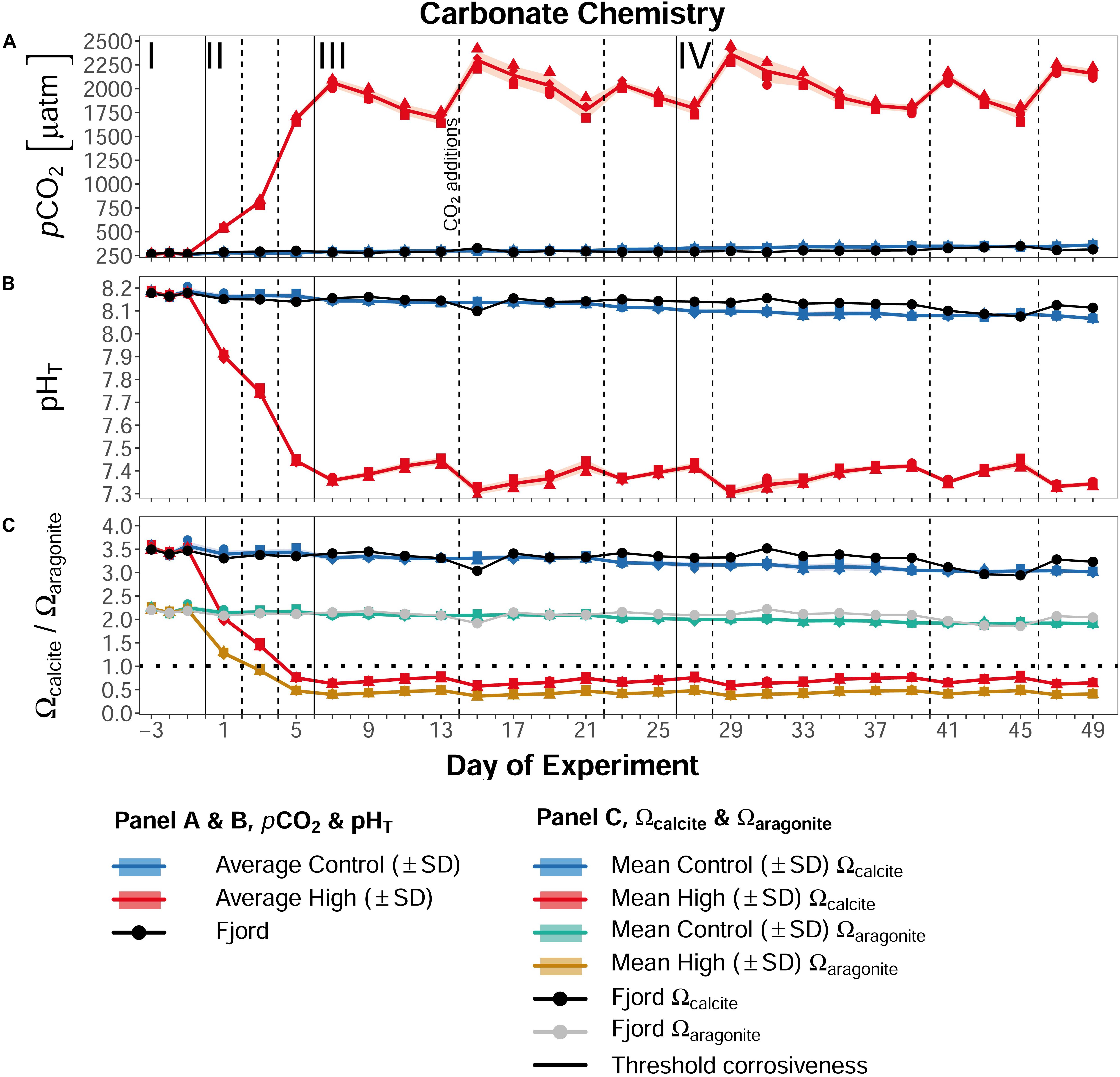
Figure 6. Overview of the carbonate system parameters. (A) Development of the partial pressure of CO₂ in μatm, (B) the pH on the total scale (pH_T), and (C) Ω_calcite (blue and red lines) and Ω_aragonite (green and yellow lines) over the course of the experiment. Lines, symbols, and colors are used as described in Figure 4. Dashed lines indicate CO₂ additions as shown in Figure 2, and described in section “CO₂ Addition.” Roman numerals label the different phases of the experiment separated by vertical lines (for description of phases see Table 2). Figure created with the ggplot2 package in RStudio (Rstudio Team, 2016; Wickham et al., 2016).

From Day 0 on, the stepwise CO₂ additions increased the pCO₂ of the high treatment from initially 271 μatm to on average 553 μatm (±20) on Day 1, 821 μatm (±30) on Day 3, 1690 μatm (±30) on Day 5, and 2069 μatm (±50) on Day 7. As a result of this increase in pCO₂, the pH_T of the high pCO₂ mesocosms decreased to 7.36 (±0.01), and Ω_calcite and Ω_aragonite both dropped below 1 (≈0.6 and ≈0.4, respectively), leading to corrosive conditions for CaCO₃. Due to repeated CO₂ additions (see section CO₂ addition) the extreme pCO₂ conditions in the CO₂-enriched mesocosms were maintained througout the experiment, with phases III and IV means of 1978 μatm (±60) and 2012 μatm (±50), respectively. In the control mesocosms, the pCO₂ increased over the course of the study due to rising water temperature and ingassing of atmospheric CO₂ from initially 271 μatm (±4, phase I), to 365 μatm (±5) on Day 49. Consequently, the pH_T decreased by about 0.1 unit to 8.07 (±0.01), and Ω_calcite and Ω_aragonite declined to ≈3.0 and ≈2.0, respectively. Similar changes in the carbonate chemistry were also observed in the surrounding fjord water (Figure 6).

Effects of High pCO₂ on the Plankton Community

To examine the effects of high pCO₂ levels and the related changes in seawater carbonate chemistry on the post-bloom plankton community, we analyzed the composition and succession patterns of the phytoplankton, micro-, and mesozooplankton communities during the different experimental phases. The analysis was performed from a whole-community perspective, rather than considering single-species responses. More detailed analyses of individual phyto-, microzoo-, and mesozooplankton groups and species will be provided in separate studies that are in preparation.

Phase I

During the first phase, the PERMANOVA did not reveal significant differences of the plankton community composition between the control and the high pCO₂ treatment [P(perm) = 0.113]. The corresponding non-metric multidimensional scaling (nMDS) plots for phase I supports this result (Figure 7I), and is with a stress value of 0.08 considered a reliable depiction of the multivariate dataset. Additionally, the overall small spread of data/response variables of both, high and control pCO₂ mesocosms in the chosen two-dimensional space indicates that the plankton community composition of the mesocosms was overall similar. Nevertheless, the mesocosms displayed a tendency to ordinate according to their designated treatment which can be explained by SIMPER analysis. The test identified a significantly elevated average chl a concentration related to increased numbers of Cyanophyceae (“Cyano”, μg L^–1) in the high pCO₂ treatment, slightly separating the mesocosms in the two-dimensional space.

FIGURE 7

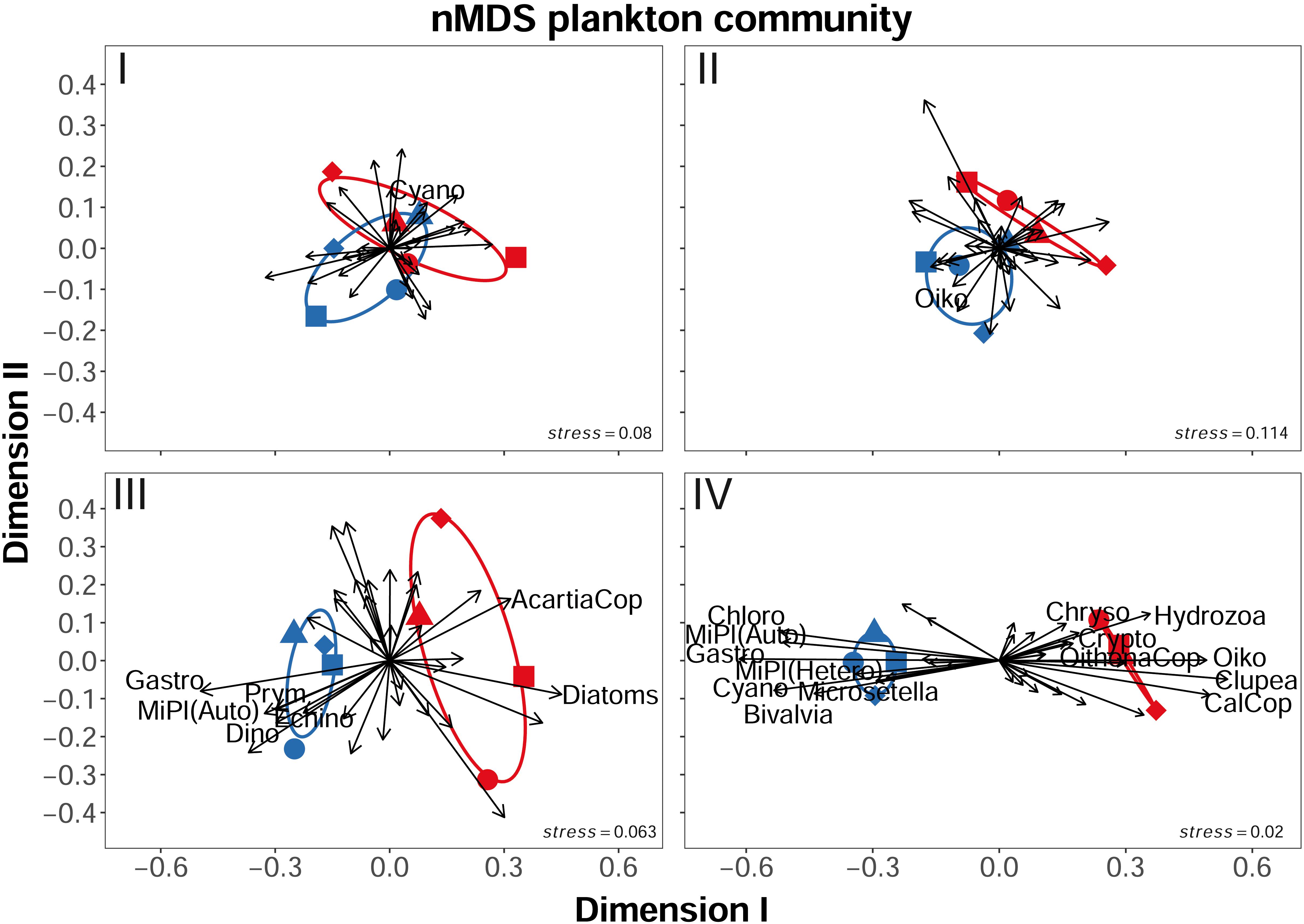
Figure 7. Non-metric dimensional scaling (nMDS) plots of range normalized mesocosm plankton community data for the different phases of the experiment. (I) The initial phase before CO₂ addition. (II) Establishing of target pCO₂ values and transition from bloom to post-bloom conditions. (III) First phase of post-bloom conditions and treatment effect. (IV) Final post-bloom phase. Stress values indicate how accurate dissimilarities among plankton communities in the mesocosms are depicted, arrows indicate the role of the various plankton groups for spatial organization of the mesocosms. AcartiaCop = Acartia spp. copepodites, CalCop = Calanus spp. copepodites, Chloro = Chlorophyceae, Chryso = Chrysophyceae, Clupea = Clupea harengus larvae, Crypto = Cryptophyceae, Cyano = Cyanophyceae, Diatoms = Bacillariophyceae, Dino = Dinophyceae, Echino = Echinodermata larvae, Gastro = Gastropoda larvae, MiPl (Auto) = autotrophic microplankton, MiPl (Hetero) = heterotrophic microplankton, OithonaCop = Oithona spp. copepodites, Oiko = Oikopleura dioica, Prym = Prymnesiophyceae. Figure created with the ggplot2 package in RStudio (Rstudio Team, 2016; Wickham et al., 2016).

Phase II

The treatment separation indicated in phase I developed even further during the acidification process in phase II of the experiment, resulting in a significant split-up of the mesocosms according to their treatment [P(perm) = 0.032]. However, SIMPER identified only one significant influence to this separation, being higher abundances of the appendicularian Oikopleura dioica (“Oiko”, ind m^–3) in the control mesocosms. This is well illustrated by the phase II nMDS plot (Figure 7II, stress = 0.114). Although the mesocosms are still overall close together, their “within treatment” internal variation is reduced, and in combination with the significant effect on O. dioica, a visible separation is caused.

Phase III

With the pCO₂ manipulation fully established in phase III, the significant difference between the plankton communities of the control and the treatment mesocosms got more pronounced [P(perm) = 0.028, Figure 7III]. The SIMPER analysis revealed that 7 different taxa accounted for 36.2 % of the detected difference between the treated and the control mesocosms (p = 0.026). The most influential taxa in this context were Gastropoda (“Gastro”, ind m^–3), Prymnesiophyceae (“Prym”, chl a μg L^–1, mainly Coccolithophoridae, i.e., E. huxleyi), Dinophycaea (“Dino”, chl a μg L^–1), and Echinodermata (“Echino”, chl a μg L^–1), all with negative responses in abundance to the extreme OA level (see Supplementary Table 3). Positive responses to OA in this phase were observed for diatoms and Acartia spp. copepodites. Furthermore, the significant contribution of gastropods, echinoderms, autotrophic microplankton [“MiPl(Auto)”], and copepodites of Acartia spp. (“AcartiaCop”) to the treatment separation emphasizes that OA did not only influence the primary producers in this study but also to a large extent the mesozooplankton (MesoZP) community. In the corresponding nMDS plot (stress: 0.063) this becomes apparent as an obvious separation of the high pCO₂ treatment and the control in the ordination space following the effects on those taxa (see Figure 7III).

Interpretation of observed CO₂ effects during phase III

The negative effect on calcifiers (here Gastropoda) is well in line with previous studies (Lischka et al., 2011; Wittmann and Pörtner, 2013), and reflects the well-studied mechanism of lower calcification rates and/or CaCO₃ dissolution due to the low carbonate saturation states under high pCO₂-levels. The effects of high pCO₂ on echinoderms are variable, as studies with comparable durations and pH values revealed both negative and positive OA effects on factors like growth rate, calcification, and survival (Dupont et al., 2010). This is consistent with our results, which showed an initial negative impact on echinoderms in phase III, and no detectable effect in phase IV (Figure 7IV). This suggests that the treatment effect on echinoderm larvae abundances in phase III could have been triggered indirectly via food availability and not necessarily directly by high pCO₂ impacts on the organism’s physiology. The same can be assumed for the observed positive treatment effect on the abundances of Acartia spp. copepodites. A direct response to these OA levels would more likely be a negative one, as Zhang et al. (2011) found a negative response of Acartia spinicauda at a similar pCO₂ level of 2000 μatm, and Cripps et al. (2014) detected decreasing numbers of Acartia tonsa nauplii already at 1000 μatm. However, these experiments were carried out under controlled laboratory conditions, and did not account for complex changes in a natural food web. Nevertheless, within a natural community influenced by such an extreme level of OA, the indirect positive effect on Acartia spp. copepodites observed in this study is not consistent with previous findings. For example, Niehoff et al. (2013) (pCO₂ up to 1420 μatm) and Hildebrandt (2014) (pCO₂ up to 3000 μatm) studied Acartia spp. under elevated pCO₂ conditions in comparative mesocosm experiments but did not observe any significant effects. This large variability of CO₂ effects points toward the importance of food-web structure and related trophic cascades in determining the response of zooplankton to OA.

Phase IV

The nMDS plot of the second post-bloom period (phase IV) suggests that dissimilarities between the control and treatment mesocosms (stress: 0.02) further increased during this phase. The two-dimensional space separating control and treatment from each other increased and the internal variability within the treatments decreased (Figure 7IV). Consistent with this visual impression, the PERMANOVA of phase IV plankton data revealed a significant treatment effect [P(perm) = 0.028] and the subsequent SIMPER analysis yielded 14 planktonic taxa that accounted for ≈55% of the observed dissimilarities (p = 0.03). The four most influential taxa were Chlorophyceae (“Chloro”), Cyanophyceae (“Cyano”), Gastropoda (“Gastro”, mostly veliger larvae), and appendicularians (“Oiko”, represented by the species Oikopleura dioica), as also indicated by arrow orientation and length in the associated nMDS plot. Compared to phase III, the contribution of mesozooplankton taxa to the treatment dissimilarities increased from 43% (3 out of 7) to 57% (8 of 14) in phase IV. While we found negative effects on the abundance of calcifying organisms (Gastropoda and Bivalvia larvae), autotroph and heterotroph protists, and the copepod Microsetella spp. (“Microsetella”), positive effects of OA were visible in the abundances of all the remaining MesoZP taxa: Oithona spp. copepodites (“OithonaCop”), Calanus spp. copepodites (“CalCop”), O. dioica, hydrozoa, and the abundance of Clupea harengus larvae (“Clupea”) (see Supplementary Table 3).

Interpretation of observed CO₂ effects during phase IV

The fact that elevated pCO₂ levels can alter phytoplankton communities to the advantage or disadvantage of the inherent taxa was already shown in a variety of studies (Dutkiewicz et al., 2015). Furthermore, the specific response of a certain region or plankton community strongly depends on the predominant environmental conditions and community composition. Under the given complexity of the enclosed plankton community, it is challenging to distinguish between direct and indirect pCO₂ effects. An example for the possible mixture of both is the negative effect on Cyanophyceae observed in phase IV. In a comparable mesocosm study, Bach et al. (2017) observed negative as well as positive effects on Cyanophyceae under elevated pCO₂ (760 μatm), and stated that it was most likely an indirect food web effect, although they could not exclude the possibility of a direct CO₂ effect. Apparently easier to determine is the here observed negative effect on Prymnesiophyceae, most likely being a direct effect on the calcifier E. huxleyi in this group. This direct negative effect on Prymnesiophyceae was also confirmed under different elevated pCO₂ scenarios (ranging from 700 to 3000 μatm) in different large scale mesocosm experiments (Engel et al., 2008; Hopkins et al., 2010; Riebesell et al., 2017) as well as at an Antarctic coastal site (Thomson et al., 2016). As already discussed for the results of phase III, positive or negative effects on copepods depend to a large degree on trophodynamic interactions and community composition. However, in contrast to the present study, most experiments do not account for indirect food web effects that may occur in natural communities. As already pointed out for the positive treatment effect on Acartia spp. in phase III, a direct positive effect of OA on the MesoZP taxa in phase IV seems unlikely. Calanus spp. were generally observed to be able to tolerate pCO₂ values >3000 μatm (Weydmann et al., 2012; Hildebrandt, 2014) without effects on survival, hatching success or egg production. Younger stages of Oithona spp. were reported to be more sensitive to OA regarding their growth rate and survival (Lewis et al., 2013; Pedersen et al., 2014), but mesocosm studies by Niehoff et al. (2013) and Hildebrandt (2014) did not find any OA treatment effect on either of these species. On the other hand, experiments by Harris et al. (2000) and Søreide et al. (2008) revealed that diatoms and Cryptophyceae, both of which were positively influenced in phases III and IV of our experiment, make up the main prey of Calanus spp. This enhanced food availability could indirectly have supported the positive responses of Calanus spp. and Oithona spp. in the high pCO₂ mesocosms, which then in turn indirectly could have triggered the positive response of Hydrozoa in the manipulated mesocosms. A direct effect on Hydrozoa in this context is unlikely, as there is currently no scientific work known to the authors that suggests the possibility of a direct positive CO₂ effect. So far, it is rather suspected that there is a direct negative CO₂ effect on the jellyfish balance sensory receptors made of basanite (Werner, 1993). The observed positive effect on O. dioica abundances, however, is very likely a direct OA effect. It was shown by Bouquet et al. (in prep) with parallel incubation experiments using specimens and water from the mesocosms during our study, that the fecundity of O. dioica was significantly higher under high pCO₂ (334 ± 140 eggs) compared to low pCO₂ (278 ± 107 eggs, ANOVA: F(1,6) = 8.60; p = 0.0262). A result that was already observed in other laboratory and mesocosms studies, although not investigated under such extreme pCO₂ conditions (Troedsson et al., 2012; Winder et al., 2017; Bouquet et al., 2018).

Hypothesis (1): Plankton community composition/structure will change under extreme pH values.

Our first hypothesis can be confirmed. We observed an overall restructuring of the plankton community under high pCO₂ on multiple trophic levels of the food web, ranging from primary producers to herbivorous and carnivorous consumers. Besides direct negative OA effects on calcifying organisms like Gastropoda, Bivalvia, and Prymnesiophyceae (mainly Coccolithophoridae), indirect effects via the food web were the main drivers of the significant OA treatment separation (see Figure 10). In this context, positively affected Bacillariophyceae and Cryptophyceae, inter alia, triggered higher abundances of Calanus spp., Oithona spp., and Acartia spp., probably supporting an increase of Hydrozoa and Clupea harengus larvae (Figure 10). Together with higher numbers of filter feeding appendicularians, this led to a substantial increase of top-down control in the food web.

Effects of High pCO₂ on Biogeochemistry

In order to examine how the observed restructuring of the plankton community influenced the biogeochemical cycling in the enclosed water bodies, suspended particulate carbon, nitrogen, phosphorus, and biogenic silica concentrations (μmol L^–1) as well as the respective vertical flux of these elements collected in the sediment traps (μmol L^–1 48 h^–1) were analyzed.

Phase I and II

In phase I as well as during the transition from bloom to post-bloom conditions in phase II, PERMANOVA and SIMPER analysis did not uncover a significant difference between the ambient and high pCO₂ mesocosms in any of the POM parameters in the water column (POM_WATER) or in the collected sediment trap samples (POM_SED) [phase I: P(perm) = 1.0000, phase II: P(perm) = 0.5966]. The mean POC_WATER value of the designated treatment mesocosms was 19.95 μmol L^–1 (±1.33 SD) in phase I, and 20.42 μmol L^–1 (±0.99 SD) during the acidification phase II, while the control mesocosms had POC_WATER values of 20.84 μmol L^–1 (±1.31 SD), and 20.71 μmol L^–1 (±1.39 SD), respectively (Figure 8A and Table 3). Accordingly, there was no treatment effect visible in the related POC_WATER:PON_WATER ratios in phases I and II (Figure 9A). The POC_SED:PON_SED ratio in phase II showed a slightly increasing trend (Figure 9B), and was in the high pCO₂ treatment as well as in the control, higher than the water column ratios (Table 3). This indicates that the emerging nutrient limitation lead to the preferential remineralization of N over C, as already observed for example by Stange et al. (2018) or Schneider et al. (2003). Furthermore, the stable or even slightly increasing concentrations of POC_WATER in combination with the decreasing POC_SED flux (Figures 8A,B), and the sharp decrease of chl a (Figure 4) and primary production in phase II suggest that the biomass of the fading bloom was retained in the water column, i.e., being efficiently recycled by heterotrophs and/or consumed by mesozooplankton, hydrozoans or fish larvae.

FIGURE 8

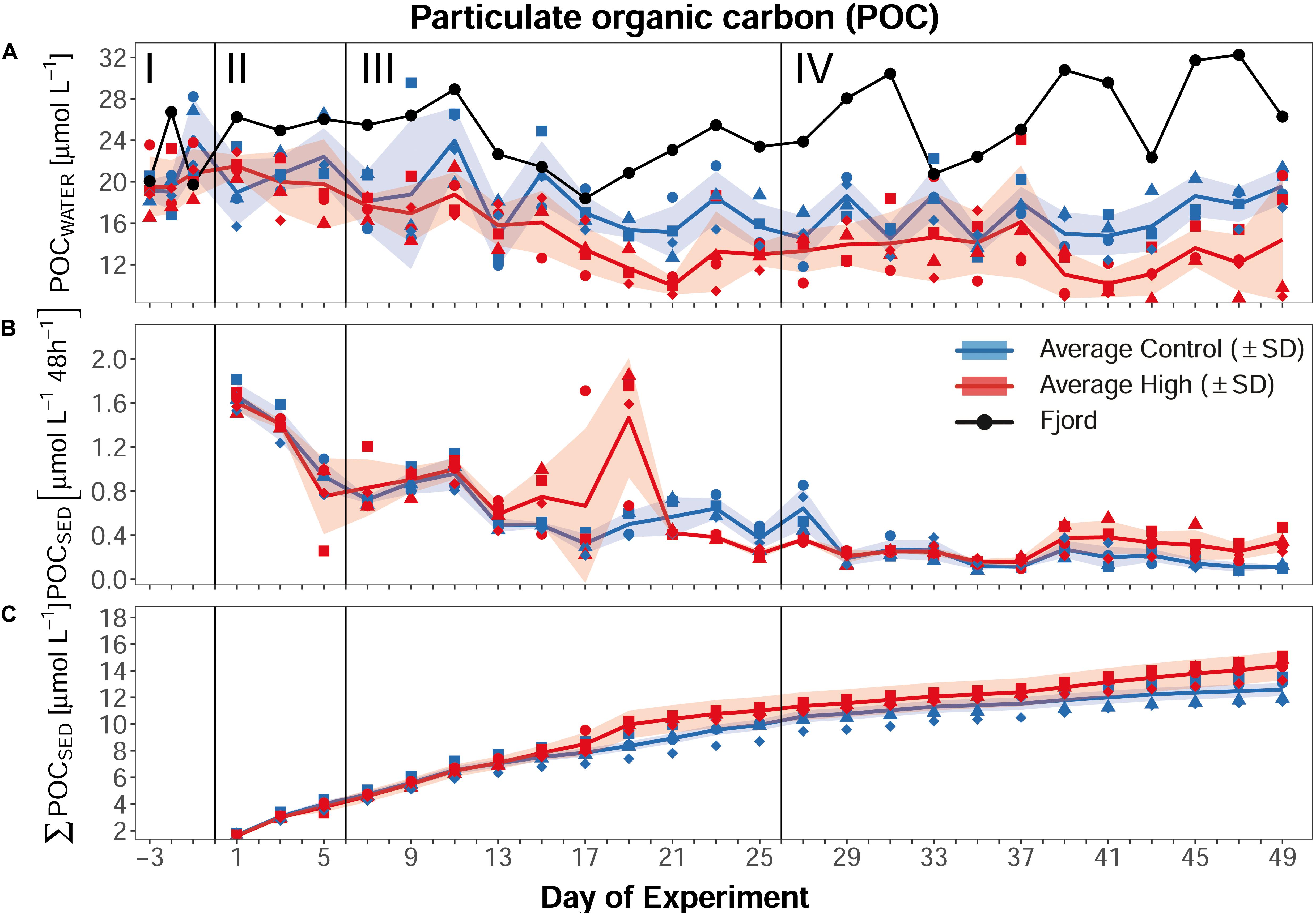
Figure 8. Overview of particulate organic carbon (POC) concentrations and vertical fluxes. Development of (A) POC concentration within the water column (B) the 48 h POC flux collected in the sediment traps, and (C) the cumulative vertical POC flux over the course of the experiment. Lines, symbols, and colors are used as described in Figure 4. Roman numerals label the different phases of the experiment separated by vertical lines (for description of phases see Table 2). Figure created with the ggplot2 package in RStudio (Rstudio Team, 2016; Wickham et al., 2016).

TABLE 3

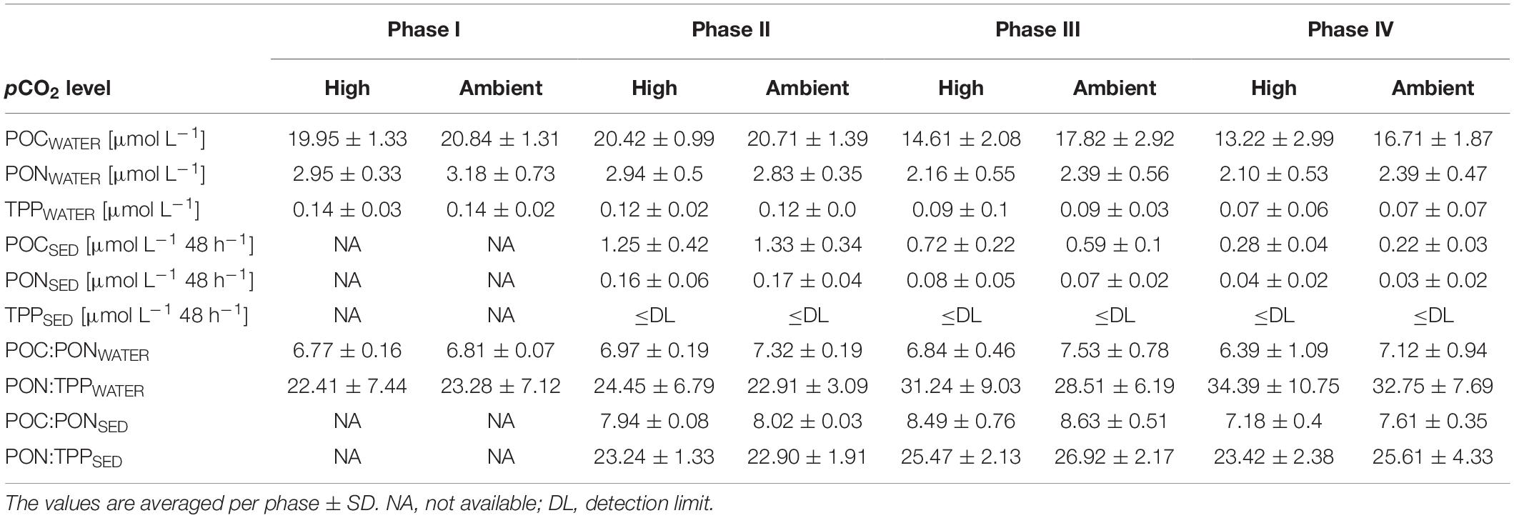
Table 3. Summary of average POM_WATER, and POM_SED values as well as their elemental ratios under the different pCO₂ levels and the four phases of the experiment.

FIGURE 9

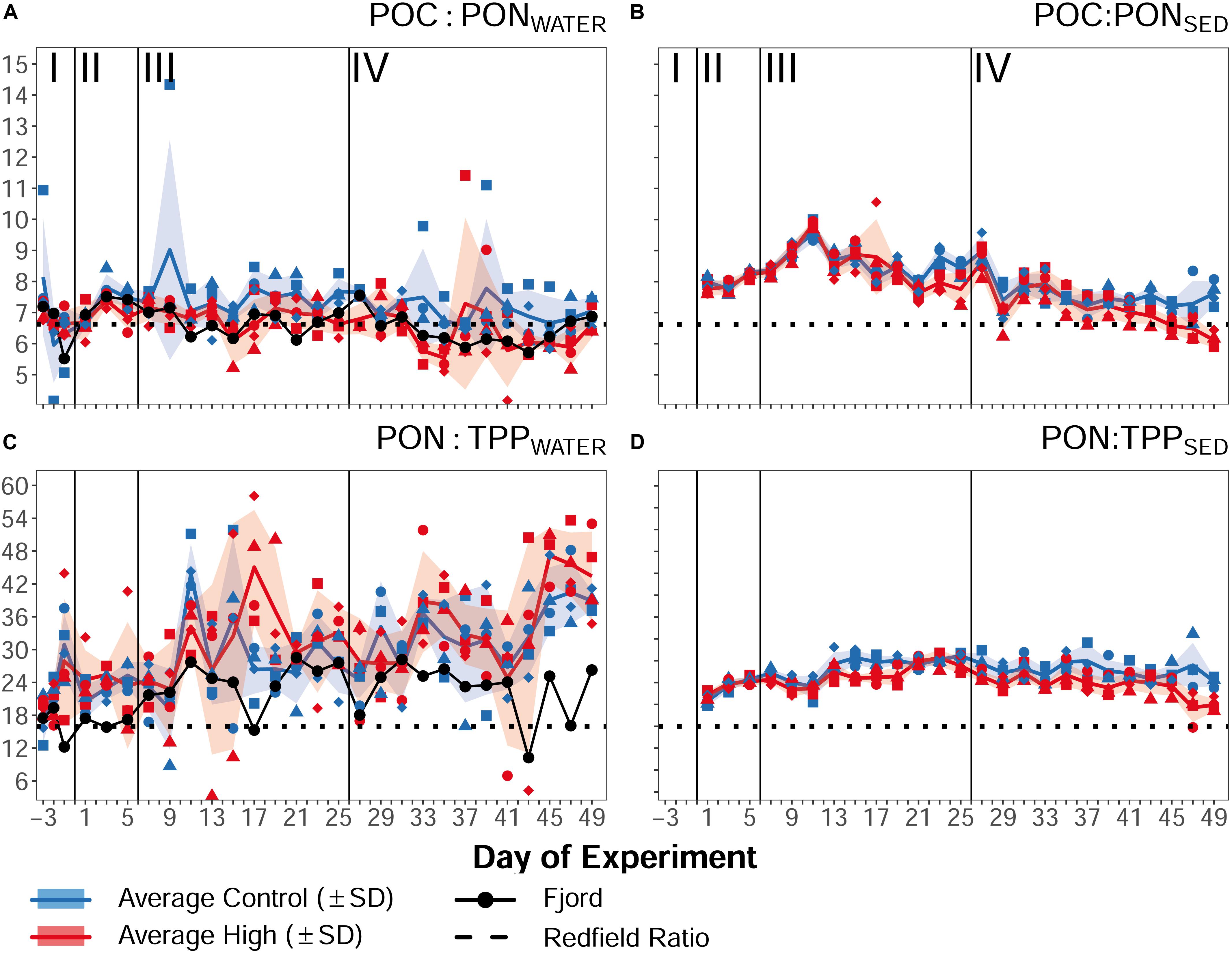
Figure 9. Organic matter ratios of (A) particulate organic carbon and nitrogen in the water column, (B) the respective flux to the sediment trap, (C) particulate organic nitrogen and particulate phosphorous in the water column, and (D) the respective flux to the sediment trap over the course of the experiment. Lines, symbols, and colors are used as described in Figure 4. Roman numerals label the different phases of the experiment separated by vertical lines (for description of phases see Table 2). Figure created with the ggplot2 package in RStudio (Rstudio Team, 2016; Wickham et al., 2016).

FIGURE 10

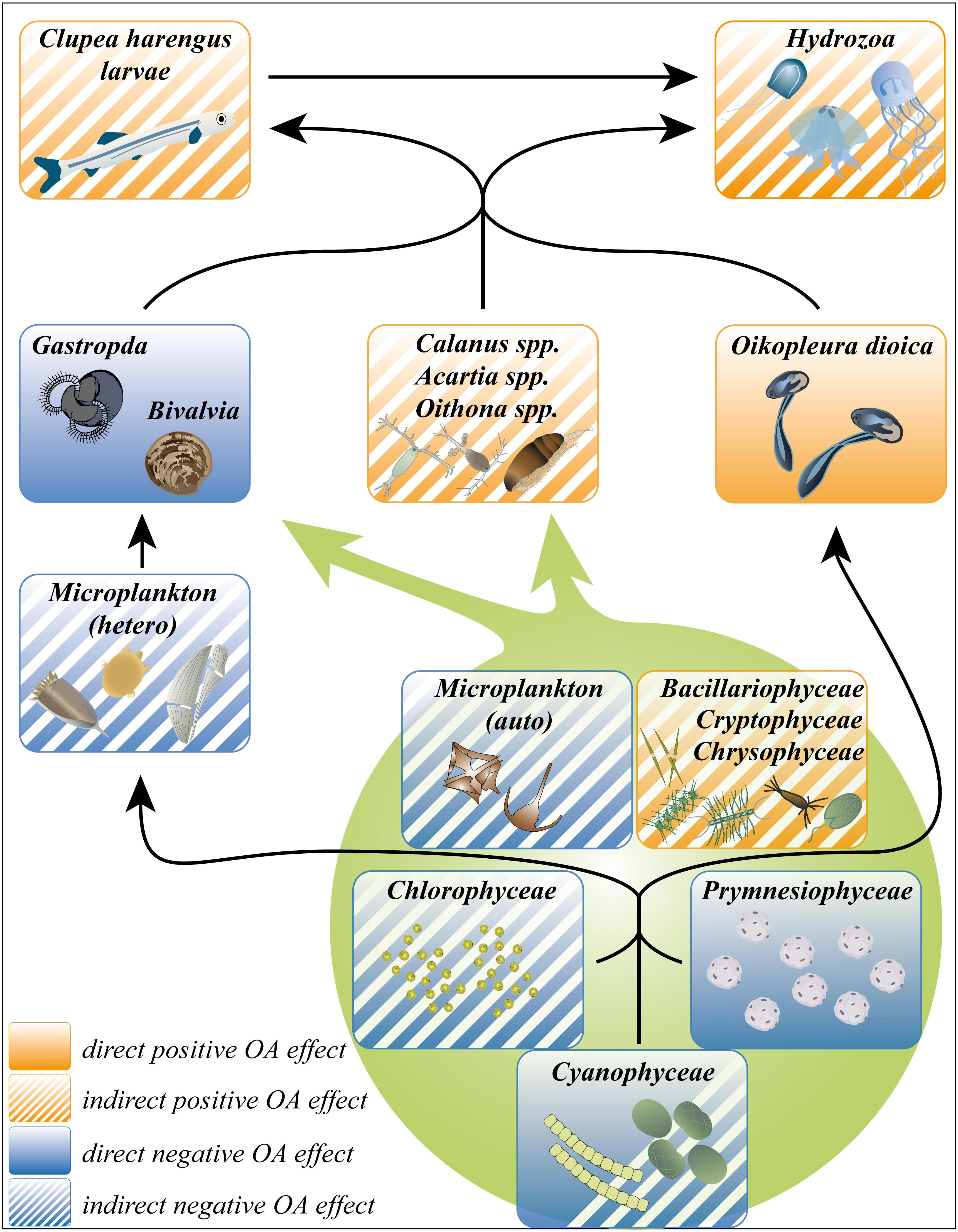
Figure 10. Overview over the positive and negative, direct and indirect OA effects within a simplified food web of our high pCO₂ treatment mesocosms. Squares containing a mixture of filled and hatched area indicate both direct and indirect OA effects on the contained taxa. Black arrows indicate the direction of biomass transfer due to the predator-prey relationships between the single taxa. Green circle summarizes all affected phytoplankton taxa. Symbols taken from “Courtesy of the Integration and Application Network, University of Maryland Center for Environmental Science (ian.umces.edu/symbols/)”, accessed 25.08.2020; Figure design Susanne Schorr, assembled and designed with Adobe Illustrator CS4 (Adobe-Inc, 2008).

Phase III

In phase III, a significant difference between ambient and high pCO₂ mesocosms was observed in POM_WATER data by PERMANOVA [P(perm) = 0.031], which coincides with the emergence of significant CO₂ effects on the plankton community composition. The similarity percentage analysis did not identify any effect on one of the POM_SED parameters, but revealed a significant negative effect on POC_WATER, TPP_WATER, and PON_WATER as major factors for the difference between the control and the treatment (p = 0.032). POC_WATER decreased further during phase III in both ambient and high pCO₂, but in comparison concentrations stayed higher in the ambient pCO₂ mesocosms (Figure 8A and Table 3). The opposite was found in the POC_SED flux (see Figure 8B and Table 3), indicating that carbon export was temporarily enhanced under high pCO₂ conditions. POC_WATER:PON_WATER was not significantly different between the high and ambient pCO₂, but both exceeded the Redfield Ratio (6.6, Figure 9A and Table 3). The PON_WATER:TPP_WATER ratio increased over time but displayed no treatment differences (Figure 9C and Table 3). POC_SED:PON_SED ratio of sinking particles increased in the first half of phase III (until Day 11, Figure 9B), and then decreased sharply to 8.80 (±0.31 SD) under ambient pCO₂ and 7.94 (±0.28 SD) in the high pCO₂ mesocosms. Subsequently, ambient and high pCO₂ start to deviate until the end of phase III with 7.76 (±0.47 SD) in the high pCO₂, and 8.43 (±0.24 SD) in the ambient pCO₂ mesocosms on Day 25. As already observed in phase II, the POC_SED:PON_SED ratio was higher, and the PON_SED:TPP_SED lower than the respective ratios in the water column, indicating preferential remineralization of N over P and C.

Phase IV

The high pCO₂ treatment effect continued in phase IV at a comparable scale. The PERMANOVA result was significant [P(perm) = 0.027], and SIMPER revealed the same major contributing parameters POC_WATER, and TPP_WATER (p = 0.029), albeit with a lower percentage contribution on the treatment differences (≈38% compared to ≈48% in phase III). POC_WATER concentration in this phase was significantly higher in the ambient pCO₂ mesocosms than under high pCO₂ conditions (see Figure 8A and Table 3). As in phase III, SIMPER does not point toward any of the export flux parameters to drive the treatment differences, with a similar average POC_SED between ambient and high pCO₂ treatment (Figure 8B and Table 3). The cumulative ΣPOC_SED data, however, supports the observed OA treatment effects in POM_WATER. In accordance with the significant negative effect on the concentration of POC_WATER, the cumulative mean ΣPOC_SED flux increased in the high pCO₂ treatment from 4.59 μmol L^–1 (±0.44 SD) at the beginning of phase III to 14.38 μmol L^–1 (±1.08 SD) at the end of phase IV (see Figure 8C). Compared to the ambient pCO₂ mesocosms, this led to a final treatment difference of 1.8 μmol L^–1 on Day 49 (ambient pCO₂: 12.58 μmol L^–1 ± 0.49 SD).

Hypothesis (2): Extreme pH will accordingly (along with the plankton community changes) influence the biogeochemistry in the enclosed ecosystem.

Our observations of OA effects on biogeochemical parameters in phases III and IV along with the consistent treatment differences already observed in chl a, lead to the confirmation of our second hypothesis. The reduced phytoplankton biomass in the high pCO₂ treatment was also seen in POM_WATER concentrations. Reduced POM_WATER, in turn, was reflected in higher POM_SED export flux. This could suggest that POM was less efficiently recycled in the high pCO₂ treatment. Alternatively, when considering the already observed restructuring of the MesoZP-community, the higher mean export flux of POM_SED in the high pCO₂ treatment in phases III and IV could be driven by the positive OA effects on zooplankton abundances. In this case, the lower concentrations of chl a and POM_WATER under high pCO₂ could be explained with more dominant top-down control. Indeed, grazing pressure on phytoplankton may have been sufficient to directly transfer any new production to higher trophic levels. This hypothesis of a stronger top-down controlled community in the high pCO₂ treatment leading to higher export flux seems likely if one considers the positive development of the abundances of the two major copepod species Calanus spp. and Oithona spp. Also, higher hydrozoan and fish abundances, combined with a pronounced negative effect on the abundance and biomass of autotrophic and heterotrophic protists (Dörner et al., 2020) points toward the interpretation of increased top-down control. Furthermore, the observed positive effect on the abundances of the appendicularian Oikopleura dioica in phase IV supports this hypothesis, as these organisms are well known to graze highly efficient on their phytoplankton prey. Additionally they create a high export potential by discarding their mucus housings filled with water column particles, thus causing the already mentioned increase in POM_SED export flux (Troedsson et al., 2012).

Furthermore, we observed OA impacts on elemental stoichiometry of particulate matter. We found a lower C:N value under high pCO₂ conditions, which is contrary to previous studies which reported increasing C:N ratios under high pCO₂ (e.g., Riebesell et al., 2007), due to enhanced carbon overconsumption by phytoplankton under bloom conditions. One possible reason for this contradiction could be that our study was conducted during post-bloom conditions, and the observed negative C:N response reflects altered consumption (and preferential N remineralization) by secondary consumers. The PON_WATER:TPP_WATER ratio did not reveal any differences between the treatments, despite the significant effect detected in TPP_WATER. PON_WATER:TPP_WATER increased in both treatments during phase IV, because of an increase in PON_WATER, and constant or even slightly decreasing concentrations of TPP_WATER. The sediment flux ratio POC_SED:PON_SED continued its decreasing trend in phase IV, and indicates a treatment difference toward the end of the experiment with mean values of 7.61 (±0.35 SD) under ambient pCO₂ and 7.18 (±0.4 SD) under high pCO₂.

Conclusion and Implication

This in situ mesocosm experiment was conducted to investigate how coastal plankton communities might respond to extreme OA events.

Elevated pCO₂ levels of 1987 μatm (±57 μatm SD, average high pCO₂ mesocosms phase III and IV) led to a restructuring of the plankton community and significantly affected biogeochemical cycling. During a nutrient-limited post-bloom situation, extreme OA conditions led to lower chl a, decreased primary production, and lower concentrations of particulate matter, which were also linked to an enhanced export flux under high CO₂. These effects were accompanied by changes in elemental stoichiometry, e.g., lower C:N ratio of suspended particulate matter. These findings point toward a response of the entire plankton community to extreme OA, with altered consumption (and preferential N remineralization) by secondary consumers, and the establishment of a more pronounced top-down control under high pCO₂ conditions. This interpretation is also supported by pronounced CO₂ responses of various zooplankton groups. Accordingly, the enhanced top-down control reduced phytoplankton biomass (as grazing rates exceeded phytoplankton growth rate), and was reflected by higher abundances of hydrozoans, Clupea harengus larvae, the copepod species Calanus spp., Oithona spp. and Acartia spp., and filter feeding appendicularians. Reduced numbers of autotrophic and heterotrophic microplankton, and a higher POM export flux further support this interpretation.

Altogether, we found that despite their frequent exposure to low pH events already at present, coastal plankton communities display a pronounced sensitivity to future OA conditions with increasing extreme pCO₂ fluctuations. The variety of indirect and direct OA effects led to an increase in secondary consumers and top-down control in our study. To what extent our observations are broadly applicable to coastal ecosystems, also considering extended timescales (i.e., beyond the experimental duration), or larger spatial scales, is presently uncertain. In this regard, key factors are (a) how will the here observed OA effects interact with other changing environmental factors like raising temperature, (b) whether primary production remains sufficient to sustain the increasing biomass of secondary consumers (i.e., match-mismatch situations between predators and prey), and (c) how competition between different consumer groups plays out, i.e., whether biomass is transferred effectively up the food web to higher trophic levels like fish, or rather transferred to “dead ends” of the food web such as jellyfish.

Data Availability Statement

The dataset “KOSMOS Bergen 2015 mesocosm study: Environmental data, carbonate chemistry, and nutrients” for this study can be found in the PANGEA databank (https://doi.pangaea.de/10.1594/PANGAEA.911638).

Ethics Statement

The animal study was reviewed and approved by Tierschutzbeauftragte der Christian-Albrechts-Universität zu Kiel.

Author Contributions

JT, LB, MH, TB, AL, PS, KL, SL, MS, and UR designed the experiments. CS, JT, LB, MH, TB, AK, BJ, JW, AL, JM, PS, FM, KL, AN, VK, SL, MS, ID, SI-R, NA, JY, J-MB, AL, PK, MK, and UR contributed to the sampling. CS, JT, LB, TB, AK, BJ, JW, AL, JM, PS, FM, KL, AN, VK, SL, MS, ID, SI-R, NA, JY, J-MB, and AL analyzed the data. CS wrote the manuscript with comments from all co-authors. All authors contributed to the article and approved the submitted version.

Funding

Funding for the study was provided through the DFG Leibniz Award of the German Research Foundation (DFG) to UR and the DFG Excellence Cluster “The Future Ocean”. Supporting funds were provided by NIVA’s Ocean Acidification Strategic Institute program.

Conflict of Interest

The authors declare that the research was conducted in the absence of any commercial or financial relationships that could be construed as a potential conflict of interest.

Acknowledgments

We would like to thank the participants of the KOSMOS Norway 2015 experiment for maintenance and sampling of the mesocosm infrastructure over more than 55 days. A special thanks goes to all participating members of the University of Bergen for their outstanding support, especially Prof. Dr. Arild Folkvord (Department of Fisheries Ecology and Aquaculture at the University of Bergen) for the help and cooperation on introducing herring larvae to our mesocosms. We would also like to thank the staff of the Espegrend Marine Biological Station for providing excellent infrastructure and daily support, in particular Tomas Sørlie. Furthermore, we want to acknowledge the technicians for preparation and maintenance of the KOSMOS facilities. We are grateful to the captains and crews of R/V Alkor (AL455), R/V Poseidon (POS486T), and R/V Håkon Mosby (2015627, 2015628) for the transportation and mooring of the mesocosm infrastructure. JB and AL are grateful to Prof. Dr. Eric Thompson (Department of Biology at the University of Bergen) and Prof. Dr. Daniel Chourrout (SARS International Centre for Marine Molecular Biology), for approving, supporting and contributing to this collaborative opportunity with the KOSMOS group, and formalizing this work in a joint master project for AL. CS is thankful to the Norwegisch-Deutschen Willy-Brand Stiftung (10/2015-S) as well as the Erasmus+ project for funding of the scientific work in the framework of his master thesis.

Supplementary Material

The Supplementary Material for this article can be found online at: https://www.frontiersin.org/articles/10.3389/fmars.2020.611157/full#supplementary-material

References

Adobe-Inc (2008). Adobe Illustrator CS4. San Jose, CA: Adobe-Inc.

Google Scholar

Algueró-Muñiz, M., Horn, H. G., Alvarez-Fernandez, S., Spisla, C., Aberle, N., Bach, L. T., et al. (2019). Analyzing the Impacts of elevated-CO₂ levels on the development of a subtropical zooplankton community during oligotrophic conditions and simulated upwelling. Front. Mar. Sci. 6:61. doi: 10.3389/fmars.2019.00061

CrossRef Full Text | Google Scholar

Anderson, M. J. (2006). Distance-based tests for homogeneity of multivariate dispersions. Biometrics 62, 245–253. doi: 10.1111/j.1541-0420.2005.00440.x

PubMed Abstract | CrossRef Full Text | Google Scholar

Bach, L. T., Alvarez-Fernandez, S., Hornick, T., Stuhr, A., and Riebesell, U. (2017). Simulated ocean acidification reveals winners and losers in coastal phytoplankton. PLoS One 12:e188198. doi: 10.1371/journal.pone.0188198

PubMed Abstract | CrossRef Full Text | Google Scholar

Bach, L. T., Lohbeck, K. T., Reusch, T. B. H., and Riebesell, U. (2018). Rapid evolution of highly variable competitive abilities in a key phytoplankton species. Nat. Ecol. Evol. 2, 611–613. doi: 10.1038/s41559-018-0474-x

PubMed Abstract | CrossRef Full Text | Google Scholar

Bach, L. T., Taucher, J., Boxhammer, T., Ludwig, A., Kristineberg, K. C., Achterberg, E. P., et al. (2016). Influence of ocean acidification on a natural winter-to-summer plankton succession: first insights from a long-term mesocosm study draw attention to periods of low nutrient concentrations. PLoS One 11:e159068. doi: 10.1371/journal.pone.0159068

PubMed Abstract | CrossRef Full Text | Google Scholar

Barlow, R. G., Cummings, D. G., and Gibb, S. W. (1997). Improved resolution of mono- and divinyl chlorophylls a and b and zeaxanthin and lutein in phytoplankton extracts using reverse phase C-8 HPLC. Mar. Ecol. Prog. Ser. 161, 303–307. doi: 10.3354/meps161303

CrossRef Full Text | Google Scholar

Berge, T., Daugbjerg, N., Andersen, B., and Hansen, P. (2010). Effect of lowered pH on marine phytoplankton growth rates. Mari. Ecol. Prog. Ser. 416, 79–91. doi: 10.3354/meps08780

CrossRef Full Text | Google Scholar

Bouquet, J.-M., Spriet, E., Troedsson, C., Ottera, H., Chourrout, D., and Thompson, E. M. (2009). Culture optimization for the emergent zooplanktonic model organism Oikopleura dioica. J. Plankton Res. 31, 359–370. doi: 10.1093/plankt/fbn132

PubMed Abstract | CrossRef Full Text | Google Scholar

Bouquet, J. M., Troedsson, C., Novac, A., Reeve, M., Lechtenborger, A. K., Massart, W., et al. (2018). Increased fitness of a key appendicularian zooplankton species under warmer, acidified seawater conditions. PLoS One 13:e0190625. doi: 10.1371/journal.pone.0190625

PubMed Abstract | CrossRef Full Text | Google Scholar

Boxhammer, T., Bach, L. T., Czerny, J., and Riebesell, U. (2016). Technical note: sampling and processing of mesocosm sediment trap material for quantitative biogeochemical analysis. Biogeosciences 13, 2849–2858. doi: 10.5194/bg-13-2849-2016

CrossRef Full Text | Google Scholar

Calbet, A., Sazhin, A. F., Nejstgaard, J. C., Berger, S. A., Tait, Z. S., Olmos, L., et al. (2014). Future climate scenarios for a coastal productive planktonic food web resulting in microplankton phenology changes and decreased trophic transfer efficiency. PLoS One 9:e94388. doi: 10.1371/journal.pone.094388

CrossRef Full Text | Google Scholar

Caldeira, K., and Wickett, M. E. (2003). Anthropogenic carbon and ocean pH. Nature 425:365. doi: 10.1038/425365a

PubMed Abstract | CrossRef Full Text | Google Scholar

Coverly, S., Kerouel, R., and Aminot, A. (2012). A re-examination of matrix effects in the segmented-flow analysis of nutrients in sea and estuarine water. Analyt. Chim. Acta 712, 94–100. doi: 10.1016/j.aca.2011.11.008

PubMed Abstract | CrossRef Full Text | Google Scholar

Cripps, G., Lindeque, P., and Flynn, K. (2014). Parental exposure to elevated pCO2 influences the reproductive success of copepods. J. Plankton Res. 36, 1165–1174. doi: 10.1093/plankt/fbu052

PubMed Abstract | CrossRef Full Text | Google Scholar

Czerny, J., Schulz, K. G., Krug, S. A., Ludwig, A., and Riebesell, U. (2013). Technical Note: the determination of enclosed water volume in large flexible-wall mesocosms “KOSMOS”. Biogeosciences 10, 1937–1941. doi: 10.5194/bg-10-1937-2013

CrossRef Full Text | Google Scholar

Dickson, A. G., Afghan, J. D., and Anderson, G. C. (2003). Reference materials for oceanic CO₂ analysis: a method for the certification of total alkalinity. Mar. Chem. 80, 185–197. doi: 10.1016/s0304-4203(02)00133-0

CrossRef Full Text | Google Scholar

Dörner, I., Hauss, H., Aberle, N., Lohbeck, K., Spisla, C., Riebesell, U., et al. (2020). Ocean acidification impacts on biomass and fatty acid composition of a post-bloom marine plankton community. Mar. Ecol. Prog. Ser. 647, 49–64. doi: 10.3354/meps13390

CrossRef Full Text | Google Scholar

Dupont, S., Ortega-Martínez, O., and Thorndyke, M. (2010). Impact of near-future ocean acidification on echinoderms. Ecotoxicology 19, 449–462. doi: 10.1007/s10646-010-0463-6

PubMed Abstract | CrossRef Full Text | Google Scholar

Dutkiewicz, S., Morris, J. J., Follows, M. J., Scott, J., Levitan, O., Dyhrman, S. T., et al. (2015). Impact of ocean acidification on the structure of future phytoplankton communities. Nat. Clim. Chang. 5, 1002–1006. doi: 10.1038/nclimate2722

CrossRef Full Text | Google Scholar

Edler, L., and Elbrächter, M. (2010). “The utermöhl method for quantitative phytoplankton analysis,” in Microscopic and Molecular Methods for Quantitative Phytoplankton Analysis, eds B. Karlson, C. Cusack, and E. Bresnan (Paris: UNESCO), 13–20.

Google Scholar

Emerson, S. R., and Hedges, J. I. (2008). “The marine carbonate system,” in Chemical Oceanography and the Marine Carbon Cycle, eds S. R. Emerson and J. I. Hedges (New York, NY: Cambridge University Press), 101–150. doi: 10.1002/9781444314175.ch4

CrossRef Full Text | Google Scholar

Engel, A., Schulz, K. G., Riebesell, U., Bellerby, R., Delille, B., and Schartau, M. (2008). Effects of CO₂ on particle size distribution and phytoplankton abundance during a mesocosm bloom experiment (PeECE II). Biogeosciences 5, 509–521. doi: 10.5194/bg-5-509-2008

CrossRef Full Text | Google Scholar

Fabricius, K. E., Langdon, C., Uthicke, S., Humphrey, C., Noonan, S., De’ath, G., et al. (2011). Losers and winners in coral reefs acclimatized to elevated carbon dioxide concentrations. Nat. Clim. Chang. 1, 165–169. doi: 10.1038/nclimate1122

CrossRef Full Text | Google Scholar

Fassbender, A. J., Sabine, C. L., Feely, R. A., Langdon, C., and Mordy, C. W. (2011). Inorganic carbon dynamics during northern California coastal upwelling. Contin. Shelf Res. 31, 1180–1192. doi: 10.1016/j.csr.2011.04.006

CrossRef Full Text | Google Scholar

Feely, R. A., Sabine, C. L., Hernandez-Ayon, J. M., Ianson, D., and Hales, B. (2008). Evidence for upwelling of corrosive “Acidified” water onto the continental shelf. Science 320, 1490–1492. doi: 10.1126/science.1155676

PubMed Abstract | CrossRef Full Text | Google Scholar

Friedlingstein, P., Jones, M. W., O’sullivan, M., Andrew, R. M., Hauck, J., Peters, G. P., et al. (2019). Global carbon budget 2019. Earth Syst. Sci. Data 11, 1783–1838.

Google Scholar

Frouin, R., Mcpherson, J., Ueyoshi, K., and Franz, B. A. (2012). “A time series of photosynthetically available radiation at the ocean surface from SeaWiFS and MODIS data,” in Proceedings of the SPIE Asia-Pacific Remote Sensing 8525, Bellingham.

Google Scholar

Gao, K., Beardall, J., Häder, D.-P., Hall-Spencer, J. M., Gao, G., and Hutchins, D. A. (2019). Effects of ocean acidification on marine photosynthetic organisms under the concurrent influences of warming, UV radiation, and deoxygenation. Front. Mar. Sci. 6:322. doi: 10.3389/fmars.2019.00322

CrossRef Full Text | Google Scholar

Gattuso, J.-P., and Hansson, L. (2011). “Ocean acidification: background and history,” in Ocean Acidification, eds J.-P. Gattuso and L. Hansson (Oxford: Oxford University Press), 1–20.

Google Scholar

Gattuso, J.-P., Epitalon, J. M., Lavigne, H., Orr, J., Gentili, B., Hofmann, A., et al. (2016). Seawater Carbonate Chemistry. version 3.0.14. Available online at: http://CRAN.R-project.org/package=seacarb

Google Scholar

Gazeau, F., Sallon, A., Maugendre, L., Louis, J., Dellisanti, W., Gaubert, M., et al. (2017). First mesocosm experiments to study the impacts of ocean acidification on plankton communities in the NW Mediterranean Sea (MedSeA project). Estuar. Coast. Shelf Sci. 186, 11–29. doi: 10.1016/j.ecss.2016.05.014

CrossRef Full Text | Google Scholar

Hansen, H. P., and Grasshoff, K. (1983). “Automated chemical analysis,” in Methods of Seawater Analysis, eds K. Grasshoff, M. Ehrhardt, and K. Kremling (Weinheim: Wiley-Verlag Chemie GmbH), 347–379.

Google Scholar

Hansen, H. P., and Koroleff, F. (2007). “Determination of nutrients,” in Methods of Seawater Analysis, eds. K. Grasshoff, K. Kremling, and M. Ehrhardt (Hoboken, NJ: Wiley), 159–228.

Google Scholar

Harris, R. P., Irigoien, X., Head, R. N., Rey, C., Hygum, B. H., Hansen, B. W., et al. (2000). Feeding, growth, and reproduction in the genus Calanus. ICES J. Mar. Sci. 57, 1708–1726. doi: 10.1006/jmsc.2000.0959

CrossRef Full Text | Google Scholar

Helle, H. B. (1978). Summer replacement of deep water in Byfjord, Western Norway: mass exchange across the sill induced by coastal upwelling. Hydrodyn. Estuar. Fjords 23, 441–464. doi: 10.1016/s0422-9894(08)71293-5

CrossRef Full Text | Google Scholar

Hildebrandt, N. (2014). The Response of Three Dominant Arctic Copepod Species to Elevated CO₂ Concentrations and Water Temperatures. Dr. rer. nat thesis, University of Bremen Bremen.

Google Scholar

Hofmann, G. E., Smith, J. E., Johnson, K. S., Send, U., Levin, L. A., Micheli, F., et al. (2011). High-frequency dynamics of ocean pH: a multi-ecosystem comparison. PLoS One 6:e28983. doi: 10.1371/journal.pone.028983

CrossRef Full Text | Google Scholar

Holmes, R. M., Aminot, A., Kérouel, R., Hooker, B. A., and Peterson, B. J. (1999). A simpe and precise method for measuring ammonium in marine and freshwater ecosystems. Can. J. Fish. Aquat. Sci. 56, 1801–1808. doi: 10.1139/f99-128

CrossRef Full Text | Google Scholar

Hopkins, F. E., Turner, S. M., Nightingale, P. D., Steinke, M., Bakker, D., and Liss, P. S. (2010). Ocean acidification and marine trace gas emissions. Proc. Natl. Acad. Sci. U.S.A. 107, 760–765.

Google Scholar

ICES (2007). Report of the Working Group on Northern Pelagic and Blue Whiting Fisheries (WGNPBW). Vigo: ICES.

Google Scholar

Kroeker, K. J., Kordas, R. L., Crim, R., Hendriks, I. E., Ramajo, L., Singh, G. S., et al. (2013). Impacts of ocean acidification on marine organisms: quantifying sensitivities and interaction with warming. Glob. Change Biol. 19, 1884–1896. doi: 10.1111/gcb.12179

PubMed Abstract | CrossRef Full Text | Google Scholar

Kroeker, K. J., Kordas, R. L., Crim, R. N., and Singh, G. G. (2010). Meta-analysis reveals negative yet variable effects of ocean acidification on marine organisms. Ecol. Lett. 13, 1419–1434. doi: 10.1111/j.1461-0248.2010.01518.x

PubMed Abstract | CrossRef Full Text | Google Scholar

Lewis, C. N., Brown, K. A., Edwards, L. A., Cooper, G., and Findlay, H. S. (2013). Sensitivity to ocean acidification parallels natural pCO2 gradients experienced by Arctic copepods under winter sea ice. Proc. Natl. Acad. Sci. U.S.A. 110, E4960–E4967.

Google Scholar

Linné, C. V., and Salvius, L. (1758). Systema Naturae Per Regna Tria Naturae: Secundum Classes, Ordines, Genera, Species, Cum Characteribus, Differentiis, Synonymis, Locis. Holmiae: Impensis Direct. Laurentii Salvii.

Google Scholar

Lischka, S., Bach, L. T., Schulz, K. G., and Riebesell, U. (2017). Ciliate and mesozooplankton community response to increasing CO₂ levels in the Baltic Sea: insights from a large-scale mesocosm experiment. Biogeosciences 14, 447–466. doi: 10.5194/bg-14-447-2017

CrossRef Full Text | Google Scholar

Lischka, S., Büdenbender, J., Boxhammer, T., and Riebesell, U. (2011). Impact of ocean acidification and elevated temperatures on early juveniles of the polar shelled pteropod Limacina helicina: mortality, shell degradation, and shell growth. Biogeosciences 8, 919–932. doi: 10.5194/bg-8-919-2011

CrossRef Full Text | Google Scholar

Lohbeck, K. T., Riebesell, U., and Reusch, T. B. H. (2012). Adaptive evolution of a key phytoplankton species to ocean acidification. Nat. Geosci. 5:346. doi: 10.1038/ngeo1441

CrossRef Full Text | Google Scholar

Lueker, T. J., Dickson, A. G., and Keeling, C. D. (2000). Ocean pCO2 calculated from dissolved inorganic carbon, alkalinity, and equations for K1 and K2: validation based on laboratory measurements of CO₂ in gas and seawater at equilibrium. Mar. Chem. 70, 105–119. doi: 10.1016/s0304-4203(00)00022-0

CrossRef Full Text | Google Scholar

Mackey, M. D., Mackey, D. J., Higgins, H. W., and Wright, S. W. (1996). CHEMTAX - A program for estimating class abundances from chemical markers: application to HPLC measurements of phytoplankton. Mar. Ecol. Prog. Ser. 144, 265–283. doi: 10.3354/meps144265

CrossRef Full Text | Google Scholar

Mcneil, B. I, Sweeney, C., and Gibson, J. A. E. (2011). Short Note: natural seasonal variability of aragonite saturation state within two Antarctic coastal ocean sites. Antarct. Sci. 23, 411–412. doi: 10.1017/s0954102011000204

CrossRef Full Text | Google Scholar

Molvær, J., Eikrem, W., Magnusson, J., Pedersen, A., and Tjomsland, T. (2007). The OSPAR Comprehensive Procedure for the Norwegian West Coast - Eutrophication Status. Oslo: Norwegian Institute for Water Research.

Google Scholar

Murphy, J., and Riley, J. P. (1962). A modified single solution method for the determination of phosphate in natural waters. Analyt. Chim. Acta 27, 31–36. doi: 10.1016/s0003-2670(00)88444-5

CrossRef Full Text | Google Scholar

Niehoff, B., Schmithüsen, T., Knüppel, N., Daase, M., Czerny, J., and Boxhammer, T. (2013). Mesozooplankton community development at elevated CO₂ concentrations: results from a mesocosm experiment in an Arctic fjord. Biogeosciences 10, 1391–1406. doi: 10.5194/bg-10-1391-2013

CrossRef Full Text | Google Scholar

Nielsen, L. T., Jakobsen, H. H., and Hansen, P. J. (2010). High resilience of two coastal plankton communities to twenty-first century seawater acidification: evidence from microcosm studies. Mar. Biol. Res. 6, 542–555. doi: 10.1080/17451000903476941

CrossRef Full Text | Google Scholar

Oeberst, R., Dickey-Collas, M., and Nash, R. D. M. (2009). Mean daily growth of herring larvae in relation to temperature over a range of 5-20°C, based on weekly repeated cruises in the Greifswalder Bodden. ICES J. Mar. Sci. 66, 1696–1701. doi: 10.1093/icesjms/fsp193

CrossRef Full Text | Google Scholar

Oksanen, J., Blanchet, F. G., Friendly, M., Kindt, R., Legendre, P., Mcglinn, D., et al. (2019). Vegan: Community Ecology Package. 2.5-4 ed.

Google Scholar

Olson, R. J., Zettler, E. R., and Anderson, O. K. (1989). Discrimination of eukaryotic phytoplankton cell types from light scatter and autofluorescence properties measured by flow cytometry. Cytometry 10, 636–643. doi: 10.1002/cyto.990100520

PubMed Abstract | CrossRef Full Text | Google Scholar

Orr, J. C., Fabry, V. J., Aumont, O., Bopp, L., Doney, S. C., Feely, R. A., et al. (2005). Anthropogenic ocean acidification over the twenty-first century and its impact on calcifying organisms. Nature 437, 681–686. doi: 10.1038/nature04095

PubMed Abstract | CrossRef Full Text | Google Scholar

Paul, A. J., Bach, L. T., Schulz, K. G., Boxhammer, T., Czerny, J., Achterberg, E. P., et al. (2015). Effect of elevated CO₂ on organic matter pools and fluxes in a summer Baltic Sea plankton community. Biogeosciences 12, 6181–6203. doi: 10.5194/bg-12-6181-2015

CrossRef Full Text | Google Scholar

Pedersen, S. A., Vage, V. T., Olsen, A. J., Hammer, K. M., and Altin, D. (2014). Effects of elevated carbon dioxide (CO₂) concentrations on early developmental stages of the marine copepod Calanus finmarchicus Gunnerus (Copepoda: Calanoidae). J. Toxicol. Environ. Health Part A 77, 535–549. doi: 10.1080/15287394.2014.887421

PubMed Abstract | CrossRef Full Text | Google Scholar

Platt, T., Gallegos, C. L., and Harrison, W. G. (1980). Photoinhibition of photosynthesis in natural assemblages of marine phytoplankton. J. Mar. Res. 38, 687–701.

Google Scholar

Pörtner, H.-O., Karl, D. M., Boyd, P. W., Cheung, W. W. L., Lluch-Cota, S. E., Nojiri, Y., et al. (2014). “Ocean systems,” in Climate Change 2014: Impacts, Adaption, and Vulnerability. Part A: Global and Sectoral Aspects. Contribution of Working Group II to the Fifth Assessment Report of the Intergovernmental Panel on Climate Change, eds C. B. Field, V. R. Barros, D. J. Dokken, K. J. Mach, M. D. Mastrandrea, T. E. Bilir, et al. (Cambridge: Cambridge University Press), 411–484.

Google Scholar

R Core Team (2019). R: A Language and Environment for Statistical Computing. Vienna: R Foundation for Statistical Computing.

Google Scholar

Redfield, A. C., Ketchum, B. H., and Richards, F. A. (1963). “The influence of organisms on the composition of sea water,” in The Sea, ed. M. N. Hill (London: Interscience), 26–77.

Google Scholar

Riebesell, U., Bach, L. T., Bellerby, R. G. J., Monsalve, J. R. B., Boxhammer, T., Czerny, J., et al. (2017). Competitive fitness of a predominant pelagic calcifier impaired by ocean acidification. Nat. Geosci. 10, 19–23. doi: 10.1038/ngeo2854

CrossRef Full Text | Google Scholar

Riebesell, U., Czerny, J., Von Bröckel, K., Boxhammer, T., Büdenbender, J., Deckelnick, M., et al. (2013a). Technical note: a mobile sea-going mesocosm system - new opportunities for ocean change research. Biogeosciences 10, 1835–1847. doi: 10.5194/bg-10-1835-2013

CrossRef Full Text | Google Scholar

Riebesell, U., Gattuso, J. P., Thingstad, T. F., and Middelburg, J. J. (2013b). Preface Arctic ocean acidification: pelagic ecosystem and biogeochemical responses during a mesocosm study. Biogeosciences 10, 5619–5626. doi: 10.5194/bg-10-5619-2013

CrossRef Full Text | Google Scholar

Riebesell, U., Schulz, K. G., Bellerby, R. G. J., Botros, M., Fritsche, P., Meyerhofer, M., et al. (2007). Enhanced biological carbon consumption in a high CO₂ ocean. Nature 450, 545–548. doi: 10.1038/nature06267

PubMed Abstract | CrossRef Full Text | Google Scholar

Rossoll, D., Sommer, U., and Winder, M. (2013). Community interactions dampen acidification effects in a coastal plankton system. Mar. Ecol. Prog. Ser. 486, 37–46. doi: 10.3354/meps10352

CrossRef Full Text | Google Scholar

Rstudio Team (2016). RStudio: Integrated Development for R. Boston, MA: RStudio, Inc.

Google Scholar

Sala, M. M., Aparicio, F. L., Balagué, V., Boras, J. A., Borrull, E., Cardelús, C., et al. (2016). Contrasting effects of ocean acidification on the microbial food web under different trophic conditions. ICES J. Mar. Sci. 73, 670–679. doi: 10.1093/icesjms/fsv130

CrossRef Full Text | Google Scholar

Schlüter, L., Lohbeck, K. T., Gröger, J. P., Riebesell, U., and Reusch, T. B. H. (2016). Long-term dynamics of adaptive evolution in a globally important phytoplankton species to ocean acidification. Sci. Adv. 2:e1501660. doi: 10.1126/sciadv.1501660

PubMed Abstract | CrossRef Full Text | Google Scholar

Schneider, B., Schlitzer, R., Fischer, G., and Nöthig, E.-M. (2003). Depth-dependent elemental compositions of particulate organic matter (POM) in the ocean. Glob. Biogeochem. Cycles 17:1871.

Google Scholar

Schulz, K. G., and Riebesell, U. (2013). Diurnal changes in seawater carbonate chemistry speciation at increasing atmospheric carbon dioxide. Mar. Biol. 160, 1889–1899. doi: 10.1007/s00227-012-1965-y

PubMed Abstract | CrossRef Full Text | Google Scholar

Sharp, J. H. (1974). Improved analysis for “particulate” organic carbon and nitrogen from seawater. Limnol. Oceanogr. 19, 984–989. doi: 10.4319/lo.1974.19.6.0984

CrossRef Full Text | Google Scholar

Søreide, J. E., Falk-Petersen, S., Hegseth, E. N., Hop, H., Carroll, M. L., Hobson, K. A., et al. (2008). Seasonal feeding strategies of Calanus in the high-Arctic Svalbard region. Deep Sea Res. Part II Top. Stud. Oceanogr. 55, 2225–2244. doi: 10.1016/j.dsr2.2008.05.024

CrossRef Full Text | Google Scholar

Stange, P., Taucher, J., Bach, L. T., Alguero-Muniz, M., Horn, H. G., Krebs, L., et al. (2018). Ocean acidification-induced restructuring of the plankton food web can influence the degradation of sinking particles. Front. Mar. Sci. 5:13. doi: 10.3389/fmars.2019.00013

CrossRef Full Text | Google Scholar

Strickland, J. D. H., and Parsons, T. R. (1972). A Practical Handbook of Seawater Analysis. Ottawa: Fisheries Research Board of Canada.

Google Scholar

Sydeman, W. J., Garcia-Reyes, M., Schoeman, D. S., Rykaczewski, R. R., Thompson, S. A., Black, B. A., et al. (2014). Climate change and wind intensification in coastal upwelling ecosystems. Science 345, 77–80. doi: 10.1126/science.1251635

PubMed Abstract | CrossRef Full Text | Google Scholar

Taucher, J., Bach, L. T., Boxhammer, T., Nauendorf, A., Consortium, T. G. C. K., Achterberg, E. P., et al. (2017). Influence of ocean acidification and deep water upwelling on Oligothrophic plankton communities in the subtropical north Atlantic: insights from an In situ Mesocosm study. Front. Mar. Sci. 4:85. doi: 10.3389/fmars.2017.00085

CrossRef Full Text | Google Scholar

Thomsen, J., Gutowska, M. A., Saphörster, J., Heinemann, A., Trübenbach, K., Fietzke, J., et al. (2010). Calcifying invertebrates succeed in a naturally CO₂-rich coastal habitat but are threatened by high levels of future acidification. Biogeosciences 7, 3879–3891. doi: 10.5194/bg-7-3879-2010

CrossRef Full Text | Google Scholar

Thomson, P. G., Davidson, A. T., and Maher, L. (2016). Increasing CO₂ changes community composition of pico- and nano-sized protists and prokaryotes at a coastal Antarctic site. Mar. Ecol. Prog. Ser. 554, 51–69. doi: 10.3354/meps11803

CrossRef Full Text | Google Scholar

Troedsson, C., Bouquet, J.-M., Lobon, C. M., Novac, A., Nejstgaard, J. C., Dupont, S., et al. (2012). Effects of ocean acidification, temperature and nutrient regimes on the appendicularian Oikopleura dioica: a mesocosm study. Mar. Biol. 160, 2175–2187. doi: 10.1007/s00227-012-2137-9

CrossRef Full Text | Google Scholar

Utermöhl, H. (1931). Neue Wege in der quantitativen Erfassung des Planktons (mit besonderer Berücksichtigung des Ultraplanktons). Mitteilungen Intern. Vereinig. Theoret. Angew. Limnol. 5, 567–596. doi: 10.1080/03680770.1931.11898492

CrossRef Full Text | Google Scholar

Utermöhl, H. (1958). Zur vervollkommnung der quantitativen phytoplankton-methodik. Mitteilungen Intern. Vereinig. Theoret. Angew. Limnol. 9, 1–38. doi: 10.1080/05384680.1958.11904091

CrossRef Full Text | Google Scholar

Werner, B. (1993). “Stamm cnidaria, nesseltiere,” in Lehrbuch der Speziellen Zoologie, ed. A. Kästner (Stuttgart: Fischer), 11–305.

Google Scholar

Weydmann, A., Søreide, J. E., Kwasniewski, S., and Widdicombe, S. (2012). Influence of CO₂-induced acidification on the reproduction of a key Arctic copepod Calanus glacialis. J. Exper. Mar. Biol. Ecol. 428, 39–42. doi: 10.1016/j.jembe.2012.06.002

CrossRef Full Text | Google Scholar

Wickham, H., Chang, W., Henry, L., Pedersen, L. T., Takahashi, K., Wilke, C., et al. (2016). ggplot2: Elegant Graphics for Data Analysis. New York, NY: Springer.

Google Scholar

Winder, M., Bouquet, J.-M., Bermúdez, R. J., Berger, S. A., Hansen, T., Brandes, J., et al. (2017). Increased appendicularian zooplankton alter carbon cycling under warmer more acidified ocean conditions. Limnol. Oceanogr. 62, 1541–1551. doi: 10.1002/lno.10516

CrossRef Full Text | Google Scholar

Wittmann, A. C., and Pörtner, H.-O. (2013). Sensitivities of extant animal taxa to ocean acidification. Nat. Clim. Chang. 3, 995–1001. doi: 10.1038/nclimate1982

CrossRef Full Text | Google Scholar

Zhang, D., Li, S., Wang, G., and Guo, D. (2011). Impacts of CO₂-driven seawater acidification on survival, egg production rate and hatching success of four marine copepods. Acta Oceanol. Sin. 30, 86–94. doi: 10.1007/s13131-011-0165-9

CrossRef Full Text | Google Scholar