Phytoplankton Photophysiology Utilities: A Python Toolbox for the Standardization of Processing Active Chlorophyll-a Fluorescence Data

Introduction

The first uses of in-vivo chlorophyll-a fluorescence measurements were as a proxy for chlorophyll-a concentration of photosynthetic organisms (Lorenzen, 1966). More recent advances in active chlorophyll-a in-vivo fluorescence enable measurements of photosynthetic efficiency (Kolber and Falkowski, 1993). Active chlorophyll-a fluorescence has been widely adopted by the oceanographic community as a rapid, non-destructive technique to assess ecosystem status and microbial function across large temporal (Suggett et al., 2006a) and spatial scales (Behrenfeld et al., 1996; Suzuki et al., 2002; Moore et al., 2005, 2006a,b) approaching those of entire oceanic ecosystems (Behrenfeld and Kolber, 1999; Behrenfeld et al., 2006; Suggett et al., 2006b). A variety of instrumentation types have been utilized by the community, from the early models of pump and probe fluorometers (Falkowski et al., 1986), to the more recent PicoF Lifetime Fluorometry (Lin et al., 2016). One of the most prevalent approaches is fast repetition rate fluorometry (FRRf; Kolber et al., 1998) and its variant fluorescence induction relaxation fluorometry (FIRe; Gorbunov and Falkowski, 2004). This is predominantly due to the versatility of these instruments. Commercial fast repetition rate or fluorescence induction relaxation instruments exhibit large dynamic ranges in detection sensitivity suitable for application to eutrophic and oligotrophic systems (Röttgers, 2007). The ability to measure multiple parameters such as the functional absorption cross section and electron transport kinetics (Kolber et al., 1998; Gorbunov and Falkowski, 2004; Röttgers, 2007); as well as the capacity to collect measurements in the laboratory (Fujiki et al., 2007; Mckew et al., 2013; Schuback et al., 2015), connected to a flow-through aquatic water system (Behrenfeld et al., 2006; Houliez et al., 2017) or in-situ (Moore et al., 2003; Suggett et al., 2006b; Fujiki et al., 2008, 2011), including on autonomous platforms (Carvalho et al., 2020), are also advantageous features of this type of instrumentation.

FRRf and FIRe instruments are similar in that they can both initiate Single Turnover Fluorescence (STF) protocols which sequentially close reaction centers in the timescale of one turnover of the first electron acceptor. The resulting measurement from this technique is a characteristic fluorescence yield transient which has a typical rise and decay of fluorescence, termed the saturation and relaxation phases, respectively. It is the modeling of this transient that produces useful parameters that indicate the redox state of electron acceptors and quantifies the transfer of electrons (Kolber et al., 1998). The biophysical model developed by Kolber et al. (1998), known as the Kolber-Prasil-Falkowski (KPF) model, describes the changes in the chlorophyll-a fluorescence with time recorded in these measurements using the parameters F_o, the transient minimum fluorescence, F_m, the transient maximum fluorescence, σ_PSII, the effective absorption cross-section, and ρ the probability of energy transfer between individual PSIIs, also known as the connectivity coefficient. Furthermore, the model also parameterizes a series of time constants of increasing length (τ₁, τ₂, τ₃, τ_PSII) from the relaxation phase describing electron transport from primary electron acceptor of PSII (Q_A) to photosystem I (PSI) via the secondary electron acceptor (Q_B) and plastoquinone pool (PQ).

The KPF model has been widely adopted for the processing of FRRf measurements by fluorometer users and manufacturers, incorporated into custom-written code (Laney, 2003, 2008; Barnett, 2007; Ciochetto, 2017; Jesus et al., 2019); and proprietary “out-of-the-box” software (Chelsea Technologies Group, 2012a,b; Photon Systems Instruments, 2019; Kolber, 2021). Whilst these software programs have served the chlorophyll-a fluorescence community well there are significant gaps which need to be addressed in order to achieve a global database of high-quality chlorophyll-a fluorescence derived parameters (Lawrenz et al., 2013; Hughes et al., 2018). Noticeable differences exist in the application of FRRf to derive photosynthetic parameters e.g., number of sequences averaged per measurement (e.g., Houliez et al., 2017; Kulk et al., 2018), and application of the KPF model in data processing e.g., single or triple exponential model for relaxation kinetics (e.g., Moore et al., 2006b; Perkins et al., 2018) or choice of fixed vs variable ρ parameter (Suggett et al., 2001; Moore et al., 2003). In addition, different instruments exhibit artifacts in the recorded fluorescence transients that are specific to the instrument make, model and or serial number (Barnett, 2007; Barnett in pers. comm.; Laney and Letelier, 2008). To date, there is no freely available software which can accommodate all of these variations in instrumentation, methodology and data processing.

Over time, the chlorophyll-a fluorescence community has strived to improve best practice to account for known uncertainties in FRRf measurements such as detailed instrument characterization (Barnett, 2007; Barnett in pers. comm.; Laney and Letelier, 2008), blank correction (Cullen and Davis, 2003), spectral corrections for differences in excitation and actinic light wavelengths (Suggett et al., 2001; Silsbe et al., 2015) and optimizing signal-to-noise during the measurement of and fitting of data from low biomass systems (Suggett et al., 2005). However, these practices are still not always adopted in part due to lack of awareness and also the limited tools available for data processing, especially when processing high-throughput datasets. It is common for example for single turnover fluorometer users to report values directly from the software (e.g., Wilson et al., 2015; Houliez et al., 2017). However, very few of the proprietary software programs provide any statistical metrics on the robustness of the fit, leaving users with options to either visually identify robust fits which is unfeasible for high-throughput data, rely on averaging parameters after fitting which can still retain considerable error or ignore the step entirely. Additionally, as new methodology and corrections [e.g., baseline correction of Boatman et al. (2019)] become available and the chlorophyll-a fluorescence community move toward more open-source data, complementary and rapidly adaptable open source software for processing FRRf data will be of significant value to progressing community goals.

In this paper we present an open-source tool, Phytoplankton Photophysiology Utilities (PPU), that can be used to process raw chlorophyll-a fluorescence data from a variety of commercial instruments, where we focused on the Chelsea Technologies Group FAST^Tracka I and FAST^Ocean and Sea-Bird Scientific (previously Satlantic) FIRe. This paper presents the detailed methods of PPU using example datasets from the three instruments that were deployed in flow-through mode across different biogeochemical regions, demonstrating the versatility and robustness of the optimization routines whilst also providing the necessary statistical metrics to perform quality control. Lastly, we recommend steps toward improving the optimization of chlorophyll-a fluorescence data and highlight future steps to be taken to further enhance PPU for the user community.

Materials and Methods

Data Collection

Single Turnover Active Fluorescence Data

Active chlorophyll-a fluorescence was measured using three instruments across three different cruises (Figure 1) as follows:

FIGURE 1

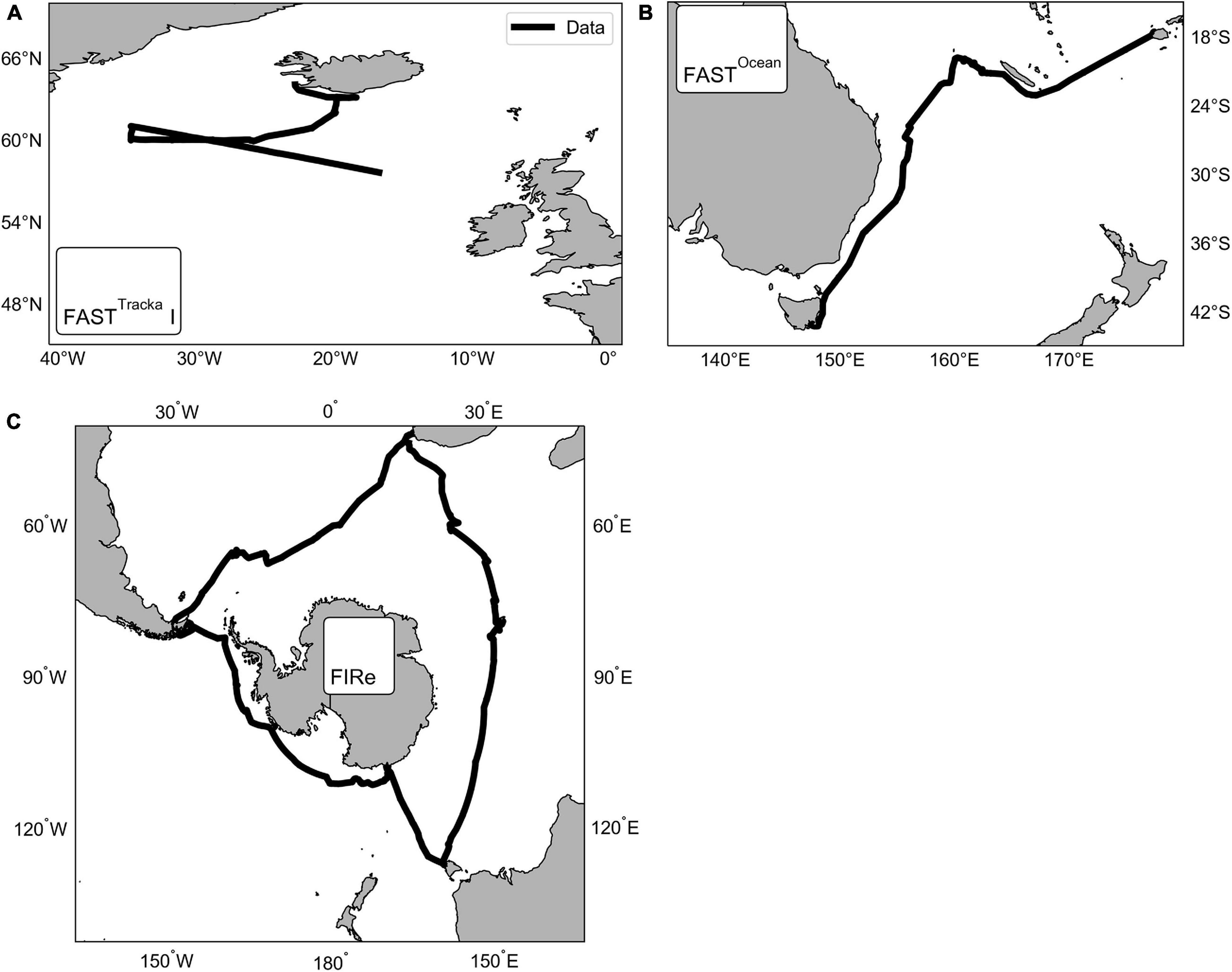
Figure 1. Maps showing the locations of the data collected using three different active chlorophyll fluorescence instruments, CTG (A) FAST^Tracka I (D350; North Atlantic) and (B) FAST^Ocean (IN2016_T01; South Pacific), and (C) Sea-Bird Scientific (previously Satlantic) FIRe (ACE; Southern Ocean).

(1) Chelsea Technologies Group (CTG) FAST^Tracka I (SN 05-4845-001): Data were obtained during the Irminger Basin Iron Study (IBIS) on a cruise of the RRS Discovery to the high latitude North Atlantic (D350) from 28 April 2010 to 10 May 2010 (Figure 1A). The CTG FAST^Tracka I was connected to the underway seawater supply to collect measurements in the dark chamber according to the data collection protocol outlined in Table 1. Data was converted from binary to a text file with bin2txt.exe program provided with the Laney V6 code Laney (2003, 2008).

TABLE 1

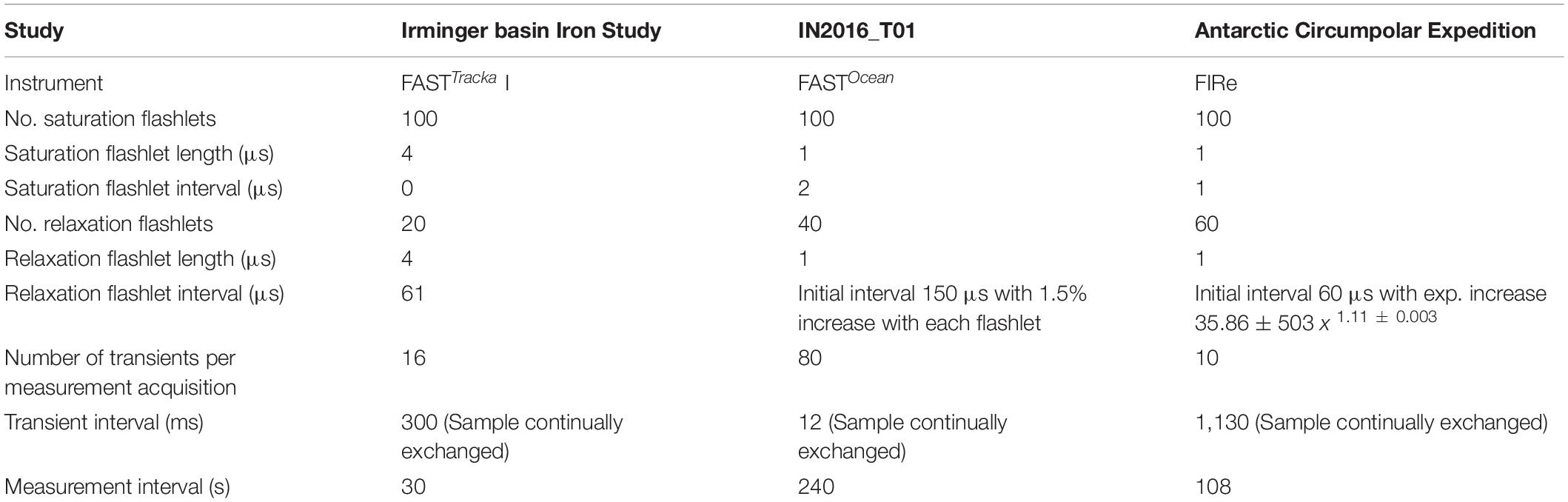
Table 1. Data collection protocols for the data presented as application of the Phytoplankton Photophysiology Utilities package.

(2) CTG FAST^Ocean (SN 12-8679-007): Data were obtained during the IN2016_T01 transit voyage of the RV Investigator between Lautoka, Fiji to Hobart, Australia from the 30 June 2016 to 14 July 2016 (Figure 1B). The CTG FAST^Ocean Instrument was connected to the underway seawater supply to collect measurements according to the data collection protocol in Table 1 using a combination of LEDs; blue (λ450 nm), blue+green (λ450+530 nm) and blue+orange (λ450+624 nm). Data was exported to a CSV file using the FastPro8 copy all function and pasted into an excel file. For the purposes of this analysis only data from the blue LED (λ450 nm) is reported.

(3) Satlantic (now Sea-Bird Scientific) FIRe (SN 030): Data were obtained during the Antarctic Circumnavigation Expedition (ACE) cruise of the RV Akademik Tryoshnikov around Antarctica from 20 December 2016 to 21 March 2017 (Figure 1C). The FIRe instrument was connected to the underway seawater supply to collect measurements according to the data collection protocol outlined in Table 1, the protocol consisted of only using the blue LED (λ455 nm) for the excitation flashlets. Original raw data files were exported with no conversions applied.

Particulate Absorption Data

Samples for particulate absorption were also collected and used to demonstrate spectral correction features of the Phytoplankton Photophysiology Utilities toolbox (see section “LED Spectral Correction”). Following the quantitative filter pad technique (Mitchell et al., 2002), 0.5–2 L of seawater were filtered onto 25 mm GF/F, snap frozen in liquid nitrogen and stored at −80°C for later analysis in a Shimadzu UV-2501 spectrophotometer. Optical density (OD) was measured using the internally mounted integrating sphere approach using an air baseline (Stramski et al., 2015) from 350 to 750 nm (1 nm resolution). Blank filter measurements were also collected. Phytoplankton particulate absorption coefficients were calculated with the Phytoplankton Photophysiology Utilities toolbox as explained in section “LED Spectral Correction.”

PPU Analytic Software and Optimization Algorithms

A custom analysis package, Phytoplankton Photophysiology Utilities (PPU) was developed to robustly analyse data from CTG FAST^Tracka I, CTG FAST^Ocean and Sea-Bird Scientific (previously Satlantic) FIRe instruments. More instruments are supported but will not be discussed further here. The package is available open source on the GitLab repository and free for use following the MIT license¹; the package can also be downloaded from the python package index (pip) with the command: pip install phyto_photo_utils. PPU was written in Python (V3.7;²) using robust optimization methods from the SciPy package (available at³). Additional dependencies include tqdm (available at⁴), numpy (Harris et al., 2020), pandas (available at⁵), matplotlib (available at⁶) and sklearn (available at⁷).

The default method in the PPU toolbox for least squares optimization uses a similar approach to Laney (2003), applying a trust region reflective algorithm (Coleman and Li, 1994, 1996) which reduces the potential of the estimated parameters becoming “trapped” in local minima or at the user defined boundaries. Further defined parameters for the loss function, tolerance limits and number of function evaluations before the termination allows the user to balance computational efficiency against computational time. The optimization routines fit the Kolber-Prasil-Falkowski biophysical model (KPF; Kolber et al., 1998) with a series of user defined functions and options for the saturation phase and the relaxation phase of the fluorescence induction curve (details below).

PPU Statistical Parameters for Data Quality Control

The PPU fitting routines return a suite of statistical parameters which assess the accuracy, bias and precision of the optimization routines and derived parameters, some of which, but not all are included in the output of manufacturer and custom written software for processing FRRf and FIRe data. Other software programs report the coefficient of determination (R²), χ² and reduced χ² as goodness of fit tests for the robustness of the non-linear model (Supplementary Table 1). However, we recognize that these metrics are not suitable tests for non-linear models (Andrae et al., 2010; Spiess and Neumeyer, 2010) or one-hit Poisson functions similar to the KPF model (Laney, 2003) and have chosen to exclude these metrics. The following statistical metrics were calculated for the model performance: root mean squared error (RMSE, Equation 1, Chai and Draxler, 2014) assessing accuracy between the fitted model and observed fluorescence yield; normalized RMSE where the mean squared error is divided by the mean fluorescence values (nRMSE, Equation 2); and normalized bias (modified from equation 3 of Seegers et al., 2018), calculated as Equation 3, indicating the systematic direction of the average difference or error between the model and observations. The precision of the fitted parameters is also assessed through fit errors, one standard deviation error for each derived parameter computed with an inverse jacobian covariance matrix normalized to the mean squared residuals. In cases of F_o and F_m the fit error values are returned as percentages so as to avoid any specific instrument bias on the parameter error interpretation. In each equation O_i and M_i are the nth flashlet of the observed and modeled fluorescence yield, respectively, and Ô is the mean observed fluorescence.

$$RMSE=\sqrt{\frac{{\mathrm{\Sigma }}_{i=1}^N{(M_i-O_i)}^2}{N}}(1)$$

$$nRMSE=\sqrt{\frac{{\mathrm{\Sigma }}_{i=1}^N{(M_i-O_i)}^2}{\underset{¯}{O}}}(2)$$

$$Bias=\sum _{i=1}^N\frac{M_i-O_i}{O_i}(3)$$

Functions of the Package

There are 17 functions available within the PPU toolbox (Figure 2), which are described in Supplementary Table S2. Detailed explanations of each function are given in the documentation online⁸ with examples in the GitLab repository demo Jupyter notebook⁹. Here we will demonstrate the application of the primary functions and assess their performance against select proprietary manufacturers software distributed with the instruments and custom-written open-source software from the chlorophyll-a fluorescence community.

FIGURE 2

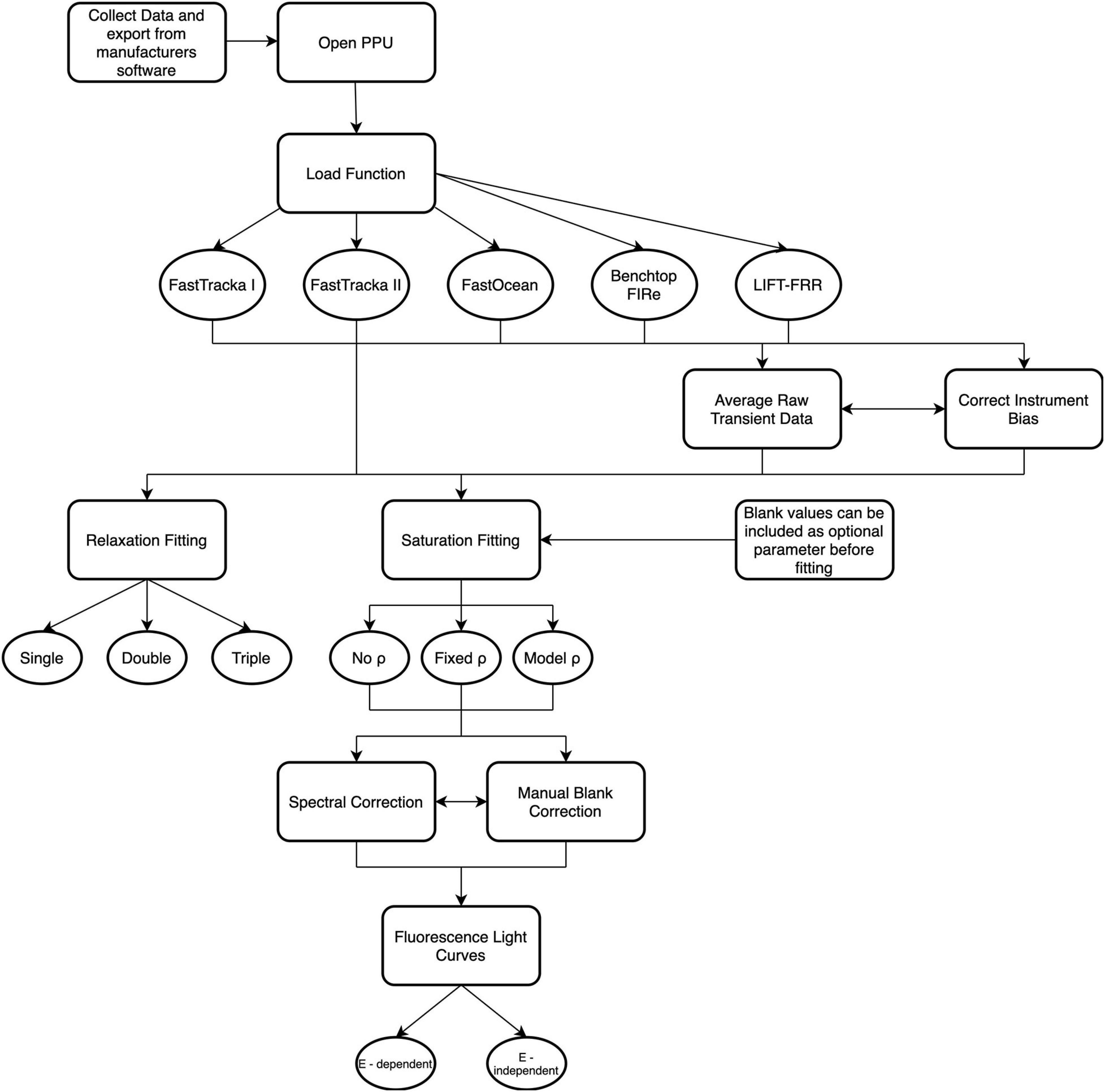
Figure 2. Schematic overview of the functions available within Phytoplankton Photophysiology Utilities. For further details on specific function descriptions see Supplementary Table 2.

Saturation Phase Fitting

The PPU toolbox offers three separate models to fit the saturation curve within the saturation.fit_saturation function, varying in the application of the connectivity coefficient ρ. Model 1, “no ρ” model (Equation 4; Equation 1 in Laney, 2010), assumes no connectivity between photosystems. Model 2, “ρ” model (Equation 5 and 6; Equation 1 from Kolber et al., 1998) assumes connectivity between photosystems and iteratively obtains a value for ρ. Model 3, “fixed ρ” model (Equations 5 and 6) also assumes connectivity between photosystems, but ρ is fixed with a user defined value (“fixed ρ” model). The “fixed ρ” model is commonly applied to datasets collected in low biomass ecosystems, where the chances of accurately estimating ρ are decreased (Suggett et al., 2001), see below for more details. The PPU toolkit includes fixed, and user set bounds to constrain the saturation parameter values. Fixed constraints are set for F_o as the intercept of a linear fit of the first eight fluorescence values ± 10%, for F_m as the intercept of the of the last 24 fluorescence values ± 10%, and ρ (where applicable) as 0 ≤ ρ ≤ 1. The functional absorption cross section σ_PSII ($\stackrel{°}{{\text{A}}^{\text{2}}}$ RCII^–1) bounds are user set (see Supplementary Table S3 for default bounds).

$$f_n=f_o+(f_m-f_o)\times (1-e^{(-\mathrm{\sigma }\times \mathrm{\Sigma }(pfd)}))(4)$$

$$f(t)=f_o+(f_m-f_o)\times \left[C(t)\frac{1-\mathrm{\rho }}{1-C(t)\mathrm{\rho }}\right](5)$$

$$\frac{dC(t)}{dt}=i(t){\mathrm{\sigma }}_{PSII}\frac{1-C(t)}{1-C(t)\mathrm{\rho }}-\frac{C(t)}{\mathrm{\tau }}(6)$$

Relaxation Phase Fitting

To parameterize the time constants of PSII reoxidation kinetics from the “relaxation” phase of a fluorescence induction curve, the PPU toolbox relaxation.fit_relaxation function can apply either a single exponential equation (Equation 7; Laney, 2003, 2010) or a triple exponential (Equation 8; Kolber et al., 1998) to parameterize the decay in fluorescence. The relaxation parameters are also constrained by bounds, with F_oRelax confined to the mean of the last three fluorescence values ± 10%, and F_mRelax between the mean of the first three fluorescence values ± 10%. In instances where the fluorescence decay of the first few flashlets of the relaxation phase is very rapid, a user defined number of flashlets from the end of the saturation phase of the fluorescence induction curve can be included to the mean calculations determining F_mRelax bounds to improve the estimate of F_mRelax. The relaxation time constants τ₁, τ₂, τ₃ and τ_PSII (thought to be equivalent to electron transport from Q_A- > Q_B- > PQ pool- > PS1), and corresponding amplitudes (α₁, α₂, α₃) are constrained by user defined values in μs and default values are presented in Supplementary Table S3.

$$f_n=f_{mRelax}-(f_{mRelax}-f_{oRelax})\times (1-e^{(-\mathrm{\Delta }t/\mathrm{\tau }PSII)})(7)$$

$$g(t-\mathrm{\nu })={\mathrm{\alpha }}_{1}e(-\mathrm{\Delta }t/{\mathrm{\tau }}_1)+{\mathrm{\alpha }}_{2}e(-\mathrm{\Delta }t/{\mathrm{\tau }}_2)+{\mathrm{\alpha }}_{3}e(-\mathrm{\Delta }t/{\mathrm{\tau }}_3)(8)$$

Instrument Bias and Correction Methods

Blank Correction

Fluorescent materials within the water column, such as colored dissolved organic material and other pigmented detrital material, although not capable of variable fluorescence, can still artificially inflate the background fluorescence yield resulting in an increase in F_o and F_m, and hence F_v/F_m (Cullen and Davis, 2003). The PPU toolbox can be used to calculate the blank fluorescence value from raw data files, under the assumption that background fluorescence has no variable yield. A blank correction can then be applied either during the fitting of the fluorescence induction curve or post-fitting by directly correcting F_o and F_m and F_v/F_m using the PPU calculated value or user set values. As the requirement for blank corrections has long been considered a best practice requirement (Cullen and Davis, 2003), the effects of blank correction will not be discussed further.

LED Spectral Correction

The spectra of the light emitting diodes (LED) supplying the excitation and actinic irradiances within the FRRf and FIRe instruments do not directly represent the natural available light field for phytoplankton photosynthesis in the water column or the action spectrum of photosynthesis for phytoplankton (Emerson and Lewis, 1942; Neori et al., 1986; Szabó et al., 2014). Failure to correct for these spectral differences can lead to over/underestimations of σ_PSII (Suggett et al., 2001; Szabó et al., 2014) and hence spectral correction is now considered best practice, where possible (Hughes et al., 2018). The PPU toolbox employs spectral correction using the most common approximation of the spectral dependency of light absorption by photosystem II (Suggett et al., 2004; Silsbe et al., 2015; Schuback et al., 2017), the phytoplankton specific particulate absorption spectrum [a_phy(λ)]. Other approximations include the use of a_phy(λ) corrected for photosynthetic vs non-photosynthetic pigments and the fluorescence excitation spectrum derived from passive or active spectral fluorescence measurements (Silsbe et al., 2015). PPU provides two functions to achieve this goal; calculating the phytoplankton specific particulate absorption coefficients from measurements of optical density and calculating spectral correction factor (SCF) for correction of σ_PSII and the actinic light (where used) such as in the CTG FAST^Act system used for fluorescence light curves.

Following the IOCCG best practice protocols for spectrophotometric measurements of particulate absorption using filter pads (IOCCG Protocol Series, 2018), the PPU function calculate_chl_specific absorption provides options to subtract blank filter measurements and calculate total particulate absorption from the optical density as per Equation 9 (Equation 5.3 and 5.4 in IOCCG Protocol Series, 2018) where OD_f is the blank corrected optical density of the sample filter (absorbance; with option to normalize to infrared wavelengths), V is the volume of sample filtered (m³), A is the effective (sample) area of the filter (m²) and β₁ and β₂ are the coefficients for the pathlength amplification accounting for scattering through the filter (see Stramski et al., 2015 for the method appropriate coefficients to apply).

$$a(\mathrm{\lambda })=ln(10){\mathrm{\beta }}_{1}O{D}_f{(\mathrm{\lambda })}^{{\mathrm{\beta }}_2}/(V/A)(9)$$

If users have depigmented absorbance measurements (i.e., optical density of non-algal particles after removal of pigments with an extraction solvent) then these measurements can be subtracted to yield phytoplankton specific particulate absorption a_phy(λ). Alternatively, the non-algal contribution to the total particulate absorption measurements can be algebraically calculated using an iterative best-fit approach of Bricaud and Stramski (1990) to determine the absorption by non-algal particles and hence a_phy(λ). If phycobiliprotein pigment concentrations or other accessory pigment concentrations such as chlorophyll-b or chlorophyll-c concentrations are high (or suspected) in the measured sample, the selection of the green wavelength absorption (at 580 nm) may not satisfy the criteria that absorption by pigments must be minimal at 580 nm so that the ratio with 692 nm is close to 1. The PPU offered solution is to find the green wavelength between 580 and 600 nm which best satisfies the requirements, although it is acknowledged that this is not a perfect solution. Finally, the calculated a_phy(λ) can be normalized to a user set chlorophyll-a concentration to yield the chlorophyll-specific phytoplankton absorption coefficients a*_phy(λ)(m² mg chla^–1).

The function calculate_instrument_led_correction calculates the spectral correction factor for correcting either σ_PSII or the actinic light as needed by the user. The function utilizes the phytoplankton particulate absorption coefficient spectra [a_phy(λ), can also be chlorophyll specific a*_phy(λ)] calculated as above or input by the user. For correcting σ_PSII as Equation 10, the instrument LED spectra [E_LED(λ) 400–700 nm] and background light E_background(λ, 400–700 nm) as either the instrument actinic light E_actinic(λ, 400–700 nm) or in-situ light field E_in–situ(λ, 400–700 nm) are required. For correcting the actinic light both E_actinic(λ,400–700 nm) and E_in–situ(λ,400–700 nm) are required (Equation 10). The E_LED(λ, 400−700nm) for the FIRe, FAST^Trackka and FAST^Ocean instruments and E_actinic(λ, 400–700 nm) for the FAST^Act system used in this study are provided in example files with the PPU package. As the measurement of in-situ light fields (400–700 nm) are not always common practice in field studies the PPU toolbox can calculate a representative in-situ light field (spectral distribution of irradiance 400–700 nm) using a modified approach of Stomp et al. (2007b, a) and Schuback et al. (2015). The in-situ light spectrum 400–700 nm at depth z is estimated as Equation 12 using a typical incident solar spectrum (400–700 nm from Stomp et al., 2007b,a) and the spectrally dependent light attenuation coefficient [k_d(λ)]. Following Morel et al. (2007), k_d(λ)(Equation 13a and 13b) is equal to attenuation by pure seawater (a_w(λ) from Pope and Fry (1997) and $\frac{1}{2}{b}_w(\mathrm{\lambda })$ from Morel (1974)) and attenuation by phytoplankton, non-algal particles and cultured dissolved organic material as k_bio calculated as a function of chlorophyll-a using the coefficient χ(λ) and exponent c(λ). The spectral correction factors for σ_PSII or the actinic background light are then calculated as Equations 10 and 11, respectively, where E_LED(λ), E_in–situ(λ), E_background(λ), E_actinic(λ) and a_phy(λ) have been normalized to the maximum value of their respective spectra:

$$SCF{\mathrm{\sigma }}_{PSII}=\frac{{\mathrm{\Sigma }}_{400}^{700}{a}_{phy}(\mathrm{\lambda })E_{background}(\mathrm{\lambda }){\mathrm{\Sigma }}_{400}^{700}{E}_{LED}(\mathrm{\lambda })}{{\mathrm{\Sigma }}_{400}^{700}{a}_{phy}(\mathrm{\lambda })E_{LED}(\mathrm{\lambda }){\mathrm{\Sigma }}_{400}^{700}{E}_{background}(\mathrm{\lambda })}(10)$$

$$SCFactinic=\frac{{\mathrm{\Sigma }}_{400}^{700}{a}_{phy}(\mathrm{\lambda })E_{actinic}(\mathrm{\lambda }){\mathrm{\Sigma }}_{400}^{700}{E}_{in-situ}(\mathrm{\lambda })}{{\mathrm{\Sigma }}_{400}^{700}{a}_{phy}(\mathrm{\lambda })E_{in-situ}(\mathrm{\lambda }){\mathrm{\Sigma }}_{400}^{700}{E}_{actinic}(\mathrm{\lambda })}(11)$$

$$E(z,\mathrm{\lambda })=E(z,\mathrm{\lambda })=E(0,\mathrm{\lambda })\times e^{(-k_d\times z)}(12)$$

$$k_d(\mathrm{\lambda })=k_w(\mathrm{\lambda })+k_{bio}(\mathrm{\lambda })(\mathrm{13a})$$

$$k_d(\mathrm{\lambda })=a_w(\mathrm{\lambda })+\frac{1}{2}{b}_w(\mathrm{\lambda })+(\mathrm{\chi }(\mathrm{\lambda })=ch{l}^{c(\mathrm{\lambda })})(\mathrm{13b})$$

Optimization in Low Biomass Systems

In low biomass waters the signal-to-noise ratio can significantly impact the accuracy of the optimization routine fitting fluorescence induction curves and the robustness of the fitted results (Suggett et al., 2005). This is of particular importance when operating the instruments in an underway mode and sampling across vast biogeochemical regimes with large dynamic ranges in biomass concentrations. To improve the signal-to-noise, convergence of the model fitting and accuracy of results, fluorescence transients can be merged or averaged before fitting using the tools.remove_outlier_from_time_average function. As there are large discrepancies in sampling protocols across the active chlorophyll-a fluorescence community, this function employs merging of fluorescence induction transients within a user set time window rather than achieving a set number of acquisitions per measurement average. An additional option is to exclude transients within the time window that exceed a user defined number of standard deviations of the mean.

FIRe Measurement Bias Correction

Benchtop FIRe instruments use a reference excitation profile measured with fluorescent dye in place of direct measures of the incident LED excitation intensity to normalize the fluorescence emission and generate the fluorescence yield (Satlantic LP, 2010). Manufacturers of the FIRe instrument, Satlantic (now Sea-Bird Scientific; note that the instrument is now discontinued) generally supplied two instrument-specific factory default reference excitation profiles for use with different gain settings. However, noticeable artifacts appear in FIRe fluorescence yield where there is a mismatch between the reference excitation profile and actual incident excitation irradiance. Artifacts in the saturation phase may include a large difference in between the fluorescence yield of the first and second flashlet (Supplementary Figure 1A) as the LEDs are warming up after being turned on, which in some extreme cases can be more than 100% greater than the average flashlet difference. As the excitation protocol transitions from the saturation to relaxation phase, a second significant mismatch occurs between the reference profile and actual incident LED irradiance. This results in a large difference between the last flashlet of the saturation phase and the first flashlet of the relaxation phase (Supplementary Figure 1A) possibly due to a time lag during the protocol switch, as well as a significant drop in fluorescence yield of the relaxation phase (far below F_o of the saturation phase) roughly equal to the difference between the last flashlet of the saturation phase and the first flashlet of the relaxation phase (Z. Kolber in pers. comm.). These biases have significant impact upon the fitted results which will be discussed later (see Section “Measurement Bias Correction”). In the release of custom software code FIReworx (Barnett, 2007) for processing FIRe data, Barnett (now Ciochetto) advocated strongly for individual users to collect their own repeated reference excitation profile measurements with fluorescent dye Rhodamine Blue to account for the mismatch during the transition from saturation to relaxation phases of the measurements and to drop the first flashlet (or first few flashlets) from the saturation fitting process. In the case that custom reference excitation profiles are not available or where custom profiles still do not correct the bias the PPU toolbox provides options to correct the bias. Within the saturation.fit_saturation function users can utilize options to ignore flashlets from the start of the saturation phase during fitting. In addition to improving estimates of F_mrelax via the relaxation.fit_relaxation function as detailed in section “Relaxation Phase Fitting,” users can employ tools.correct_fire_instrument_bias to correct the fluorescence yield of the relaxation phase by adding the difference between the first flashlet of the relaxation phase and a user set position in the relaxation fluorescence yield (e.g., second flashlet) to all flashlets in the relaxation phase (except the first flashlet; Supplementary Figure 1B).

Demonstration of PPU and Statistical Comparisons

Demonstration of PPU Functions

To demonstrate the sensitivity, reliability and advantages of the PPU toolbox for fitting single turnover fluorescence transients, data from the FIRe, FAST^Tracka I and FAST^Ocean were fit using the PPU toolbox and available manufacturers software or custom open-source code.

To demonstrate saturation phase fitting by the PPU toolbox, the “ρ” saturation model was selected within the saturation.fit_saturation function to process data from the FIRe, FAST^Tracka I and Fast^Ocean. FIRe and Fast^Ocean data processing from PPU were compared with manufacturer software, FIRePro (V1.3.2) and FastPro8 (V1.0.55, supplied with the benchtop FIRe and Fast^Ocean instruments, respectively). As the analytic software originally supplied with the FAST^Tracka I (FRS.EXE) is no longer supported by the manufacturer, data from this instrument was processed with the publicly available custom fluorescence yield analysis software, V6, developed for MATLAB by Laney (2003) and an iteration of the software provided (in pers. comm.) by C.M. Moore (presented in Moore et al. (2007)) which applies the same fitting routines but also reports fit errors. To demonstrate relaxation phase fitting by the PPU toolbox, FAST^Ocean data was processed with the relaxation.fit_relaxation function using both the triple exponential decay model to derive τ₁, τ₂ and τ₃, and single decay model to derive τ_PSII. Both models were applied in order to compare to FastPro8 (v1.0.55) as the software only returns a single decay value τ which is akin to τ₁. All data from the FIRe and FAST^Ocean were blank corrected prior to fitting. Blank measurements were not available for the FAST^Tracka I data. The upper and lower bounds for the various derived parameters were not changed from the preset in the Laney V6 code and modified Laney code (see Supplementary Table S4 for bounds and initial estimates) and could not be changed within proprietary software FastPro8 (v1.0.55) and FIRePro (V1.3.2). After fitting by PPU or other software/code, modest filtering was performed to remove data points where F_v/F_m was > 0.65 or F_v/F_m < 0, ρ < 0.001 or ρ > 1 and σ_PSII < 0 or σ_PSII > 2,000 and any of the returned τ parameters were equal to the set upper or lower limits.

Statistical Comparisons Between PPU and Other Software

Parameters derived from the PPU toolbox and various manufacturers and custom software were contrasted and assessed using linear least-squares regression, the mean absolute relative difference [Software MARD, Equation 14 (Gerbi et al., 2016)] and the Software Model Bias (Equation 15, Seegers et al., 2018) where M1_i and M2_i are the nth derived parameters from two different software/code fitting routines. Two variants of the least-squares optimization algorithm were also compared for performance, the trust region reflective and Levenberg-Marquardt algorithms using the Software MARD and Software Model Bias statistics. The Software MARD provides an assessment of the overall error (or difference) between the outputs from two different softwares, whereas the Software Model Bias provides a simple description of the direction of the error between the two software outputs.

$$SoftwareMARD={10}^{\frac{1}{N}{\sum }_{i=1}^N\left|\frac{lo{g}_{10}M{1}_i-lo{g}_{10}M{2}_i}{lo{g}_{10}M{2}_i}\right|}(14)$$

$$SoftwareModelBias={10}^{\left(\frac{{\sum }_{i=1}^{N}lo{g}_{10}(M{1}_i)-lo{g}_{10}(M{2}_i)}{N}\right)}(15)$$

Additional functions within the PPU toolbox are presented here to highlight best efforts to reduce uncertainties in processing single turnover fluorescence data. The derived value of the connectivity coefficient ρ can have a significant impact upon other retrieved parameters. To investigate the effect large uncertainties and hence the value of the connectivity coefficient ρ on F_v/F_m and σ_PSII, a series of sensitivity tests were performed where the connectivity coefficient was fixed at set values (0.1–0.9) using the saturation.fit_saturation function with “fixed ρ” model and the results were compared to the recommended value of ρ = 0.3 (Suggett et al., 2001). The correction of biases in the FIRe dataset and attempts to improve the signal to noise is demonstrated through application of the saturation.fit_saturation option to ignore the first flashlet and the tools.remove_outlier_from_time_average function, modifying the set time window from 3–30 min and excluding values ± 3 S.D of the mean within the time intervals, and fitting the fluorescence transients with the saturation.fit_saturation “ρ,” and the resulting change in RMSE and fit errors are reported. Finally spectral correction of σ_PSII is demonstrated on the same FIRe dataset using the _spectral_correction.calculate_chl_specific absorption and _spectral_correction.calculate_instrument_led_correction functions.

Results

Laney Code Versus Phytoplankton Photophysiology Utilities (FAST^Tracka I, North Atlantic, D350)

Retrieved parameters, F_v/F_m and σ_PSII from the PPU toolbox and Laney (2003) V6 code (referred to as LC from here, Figure 3) for the FAST^Tracka I dataset from the North Atlantic (D350) were highly linearly correlated (R = 0.99 and 0.96, respectively), with slopes close to 1 for F_v/F_m (0.94; Figure 3A) and σ_PSII (1.18; Figure 3B). The PPU code provides more statistical assessments than the V6 code, including the root mean squared error (RMSE), normalized RMSE, the bias of the fit as well as the fit errors for the retrieved parameters. The retrieved results had mean and median RMSE values of 0.006 and 0.004 for D350, with a mean bias of 0.05. Fit errors averaged 0.005 ± 0.004 (2.6% mean error) for F_o, 0.0007 ± 0.0004 (0.2% mean error) for F_m, 21.27 ± 13.00 (5.1% mean error) for σ_PSII and 0.13 ± 0.10 (33% mean error) for ρ. Average fit errors from the modified LC (MLC) were similar 0.006 ± 0.004 (3% error) for F_o, 0.001 ± 0.001 (0.4% error) for F_m, 19.9 ± 12 (4.4% error) for σ_PSII and 0.11 ± 0.06 (38% error) for ρ and the modified LC results were also highly linearly correlated with PPU results (Supplementary Figure 2). The F_v/F_m and σ_PSII Model Bias analyses demonstrate no distinctive biases (9% underestimation to 12% overestimations: Figures 4D,E) between PPU and LC, MLC processing codes. Compared to PPU, the LC processing code slightly overestimated F_v/F_m by 5% and σ_PSII by 12%. The Software Model MARD of 3–13 % for F_v/F_m and σ_PSII across all algorithms and codes (Figures 4A,B) reflects the scatter around the 1:1 lines observed in Figure 3. However, for ρ the Software Model Bias ranged from a 55% underestimation to a 40% overestimation in PPU vs other processing codes (Figure 4F) and the relative error (Software MARD) far exceeded 100 % (Figure 4C).

FIGURE 3

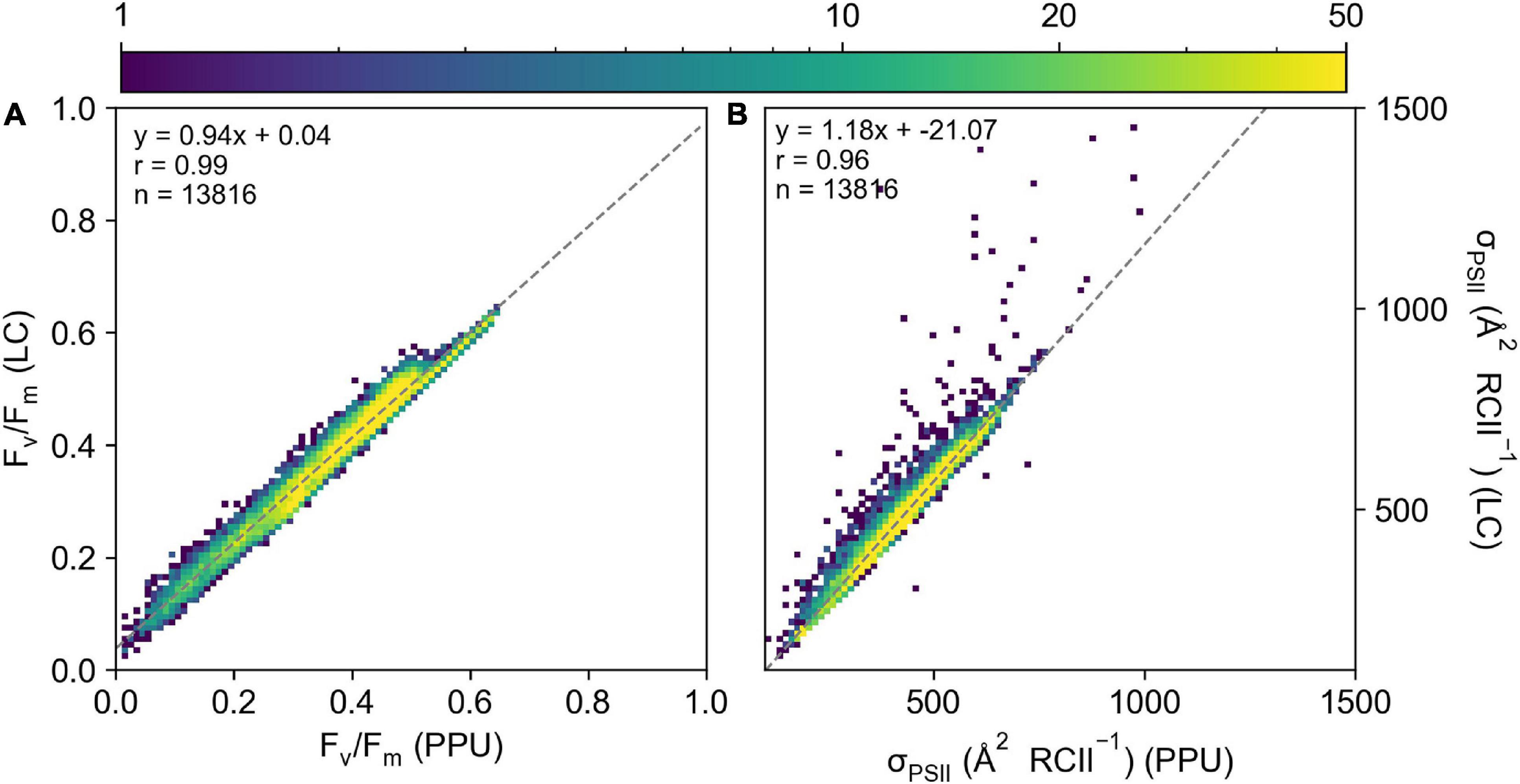
Figure 3. A 2D histogram of (A) F_v/F_m and (B) σ_PSII ($\stackrel{°}{{\text{A}}^{\text{2}}}$ RCII^–1) from the LaneyV6 code (y-axis) versus PPU (x-axis) from the D350 FAST^Tracka I dataset from the North Atlantic. The “ρ” model was used in both fitting routines.

FIGURE 4

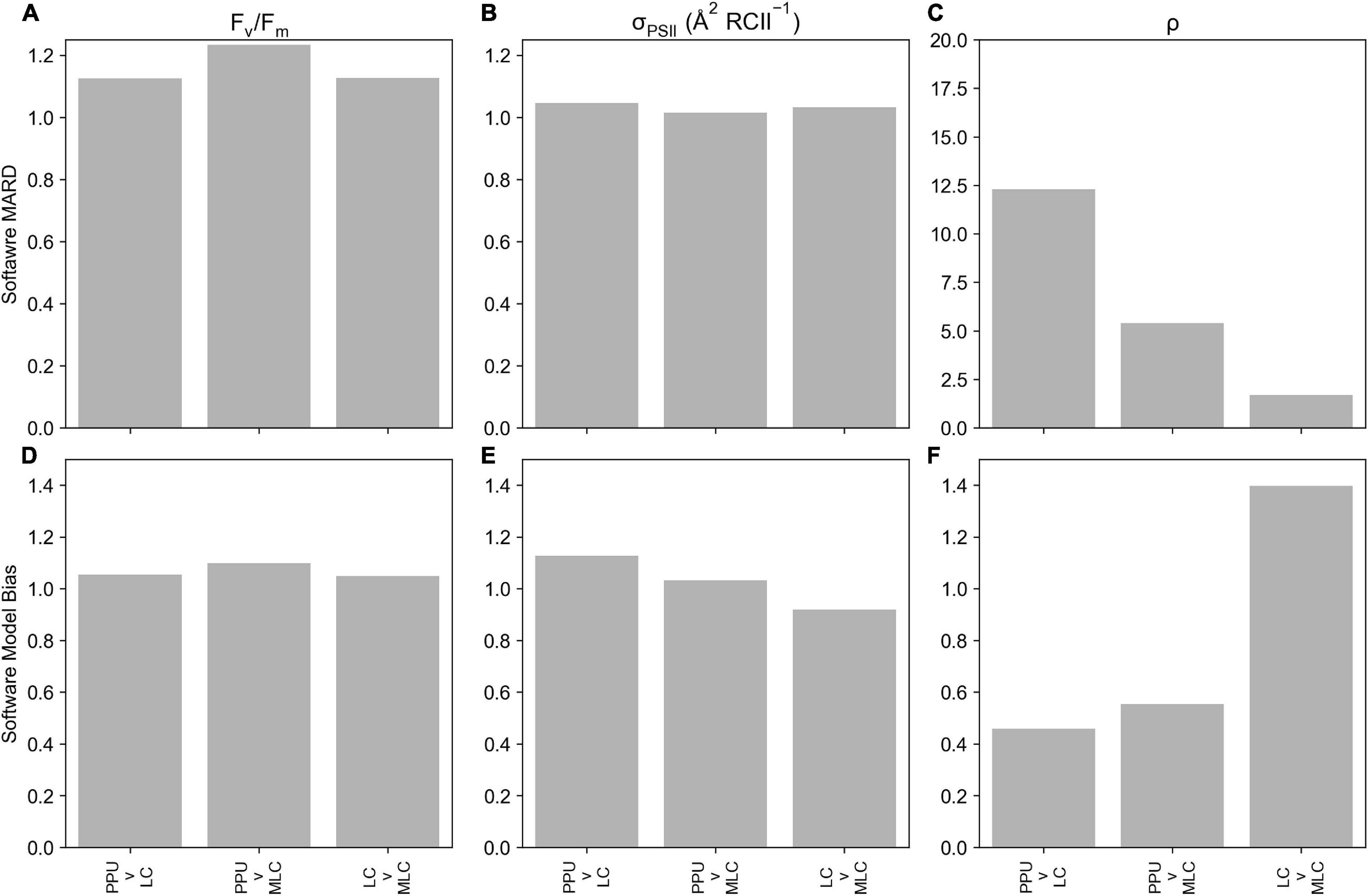
Figure 4. Statistical metrics comparing parameters derived from PPU, Laney V6 Code (LC) and modified Laney V6 Code (MLC) processing of the D350 (FAST^Tracka I) dataset from the North Atlantic. This includes the Software MARD (a-c) and Software Model Bias (d-f) for F_v/F_m (A,D), σ_PSII (B,E) and ρ (C,F). Please note the different scale in panel c.

Overall PPU produced similar estimates of F_v/F_m and σ_PSII from the FASTTracka I (North Atlantic, D350) dataset as compared to the Laney Code. There are substantial differences in the estimates of ρ, which is explored further in the discussion.

FastPro 8 Software (V1.0.55) Versus Phytoplankton Photophysiology Utilities (Fast^Ocean, South Pacific, IN2016_T01)

The mean and median RMSE of FAST^Ocean saturation fluorescence transients from the South Pacific (IN2016_T01) fit with PPU were 0.0064 and 0.0058, respectively. Mean fit errors were reasonable for F_o (0.004 ± 0.002, 2.3 % mean error) and F_m (0.001 ± 0.003, 0.75 % mean error), σ_PSII (48.67 ± 52.46, 13% mean error). However, the fit errors for ρ were considerably higher (0.25 ± 0.15, 269 % mean error).

Generally, there is good agreement between derived parameters from FastPro8 and PPU (n = 4,244 σ_PSII, n = 4,250 for F_v/F_m) with correlation coefficients for least-squares linear regression of 0.98 and 0.90 for F_v/F_m (Figure 5A) and σ_PSII (Figure 5B) respectively, with slopes ranging from 0.81 to 0.96. Derived estimates of ρ were poorly correlated between FastPro8 and PPU (Figure 5C; n = 3473). The lower sample size for ρ is due to the FastPro8 not always returning a value. The Software MARD between F_v/F_m from PPU and FastPro8 was 9% with FastPro8 typically 3% higher (Figure 5D). For σ_PSII the Software MARD was 4% and FastPro8 produced values 11% lower (Figure 5D). There was a strong positive model bias toward higher ρ values reported by PPU (7.01; Figure 5E), i.e., FastPro8 values were 50% lower. Moreover, the values of ρ ranged from 0.002 to 0.371 within the FastPro8 results, whereas they ranged from 0 to 0.99 within PPU. As a result, the Software MARD between PPU and FastPro8 was > 100%.

FIGURE 5

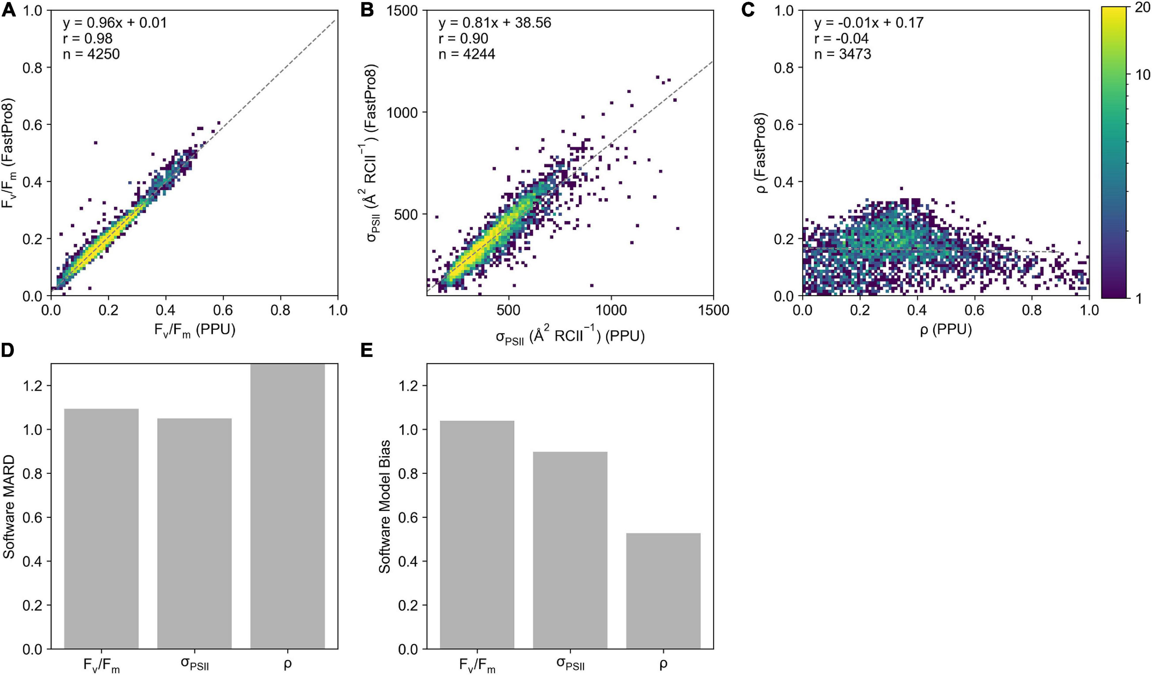
Figure 5. A 2D histogram of F_v/F_m (A), σ_PSII ($\stackrel{°}{{\text{A}}^{\text{2}}}$ RCII^–1) (B), and ρ (C) from the FastPro8 software (y-axis) versus PPU (x-axis) processing of FAST^Ocean data from the South Pacific (IN2016_T01). Bar charts of (D) software MARD (%) and (E) software model bias calculated between FastPro8 and PPU. Note that the Software MARD for ρ in panel (D) is out of the axis range.

The fitting of the relaxation phase to derive the decay time constant τ (μs) was performed using both the single and triple decay method as the FastPro8 software only returns a single decay τ value for the initial part of the relaxation phase (akin to τ₁). Both the single decay τ_PSII (Figure 6A) and triple decay τ₁ (Figure 6B) values from PPU were compared to the FastPro8 τ₁. The decay parameters derived from PPU were poorly correlated (Figures 6C,D), although FastPro8 consistently produced larger values of τ₁ compared to the triple decay τ₁ values from PPU. The triple decay τ₁ values are also significantly different from the FastPro8 τ₁ values (Wilcoxon Signed-Rank test, p > 0.05). The single τ_PSII values from PPU spanned a wider range of 110–49,046 μs than the FastPro8 τ₁ values of 157–1,840 μs (Figure 6A). It should be noted that the sample size of the FastPro8 results is much lower (n = 133) than the PPU (n = 2,171) output, suggestive of an issue with the manufacturer software to derive τ₁.

FIGURE 6

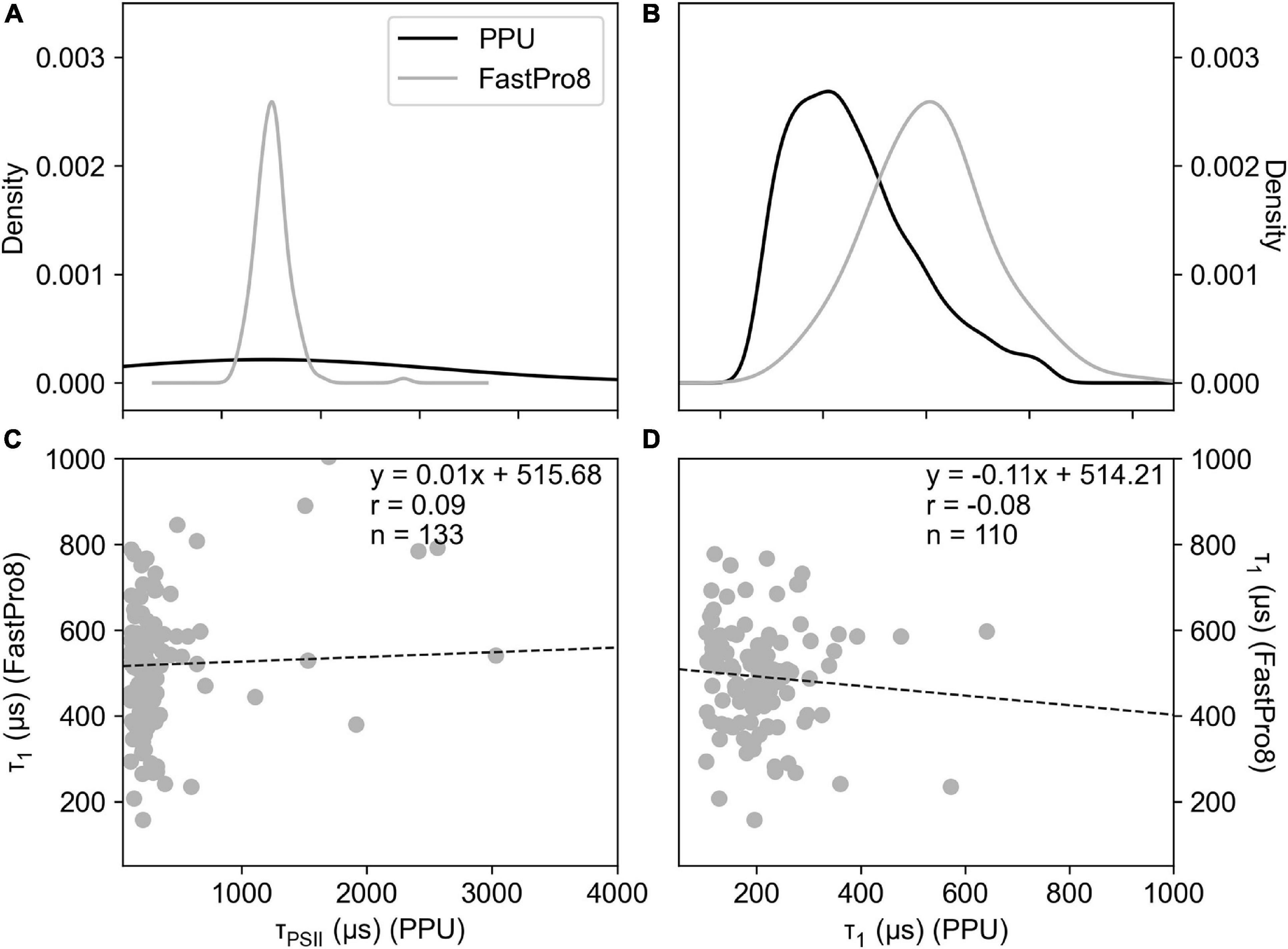
Figure 6. Density histograms of τ (μs) from the fitted results of FastPro8 τ₁ and PPU using the single decay τ_PSII (A,C) and triple decay (τ₁) (B,D) fitting routines using FAST^Ocean data from the South Pacific (IN2016_T01). Correlation plots of FastPro8 τ₁ (Y-axis) and PPU (X-axes) using the single decay (C) and triple decay (D) fitting routine.

The PPU processing of FastOcean data from the South Pacific (IN2016_T01) also produced similar values of Fv/Fm and σPSII as compared to the FastPro8 software, but estimates of ρ were again very different, likely due to ρ apparently being constrained to an upper limit of 0.4 in the FastPro8 software. Estimates of the decay time constant τ also varied substantially between PPU and FastPro8, due to the differences in the fitting equation, and is discussed further in the discussion.

Uncertainties in the Estimation of the Connectivity Coefficient (Fast^Ocean, South Pacific, IN2016_T01)

The value of the connectivity coefficient, ρ, in FAST^Ocean data from the South Pacific (IN2016_T01), demonstrated a significant impact on the value of other retrieved parameters from the saturation phase of fluorescence transients, specifically F_v/F_m (Figures 7A,C,E) and σ_PSII (Figures 7B,D,F). As compared to results when ρ = 0.3, percentage differences reached up to ∼55% for F_v/F_m and up to ∼35% for σ_PSII when the value of ρ increased. This resulted in a Software MARD that ranged from 4 to 56% for F_v/F_m (Figure 7C) and 1 to 6 % for σ_PSII (Figure 7D). Software Model Bias for σ_PSII was ∼1 (Figure 7E) but for F_v/F_m it decreased with increasing ρ to a minimum value of 0.72 (Figure 7F), representing a 28% underestimation relative to ρ = 0.3. Note that here, the “software” compared is PPU where ρ is fixed at values 0.1–0.9 as compared to PPU where ρ = 0.3. Uncertainties related to the estimation of ρ are explored further in the discussion.

FIGURE 7

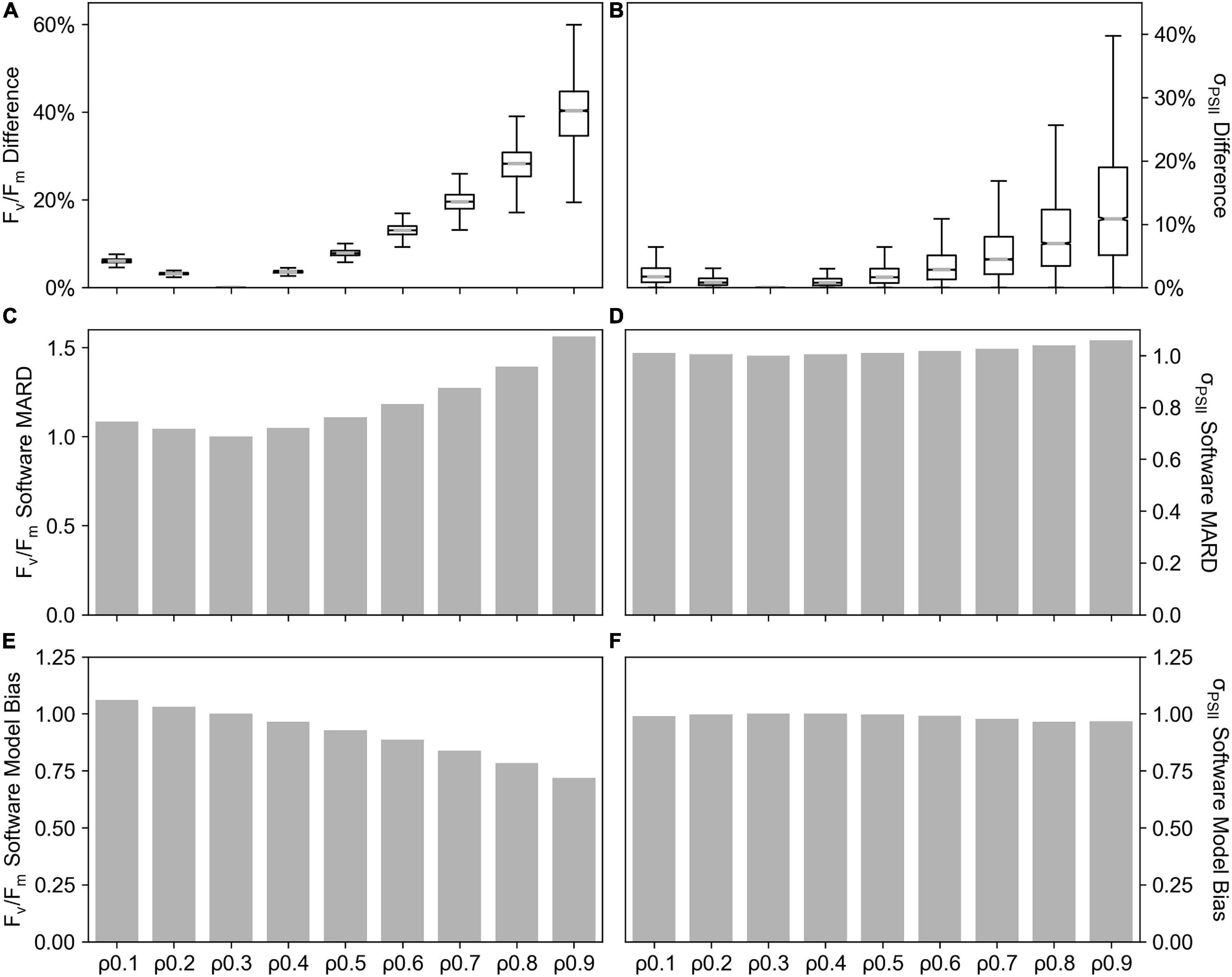
Figure 7. Connectivity coefficient (ρ) sensitivity tests performed on the Fast^Ocean data from the South Pacific (IN2016_T01). The percentage difference in F_v/F_m (A) an σ_PSII (B), Software MARD of F_v/F_m (C), Software MARD of σ_PSII (D), Software Model Bias in F_v/F_m (E) and Software Model Bias in σ_PSII (F) from ρ fixed at values 0.1–0.9 as compared to ρ = 0.3. Note that here, the “software” compared is PPU where ρ is fixed at values 0.10.9 as compared to PPU where ρ = 0.3.

FIRe Optimized Results Comparison (FIRe; Southern Ocean; ACE)

FIRePro Versus Phytoplankton Photophysiology Utilities

Derived parameters F_v/F_m and σ_PSII from the FIRe dataset from the Southern Ocean (ACE) processed by PPU do not agree well with the results from the FIRePro software (Figure 8). Linear correlations between the PPU and FIRePro derived parameters were poor at 0.12 and 0.28 for F_v/F_m (Figure 8A) and σ_PSII (Figure 8B) respectively. Note that no further optimization for signal-to-noise or instrument bias have been applied via either PPU or FIRePro. The results show that both retrieved parameters are much higher from the FIRePro software versus PPU, with many of the F_v/F_m results from FIRePro being above the theoretical maximum of 0.65 for single turnover protocols (Kolber and Falkowski, 1993). Fit errors reported in the PPU processed data were extraordinarily high at 37,805 ± 366,998 for F_o, 259 ± 9,970 for F_m, 17,241 ± 96,285 for σ_PSII and 137 ± 695 for ρ. Overall estimates of F_v/F_m and σ_PSII did not agree well between PPU and FIRePro.

FIGURE 8

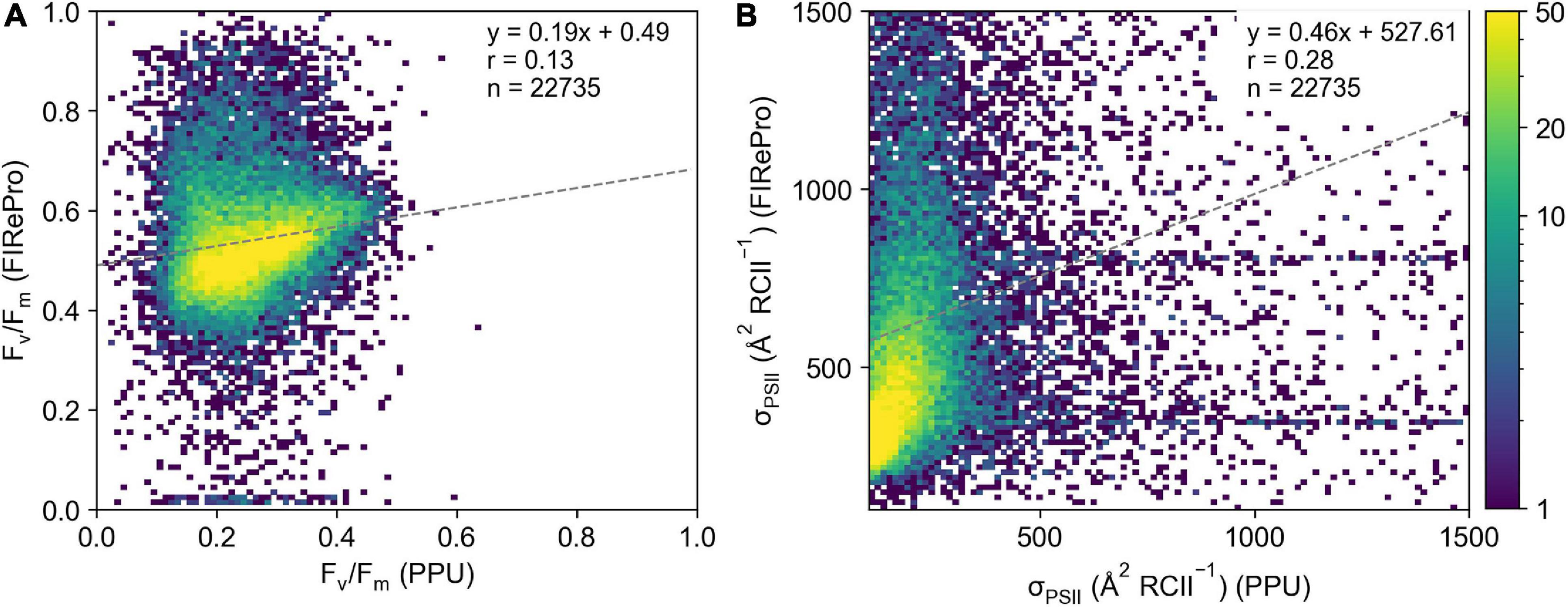
Figure 8. Comparison of (A) F_v/F_m and (B) σ_PSII derived from the FIRePro software (y-axis) and PPU (x-axis). Data is from the Southern Ocean (FIRe, ACE).

Measurement Bias Correction

The PPU option to correct a bias in the fluorescence transients of the FIRe dataset from the Southern Ocean (ACE) was applied, removing the first flashlet from the saturation fitting (see Supplementary Figure 1). The measurement bias correction decreased the median RMSE from 24 to 19 for the saturation phase fits (Figure 9A). This correction resulted in a shift in F_v/F_m values (Figure 9B), decreasing the mean values from 0.25 ± 0.08 to 0.21 ± 0.07 (∼16%), whilst also decreasing the mean σ_PSII values (Figure 9C) from 272.9 ± 235.8 to 219.8 ± 180.9 (∼19%). Moreover, there was a decrease in the fit errors, with a 72% decrease in σ_PSII error, an 84% decrease in F_o error and a 28% decrease in F_m error.

FIGURE 9

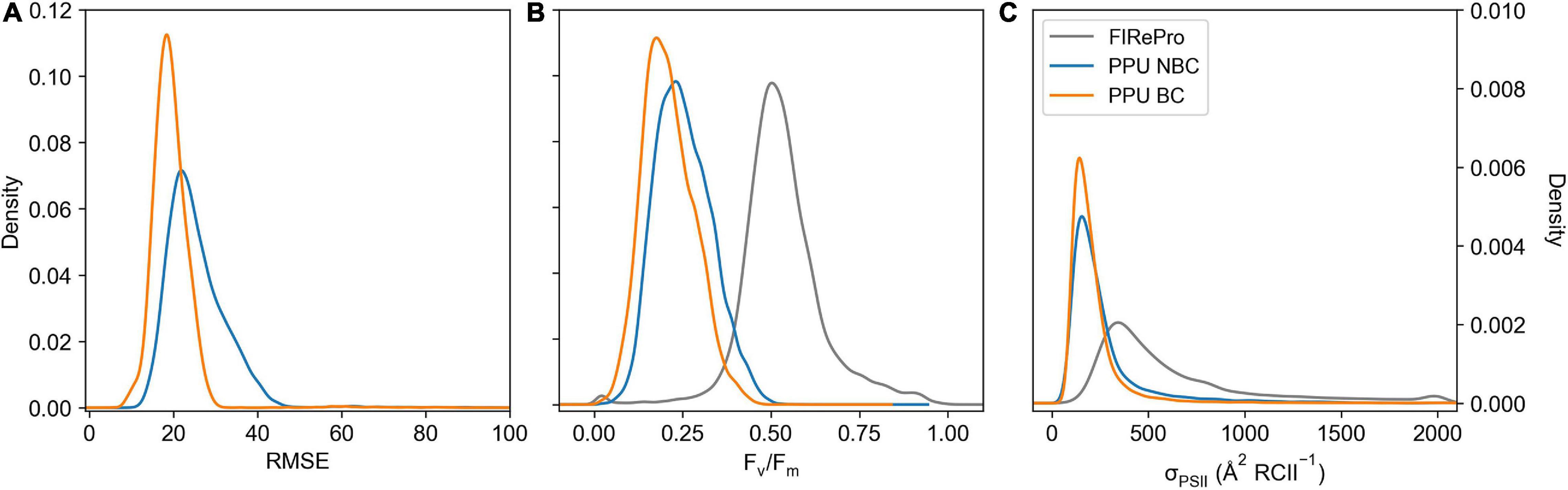
Figure 9. Kernel Density Estimation of FIRe saturation bias corrected (PPU BC) and uncorrected (PPU NBC) including RMSE (A), F_v/F_m (B), and σ_PSII ($\stackrel{°}{{\text{A}}^{\text{2}}}$ RCII^–1) (C), calculated using the calculate ρ saturation model. The F_v/F_m and σ_PSII results from FIRePro are also included in panels b and c. Data is from the Southern Ocean (FIRe, ACE).

Pre-optimization Transient Averaging

There was a change in the density distribution of the RMSE of fitted transients’ values as a result of increasing the time window over which the raw transient data is averaged or merged (Figure 10A), which resulted in a decrease in both the mean and median RMSE values (Figure 10B) and a decrease in the interquartile range (IQR; Figure 10B). For example, an increase in the time average to 10 min decreased the IQR by 133% decrease, which also led to a 53% reduction in the mean and median RMSE values. This shift in the relative robustness of the fit estimated from the RMSE values comes at a cost of the sampling resolution though, an 81% decrease in the number of measurements. The result of this is that a post-processing average will result in F_v/F_m values that are 6% lower than pre-processed averages (Supplementary Figure 3A) and σ_PSII values that are 16% lower (Supplementary Figure 3B). A threshold was identified however, at 21 min, after which wider time windows result in increasing RMSE and IQR values.

FIGURE 10

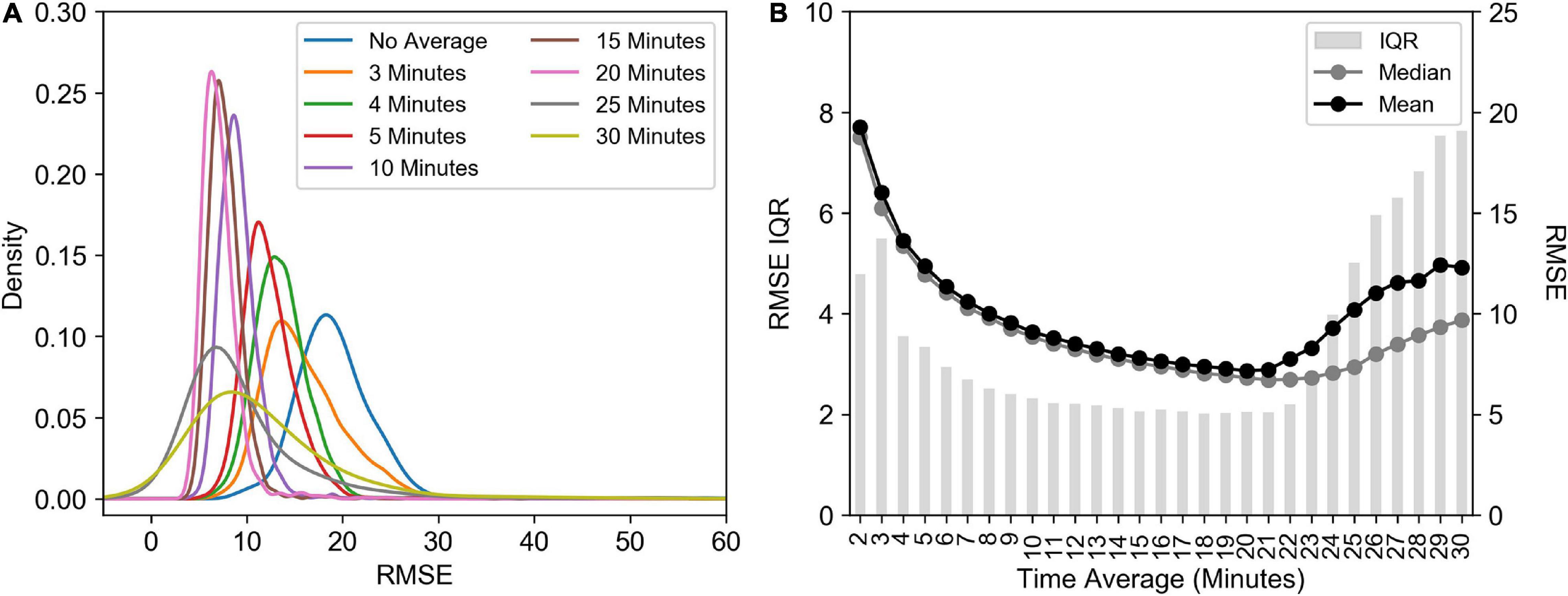
Figure 10. (A) Kernel Density Estimation of RMSE values calculated using different time window averaging using the calculate ρ saturation model. (B) The interquartile range (IQR), median and mean RMSE from the different time windows. All data presented here has been corrected for the FIRe instrument saturation bias, i.e., skipping the first flashlet. Data is from the Southern Ocean (FIRe, ACE).

Spectral Correction

The spectral correction factor (SCF) from the ACE voyage (Southern Ocean; FIRe) was calculated for 197 stations (Figure 11A), averaging 0.60 ± 0.04 (range = 0.46–0.77). To determine its effect upon a σ_PSII, an average of a ± 20-min time window was created for each station time point, this average σ_PSII,455 was then multiplied by the SCF to create σ_{PSII, in–situ} (Figure 11B). Across the time series there was an average difference between σ_{PSII, 455} and σ_{PSII, in–situ} of Δ 90.83 ± 65.55 ($\stackrel{°}{{\text{A}}^{\text{2}}}$ RCII^–1) (Δ range = 32.54–464.92; Figure 11C).

FIGURE 11

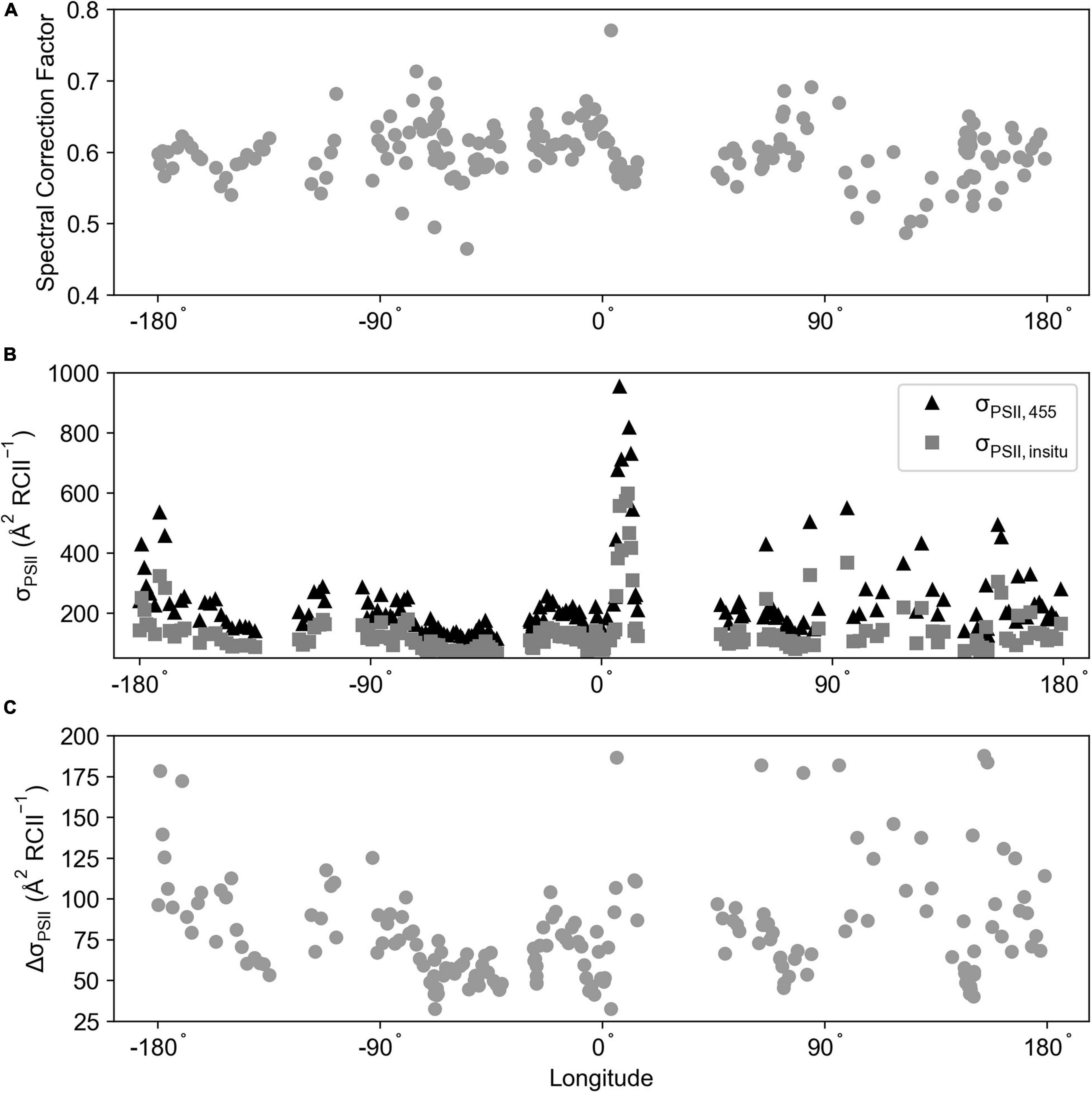
Figure 11. (A) The spectral correction factor calculated for the ACE voyage (Southern Ocean; FIRe) using Equation 9. (B) σ_{PSII, 455} and σ_{PSII, in–situ} ($\stackrel{°}{{\text{A}}^{\text{2}}}$ RCII^–1) averaged over a 20 ± time window of the absorption sample collection time. (C) The difference between σ_{PSII, 455} and σ_{PSII, in–situ} ($\stackrel{°}{{\text{A}}^{\text{2}}}$ RCII^–1). The σ_PSII values were calculated from bias corrected FIRe data.

Discussion

The aquatic single-turnover chlorophyll-a fluorescence user community has evolved considerably over the last two decades thanks to the growing commercial availability of user-friendly Fast Repetition Rate (FRRf) and Fluorescence Induction and Relaxation (FIRe) fluorometers. Whilst an array of proprietary software and open-source processing codes have served the FRRf/FIRe user community well for deriving photosynthetic parameters from fluorescence transients, the goal of global databases of high-quality single turnover fluorescence data (Lawrenz et al., 2013; Hughes et al., 2018) is not quite achievable with existing data processing tools. In particular no one software program in the current suite available provides adequate statistical metrics for quality control of data, allows for flexible application of the Kolber-Prasil-Falkowski (KPF) model, provides capacity for high-throughput processing (i.e., from continuously recorded datasets) and/or processes data from multiple models/brands of single turnover fluorometers. We have created PhotoPhytoUtils (PPU) to fill these critical gaps in single turnover fluorescence data processing and quality control in a bid to assist the chlorophyll-a fluorescence community to achieve its goals and progress our understanding of the natural variability of aquatic photosynthesis.

PhytoPhotoUtils (PPU) produced similar estimates of saturation phase photosynthetic parameters as compared to the FastPro8 software and open-source code V6 from Laney (2003) and modified version from Moore (presented in Moore et al. (2007)) used to process the FAST^Ocean and FAST^Tracka I data, respectively. The greatest difference was in the estimation of the connectivity parameter ρ which unlike PPU, was not constrained in the V6 and modified V6 code (See Supplementary Table 4) and the upper and lower bounds set for the algorithm solution are very likely to impact the final value of ρ. The difficulties in deriving accurate estimates of ρ have been well documented elsewhere (Suggett et al., 2001, 2004; Bruyant et al., 2005; Babin, 2008), especially in waters with low chlorophyll biomass. The ranges of chlorophyll concentrations in the surface during each campaign presented in this study were 0.5–5 μg/L in the Irminger Basin (Ryan-Keogh et al., 2013), <0.1–0.3 μg/L in the South-West pacific and East Australian Current (data not published) and 0.01–3.7 μg/L in the Southern Ocean (Antoine et al., 2019). Little is known by the authors about the fitting processes and bounds set for parameters within the FIRePro software which produced very different final parameters from FIRe data as compared to PPU output. The software and the desktop FIRe are no longer supported by the current owner company (Sea-Bird Scientific). The fit errors reported by PPU clearly demonstrate that without quality control, or correction beyond removing the blank influence, that the errors for all derived parameters are concerningly high and so it is not surprising that derived parameters from PPU and FIRePRO are poorly correlated. The decay time constants τ₁, and τ_PSII reported by PPU and FastPro8 were also poorly correlated, however, it is acknowledged that the fitting bounds set for these parameters, which are unknown for FastPro8, may strongly influence the final reported values complicating any comparison.

Allowing for the flexible application of the KPF model and modeling of the decay phase of single turnover fluorescence transients is important so that derived parameters can more accurately be compared to other processed datasets, and also to understand the natural variability of and uncertainties in the connectivity parameter ρ and the decay kinetics (τ). Open-source processing codes V6 (Laney, 2003), modified V6 (Moore et al., 2007) and fireworx (Barnett, 2007) provide these options for fitting FAST^Tracka (V6 and modified V6) and FIRe (fireworx) data. Our analysis of the uncertainties in the derived value of ρ and subsequent impact of the value of F_v/F_m and σ_PSII supports results from previous studies such as Babin (2008) that showed varying ρ between 0 and 0.6 can lead to variations in F_v/F_m of ∼20%. As compared to parameters derived when ρ was fixed at 0.3, the value of F_v/F_m varied up to 55 % and σ_PSII up to 35% when ρ varied between 0.1 and 0.9. As suggested by Suggett et al. (2001, 2004) applying the KPF model to saturation phase transient fits with ρ at a fixed value of 0.3 or constrained between 0.1 and 0.4 reduces the impact on F_v/F_m and σ_PSII. The value of τ, the time constant of PSII reoxidation, in nature is poorly understood. A quick Web of Science and Google Scholar literature search found 171 papers using single-turnover fluorometry to study photosynthetic parameters of phytoplankton between 1998 and 2019 and only 40 papers reported values of τ, with variations in the use of single exponential model and triple exponential models to parameterize the decay in fluorescence and the actual time constant reported (i.e., τ₁, τ₂, τ₃, and τ_PSII). The upper and lower limits set for τ₁, τ₂, τ₃, τ_PSII in PPU (See Supplementary Table S3) were constrained using these few examples. Based on the dataset collected from the South-west Pacific Ocean and East Australian current (FAST^Ocean dataset), the value of τ_PSII fell comfortably within the prescribed bounds of 100 μs to 50 ms (<5% of returned values were equal to the upper or lower bounds). It would appear though that τ₂ is much more rapid (64% of returned values were the lower limit of 800 μs) and τ₃ much longer (70% of returned values were the upper limit of 50 ms) than previously reported. The PPU package will provide the opportunity for the community to explore this variability in the time constants for the reoxidation PSII across a wide range of instruments and hence datasets.

Phytoplankton Photophysiology Utilities has incorporated a number of functions to improve the accuracy of single-turnover fluorescence transient fitting and to reduce biases and uncertainties resulting from background non-variable fluorescence (“blanks”), instrument specific characteristics and high noise in data from low chlorophyll biomass systems. Although not always employed, the correction for non-variable fluorescence from background dissolved fluorescent material (“blanks”) and spectral correction of σ_PSII are generally encouraged as standard practice (Cullen and Davis, 2003; Suggett et al., 2004), and so not discussed further here. Other open-source processing codes have drawn attention to the impact of various instrument specific artifacts in driving uncertainties in photosynthetic parameters and have provided relevant corrections (Laney, 2003, 2008; Barnett, 2007). As we have demonstrated here, failure to correct for the mismatch in the reference excitation profile within the desktop FIRe instrument will result in inflated F_v/F_m and σ_PSII values and high uncertainty in the estimates. When collecting observations in low-chlorophyll biomass ecosystems, protocols to maximize signal-to-noise such as repeated measurements or the averaging/merging of fluorescence transients before fitting must be employed. It has been suggested that uncertainties in derived parameters when signal-to-noise is low (or the absorption cross section is small) could be reduced through averaging of derived parameters after fitting (Suggett et al., 2005; Oxborough, 2013). However, using the desktop FIRe dataset as an example (See Supplementary Figure 3) there is a significant reduction in both the estimated values of σ_PSII and uncertainty of the estimates when transients within a 10-minute window are merged before fitting versus the averaging of the derived parameters after fitting. It must be recognized though that even after applying the various corrections to the fitting of single-turnover fluorescence transients that are available in PPU, considerable uncertainty still remains in the estimate of photosynthetic parameters, which is largely ignored by the single-turnover fluorescence community often because such information is not readily available. The mean fit errors of saturation phase parameters F_o, F_m, and σ_PSII derived from PPU ranged from reasonable values of 1–33% in the FAST^Tracka I and FAST^Ocean datasets to 31–1,050% percent in the FIRe dataset after bias correction and 9–217% percent after bias correction and transient merging within a 10-min interval. With the additional statistical metrics such as fit errors of the derived parameters and root mean square error of the fitting process, users of PPU can rapidly identify and remove data points with high uncertainty, significantly improving the quality of the processed dataset. When selecting a time window with which to average the user must remain aware of the different light histories that phytoplankton will be experiencing, i.e., day and night, and the length of time within a sampling system.

Phytoplankton Photophysiology Utilities is an open-source interface between python and active single-turnover chlorophyll-a fluorescence data that provides automated and standardized data processing for the chlorophyll-a fluorescence community. The PPU package has been developed with the intention that it evolves with community needs and knowledge that will improve the quality and usefulness of chlorophyll-a fluorescence data. As an open-source package, it is easily adaptable to incorporate recently published and future solutions and corrections, for example the “baseline” correction (Boatman et al., 2019). Planned future updates to the package will include support for the loading and processing of data from other fluorometers e.g., Satlantic in-situ FIRe, Satlantic miniFIRe, PSI Fluorometer and CTG LabSTAF, and the export of processed parameters to climate forecasting compliant netCDF format. Some additional functions currently exist in the package which were not featured here, including the fitting of photosynthesis vs irradiance models to fluorescence light curve data. As addressed above, the natural variability in reoxidation kinetics of the PSII-PSI electron chain is not well explored and consultation with the chlorophyll-a fluorescence community will be needed to improve the PPU relaxation kinetics functions and constrain the uncertainties in τ parameters. The PPU package provides increased capacity for users to take greater responsibility for the quality of their single-turnover fluorescence data and achieve community goals of building global databases of high-quality single turnover fluorescence data.

Data Availability Statement

The original contributions presented in the study are included in the article/Supplementary Materials, further inquiries can be directed to the corresponding author.

Author Contributions

TR-K and CR conceptualized the idea, wrote the python code, tested the code, collected the data for ACE, and wrote and edited the manuscript. TR-K collected the data for D350. CR collected the data for INV2016_T01 transit voyage. Both authors contributed to the article and approved the submitted version.

Conflict of Interest

The authors declare that the research was conducted in the absence of any commercial or financial relationships that could be construed as a potential conflict of interest.

Funding

This work was undertaken and supported through CSIR’s Southern Ocean Carbon and Climate Observatory (SOCCO) programme (http://socco.org.za). This work was supported by CSIR’s Parliamentary Grant (SNA2011112600001) and supported by the Australian Government through the Australian Research Council’s Discovery Projects funding scheme (project DP DP160103387).

Acknowledgments

We would like to thank the captains and crews of the RRS Discovery, the RV Investigator and the RV Akademik Tryoshnikov for their professional support throughout the cruises. We would also like to thank the SCOR working group 156 for their feedback on package utilization. The Antarctic Circumnavigation Expedition was made possible by funding from the Swiss Polar Institute and Ferring Pharmaceuticals. Finally, we wish to thank the CSIRO Marine National Facility (MNF) for its support in the form of sea time on RV Investigator, support personnel, scientific equipment and data management. All data and samples acquired on the voyage are made publicly available in accordance with MNF Policy.

Supplementary Material

The Supplementary Material for this article can be found online at: https://www.frontiersin.org/articles/10.3389/fmars.2021.525414/full#supplementary-material

Footnotes

1. ^ https://gitlab.com/tjryankeogh/phytophotoutils
2. ^ www.python.org
3. ^ www.scipy.org
4. ^ www.tqdm.github.io/
5. ^ www.pandas.pydata.org/
6. ^ www.matplotlib.org/
7. ^ www.scikit-learn.org/stable/index.html
8. ^ phytophotoutils.readthedocs.io
9. ^ https://gitlab.com/tjryankeogh/phytophotoutils/tree/master/demo

References

Andrae, R., Schulze-Hartung, T., and Melchior, P. (2010). Dos and don’ts of reduced chi-squared. ArXiv [Preprint] doi: 1012.3754

CrossRef Full Text | Google Scholar

Antoine, D., Thomalla, S., Berliner, D., Little, H., Moutier, W., Olivier-Morgan, A., et al. (2019). Phytoplankton Pigment Concentrations of Seawater Sampled During the Antarctic Circumnavigation Expedition (ACE) During the Austral Summer of 2016/2017. (Version 1.0).

Google Scholar

Babin, M. (2008). “Phytoplankton fluorescence: theory, current literature and in situ measurement,” in Real-time Coastal Observing Systems for Marine Ecosystem Dynamics and Harmful Algal Blooms, eds M. Babin, C. Roesler, and J. Cullen (Paris: Scientific and Cultural Organization), 237–280.

Google Scholar

Barnett, A. B. (2007). Fireworx. Halifax, NS: Dalhousie University.

Google Scholar

Behrenfeld, M. J., and Kolber, Z. S. (1999). Widespread iron limitation phytoplankton in the South Pacific Ocean. Science 283, 840–843.

Google Scholar

Behrenfeld, M. J., Bale, A. J., Kolber, Z. S., Aiken, J., and Falkowski, P. G. (1996). Confirmation of iron limitation of phytoplankton photosynthesis in the equatorial Pacific Ocean. Nature 383, 508–511. doi: 10.1038/383508a0

CrossRef Full Text | Google Scholar

Behrenfeld, M. J., Worthington, K., Sherrell, R. M., Chavez, F. P., Strutton, P., McPhaden, M., et al. (2006). Controls on tropical Pacific Ocean productivity revealed through nutrient stress diagnostics. Nature 442, 1025–1028. doi: 10.1038/nature05083

PubMed Abstract | CrossRef Full Text | Google Scholar

Boatman, T. G., Geider, R. J., and Oxborough, K. (2019). Improving the accuracy of Single Turnover Active Fluorometry (STAF) for the estimation of phytoplankton primary productivity (PhytoPP). Front. Mar. Sci. 6:319. doi: 10.3389/fmars.2019.00319

CrossRef Full Text | Google Scholar

Bricaud, A., and Stramski, D. (1990). Spectral absorption coefficients of living phytoplankton and nonalgal biogenous matter: a comparison between the Peru upwelling area and the Sargasso Sea. Limnol. Oceanogr. 35, 562–582. doi: 10.4319/lo.1990.35.3.0562

CrossRef Full Text | Google Scholar

Bruyant, F., Babin, M., Genty, B., Prasil, O., Behrenfeld, M. J., Claustre, H., et al. (2005). Diel variations in the photosynthetic parameters of Prochlorococcus strain PCC 9511: combined effects of light and cell cycle. Limnol. Oceanogr. 50, 850–863. doi: 10.4319/lo.2005.50.3.0850

CrossRef Full Text | Google Scholar

Carvalho, F., Gorbunov, M. Y., Oliver, M. J., Haskins, C., Aragon, D., Kohut, J. T., et al. (2020). FIRe glider: mapping in situ chlorophyll variable fluorescence with autonomous underwater gliders. Limnol. Oceanogr. Methods 18, 531–545. doi: 10.1002/lom3.10380

CrossRef Full Text | Google Scholar

Chai, T., and Draxler, R. R. (2014). Root mean square error (RMSE) or mean absolute error (MAE)? – arguments against avoiding RMSE in the literature. Geosci. Model Dev. 7, 1247–1250. doi: 10.5194/gmd-7-1247-2014

CrossRef Full Text | Google Scholar

Chelsea Technologies Group (2012a). FASTpro GUI Handbook, Edition 2230-001-HB, Issue D. West Molesey: Chelsea Technologies Group.

Google Scholar

Chelsea Technologies Group (2012b). FastPro8 GUI and FRRf3 Systems Documentation, Edition 2230-801-HB. West Molesey: Chelsea Technologies Group.

Google Scholar

Ciochetto, A. B. (2017). PSIworx. Available online at: https://sourceforge.net/projects/psiworx/.

Google Scholar

Coleman, T. F., and Li, Y. (1994). On the convergence of interior-reflective Newton methods for nonlinear minimization subject to bounds. Math. Program. 67, 189–224. doi: 10.1007/BF01582221

CrossRef Full Text | Google Scholar

Coleman, T., and Li, Y. (1996). An interior trust region approach for nonlinear minimization subject to bounds. SIAM J. Optim. 6, 418–445. doi: 10.1137/0806023

CrossRef Full Text | Google Scholar

Cullen, J. J., and Davis, R. F. (2003). The blank can make a big difference in oceanographic measurements. Limnol. Oceanogr. Bull. 12, 29–35. doi: 10.1007/s00360-007-0169-0

PubMed Abstract | CrossRef Full Text | Google Scholar

Emerson, R., and Lewis, C. M. (1942). The photosynthetic efficiency of phycocyanin in chroococcus, and the problem of carotenoid participation in photosynthesis. J. Gen. Physiol. 25, 579–595. doi: 10.1085/jgp.25.4.579

PubMed Abstract | CrossRef Full Text | Google Scholar

Falkowski, P. G., Fujita, Y., Ley, A., and Mauzerall, D. (1986). Evidence for cyclic electron flow around photosystem II in Chlorella pyrenoidosa. Plant Physiol. 81, 310–312. doi: 10.1104/pp.81.1.310

PubMed Abstract | CrossRef Full Text | Google Scholar

Fujiki, T., Hosaka, T., Kimoto, H., Ishimaru, T., and Saino, T. (2008). In situ observation of phytoplankton productivity by an underwater profiling buoy system: use of fast repetition rate fluorometry. Mar. Ecol. Prog. Ser. 353, 81–88.

Google Scholar

Fujiki, T., Matsumoto, K., Watanabe, S., Hosaka, T., and Saino, T. (2011). Phytoplankton productivity in the western subarctic gyre of the North Pacific in early summer 2006. J. Oceanogr. 67, 295–303. doi: 10.1007/s10872-011-0028-1

CrossRef Full Text | Google Scholar

Fujiki, T., Suzue, T., Kimoto, H., and Saino, T. (2007). Photosynthetic electron transport in Dunaliella tertiolecta (Chlorophyceae) measured by fast repetition rate fluorometry: relation to carbon assimilation. J. Plankton Res. 29, 199–208. doi: 10.1093/plankt/fbm007

PubMed Abstract | CrossRef Full Text | Google Scholar

Gerbi, G. P., Boss, E., Werdell, P. J., Proctor, C. W., Haëntjens, N., Lewis, M. R., et al. (2016). Validation of ocean color remote sensing reflectance using autonomous floats. J. Atmos. Ocean. Technol. 33, 2331–2352. doi: 10.1175/JTECH-D-16-0067.1

CrossRef Full Text | Google Scholar

Gorbunov, M. Y., and Falkowski, P. G. (2004). “Fluorescence induction and relaxation (FIRe) technique and instrumentation for monitoring photosynthetic processes and primary production in aquatic ecosystems,” in Photosynthesis: Fundamental Aspects to Global Perspectives-Proc. 13th International Congress of Photosynthesis, eds A. van derEst and D. Bruce (Montreal: Allen Press), 1029–1031.

Google Scholar

Harris, C. R., Millman, K. J., van der Walt, S. J., Gommers, R., Virtanen, P., Cournapeau, D., et al. (2020). Array programming with NumPy. Nature 585, 357–362. doi: 10.1038/s41586-020-2649-2

PubMed Abstract | CrossRef Full Text | Google Scholar

Houliez, E., Simis, S., Nenonen, S., Ylöstalo, P., and Seppälä, J. (2017). Basin-scale spatio-temporal variability and control of phytoplankton photosynthesis in the Baltic Sea: the first multiwavelength fast repetition rate fluorescence study operated on a ship-of-opportunity. J. Mar. Syst. 169, 40–51. doi: 10.1016/j.jmarsys.2017.01.007

CrossRef Full Text | Google Scholar

Hughes, D. J., Campbell, D. A., Doblin, M. A., Kromkamp, J. C., Lawrenz, E., Moore, C. M., et al. (2018). Roadmaps and detours: active chlorophyll- A assessments of primary productivity across marine and freshwater systems. Environ. Sci. Technol. 52, 12039–12054. doi: 10.1021/acs.est.8b03488

PubMed Abstract | CrossRef Full Text | Google Scholar

IOCCG Protocol Series (2018). “Inherent optical property measurements and protocols: absorption coefficient,” in IOCCG Ocean Optics and Biogeochemistry Protocols for Satellite Ocean Colour Sensor Validation, Volume 1.0, eds A. R. Neeley and A. Mannino (Dartmouth: IOCCG).

Google Scholar

Jesus, B., Ciochetto, A. B., Campbell, D. A., and Williamson, C. (2019). Psifluo. Available online at: https://github.com/bmjesus/psifluo

Google Scholar

Kolber, Z. (2021). Light Induced Fluorescence Transient Fluorometer Operating Manual. Available online at: https://soliense.com/LIFT_Marine.php

Google Scholar

Kolber, Z. S., Prášil, O., and Falkowski, P. G. (1998). Measurements of variable chlorophyll fluorescence using fast repetition rate techniques: defining methodology and experimental protocols. Biochim. Biophys. Acta 1367, 88–106. doi: 10.1016/s0005-2728(98)00135-2

CrossRef Full Text | Google Scholar

Kolber, Z., and Falkowski, P. G. (1993). Use of active fluorescence to estimate phytoplankton photosynthesis in situ. Limnol. Oceanogr. 38, 1646–1665. doi: 10.4319/lo.1993.38.8.1646

CrossRef Full Text | Google Scholar

Kulk, G., van de Poll, W. H., and Buma, A. G. J. (2018). Photophysiology of nitrate limited phytoplankton communities in Kongsfjorden. Spitsbergen. Limnol. Oceanogr. 63, 2606–2617. doi: 10.1002/lno.10963

CrossRef Full Text | Google Scholar

Laney, S. R. (2003). Assessing the error in photosynthetic properties determined by fast repetition rate fluorometry. Limnol. Oceanogr. 48, 2234–2242.

Google Scholar

Laney, S. R. (2008). V6 Fluorescence Yield Analysis Software.

Google Scholar

Laney, S. R. (2010). “In situ measurement of variable fluorescence transients,” in Chlorophyll a Fluorescence in Aquatic Sciences: Methods and Applications, eds D. J. Suggett, O. Prášil, and M. A. Borowitzka (Dordrecht: Springer Netherlands), 19–30. doi: 10.1007/978-90-481-9268-7_2

CrossRef Full Text | Google Scholar

Laney, S. R., and Letelier, R. M. (2008). Artifacts in measurements of chlorophyll fluorescence transients, with specific application to fast repetition rate fluorometry. Limnol. Oceanogr. Methods 6, 40–50. doi: 10.4319/lom.2008.6.40

CrossRef Full Text | Google Scholar

Lawrenz, E., Silsbe, G., Capuzzo, E., Ylöstalo, P., Forster, R. M., Simis, S. G. H., et al. (2013). Predicting the electron requirement for carbon fixation in seas and oceans. PLoS One 8:e58137. doi: 10.1371/journal.pone.0058137

PubMed Abstract | CrossRef Full Text | Google Scholar

Lin, H., Kuzminov, F. I., Park, J., Lee, S. H., Falkowski, P. G., and Gorbunov, M. Y. (2016). Phytoplankton: the fate of photons absorbed by phytoplankton in the global ocean. Science 351, 264–267. doi: 10.1126/science.aab2213

PubMed Abstract | CrossRef Full Text | Google Scholar

Lorenzen, C. J. (1966). A method for the continuous measurement of in vivo chlorophyll concentrations. Deep Sea Res. 13, 223–277. doi: 10.1016/0011-7471(66)91102-8

CrossRef Full Text | Google Scholar

Mckew, B. A., Davey, P., Finch, S. J., Hopkins, J., Lefebvre, S. C., Metodiev, M. V., et al. (2013). The trade-off between the light-harvesting and photoprotective functions of fucoxanthin-chlorophyll proteins dominates light acclimation in Emiliania huxleyi (clone CCMP 1516). New Phytol. 200, 74–85. doi: 10.1111/nph.12373

PubMed Abstract | CrossRef Full Text | Google Scholar

Mitchell, B., Kahru, M., Wieland, J., and Stramska, M. (2002). “Determination of spectral absorption coefficients of particles, dissolved material and phytoplankton for discrete water samples,” in Ocean Optics Protocols for Satellite Ocean Color Sensor Validation, eds J. L. Mueller and G. S. Fargion (Greenbelt: NASA Goddard Space Flight Centre), 231–257.

Google Scholar

Moore, C. M., Lucas, M. I., Sanders, R., and Davidson, R. (2005). Basin-scale variability of phytoplankton bio-optical characteristics in relation to bloom state and community structure in the Northeast Atlantic. Deep. Res. Part I Oceanogr. Res. Pap. 52, 401–419. doi: 10.1016/j.dsr.2004.09.003

CrossRef Full Text | Google Scholar

Moore, C. M., Mills, M. M., Milne, A., Langlois, R., Achterberg, E. P., Lochte, K., et al. (2006a). Iron limits primary productivity during spring bloom development in the central North Atlantic. Glob. Chang. Biol. 12, 626–634. doi: 10.1111/j.1365-2486.2006.01122.x

CrossRef Full Text | Google Scholar

Moore, C. M., Seeyave, S., Hickman, A. E., Allen, J. T., Lucas, M. I., Planquette, H., et al. (2007). Iron-light interactions during the CROZet natural iron bloom and EXport experiment (CROZEX) I: phytoplankton growth and photophysiology. Deep. Res. Part II Top. Stud. Oceanogr. 54, 2045–2065. doi: 10.1016/j.dsr2.2007.06.011

CrossRef Full Text | Google Scholar

Moore, C. M., Suggett, D. J., Hickman, A. E., Kim, Y. N., Tweddle, J. F., Sharples, J., et al. (2006b). Phytoplankton photoacclimation and photoadaptation in response to environmental gradients in a shelf sea. Limnol. Oceanogr. 51, 936–949. doi: 10.4319/lo.2006.51.2.0936

CrossRef Full Text | Google Scholar

Moore, C. M., Suggett, D., Holligan, P. M., Sharples, J., Abraham, E. R., Lucas, M. I., et al. (2003). Physical controls on phytoplankton physiology and production at a shelf sea front: a fast repetition-rate fluorometer based field study. Mar. Ecol. Ser. 259, 29–45.

Google Scholar

Morel, A. (1974). “Optical properties of pure water and pure seawater,” in Optical Aspects of Oceanography, eds N. G. Jerlov and E. S. Nielsen (London: Academic Press).

Google Scholar

Morel, A., Claustre, H., Antoine, D., and Gentili, B. (2007). Natural variability of bio-optical properties in Case 1 waters: attenuation and reflectance within the visible and near-UV spectral domains, as observed in South Pacific and Mediterranean waters. Biogeosciences 4, 913–925. doi: 10.5194/bg-4-913-2007

CrossRef Full Text | Google Scholar

Neori, A., Vernet, M., Holm-Hansen, O., and Haxo, F. T. (1986). Relationship between action spectra for chlorophyll a fluorescence and photosynthetic O2 evolution in algae. J. Plankton Res. 8, 537–548. doi: 10.1093/plankt/8.3.537

PubMed Abstract | CrossRef Full Text | Google Scholar

Oxborough, K. (2013). FastPro8 GUI and FRRf3 Systems Documentation. Edition 2230-801 HB. West Molesey: Chelsea Technologies Group.

Google Scholar

Perkins, R., Williamson, C., Lavaud, J., Mouget, J.-L., and Campbell, D. A. (2018). Time-dependent upregulation of electron transport with concomitant induction of regulated excitation dissipation in Haslea diatoms. Photosynth. Res. 137, 377–388. doi: 10.1007/s11120-018-0508-x

PubMed Abstract | CrossRef Full Text | Google Scholar

Photon Systems Instruments (2019). Dual-Modulation Kinetic Fluorometer FL 6000 Manual and User’s Guide. Available online at: https://fluorometers.psi.cz/documents/Fluorometer%20FL6000_Manual_01_2020.pdf

Google Scholar

Pope, R. M., and Fry, E. S. (1997). Absorption spectrum (380–700 nm) of pure water. II. integrating cavity measurements. Appl. Opt. 36, 8710–8723. doi: 10.1364/AO.36.008710

PubMed Abstract | CrossRef Full Text | Google Scholar

Röttgers, R. (2007). Comparison of different variable chlorophyll a fluorescence techniques to determine photosynthetic parameters of natural phytoplankton. Deep. Res. Part I Oceanogr. Res. Pap. 54, 437–451. doi: 10.1016/j.dsr.2006.12.007

CrossRef Full Text | Google Scholar

Ryan-Keogh, T. J., Macey, A. I., Nielsdóttir, M. C., Lucas, M. I., Steigenberger, S. S., Stinchcombe, M. C., et al. (2013). Spatial and temporal development of phytoplankton iron stress in relation to bloom dynamics in the high-latitude North Atlantic Ocean. Limnol. Oceanogr. 58, 533–545. doi: 10.4319/lo.2013.58.2.0533

CrossRef Full Text | Google Scholar

Satlantic LP. (2010). Operation Manual for the FIRe Fluorometer System, Document No. SAT-DN-00265, Revision G, 12 December 2012. Halifax, NS: Satlantic.

Google Scholar

Schuback, N., Hoppe, C. J. M., Tremblay, J. É, Maldonado, M. T., and Tortell, P. D. (2017). Primary productivity and the coupling of photosynthetic electron transport and carbon fixation in the Arctic Ocean. Limnol. Oceanogr. 62, 898–921. doi: 10.1002/lno.10475

CrossRef Full Text | Google Scholar

Schuback, N., Schallenberg, C., Duckham, C., Maldonado, M. T., and Tortell, P. D. (2015). Interacting effects of light and iron availability on the coupling of photosynthetic electron transport and CO2-assimilation in marine phytoplankton. PLoS One 10:e0133235. doi: 10.1371/journal.pone.0133235

PubMed Abstract | CrossRef Full Text | Google Scholar

Seegers, B. N., Stumpf, R. P., Schaeffer, B. A., Loftin, K. A., and Werdell, P. J. (2018). Performance metrics for the assessment of satellite data products: an ocean color case study. Opt. Express 26, 7404–7422. doi: 10.1364/OE.26.007404

PubMed Abstract | CrossRef Full Text | Google Scholar

Silsbe, G. M., Oxborough, K., Suggett, D. J., Forster, R. M., Ihnken, S., Komárek, O., et al. (2015). Toward autonomous measurements of photosynthetic electron transport rates: an evaluation of active fluorescence-based measurements of photochemistry. Limnol. Oceanogr. Methods 13, 138–155. doi: 10.1002/lom3.10014

CrossRef Full Text | Google Scholar

Spiess, A.-N., and Neumeyer, N. (2010). An evaluation of R2 as an inadequate measure for nonlinear models in pharmacological and biochemical research: a Monte Carlo approach. BMC Pharmacol. 10:6. doi: 10.1186/1471-2210-10-6

PubMed Abstract | CrossRef Full Text | Google Scholar

Stomp, M., Huisman, J., Stal, L. J., and Matthijs, H. C. P. (2007a). Colorful niches of phototrophic microorganisms shaped by vibrations of the water molecule. ISME J. 1, 271–282. doi: 10.1038/ismej.200759

CrossRef Full Text | Google Scholar

Stomp, M., Huisman, J., Vörös, L., Pick, F. R., Laamanen, M., Haverkamp, T., et al. (2007b). Colourful coexistence of red and green picocyanobacteria in lakes and seas. Ecol. Lett. 10, 290–298. doi: 10.1111/j.1461-0248.2007.01026.x

PubMed Abstract | CrossRef Full Text | Google Scholar

Stramski, D., Reynolds, R. A., Kaczmarek, S., Uitz, J., and Zheng, G. (2015). Correction of pathlength amplification in the filter-pad technique for measurements of particulate absorption coefficient in the visible spectral region. Appl. Opt. 54:6763. doi: 10.1364/AO.54.006763

PubMed Abstract | CrossRef Full Text | Google Scholar

Suggett, D. J., Maberly, S. C., and Geider, R. J. (2006a). Gross photosynthesis and lake community metabolism during the spring phytoplankton bloom. Limnol. Oceanogr. 51, 2064–2076.

Google Scholar

Suggett, D. J., Macintyre, H. L., and Geider, R. J. (2004). Evaluation of biophysical and optical determinations of light absorption by photosystem II in phytoplankton. Limnol. Oceanogr. Methods 2, 316–332. doi: 10.4319/lom.2004.2.316

CrossRef Full Text | Google Scholar

Suggett, D. J., Moore, C. M., Marañón, E., Omachi, C., Varela, R. A., Aiken, J., et al. (2006b). Photosynthetic electron turnover in the tropical and subtropical Atlantic Ocean. Deep. Res. Part II Top. Stud. Oceanogr. 53, 1573–1592. doi: 10.1016/j.dsr2.2006.05.014

CrossRef Full Text | Google Scholar

Suggett, D. J., Moore, C. M., Oxborough, K., and Geider, R. J. (2005). Fast Repetition Rate (FRR) Chlorophyll a Fluorescence Induction Measurements. Surrey: Chelsea Technologies Group.

Google Scholar

Suggett, D., Kraay, G., Holligan, P., Davey, M., Aiken, J., and Geider, R. (2001). Assessment of photosynthesis in a spring cyanobacterial bloom by use of a fast repetition rate fluorometer. Limnol. Oceanogr. 46, 802–810.

Google Scholar

Suzuki, K., Liu, H. B., Saino, T., Obata, H., Takano, M., Okamura, K., et al. (2002). East-west gradients in the photosynthetic potential of phytoplankton and iron concentration in the subarctic Pacific Ocean during early summer. Limnol. Oceanogr. 47, 1581–1594.

Google Scholar

Szabó, M., Parker, K., Guruprasad, S., Kuzhiumparambil, U., Lilley, R. M., Tamburic, B., et al. (2014). Photosynthetic acclimation of Nannochloropsis oculata investigated by multi-wavelength chlorophyll fluorescence analysis. Bioresour. Technol. 167, 521–529. doi: 10.1016/j.biortech.2014.06.046

PubMed Abstract | CrossRef Full Text | Google Scholar

Wilson, S. T., Barone, B., Ascani, F., Bidigare, R. R., Church, M. J., del Valle, D. A., et al. (2015). Short-term variability in euphotic zone biogeochemistry and primary productivity at Station ALOHA: a case study of summer 2012. Global Biogeochem. Cycles 29, 1145–1164. doi: 10.1002/2015GB005141

CrossRef Full Text | Google Scholar