Sediment Profile Imaging: Laboratory Study Into the Sediment Smearing Effect of a Penetrating Plate

Introduction

Anthropogenic impacts from fish farming and oil spills have been shown to have a large impact on marine ecosystems (Rhoads et al., 1995; Germano et al., 2011; Sweetman et al., 2014). Under fish farms, for example, the benthos receives a high input of particulate organic matter, which raises microbial metabolism and enhances nutrient fluxes across the sediment and the water column (Graf et al., 1982; Holmer and Kristensen, 1992) and can lead to changes in benthic biodiversity and ecosystem function (Alongi et al., 2009; Sweetman et al., 2014).

Pearson and Rosenberg (1978) showed that organic enrichment of soft-bottom benthic communities can lead to the structural transformation from a stable community with high biomass and species richness to a community characterised by a large abundance of a limited number of opportunistic (r-selected) species that are better able to cope with the elevated concentrations of organic material and low oxygen conditions. Traditionally, the health of benthic communities has been assessed by analysing samples obtained using different kinds of grabs/corers (e.g., the Van-veen grab) (Blomqvist, 1991). This approach requires the sediment to be sieved, which retains the fauna that is then sorted and identified to species level to calculate a variety of metrics such as species diversity and abundance. This process is, however, extremely time-consuming requiring expert knowledge and can take weeks or months to complete (Beukema, 1974; Blomqvist, 1991). When Rhoads and Young (1970) introduced the sediment profile imaging (SPI) camera (Figures 1A,B) in 1970 it allowed researchers to rapidly assess the health of the benthos by taking pictures of the upper sediment structure that allowed the presence of oxic versus anoxic sediments and bioturbation features to be identified. Over time, the SPI was further developed to directly determine the chemical and biological characteristics of the sediment in question (Glud et al., 2001; Germano et al., 2011; Santner et al., 2015; Statham et al., 2019).

FIGURE 1

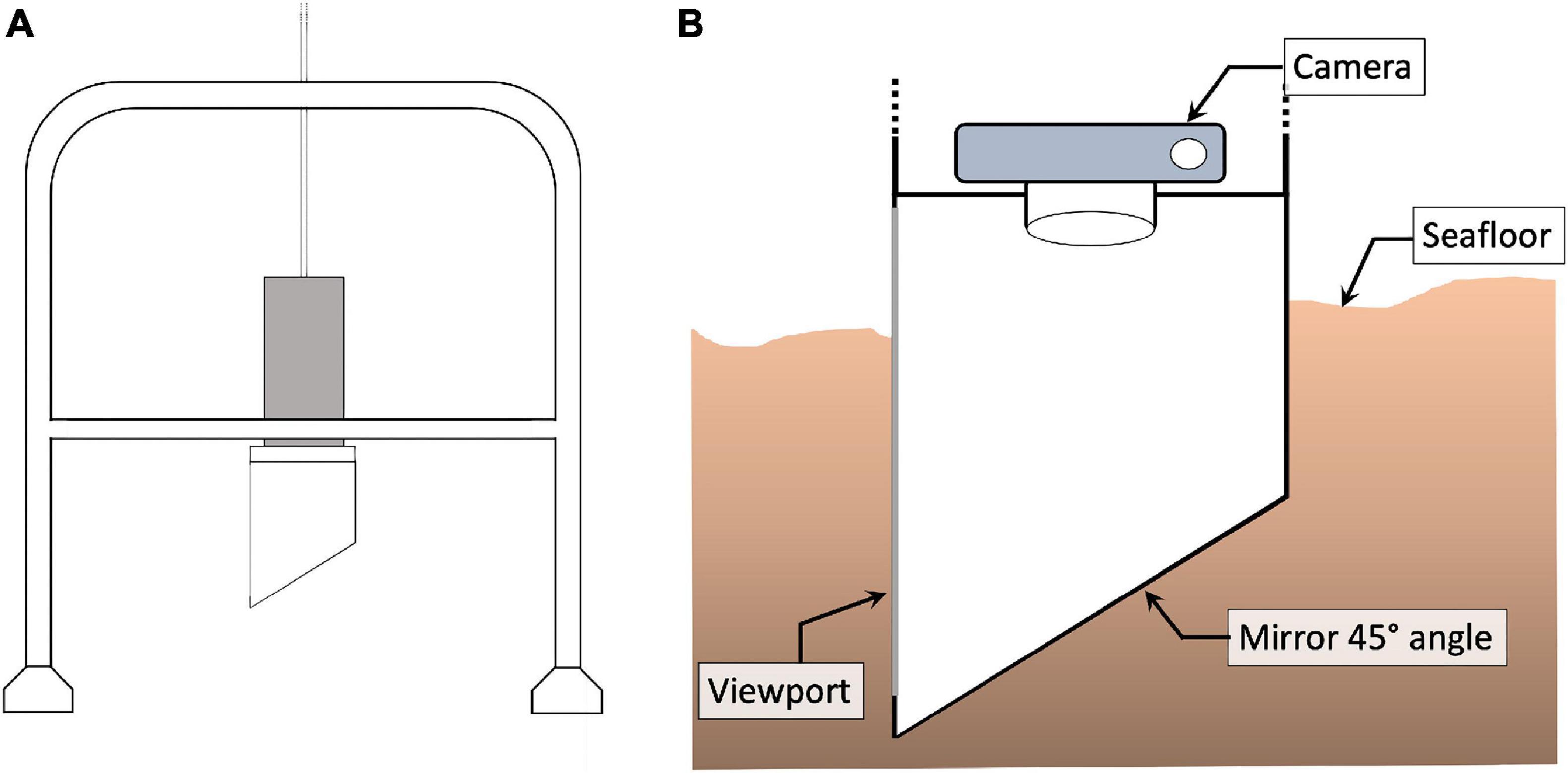
Figure 1. (A) Schematic of the SPI camera lander system. (B) Close up view of a SPI camera inserted into the sediment at the seafloor with a downward-looking camera, 45-angled mirror and viewport allowing to see the water-sediment interface.

As a result of the ability to rapidly identify benthic conditions with the SPI-camera, this cheaper and more efficient method soon became widely utilised for assessing benthic community health (Rhoads and Germano, 1982; Germano et al., 2011). Nowadays, the SPI system is used to assess the impact of aquaculture (Karakassis et al., 2002; Mulsow et al., 2006; Callier et al., 2008), trawling (Rosenberg et al., 2003), sewage effluent (Makra et al., 2001), and oil spills (Germano, 1995; Rhoads et al., 1995) on the benthos. Furthermore, the SPI system is a recommended method for assessing the quality of benthic environments for marine spatial management and environmental decision-making (O’Connor et al., 1989; Rosenberg et al., 2009).

While the SPI-camera has been widely used in marine monitoring studies for decades, significant artefacts may be associated with the technique, and the interpretations of pictures taken with a SPI system can be problematic for some sediment types (Rosenberg et al., 2001). For example, Santner et al. (2015) showed that inserting a flattened sediment corer caused considerable particle displacement from the top layer to deeper sediment layers by a process called smearing. SPI alternatives have been developed, for example by Patterson et al. (2006) who developed an inexpensive scanner-based SPI system that was of a smaller width and penetrated deeper into the sediment. Furthermore, Blanpain et al. (2009) developed a dynamic SPI system (DySPI) to conduct experiments in habitats where the use of a SPI camera is limited such as in coarse sediments. The DySPI system penetrates the sediment horizontally to ensure an undisturbed water-sediment interface.

Since SPI systems are a commonly used commercial and scientific tool, it is important to know the strengths and weaknesses of the system to be able to critique the data gathered and to be able to make informed management decisions. In this study, we developed a laboratory-scale experimental chamber called the SPI purpose-built sediment chamber (SPI-PUSH) to investigate and quantify how sediment particles are pushed downwards into deeper layers when a flat viewport penetrates the sediment which will also happen during a SPI-deployment. Although, the SPI-PUSH did not fully simulate a SPI camera penetration (e.g., in terms of the viewports size, material and the force of penetration), it provided a first assessment of the amount of smearing that may occur during a SPI survey. A variety of sediment types were used in the study including sandy sediments and soft-muddy sediments as well as luminophores (dyed inert sediment particles) of different grain sizes to visually assess the extent of the smearing. We hypothesised that “the median penetration depth of particles would be significantly greater when a flat bevelled plate penetrates the sediment compared to a control situation, where the flat bevelled plate was inserted before sediments and luminophores were added to the chamber of the SPI-PUSH.”

Materials and Methods

Purpose-Built Sediment Chamber

We developed the SPI purpose-built sediment chamber (SPI-PUSH), illustrated in Figure 2, to assess the impact of a flat bevelled plate being inserted into the sediment. The SPI-PUSH comprised 2 half chambers (Figure 2A, green and orange parts) which allowed a bevelled (45°) acrylic plate of 3 mm thickness to be inserted between them (Figure 2A, yellow plate). The device was able to be sealed, using black rubber gasket sheets between (a) the 2 halves of the main chamber between the orange plate holders (Figure 2B), (b) the chamber and the 2nd base plate, and (c) the 2nd and 1st base plate (Figure 2A, gasket sheets not shown).

FIGURE 2

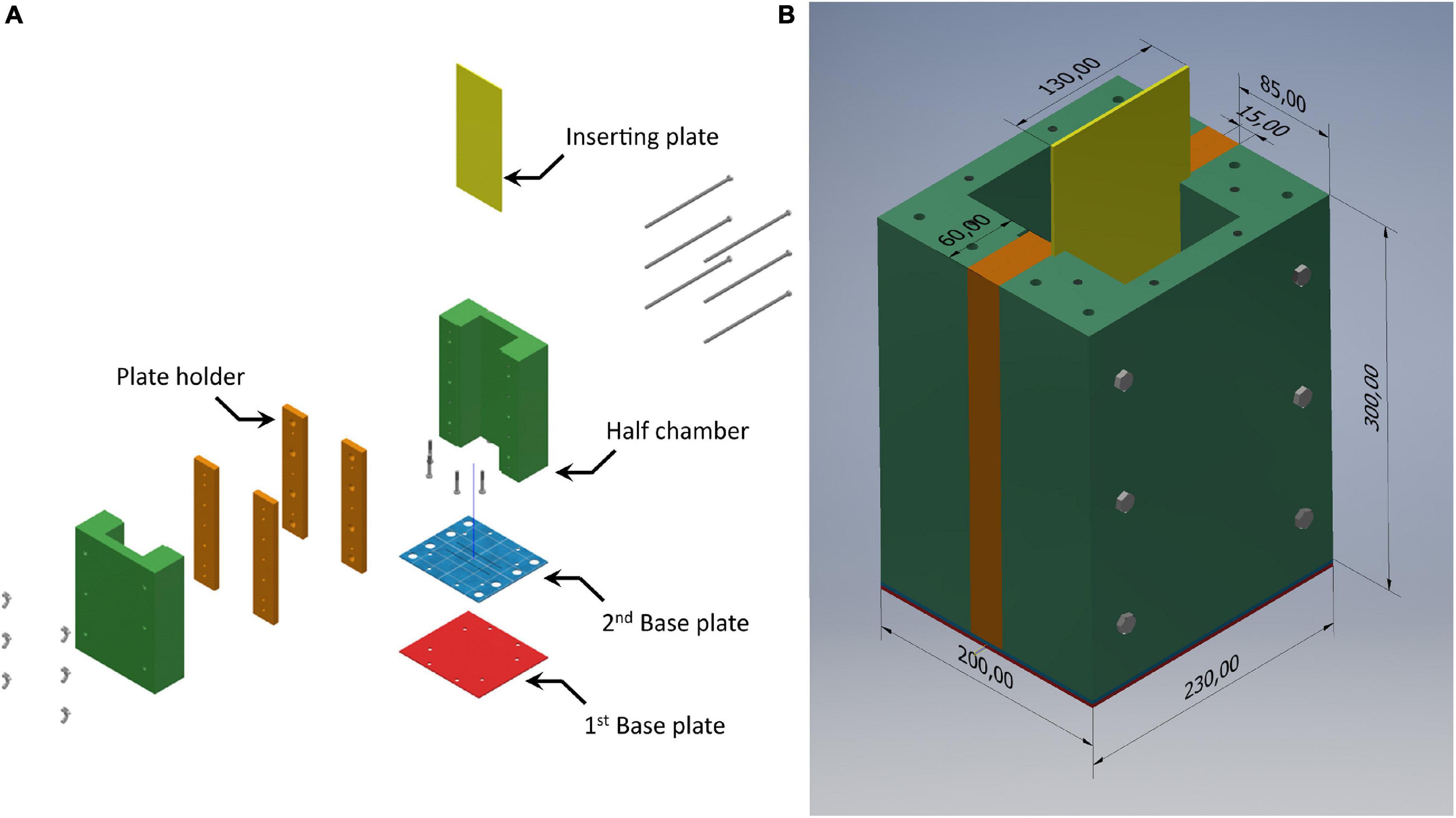
Figure 2. (A) Assembly diagram of the SPI-PUSH. Both half chambers (green) and the plate holder (orange) can be joined to form one chamber. Both base plates and gaskets (not shown) seal the bottom of the chamber. The half chamber (green) and the plate holder (orange) create a groove to insert the bevelled plate (3 mm) (yellow) (B) SPI-PUSH assembled. Dimensions shown are in mm.

Sampling and Sediment Characteristics

Sediment was sampled from the RV “Serpula” at 2 sites in Ardmucknish Bay north of Oban, Scotland (Figures 3A,B). A Van-Veen grab (0.1 m²) was used to sample subtidal sediments at two sites in September 2018, while a third intertidal site in Ardmucknish Bay was sampled with a spade in November 2019 (Figure 3C). Immediately after sampling, all sediment was sieved through a 300 μm mesh to remove all macrofauna and larger meiofaunal taxa to reduce bioturbation effects so that all particle movement in the experimental chambers could be attributed to the insertion of the plate. Sediments were then covered with aerated seawater and stored at 15°C for at least 3 months to allow the recovery of sediment biogeochemical characteristics back to in situ conditions as much as possible.

FIGURE 3

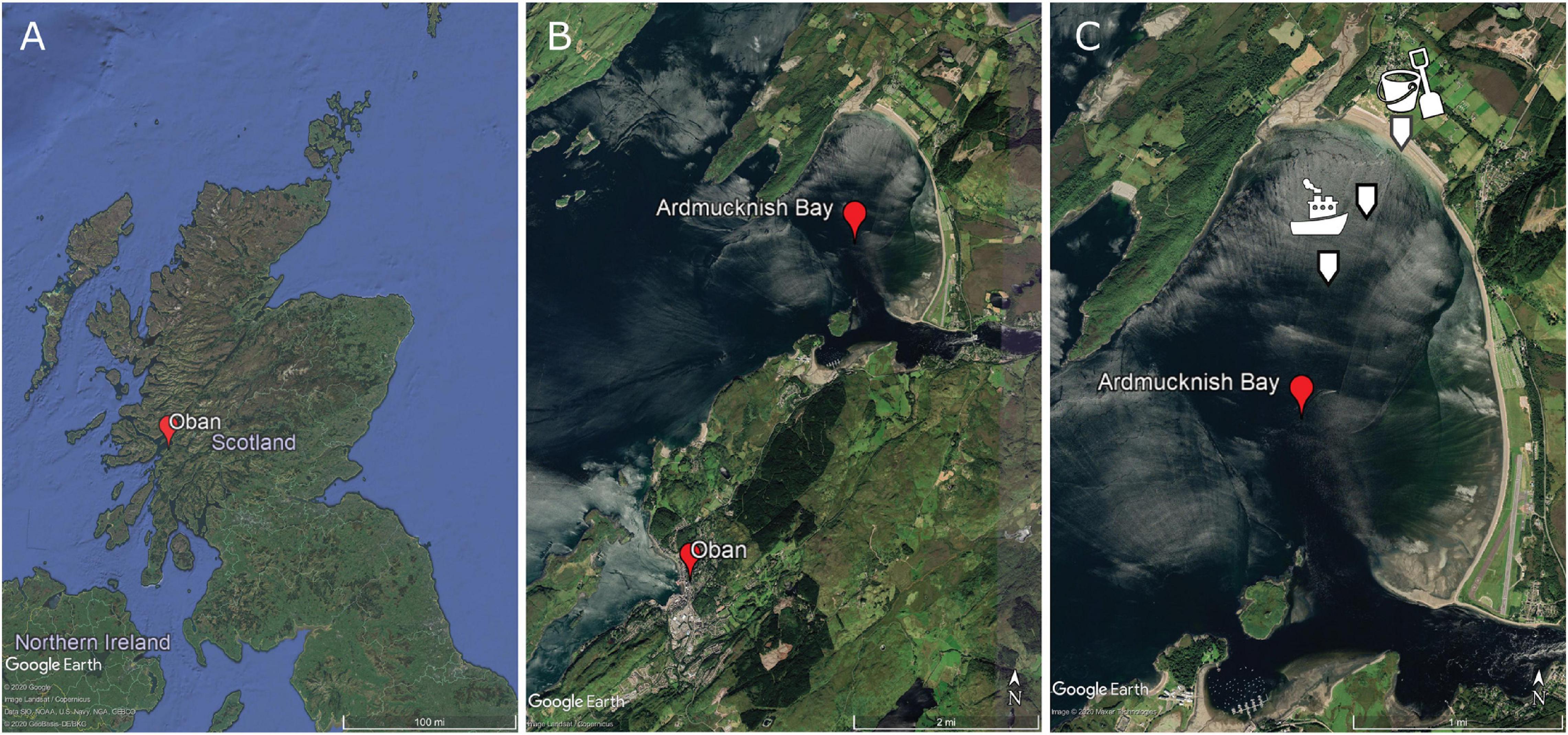
Figure 3. (A) Sampling site location within Scotland. (B) Close up view of Ardmucknish Bay north of Oban, Scotland. (C) Location of the three sites is indicated with white arrows. Pictograms illustrate the mode of sampling; the boat represents the sampling with the Van-Veen grab. ©Google Earth.

Particle Displacement Experiments

In the penetration (PEN) experiments, the SPI-PUSH was first filled with sediment to a depth of 20 cm and topped up with tap water (0.8 ± 0.2 litres, mean ± SD). Three different sediment types were used during the experiment, including mud (φ = 88 μm), fine sand (φ = 154 μm) and medium sand (φ = 187 μm) (Figure 4A). After the sediment was added to the SPI-PUSH, the sediment was allowed to settle for 1 h (sandy sediments) and 6 h (muddy sediments). To track particle displacement, inert fluorescent-dyed particles (pink, density: 2.65 g cm^–3 Partrac Ltd., United Kingdom) were used. According to the different sediments, two different luminophore sizes were used: mud-like luminophores (φ = 95 μm) were used with medium sand sediments and sand-like luminophores (φ = 177 μm) were used with both mud sediments and fine sand sediments (Figure 4B). Luminophores (34.5 ± 0.2 g, mean ± SD) were spread evenly over the topwater in the SPI-PUSH. Even distribution was ensured by a constant water current created by an aeration stone positioned above the sediment which also ensured that sediment disturbance was minimised. The luminophores were allowed to settle for 30–60 min. The impact of a flat plate penetrating the sediment was then simulated in the penetration (PEN) experiments by lowering a 3 mm thick bevelled acrylic plate into the SPI-PUSH (Figure 2, yellow). More force was required to lower the plate into medium sand sediments compared to muddy sediments. Afterward, the overlying water was drained ensuring the sediment surface was not disturbed and during this process, only a small quantity of luminophores was drained with the overlying water. The two halves of the SPI-PUSH were then separated, which allowed a cross-sectional view of the inserted plate and the degree of smearing. Two different approaches were used to determine the smearing caused by the plate: (1) an assessment of the smearing directly at the inserted plate using pictures taken at the front of the plate (see section “Smearing Directly at the Plate”) and (2) sectioning of the sediment to determine the average luminophore concentration as a function of depth and distance into the sample from the plate (see section “Averaged Sediment Smearing”). The control experiments (CNTRL) were conducted in the same way as above, except that the plate was lowered to the base of the chamber before filling the SPI-PUSH with sediments and luminophores.

FIGURE 4

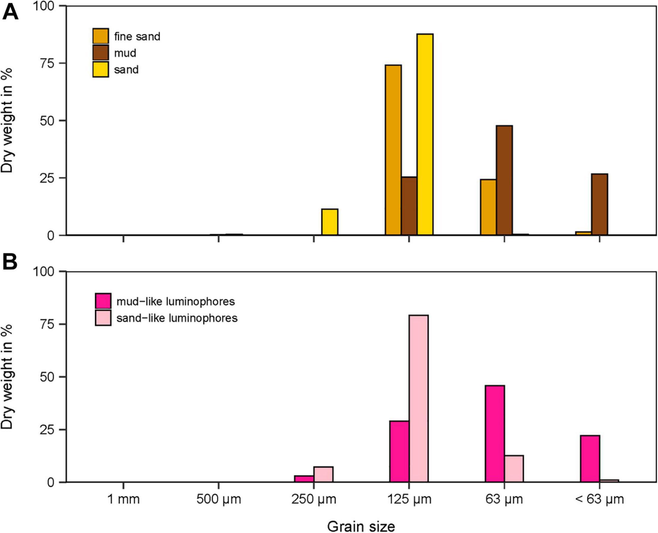
Figure 4. (A) Grain size distribution in dry weight (DW) in% of the three different sediments and (B) the luminophores used.

Smearing Directly at the Plate

Smearing of luminophores directly at the plate was photographed using a Canon EOS 50D camera (Canon EF 50 mm, f/1.8 STM Lens, with UV blocking filter) under UV light (BeamZ Flatpar 186 UV, 35 W). The height of the sediment surface from the base of the SPI-PUSH was averaged as it was not a uniform, flat surface. To do this, the width of the visible sediment column was divided into 1-cm sections, and the depths where luminophores were present was recorded for each section (Figure 5). For each experiment, 10 luminophore depth measurements were taken, and the mean and standard deviation were calculated (Figure 5).

FIGURE 5

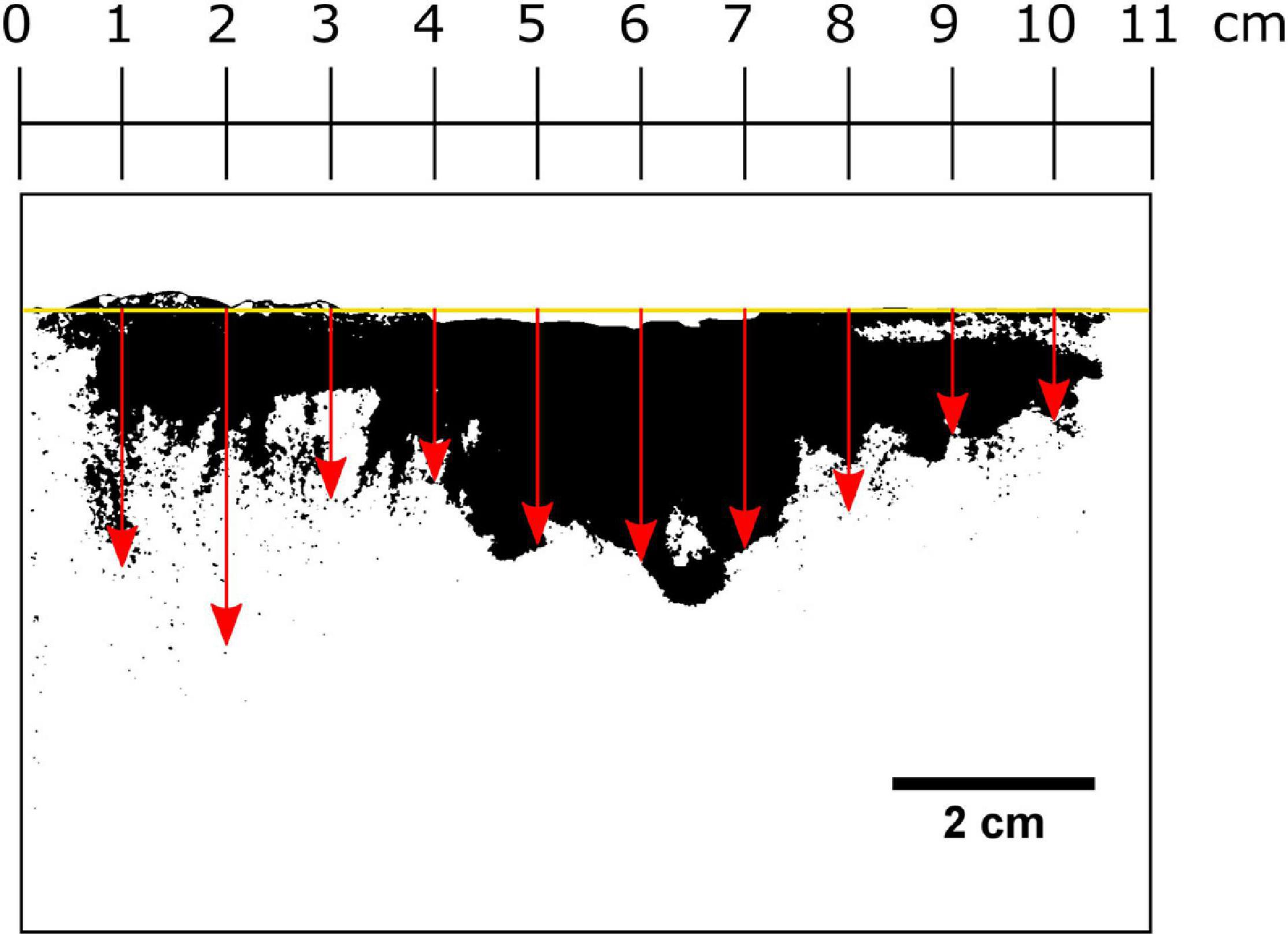
Figure 5. Procedure for determining the smearing extent directly at the inserted plate. The average height of the sediment surface was determined (yellow line) and the width of the visible sediment column was divided into vertical 1-cm intervals. The depth in which luminophores were present at each centimetre was recorded indicated here by red arrows.

Averaged Sediment Smearing

After photographing the extent of smearing at the plate (see section “Smearing Directly at the Plate”), the SPI-PUSH was placed into a −80°C freezer for 1.5 h. The sediment and SPI-PUSH were then removed, and the sediment block was cut into horizontal layers of 0–1 cm, 1–2 cm, 2–3 cm, 3–4 cm, 4–5 cm, 5–7 cm, 7–10 cm and > 10 cm (Figure 6). Each layer was divided into the portion of sediment situated 1 cm from the plate (hereafter termed FRONT) and a portion of sediment situated 1 cm behind the plate to the back edge of the chamber (hereafter termed BACK) (Figure 6). The smallest vertical and horizontal unit of 1 cm was chosen for accuracy and to avoid sampling artefacts such as particle smearing induced by cutting sediment layers. Each sediment sample was then thawed and homogenised in a sampling bag before a sub-sample was taken and freeze-dried for ∼ 48 hrs. The number of luminophores at each depth and position (FRONT and BACK) were then determined by transferring the freeze-dried sediment (0.5 g) into a petri dish (Ø 5.5 cm), photographing the dish and sediments under UV light and counting the luminophore particles using the Image analysis software ImageJ (Schneider et al., 2012). In every replicate the percentage of the luminophores was calculated from the proportion of the overall luminophore weight added and particles found at each depth and position.

FIGURE 6

Figure 6. Sediment sectioning. Sediment was vertically sectioned into the front (0–1 cm from the plate) and the back (1–5.5 cm) of the SPI-PUSH. Horizontally the sediment was cut into 1 cm slices at the top (0–5 cm) and bigger slices at the bottom (5 to >10 cm) of the chamber. Pink numbers represent the respective numbers used in figures below.

Sediment Characteristic Measurements

Sediment density, water content and porosity were determined after the experiment had been conducted by first sectioning the sediments with a clean knife, weighing the sediment slice and then freeze-drying the horizontal sediment layers (0–1 cm, 1–2 cm, 2–3 cm, 3–4 cm, 4–5 cm, 5–7 cm, 7–10cm and > 10 cm) (see section “Averaged Sediment Smearing”) for at least 48 h using a Christ Alpha 1–4 LD plus freeze-dryer. The density and water content were then calculated according to Kenny and Sotheran (2013). Loss on ignition (LOI) was determined using the protocol of Heiri et al. (2001). Grain size distribution was determined by particle size analysis whereby each sediment sample was first dried at 90°C for a minimum of 24 h. Afterward, the sediment was disaggregated with 6% aqueous sodium hexametaphosphate and soaked for 12 h (Kenny and Sotheran, 2013; Egessa et al., 2020). The < 63 μm fraction was then wet sieved and both parts (<63 μm and >63 μm) were dried at 90°C until a constant weight was achieved. The >63 μm part of the sediment was then dry sieved for 15 min through a sieve stack (1 mm, 500 μm, 250 μm, 125 μm, and 63 μm) (Folk and Ward, 1957; Blott and Pye, 2001). The weight for all fractions was then recorded.

Statistical Analyses

The median depth of smearing directly at the plate in the CNTRL and PEN experiments for each sediment and luminophore type was analysed using a non-parametric Mann-Whitney U-test as both raw and transformed datasets failed parametric assumptions. An alpha level of <0.05 was used as the criterion for statistical significance. All data analyses were done using IBM SPSS Statistics 26 software (IBM Corp, 2017).

Results

Sediment Characteristics

The grain size distribution of the mud, fine sand and medium sand had a median φ of 88, 154, and 187 μm, respectively (Figure 4A). The water content of the mud, fine sand and medium sand was 34 ± 0.4%, 25 ± 0.4%, and 25 ± 0.8% (mean ± SD), respectively, which coincided with a sediment density for mud, fine sand, and medium sand of 1.7 ± 0.04 g cm^–3, 1.8 ± 0.004 g cm^–3, and 1.8 ± 0.1 g cm^–3 (mean ± SD), respectively (Table 1). The porosity for mud and fine sand ranged between 0.58 (mud) and 0.46 (fine sand) and the organic content was 2.87 ± 0.1% for mud, 1.3 ± 0.2% for fine sand and 0.97 ± 0.2% for medium sand (mean ± SD, Table 1).

TABLE 1

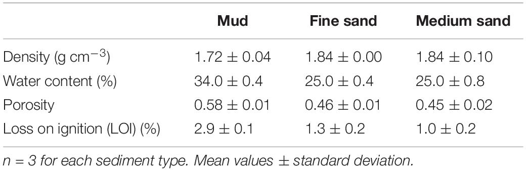
Table 1. Mean density, water content, loss on ignition and porosity values for mud, fine sand, and medium sand.

Particle Smearing Experiments

Smearing Directly at the Plate

Within all of the experiments, luminophores in the control treatment were found to be restricted to a thin layer on the top of the sediment (Figure 7), with a mean particle penetration depth of 0.1 cm recorded for mud and sand-like luminophores (Figure 8A), 0.4 cm for fine sand and sand-like luminophores (Figure 8B), and 0.6 cm for medium sand and mud-like luminophores (Figure 8C). The mean depth of particle displacement directly at the inserted plate averaged 2.9 ± 1.5 cm (mean ± SD) for mud with sand-like luminophores (Figure 8A), 4.3 ± 2.5 cm (mean ± SD) for fine-sand and sand-like luminophores (Figure 8B) and 1.9 ± 1.1 cm (mean ± SD) for medium sand and mud-like luminophores (Figure 8C). The median smearing depth differed significantly between the CNTRL and PEN treatments for mud Mann-Whitney U, n = 35, U = 182, p < 0.001), fine sand (Mann-Whitney U, n = 35, U = 182, p < 0.001) and medium sand (Mann-Whitney U, n = 35, U = 453, p < 0.001).

FIGURE 7

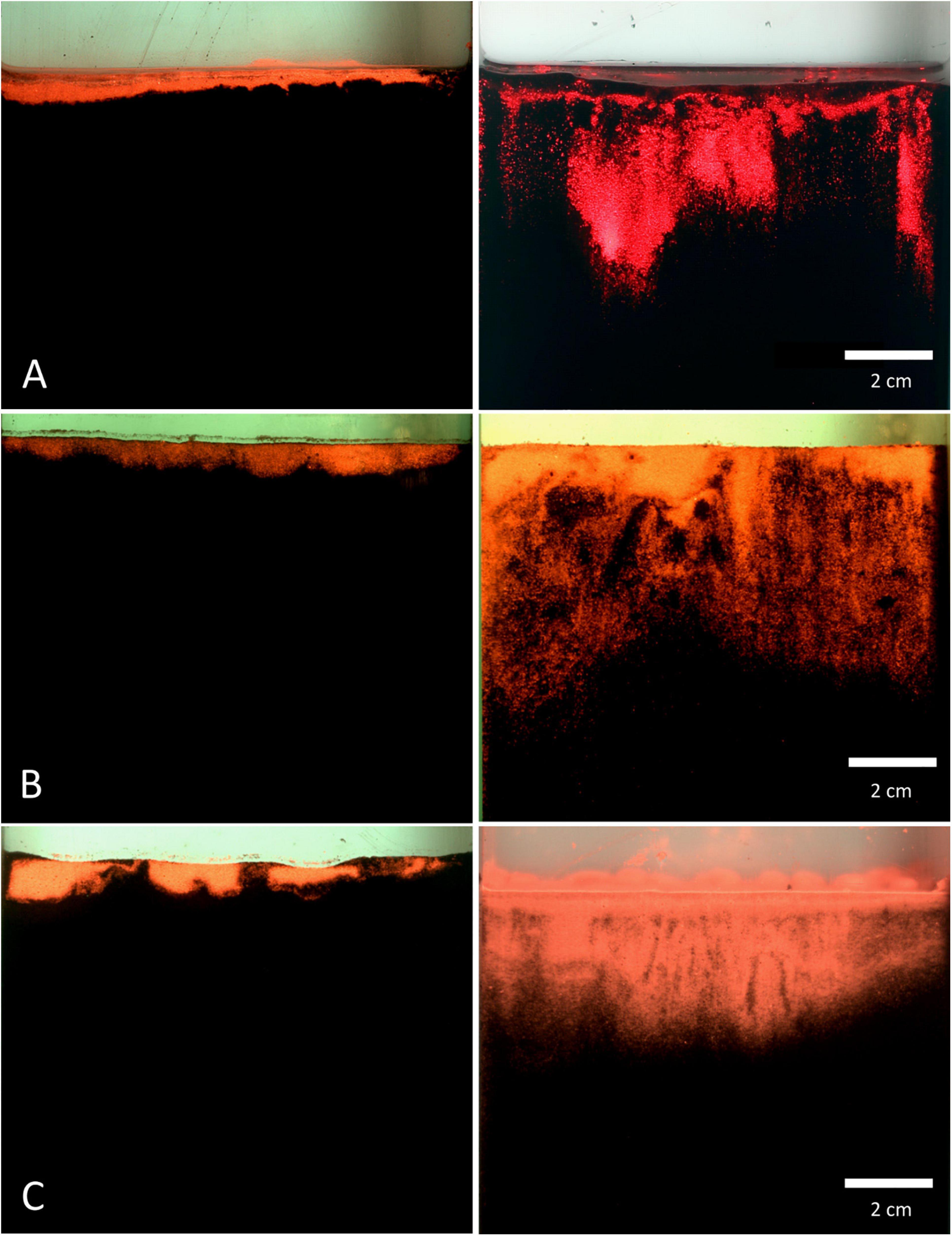
Figure 7. Pictures of the luminophore smearing directly at the inserted plate for control (left) and penetration (right) treatments. (A) mud and sand-like luminophores, (B) fine sand and sand-like luminophores, and (C) medium sand and mud-like luminophores. Image colours are digitally enhanced to simplify interpretation.

FIGURE 8

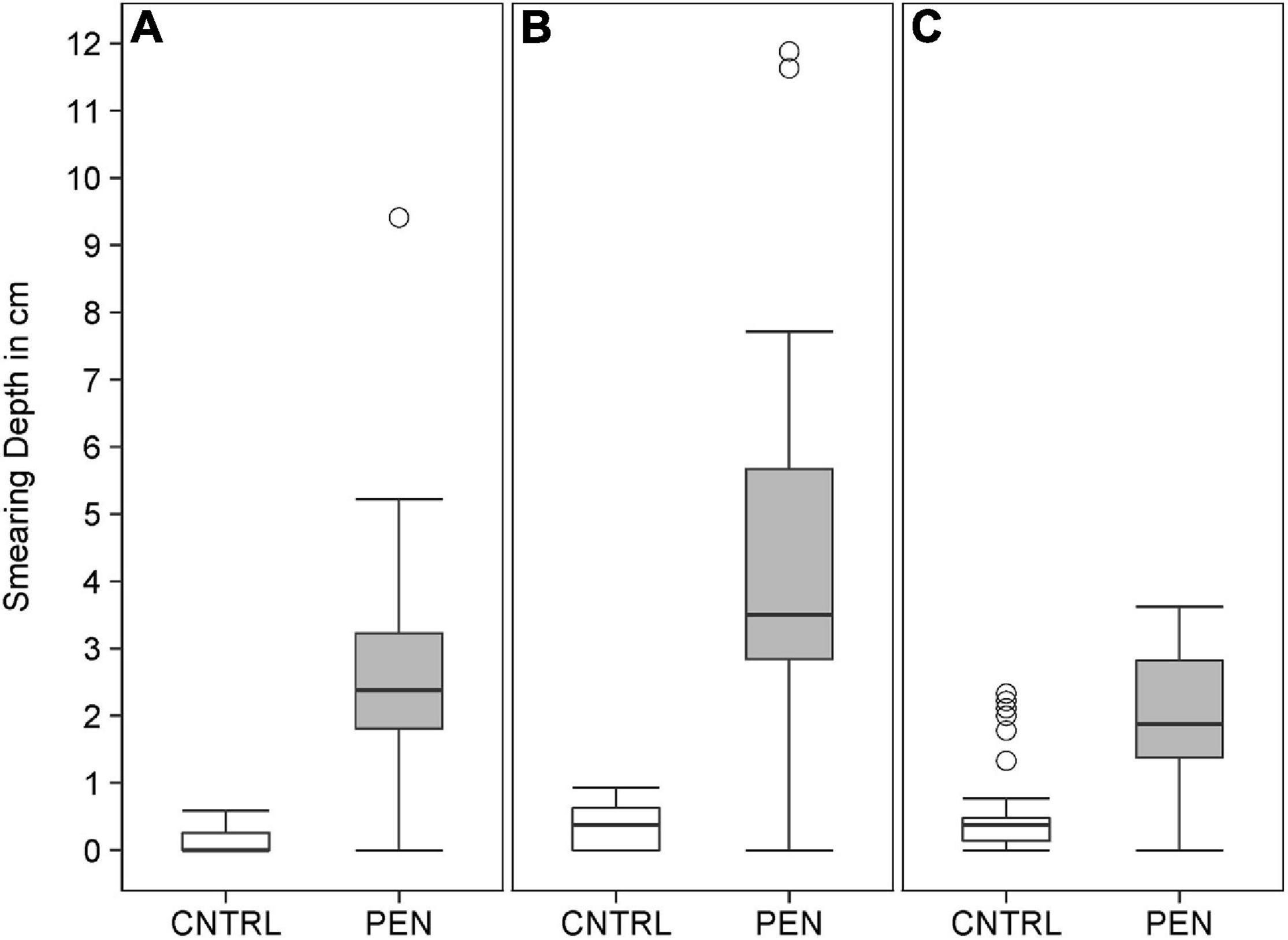
Figure 8. The depth of luminophore smearing directly at the inserted plate for (A) mud and sand-like luminophores, (B) fine sand and sand-like luminophores, (C) and medium sand and mud-like luminophores in the control (CNTRL) and penetration (PEN) treatment. The box represents the interquartile range, the median is indicated by a line within the box. Whiskers indicate variability outside the interquartile range and circles indicate outliers.

Averaged Smearing in Sediment Compartments

In the CNTRL experiments, most luminophore particles added to the FRONT were mainly confined to the surface layer (0–1 cm) for all sediment types (Figures 9–11A). However, 21% of the luminophores were found within the second centimetre for the mud and sand-like luminophore experiments (Figure 9A) and 5% were found between 3 and 4 cm for the medium sand and mud-like luminophore treatment (5%) (Figure 10A). This might reflect artefacts associated with handling and sampling these experiments.

FIGURE 9

Figure 9. Luminophore distribution (%) as a function of sediment depth (cm) in the mud sediment experiments with sand-like luminophores. (A) Front close to the plate for the CNTRL and PEN treatment. (B) Toward the back of the sediment for the CNTRL and PEN treatment. The box represents the interquartile range, the median is indicated by a line within the box. Whiskers indicate variability outside the interquartile range and circles indicate outliers.

FIGURE 10

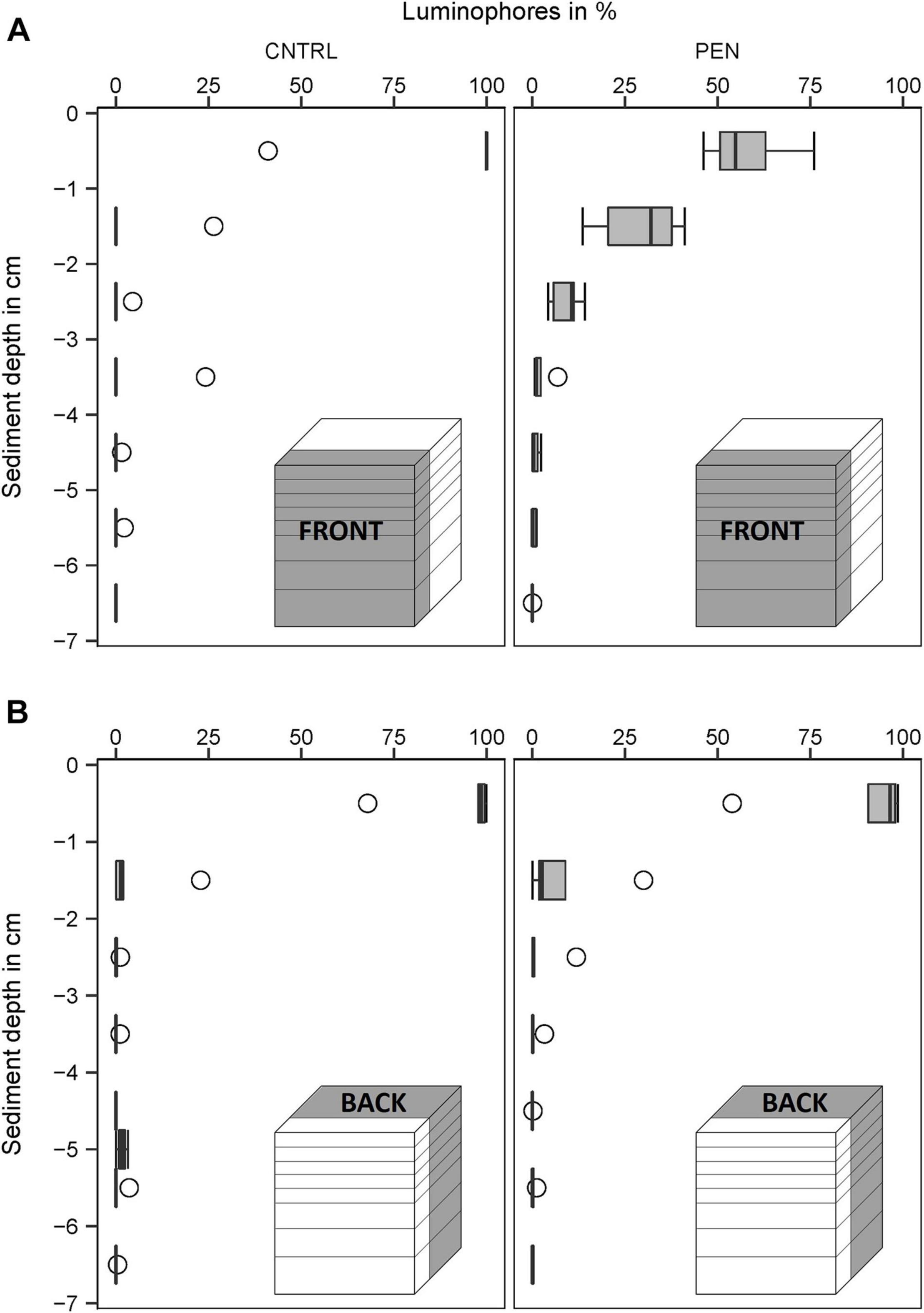
Figure 10. Luminophore distribution (%) as a function of sediment depth (cm) in the fine sand experiments with sand-like luminophores. (A) front close to the plate for the CNTRL and PEN treatment. (B) Toward the back of the sediment for the CNTRL and PEN treatment. The box of the boxplot represents the interquartile range, the median is indicated by a line within the box. Whiskers indicate variability outside the interquartile range and circles indicate outliers.

FIGURE 11

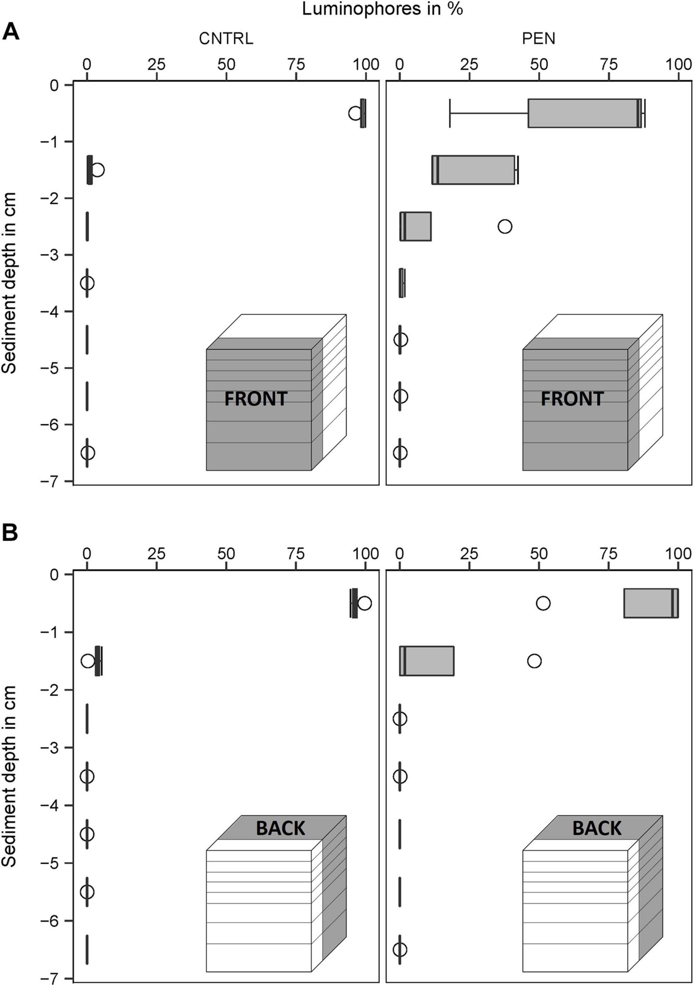
Figure 11. Luminophore distribution (%) as a function of sediment depth (cm) in medium sand with mud-like luminophores. (A) front close to the plate for the CNTRL and PEN treatment. (B) Toward the back of the sediment for the CNTRL and PEN treatment. The box of the boxplot represents the interquartile range, the median is indicated by a line within the box. Whiskers indicate variability outside the interquartile range and circles indicate outliers.

In contrast, in the PEN experiments, considerable smearing of luminophore particles occurred after inserting the plate into the sediment. Only 42% (1) (Figure 9A), 58% (2) (Figure 10A), and 65% (3) (Figure 11A) of the added luminophores were found at the sediment surface after the insertion procedure. 40% (Figure 9A), 29% (2) (Figure 10A), and 24% (3) (Figure 11A) of the luminophores initially added were subducted between 1 and 2 cm depth, and 15% (1) (Figure 9A), 9% (2) (Figure 10A), and 10% (3) (Figure 11A) of the added luminophores (6 g) were observed between 2 and 3 cm depth at the FRONT in the (1) mud and sand-like luminophores, (2) fine sand and sand-like luminophores, and (3) medium sand and mud-like luminophores, respectively. The median penetration depth of the luminophore particles at the FRONT differed significantly between the two treatments for all sediment types (Figures 9–11A) (Mud and sand-like luminophores: Mann-Whitney U, U = 378, p = 0.009, n = 35; fine sand and sand-like luminophores: Mann-Whitney U, U = 324, p = 0.001, n = 35; medium sand and mud-like luminophores: Mann-Whitney U, U = 407, p = 0.015, n = 35).

For the BACK section, luminophores were mainly found at the top of the sediment and the penetration depth of them did not significantly differ from the control nor between the different sediment types (Figures 9–11B) (Mud and sand-like luminophores: Mann-Whitney U, U = 471, p = 0.09, n = 35; fine sand and sand-like luminophores: Mann-Whitney U, U = 469, p = 0.13, n = 35; medium sand and mud-like luminophores: Mann-Whitney U, U = 542, p = 0.39, n = 35).

Discussion

SPI systems have been used for over 50 years to examine the quality of benthic environments in areas exposed to anthropogenic disturbance (Rhoads and Cande, 1971; Nilsson and Rosenberg, 1997; Germano et al., 2011; Oug et al., 2011; Sweetman et al., 2014). During this time, many researchers have shown that SPI systems displace upper-sediment particles to deeper sediment depths and in doing so, most likely drag oxygenated sediments and smear bioturbation features to deeper depths. However, surprisingly we know of no other study that has assessed the extent of smearing in different sediment types nor if sediment smearing is a localised phenomenon that only occurs next to the glass plate of a SPI. In this study, we designed a lab-based experiment that simulated the penetration of a flat bevelled plate into sediment and allowed us to quantify the degree of smearing. Although an actual SPI system was not used due to their size and weight precluding a controlled laboratory study and therefore limits the extrapolation of our results to real SPI surveys, the experiment was successful in providing a first-order approximation of the amount of the smearing that may occur with a SPI system. Our experiments showed that the penetration of a flat surface into different sediment types generates significant smearing and displaces surface sediment particles to depths of 3–4 cm adjacent to the plate. This supports our hypothesis that the median penetration depth of particles is significantly greater when a flat plate penetrates the sediment compared to in a control experiment. Our findings, therefore, suggest that smearing over cm-scales may occur during SPI camera surveys and possibly makes anthropogenically disturbed habitats appear healthier than they are.

Although a real SPI was not used in this study and the sediment was sieved to remove fauna which likely impacted its texture and structure and means that the results may differ to in situ situations, the results were consistent with images from SPI-camera surveys where clear smearing has been shown. Santner et al. (2015) previously suggested that lowering a periscope-like device, such as the SPI into marine sediments leads to particle smearing and this might also have an effect on the porewater chemistry, which has been shown experimentally using planar optode devices that also feature a periscope-penetration system (Glud et al., 2001). However, due to fast oxygen consumption rates in deep, poorly oxygenated cohesive sediments, the importance of porewater smearing is usually considered minor, especially if enough time is allowed for porewater conditions to re-establish before taking pictures. Methods such as planar optodes, oxygen microelectrodes or DET/DGT (diffusive equilibration/gradients in thin films) are not limited to measuring oxygen concentrations but are available for measuring a range of solutes and conditions such as pH and H₂S, thus allowing a set of alternative methods for assessing benthic health and avoiding smearing artefacts (Revsbech et al., 1983; Glud et al., 2005; Fan et al., 2011; Almroth-Rosell et al., 2012; Cathalot et al., 2015; Santner et al., 2015). However, information from microelectrodes can sometimes be limited due to the small area measured and their fragility. Regular monitoring of the sediment with a more comprehensive toolbox of non-SPI methods would, however, reduce possible experimental artefacts created by SPI systems (as suggested by our data) though this might not be possible due to time and cost constraints (Rhoads and Young, 1970; Germano et al., 2011).

The deepest smearing that was observed in experiments using fine sand sediments with sand-like luminophores was 4.25 ± 2.5 cm. Providing these results are consistent with actual SPI systems used in situ, they suggest that surface sediments could be subducted many centimetres below the sediment-water interface and drastically complicate interpretations of any images collected during SPI seafloor surveys in fine sandy environments (Rosenberg et al., 2009; Grant, 2010; Norkko et al., 2019). The deep penetration of the luminophores in the fine sand experiments relative to the mud-sediment experiments may be explained by the difficulties in lowering the plate into the SPI-PUSH, compared to the muddy sediment treatment (Bradley and Morris, 1990; Germano et al., 2011). However, experiments with medium sand and mud-like luminophores, showed considerably shallower smearing even though the same difficulties associated with lowering the plate arose. The size of the luminophores and sediment particles may have influenced their behaviour and impacted the depth of smearing. Small luminophore and sediment particles have a high surface tension, which can lead to cohesive particles attaching themselves to other sediment particles as well as the SPI-PUSH housing (Nichols, 2009). If this was a factor in our experiments, the experiments with the smallest sized luminophores (e.g., the mud-like luminophores) should have displayed the deepest particle displacement yet it was fine sand and the sand-like luminophore experiments that showed the deepest smearing. In future experiments aimed at measuring smearing effects, we suggest that the luminophore particle sizes should match the ambient sediment grain size so that the luminophores behave as naturally as possible and in a similar manner to the ambient sediments present enabling one to quantify the real extent of smearing.

In these experiments, two different approaches were used to assess the extent of smearing. These included taking pictures directly at the front plate of the SPI-PUSH and documenting the mean depth of luminophore penetration (approach 1). The second approach involved collecting sediments from individual layers and counting the number of luminophores in each depth layer and comparing this to the amount deposited at the sediment surface. The mean smearing depth at the front of the plate using the first approach was 2.7 cm for mud and sand-like luminophores and 1.9 cm for medium sand and mud-like luminophores. This data was consistent with the data measured in the second approach, with 54% of the luminophores found in 2–3 cm at the front of the plate in the mud experiments, and 89% of the luminophores found between 1 and 2 cm depth at the front of the plate in the medium sand experiments. Based on this first approach, the mean depth of particle smearing at the plate was 4.3 cm, whereas the second approach showed that 97% of the luminophores were found in the first two centimetres of the sediment. The discrepancy between the two approaches may occur due to analysing the averaged sediment volume (second approach) compared to the thin sediment layer directly at the plate (first approach). In the second approach, sediment particles further away from the plate might be impacted less by the insertion. This may explain the lower percentage of found luminophores compared to the first approach. This highlights the importance of using both approaches to compensate for any potential artefacts associated with the experimental design or the SPI-PUSH. Nevertheless, both approaches suggest significant smearing arise from a flat bevelled plate being inserted into the sediment, which suggests smearing studies be conducted in situ with real SPI systems in future. In addition to smearing being observed immediately at the plate (approach 1), the penetration of the luminophores (approach 2) was also detected at a depth between 1 and 2 cm, 2–5 cm away from the inserted plate for all sediment types and penetration experiments though this was not significant and possibly related to the lower statistical power inherent in non-parametric statistical tests. Although the penetration of particles at positions situated away from the plate could be caused by the compressibility of the sediment as documented by Bradley and Morris (1990), less sediment was subducted to deeper sediment depths in the CNTRL compared to the PEN experiments at the back of the SPI-PUSH which points to possible near and far-field smearing effects, which should possibly be studied with real SPI-systems in greater detail. We also recommend that future studies trying to document how significant lateral smearing is, would be to sample several successive lateral zones from the plate (e.g., each 2–5 mm) as this may give a better understanding of the lateral mixing (i.e., how far from the plate is the influence detectable), and, as in this study, the sediments be frozen prior to cutting into several lateral layers to limit luminophore movement.

Data collected by SPI cameras are regularly used to generate a Benthic Habitat Quality (BHQ) index, to determine the health of a specific site in the context of the European Water Framework Directive that aims to assess, monitor and, if applicable, improve all European rivers, lakes, and coastal waters (Anonymous, 2000; Kallis, 2001; Rosenberg et al., 2009). The BHQ depends, amongst other parameters, on the depth of the visually distinguishable apparent redox potential discontinuity (aRPD) layer. The value of the aRPD ranges between 0 and 5 depending on its depth and contributes up to 33% of the overall BHQ value with a BHQ value of 0 indicating poor benthic health, and a value of 15 indicating a good environmental status (Nilsson and Rosenberg, 1997). Because SPI cameras are often used to determine the depth of the aRPD, both the method and the BHQ are particularly vulnerable to smearing artefacts. While our experimental design did not replicate an actual SPI-system, if our results are representative for SPI systems, they suggest that surface sediments (which in natural, unpolluted settings are usually lighter and more oxygenated, e.g., Fenchel and Riedl, 1970; Sweetman et al., 2014; Statham et al., 2019) may be subducted to several centimetres depth, highlighting that the depth of the aRPD layer (and thus, the BHQ) measured by SPI surveys may be overestimated in some cases. Diaz et al. (2003) did provide evidence that SPI cameras possibly overestimated the BHQ compared to BHQ values derived by analysing macrofaunal community structure from samples collected by a Van-Veen grab. However, the authors concluded that the mismatch was due to the geographical patchiness of benthic communities rather than smearing artefacts caused by the SPI system (Diaz et al., 2003). Mulsow et al. (2006) also showed that the visually assessed aRPD and the measured RPD were incomparable in a study that assessed BHQ underneath fish farms in two southern Chilean fjords (Mulsow et al., 2006). The RPD determined using redox microelectrodes ranged between 0.4 and 1.7 cm, whereas the SPI data suggested that the aRPD was at 2–3 cm (Mulsow et al., 2006), which, based on our data, could have been because of smearing of surface sediments to deeper sediment layers. Finally, Gerwing et al. (2013) found a RPD of 4 cm on intertidal mudflats in the Bay of Fundy, Canada compared to an average aRPD of 3.3 cm, which in some instances was much deeper (between 4 and 5 cm). Overestimating the depth of the aRPD as a result of smearing artefacts created by SPI systems can lead to false benthic infaunal succession stage assessments. For example, Cicchetti et al. (2006) estimated the BHQ of a site in Narragansett Bay, RI, United States to be between 1 and 7 over the same sampling period based on the aRPD determined by sediment profile camera pictures. Based on these findings the calculated succession stage at sampling station ranged between 0 (grossly polluted) to 2 (transitory from normal to polluted) (Pearson and Rosenberg, 1978; Nilsson and Rosenberg, 2000; Cicchetti et al., 2006). An environment that is transforming from a healthy to grossly polluted state will be managed very differently under the Water Framework Directive. In Scotland, the Scottish Environment Protection Agency (SEPA) is responsible for ensuring that robust environmental monitoring of the seafloor around fish farms is undertaken (SEPA, 1998). Assuming our data is, therefore, representative of the smearing that occurs with actual SPI systems, it is possible that the environmental thresholds that are set out by SEPA/the WFD (that command deliberate actions be taken to improve ecosystems, Henderson and Davies, 2000), might be missed by using pictures generated by SPI systems. Going forward, it is now important to implement studies to assess the real smearing effect associated with SPI systems in situ and try to derive correction factors for SPI images in different sedimentary settings. This would enhance our understanding of benthic health and improve benthic habitat management.

Conclusion

This study assessed the potential impact that the penetration of a front plate from a sediment penetrating device might have on the smearing of surface sediments to deeper sediment layers. The study showed that particle subduction from surficial sediments into deeper sediment layers can be significant and varied as a function of the sediment type and the luminophores used from a mean of 1.9 ± 1.1 cm for medium sand and mud-like luminophores to 2.9 ± 1.5 cm for mud and sand-like-luminophores and 4.3 ± 2.5 cm for fine sand and sand-like luminophores measured directly at the inserted plate. If our results are representative of the actual smearing that takes place when using real SPI systems, they suggest that the data gathered with SPI-systems, if uncorrected, may lead to incorrect assumptions regarding benthic health, which could ultimately lead to inappropriate management decisions. Moving forward, it is important to test the effects of smearing with actual SPI cameras in situ using luminophores that match the grain size distribution of the sediment being visited so that correction factors can be developed for SPI cameras for use in different environmental settings. Before correction factors are established, it will be important for all future studies to acknowledge that significant smearing may occur, and that data gathered using SPI-cameras needs to be treated with caution.

Data Availability Statement

The raw data supporting the conclusions of this article will be made available by the authors, without undue reservation.

Author Contributions

AM and AS designed the study. AM generated the data and analysed the dataset. IP designed the SPI-PUSH. BN made sediment processing facilities available for the fieldwork. AM wrote the manuscript with contributions from all authors.

Funding

This work has been completed within the NEXUSS centre for Doctoral Training granted by the UK Natural Environment Research Council (NERC) (NE/N012070/1).

Conflict of Interest

The authors declare that the research was conducted in the absence of any commercial or financial relationships that could be construed as a potential conflict of interest.

Acknowledgments

We wish to thank Alastair Lyndon and the captain of the RV “Serpula” who made the fieldwork in 2018 possible. Alastair Lyndon provided advice on the statistics used in this paper. Further, thanks go to Marta Maria Cecchetto for assisting AM during fieldwork, and to Leon Pedersen (Bergen, Norway) who built the SPI-PUSH. We would also like to thank the two reviewers who provided constructive comments that helped to improve this manuscript.

References

Almroth-Rosell, E., Tengberg, A., Andersson, S., Apler, A., and Hall, P. O. J. (2012). Effects of simulated natural and massive resuspension on benthic oxygen, nutrient and dissolved inorganic carbon fluxes in Loch Creran, Scotland. J. Sea Res. 72, 38–48. doi: 10.1016/j.seares.2012.04.012

CrossRef Full Text | Google Scholar

Alongi, D. M., Mckinnon, A. D., Brinkman, R., Trott, L. A., Undu, M. C., and Muawanah (2009). The fate of organic matter derived from small-scale fish cage aquaculture in coastal waters of Sulawesi and Sumatra, Indonesia. Aquaculture 295, 60–75. doi: 10.1016/j.aquaculture.2009.06.025

CrossRef Full Text | Google Scholar

Anonymous. (2000). Directive 200/60/EC of the European Parliament and of the Council of 23 October 2000 establishing a framework for Community action in the field of water policy. Off. J. 2000:L327/1.

Google Scholar

Beukema, J. J. (1974). The efficiency of the Van Veen grab compared with the Reineck box sampler. ICES J. Mar. Sci. 35, 319–327. doi: 10.1093/icesjms/35.3.319

CrossRef Full Text | Google Scholar

Blanpain, O., du Bois, P. B., Cugier, P., Lafite, R., Lunven, M., Dupont, J., et al. (2009). Dynamic sediment profile imaging (DySPI): a new field method for the study of dynamic processes at the sediment-water interface. Limnol. Oceanogr. Methods 7, 8–20. doi: 10.4319/lom.2009.7.8

CrossRef Full Text | Google Scholar

Blomqvist, S. (1991). Quantitative sampling of soft-bottom sediments: problems and solutions. Mar. Ecol. Prog. Ser. 72, 295–304. Available online at: http://www.jstor.org/stable/24825604,Google Scholar

Blott, S. J., and Pye, K. (2001). GRADISTAT: a grain size distribution and statistics package for the analysis of unconsolidated sediments. Earth Surf. Process. Landf. 26, 1237–1248. doi: 10.1002/esp.261

CrossRef Full Text | Google Scholar

Bradley, P. M., and Morris, J. T. (1990). Physical characteristics of salt marsh sediments: ecological implications. Mar. Ecol. Prog. Ser. 61, 245–252. Available online at: http://www.jstor.org/stable/24842562.,Google Scholar

Callier, M. D., McKindsey, C. W., and Desrosiers, G. (2008). Evaluation of indicators used to detect mussel farm influence on the benthos: two case studies in the Magdalen Islands. Eastern Canada. Aquaculture 278, 77–88. doi: 10.1016/j.aquaculture.2008.03.026

CrossRef Full Text | Google Scholar

Cathalot, C., Rabouille, C., Sauter, E., Schewe, I., and Soltwedel, T. (2015). Benthic oxygen uptake in the Arctic ocean margins - A case study at the deep-sea observatory HAUSGARTEN (fram strait). PLoS One 10:e0138339. doi: 10.1371/journal.pone.0138339

PubMed Abstract | CrossRef Full Text | Google Scholar

Cicchetti, G., Latimer, J. S., Rego, S. A., Nelson, W. G., Bergen, B. J., and Coiro, L. L. (2006). Relationships between near-bottom dissolved oxygen and sediment profile camera measures. J. Mar. Syst. 62, 124–141. doi: 10.1016/j.jmarsys.2006.03.005

CrossRef Full Text | Google Scholar

Diaz, R. J., Cutter, G. R., and Dauer, D. M. (2003). A comparison of two methods for estimating the status of benthic habitat quality in the Virginia Chesapeake Bay. J. Exp. Mar. Bio. Ecol. 285–286, 371–381. doi: 10.1016/S0022-0981(02)00538-5

CrossRef Full Text | Google Scholar

Egessa, R., Nankabirwa, A., Basooma, R., and Nabwire, R. (2020). Occurrence, distribution and size relationships of plastic debris along shores and sediment of northern Lake Victoria. Environ. Pollut. 257:113442. doi: 10.1016/j.envpol.2019.113442

PubMed Abstract | CrossRef Full Text | Google Scholar

Fan, Y., Zhu, Q., Aller, R. C., and Rhoads, D. C. (2011). An In Situ Multispectral Imaging System for Planar Optodes in Sediments: examples of High-Resolution Seasonal Patterns of pH. Aquat. Geochem. 17:457. doi: 10.1007/s10498-011-9124-5

CrossRef Full Text | Google Scholar

Fenchel, T. M., and Riedl, R. J. (1970). The sulfide system: a new biotic community underneath the oxidized layer of marine sand bottoms. Mar. Biol. 7, 255–268. doi: 10.1007/BF00367496

CrossRef Full Text | Google Scholar

Folk, R. L., and Ward, W. C. (1957). Brazos River bar: a study in the significance of grain size parameters. J. Sediment. Res. 27, 3–26. doi: 10.1306/74D70646-2B21-11D7-8648000102C1865D

CrossRef Full Text | Google Scholar

Germano, J. D. (1995). “Sediment profile imaging: a rapid seafloor impact assessment tool for oil spills,” in Eighteenth Arctic and Marine Oilspill Program (AMOP) Technical seminar, (Cambridge: Cambridge University), 1271–1279.

Google Scholar

Germano, J. D., Rhoads, D. C., Valente, R. M., Carey, D. A., and Solan, M. (2011). “The use of sediment profile imaging (SPI) for environmental studies: lessons learned from the past four decades,” in Oceanography and Marine Biology: An Annual Review, eds D. J. Gibson, R. N. Atkinson, R. J. A. Gordon, J. D. M. Smith, and I. P. Hughes (Boca Raton: CRC Press), 235–298.

Google Scholar

Gerwing, T. G., Gerwing, A. M. A., Drolet, D., Hamilton, D. J., and Barbeau, M. A. (2013). Comparison of two methods of measuring the depth of the redox potential discontinuity in intertidal mudflat sediments. Mar. Ecol. Prog. Ser. 487, 7–13.

Google Scholar

Glud, R. N., Tengberg, A., Kühl, M., Hall, P. O. J., and Klimant, I. (2001). An in situ instrument for planar O2 optode measurements at benthic interfaces. Limnol. Oceanogr. 46, 2073–2080. doi: 10.4319/lo.2001.46.8.2073

CrossRef Full Text | Google Scholar

Glud, R. N., Wenzhöfer, F., Tengberg, A., Middelboe, M., Oguri, K., and Kitazato, H. (2005). Distribution of oxygen in surface sediments from central Sagami Bay, Japan: in situ measurements by microelectrodes and planar optodes. Deep Sea Res. Part I Oceanogr. Res. Pap. 52, 1974–1987. doi: 10.1016/j.dsr.2005.05.004

CrossRef Full Text | Google Scholar

Graf, G., Bengtsson, W., Diesner, U., Schulz, R., and Theede, H. (1982). Benthic response to sedimentation of a spring phytoplankton bloom: process and budget. Mar. Biol. 67, 201–208. doi: 10.1007/BF00401286

CrossRef Full Text | Google Scholar

Grant, J. (2010). Coastal communities, participatory research, and far-field effects of aquaculture. Aquac. Environ. Interact. 1, 85–93. doi: 10.3354/aei00009

CrossRef Full Text | Google Scholar

Heiri, O., Lotter, A. F., and Lemcke, G. (2001). Loss on ignition as a method for estimating organic and carbonate content in sediments: reproducibility and comparability of results. J. Paleolimnol. 25, 101–110. doi: 10.1023/A:1008119611481

CrossRef Full Text | Google Scholar

Henderson, A. R., and Davies, I. M. (2000). Review of aquaculture, its regulation and monitoring in Scotland. J. Appl. Ichthyol. 16, 200–208. doi: 10.1046/j.1439-0426.2000.00260.x

CrossRef Full Text | Google Scholar

Holmer, M., and Kristensen, E. (1992). Impact of marine fish cage farming on metabolism and sulfate reduction of underlying sediments. Mar. Ecol. Prog. Ser. 80, 191–201. doi: 10.3354/meps080191

CrossRef Full Text | Google Scholar

IBM Corp (2017). IBM SPSS Statistics for Windows. New York: IBM.

Google Scholar

Kallis, G. (2001). The EU water framework directive: measures and implications. Water Policy 3, 125–142. doi: 10.1016/s1366-7017(01)00007-1

CrossRef Full Text | Google Scholar

Karakassis, I., Tsapakis, M., Smith, C. J., and Rumohr, H. (2002). Fish farming impacts in the Mediterranean studied through sediment profiling imagery. Mar. Ecol. Prog. Ser. 227, 125–133. doi: 10.3354/meps227125

CrossRef Full Text | Google Scholar

Kenny, A. J., and Sotheran, I. (2013). “Characterising the Physical Properties of Seabed Habitats,” in Methods for the Study of Marine Benthos, ed. A. Eleftheriou (New York: John Wiley & Sons, Ltd), doi: 10.1002/9781118542392.ch2

CrossRef Full Text | Google Scholar

Makra, A., Thessalou-Legaki, M., Costelloe, J., Nicolaidou, A., and Keegan, B. F. (2001). Mapping the Pollution Gradient of the Saronikos Gulf Benthos Prior to the Operation of the Athens Sewage Treatment Plant. Greece. Mar. Pollut. Bull. 42, 1417–1419. doi: 10.1016/S0025-326X(01)00220-X

CrossRef Full Text | Google Scholar

Mulsow, S., Krieger, Y., and Kennedy, R. (2006). Sediment profile imaging (SPI) and micro-electrode technologies in impact assessment studies: example from two fjords in Southern Chile used for fish farming. J. Mar. Syst. 62, 152–163. doi: 10.1016/j.jmarsys.2005.09.012

CrossRef Full Text | Google Scholar

Nichols, G. (2009). Sedimentology and Stratigraphy. Second Edi. New York:. A John Wiley & Sons, Ltd.

Google Scholar

Nilsson, H. C., and Rosenberg, R. (1997). Benthic habitat quality assessment of an oxygen stressed fjord by surface and sediment profile images. J. Mar. Syst. 11, 249–264.

Google Scholar

Nilsson, H. C., and Rosenberg, R. (2000). Succession in marine benthic habitats and fauna in response to oxygen deficiency: analysed by sediment profile-imaging and by grab samples. Mar. Ecol. Prog. Ser. 197, 139–149.

Google Scholar

Norkko, J., Pilditch, C. A., Gammal, J., Rosenberg, R., Enemar, A., Magnusson, M., et al. (2019). Ecosystem functioning along gradients of increasing hypoxia and changing soft-sediment community types. J. Sea Res. 153:101781. doi: 10.1016/j.seares.2019.101781

CrossRef Full Text | Google Scholar

O’Connor, B. D. S., Costelloe, J., Keegan, B. F., and Rhoads, D. C. (1989). The use of REMOTS^® technology in monitoring coastal enrichment resulting from mariculture. Mar. Pollut. Bull. 20, 384–390. doi: 10.1016/0025-326X(89)90316-0

CrossRef Full Text | Google Scholar

Oug, E., Cochrane, S. K. J., Sundet, J. H., Norling, K., and Nilsson, H. C. (2011). Effects of the invasive red king crab (Paralithodes camtschaticus) on soft-bottom fauna in Varangerfjorden, northern Norway. Mar. Biodivers. 41, 467–479. doi: 10.1007/s12526-010-0068-6

CrossRef Full Text | Google Scholar

Patterson, A., Kennedy, R., O’Reilly, R., and Keegan, B. F. (2006). Field test of a novel, low-cost, scanner-based sediment profile imaging camera. Limnol. Oceanogr. Methods 4, 30–37. doi: 10.4319/lom.2006.4.30

CrossRef Full Text | Google Scholar

Pearson, T. H., and Rosenberg, R. (1978). Macrobenthic succession in relation to organic enrichment and pollution of the marine environment. Oceanogr. Mar. Biol. Annu. Rev. 16, 229–331.

Google Scholar

Revsbech, N. P., Jorgensen, B. B., Blackburn, T. H., and Cohen, Y. (1983). Microelectrode studies of the photosynthesis and O2, H2S, and pH profiles of a microbial mat1. Limnol. Oceanogr. 28, 1062–1074. doi: 10.4319/lo.1983.28.6.1062

CrossRef Full Text | Google Scholar

Rhoads, D. C., and Cande, S. (1971). SEDIMENT PROFILE CAMERA FOR IN SITU STUDY OF ORGANISM-SEDIMENT RELATIONS1. Limnol. Oceanogr. 16, 110–114. doi: 10.4319/lo.1971.16.1.0110

CrossRef Full Text | Google Scholar

Rhoads, D. C., and Germano, J. D. (1982). Characterization of Organism-Sediment Relations Using Sediment Profile Imaging: an Efficient Method of Remote Ecological Monitoring of the Seafloor (Remots^TM System). Mar. Ecol. Prog. Ser. 8, 115–128.

Google Scholar

Rhoads, D. C., Valente, R., Germano, J. D., Hilbig, B., Hodgson, G., and Evans, N. (1995). “). REMOTS monitoring of dredging, disposal, sand mining, and organic enrichment on the Hong Kong shelf,” in OCEANS ’95. MTS/IEEE. Challenges of Our Changing Global Environment. Conference Proceedings, Vol. 2, (New Jersey: IEEE), 918–924. doi: 10.1109/OCEANS.1995.528539

CrossRef Full Text | Google Scholar

Rhoads, D. C., and Young, D. K. (1970). The influence of deposit-feeding organisms on sediment stability and community trophic structure. J. Mar. Res. 28, 150–178.

Google Scholar

Rosenberg, R., Magnusson, M., and Nilsson, H. C. (2009). Temporal and spatial changes in marine benthic habitats in relation to the EU Water Framework Directive: the use of sediment profile imagery. Mar. Pollut. Bull. 58, 565–572. doi: 10.1016/j.marpolbul.2008.11.023

PubMed Abstract | CrossRef Full Text | Google Scholar

Rosenberg, R., Nilsson, H. C., and Diaz, R. J. (2001). Response of Benthic Fauna and Changing Sediment Redox Profiles over a Hypoxic Gradient. Estuar. Coast. Shelf Sci. 53, 343–350. doi: 10.1006/ecss.2001.0810

CrossRef Full Text | Google Scholar

Rosenberg, R., Nilsson, H. C., Grémare, A., and Amouroux, J.-M. (2003). Effects of demersal trawling on marine sedimentary habitats analysed by sediment profile imagery. J. Exp. Mar. Bio. Ecol. 285, 465–477. doi: 10.1016/S0022-0981(02)00577-4

CrossRef Full Text | Google Scholar

Santner, J., Larsen, M., Kreuzeder, A., and Glud, R. N. (2015). Two decades of chemical imaging of solutes in sediments and soils - a review. Anal. Chim. Acta 878, 9–42. doi: 10.1016/j.aca.2015.02.006

PubMed Abstract | CrossRef Full Text | Google Scholar

Schneider, C. A., Rasband, W. S., and Eliceiri, K. W. (2012). NIH Image to ImageJ: 25 years of image analysis. Nat. Methods 9, 671–675. doi: 10.1038/nmeth.2089

PubMed Abstract | CrossRef Full Text | Google Scholar

SEPA (1998). Regulation and Monitoring of Marine Cage Fish Farming in Scotland. Scotland: Scottish Environ. Prot. Agency.

Google Scholar

Statham, P. J., Homoky, W. B., Parker, E. R., Klar, J. K., Silburn, B., Poulton, S. W., et al. (2019). Extending the applications of sediment profile imaging to geochemical interpretations using colour. Cont. Shelf Res. 185, 16–22. doi: 10.1016/j.csr.2017.12.001

CrossRef Full Text | Google Scholar

Sweetman, A. K., Norling, K., Gunderstad, C., Haugland, B. T., and Dale, T. (2014). Benthic ecosystem functioning beneath fish farms in different hydrodynamic environments. Limnol. Oceanogr. 59, 1139–1151. doi: 10.4319/lo.2014.59.4.1139

CrossRef Full Text | Google Scholar