Continuous Monitoring and Future Projection of Ocean Warming, Acidification, and Deoxygenation on the Subarctic Coast of Hokkaido, Japan

Introduction

Global change-driven global ocean warming, acidification, and deoxygenation are all thought to be caused primarily by excessive anthropogenic CO₂ emissions. Various studies have suggested that the rise in water temperature caused by global change will alter habitats and marine ecosystem functions [e.g., Intergovernmental Panel on Climate Change (IPCC), 2014]. However, the impacts of ocean acidification and deoxygenation are difficult to detect directly, and relatively little evidence has been reported.

Ocean acidification leads to lower pH in the surface ocean and the pH has already been lowered by 0.1 globally over the past century (Orr et al., 2005). The global average oceanic pH is currently around 8.1 and is anticipated to decrease to 7.8 by the end of this century (e.g., Feely et al., 2008; Intergovernmental Panel on Climate Change (IPCC), 2014). Recent studies have suggested that ocean acidification will affect marine organisms that form shells or bodies made of calcium carbonate (calcifiers) because these chemicals are more easily dissolved or harder to generate in high-CO₂, low-pH environments. The impact of ocean acidification on calcifiers has already been reported, such as the significant mortality of oyster (Crassostrea gigas) larvae (Feely et al., 2008; Barton et al., 2012) and damage to the carapaces of larval Dungeness crabs (Metacarcinus magister; Bednaršek et al., 2020) in the high-CO₂ environment of the Pacific northwest coast of the United States of America. Several studies have shown that ocean acidification also affects the life stages of calcifiers differently, and the larvae are more vulnerable to high CO₂ (e.g., Kurihara, 2008; Kimura et al., 2011; Waldbusser et al., 2015; Zhan et al., 2016; Onitsuka et al., 2018; Foo et al., 2020). Ocean acidification also affects non-calcifiers, such as by impairing the fertilization of eggs (e.g., Morita et al., 2009) and olfactory discrimination and homing ability (e.g., Munday et al., 2009, 2014; Dixson et al., 2015). Therefore, similar to ocean warming, ocean acidification also affects marine ecosystems widely.

Deoxygenation has long been recognized as a local phenomenon, such as that caused by blooms of red tides and subsequent extremely low dissolved oxygen (DO) concentration environments in the bottom layers. Recently, world-wide deoxygenation has been observed as a result of ocean warming followed by lower oxygen saturation in warmer waters, reduced air-sea oxygen exchange with stratification of the surface layer and increased consumption of DO by enhanced respiration and dissolution of organic matter at higher temperatures (e.g., Turner et al., 2005; Vaquer-Sunyer and Duarte, 2008; Rabalais et al., 2010; Frieder et al., 2012; Marumo and Yokota, 2012; Schmidtko et al., 2017; Christian and Ono, 2019). Deoxygenation affects various marine organisms more directly and acutely than ocean acidification. Moreover, recent studies have suggested combined multi-stressor synergistic effects of ocean acidification and deoxygenation on calcifiers that may magnify the adverse impacts (e.g., Melzner et al., 2013; DePasquale et al., 2015; Gobler and Baumann, 2016; IPCC, 2018).

Recent observational studies have shown that both physical and biogeochemical parameters regulating ocean acidification and deoxygenation vary markedly in space and time. For example, the spatiotemporal variability is generally much larger in coastal oceans than in open oceans (e.g., Wootton et al., 2008; Dai et al., 2009; Rabalais et al., 2010; Hofmann et al., 2011; Frieder et al., 2012; Baumann et al., 2014). The greater temporal variability is characterized by the larger seasonal and daily variation in coastal ocean parameters. Daily minimum saturation state value of aragonite (a polymorph of calcium carbonate; Ω_arag) of around 1, which is close to the undersaturated and is unsuitable for calcifiers, have already been recorded at night in some coastal oceans (e.g., Frieder et al., 2012). The daily minimum DO is similarly low in the coastal oceans, where deoxygenation is caused by coexisting drivers of global change and local human impacts, such as additive oxygen utilization stimulated by nutrient inputs from the land and aquaculture (e.g., Melzner et al., 2013; Wallace et al., 2014).

However, fewer studies have examined the effects of ocean acidification and deoxygenation on subarctic coasts compared to tropical and subtropical coasts (e.g., Hofmann et al., 2011), although several have examined the subarctic open ocean (e.g., Wakita et al., 2017). This is mainly because of the difficulty in deploying multi-year monitoring, especially in winter when bad weather often prevents observations. It is important to elucidate the impact of global change, especially ocean acidification, on subarctic coasts for two reasons. First, ocean acidification is considered to affect calcifiers in subarctic oceans more significantly than in tropical, subtropical, and temperate oceans, because high-latitude systems are generally less buffered than low latitude systems and likely experience a higher frequency occurrence of under-saturated conditions. The other is because there is a high local fishery dependence on marine calcifiers. Most of the subarctic coasts in Japan are in Hokkaido Prefecture, which also accounts for one-fourth of the total fish catch, half of the calcifier catch, and 60% of the shellfish catch in Japan (Ministry of Agriculture, Forestry and Fisheries website: https://www.maff.go.jp/e/index.html). Therefore, it is very important to elucidate the current status of ocean acidification and deoxygenation and predict the possible future status from the perspective of local societies and the marine ecosystem of the subarctic coasts.

To assess the impacts of ocean acidification and deoxygenation on coastal organisms properly, we need to make long-term, high-frequency measurements of environmental parameters in subarctic regions. To investigate the diurnal variation in physical and biogeochemical properties related to ocean warming and acidification and deoxygenation in the subarctic region, this study measured physical and biogeochemical parameters to elucidate the temporal variation and its causes in the subarctic coastal region. The results were used for future projection toward the end of this century. Based on the combined results, we hope to develop scientific guidelines to combat the impact of global change on marine ecosystems and relevant local industries along subarctic coasts.

Materials and Methods

Monitoring Site

We established a site for monitoring and modeling physical and biogeochemical properties in Oshoro Bay, Hokkaido, Japan, as a representative subarctic coast site in Japan (Figure 1; Christian and Ono, 2019; Yamaka, 2019). The site is in the subarctic region of the Japan Sea and the longitude and latitude is 140.86°E and 43.21°N, respectively. Fisheries are a main local industry, and the target species include sea urchin (Strongylocentrotus intermedius), kelps (Laminaria spp.), Ezo abalone (Haliotis discus hannai), and scallops (Mizuhopecten yessoensis); all are representative subarctic fisheries species (Yamaka, 2019).

FIGURE 1

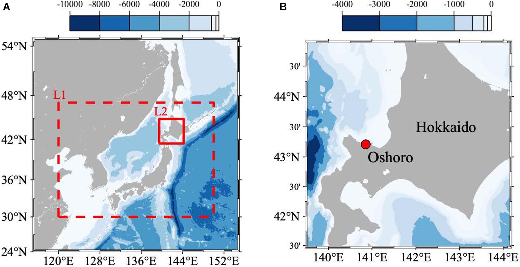
Figure 1. (A) Model domains and bathymetry (color: m) of the double-nested Regional Ocean Modeling System (ROMS). The domains of the 1/3- (L1) and 1/15- (L2) degree models are surrounded by the dashed and solid red squares, respectively. (B) The location of the study site (140°51’30”E and 43°12’34”N) is indicated by the dotted red circle in the zoomed-in region of the ROMS-L2 domain.

Monitoring

Since March 30, 2017, we have measured continuously temperature and salinity as physical parameters, and DO and pH (total scale) as biogeochemical parameters. A conductivity and temperature sensor (INFINITY-CTW ACTW-USB; JFE Advantech) was used to measure temperature and salinity hourly, while DO was measured hourly with a RINKO W AROW-USB (JFE Advantech). The accuracy of temperature, conductivity and DO is ±0.01°C, ±0.01 mS cm^–1, and non-linearity ± 2% FS (at 1 atm, 25°C), respectively. The range of the DO sensor was 0–20 mg l^–1 DO concentration (or 0–200% DO saturation) and data beyond this range were eliminated. Calibration of the DO sensor was carried out by two-point (zero and span) calibration using 0 and 100% (saturated) oxygen waters. The two sensors have mechanical wipers that periodically sweep the sensing surface to keep the initial accuracy, avoiding bio-fouling without chemical materials and frequent maintenances.

To measure pH hourly, glass electrode pH sensors (SP-11 and SPS-14; Kimoto Electric) were used. The reproducibility of pH sensors is ±0.001. The sensors were calibrated against two seawater scale pH standard buffer solutions, 2-amino-2-hydroxymethyl-1, 3-propanediol (TRIS) and 2-aminopyridine (AMP). The sensors were withdrawn for maintenance and calibration at 1- to 3-month intervals to minimize measurement biases caused by bio-fouling and measurement drift. At each calibration, it was confirmed that the sensor kept its Nernst response (ca. 0.05916V/pH at 25°C and 35.0 salinity) within the range of ±0.5%.

Seawater samples were collected when the sensors were calibrated and analyzed using a total alkalinity (TA) titration analyzer (ATT-05; Kimoto Electric) to obtain the TA and a coulometer (MODEL 3000A; Nippon ANS) to determine the dissolved inorganic carbon (DIC) concentration (Wakita et al., 2017, 2021; Yamaka, 2019). The values were calibrated against certified reference material (CRM) provided by Prof. A. G. Dickson (Scripps Institution of Oceanography, University of California San Diego) and KANSO. The precision of the analyses of both the DIC and TA was smaller than ±2 μmol kg^–1 based on replicate samples. Then, the pH (total scale) at the in situ temperature were calculated from the carbonate dissociation constants in Lueker et al. (2000) and temperature, salinity, TA, and DIC using CO2SYS (Pierrot et al., 2006). pH at time t [pH(t)] obtained by the sensor was then corrected its drift by the following equation:

$$\text{pH}\left(t\right)={\text{pH}}_m\left(t\right)+\left({\text{pH}}_{\text{sample}}(t_e)-{\text{pH}}_m(t_e)\right)\times \frac{t-t_i}{t_e-t_i},(1)$$

where pH_m(t) represents measured value of pH by the sensor at the time t, pH_sample(t_e) and pH_m(t_e) is the pH at the end time of each deployment (t_e) obtained by the seawater sample and sensor, respectively, and t_i is the start time of each deployment.

Equation (1) assumes that drift of the pH sensor increases linearly with time over the whole period of single deployment. However, actual time course of sensor drift is not linear, so this may cause significant error in the pH(t) value after the drift correction. In 2020, we made a 55-days deployment of the same pH sensor (SP-11) that we deployed in this study into the Miyako Bay, a bay in northern Japan having similar feature with that of the Oshoro Bay. At this time, we calculated pH(t) using the same Eq. (1) but with pH_sample data obtained by weekly basis [pH₁(t)] and those obtained by bi-monthly basis [at the initial and end time of the deployment; pH₂(t)], and compared the drift-corrected values (Figure 2). We found that the root mean square of difference between pH₁(t) and pH₂(t) over the whole deployment period was 0.015. We interpreted this value as the measure of the uncertainty of pH(t) originated from different frequency of the drift correction (10 days and 2 months in this case). Therefore, we evaluate that the uncertainty of pH(t) calculated in this study is in the same order and is small enough for monitoring in the coastal regions with relatively larger daily and seasonal variations.

FIGURE 2

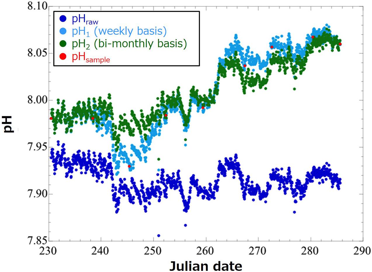
Figure 2. Time-series of pH values in the Miyako Bay in August through October 2020. Dots in blue denote raw pH values obtained by a pH sensor (SP-11; pH_raw). Those in red demote pH values calculated by referring to pH values of water samples (pH_sample). Those in light blue and green show pH values after calibration and bias correction by pH values obtained by water samples weekly (pH₁; in light blue) and bi-monthly (at the initial and end time of the deployment; pH₂; in green).

Ω_arag of the seawater samples were calculated from the carbonate dissociation constants in Lueker et al. (2000) and temperature, salinity, TA, and DIC using CO2SYS (Pierrot et al., 2006). Ω_arag was also estimated using CO2SYS, with TA, the monitored temperature, and salinity. As no continuous monitoring TA data exist, we used the TA value obtained with a regression equation for north of 30°N in the North Pacific (Lee et al., 2006):

$$\text{TA}(\mathrm{\mu }\text{m}\text{o}\text{l}\text{k}{\text{g}}^{-1})=\mathrm{\hspace{0.33em}2305}+53.23\left(\text{salinity}-35\right)+1.85$$

$${\left(\text{salinity}-35\right)}^2-14.72(\text{temperature}({}^{\circ }\mathrm{C})-20)$$

$$-0.158{(\text{temperature}({}^{\circ }\mathrm{C})-20)}^2+0.062$$

$$\mathrm{\hspace{1em}}\mathit{\hspace{1em}}(\text{temperature}({}^{\circ }\mathrm{C})-20)\times \text{longitude}({}^{\circ }),(2)$$

where the longitude of the study site is 140.86°E (Figure 1B).

Modeling

The current and future states of physical and biogeochemical parameters were simulated using the Regional Ocean Modeling System (ROMS). Of the versions of ROMS, we chose ROMS-Agrif (Penven et al., 2006), which embeds an ecosystem model (Pelagic Interactions Scheme for Carbon and Ecosystem Studies (PISCES); Aumont et al., 2003) in the ROMS. The bathymetry was expressed using the Earth 1 Arc Minute Topography Model (ETOPO1; Amante and Eakins, 2009).

The ROMS was downscaled (nested) twice (Figure 1A; Yamaka, 2019; Akamatsu, 2020). The first ROMS (L1) had a horizontal resolution of 1/3 degree and a temporal resolution of 1 h. To simulate physical and biogeochemical parameters using L1, boundary and initial conditions were needed. For this simulation, the Comprehensive Ocean-Atmosphere Data Set (COADS) 2005 (Da Silva et al., 1994) was used for the atmospheric forcing. For the oceanic physical and biogeochemical forcing, the World Ocean Atlas (WOA) 2009 (Goyet et al., 2000; Aumont and Bopp, 2006; Antonov et al., 2010; Garcia et al., 2010; Locarnini et al., 2010) was used. For future projection, the climate model outputs of the MIROC-EMS (model description and basic results of CMIP5-20c3m; Watanabe et al., 2011). Representative Concentration Pathways (RCP) 2.6 and 8.5 scenarios were used. The outputs of L1 were used as boundary and initial conditions to drive a second ROMS (L2) with a horizontal resolution of 1/15 degree and a temporal resolution of 1 h. The model was spun up for 5 years by driving with the 10-year mean current (1996–2005) and future (2086–2095) boundary conditions and the model outputs for the last 5 years were averaged and analyzed in this study.

When the monthly-averaged model results were compared with the corresponding observed results, the model results still differed from the observed results and the extent of model-observation misfits differs largely among parameters and months (Figure 3). One of the possible reasons for the model-observation misfits is because the spatial resolution of L2 is still a bit too coarse to simulate the Oshoro bay. The other possible reason is because the model does not embed local processes such as inputs of freshwater and terrestrial nutrients to the coast, and primary production by seagrass/seaweeds. For example, as explained in 3.1, substantially low salinity was observed from late winter to early spring (in March and April), which was caused by the inflow of snow-melt water discharged directly to the bay from the surrounding land (Nakata et al., 2001). Such observed processes were not able to be reproduced by the model. Also, as well as phytoplankton bloom, abrupt primary production by seagrass/seaweeds is dominant in spring (in April through June) in the study site, which is not reproduced explicitly by the ecosystem model used in this study in which phytoplankton are assumed to be primary producers. This might lead to relative underestimation of modeled DO in spring even though the modeled temperature is underestimated, too. In this study, the biases between the observed and modeled results were corrected using a procedure adapted by Yara et al. (2011). Hence,

FIGURE 3

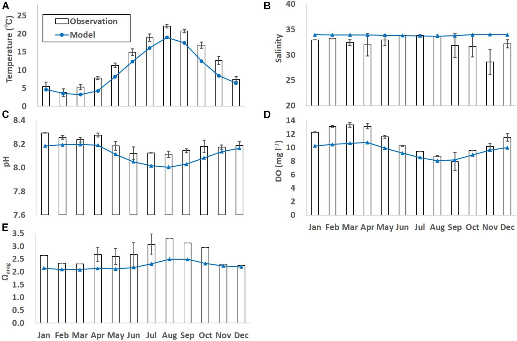
Figure 3. Monthly-mean observed and modeled (A) temperature (°C), (B) salinity, (C) dissolved oxygen (DO; mg l^{– 1}), (D) pH, and (E) Ω_arag. The error bars denote one standard deviation of the observed results. Black bars and blue lines denote observed and model results for the current states, respectively.

$${\mathrm{\Phi }}_f={\mathrm{\Phi }}_{\text{obs}}+\mathrm{\Delta }\mathrm{\Phi },(3)$$

$$\mathrm{\Delta }\mathrm{\Phi }={\mathrm{\Phi }}_f-{\mathrm{\Phi }}_p,(4)$$

where Φ_f is the future modeled value of a parameter, and Φ_obs and Φ_p are the present observed and modeled values of the parameter, respectively.

Results

Physical Parameters

Large seasonal fluctuation in the water temperature was found (Figure 4A). The maximum and minimum temperatures during the monitoring period were 24.3°C in August 2018 and 0.9°C in February 2019, respectively. These were similar to observations at three sites at depths of 0 and 5 m in the same bay in the 1990s (Nakata et al., 2001).

FIGURE 4

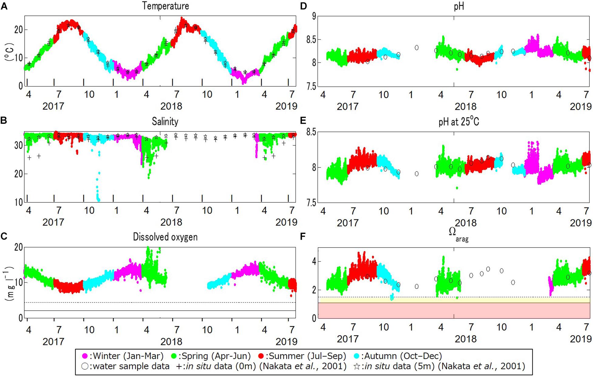
Figure 4. Time series monitoring data for (A) temperature (°C), (B) salinity, (C) dissolved oxygen (DO; mg l^–1), (D) pH, (E) pH standardized at 25°C (pH_25°C), and (F) the aragonite saturation state (Ω_arag) at the study site, in boreal winter (January through March; in magenta), spring (April through June; in green), summer (July through September; in red), and autumn (October through December; in light blue), from March 30, 2017, to July 22, 2019. Crosses and stars in (A,B) denote the observational data at 0 and 5 m depths at the study site obtained in a previous study (Nakata et al., 2001). Open dots in (D–F) denote in-situ values obtained by water samples. The dotted and solid lines in (C) denote the critical level for deoxygenation in Turner et al. (2005) and Vaquer-Sunyer and Duarte (2008; 2.0 mg l^–1), and Marumo and Yokota (2012; 4.29 mg l^–1), respectively. Yellow and red domains in (f) denote the marginal and critical level of ocean acidification for calcifiers compiled in previous studies (between 1.1 and 1.5 and below 1.1 for Ω_arag, respectively; e.g., Waldbusser et al., 2015; Onitsuka et al., 2018).

The salinity also fluctuated seasonally, but in a more complicated manner (Figure 4B). The maximum and minimum salinity during the monitoring period was 35.9 in July 2017 and 10.8 in November 2017, respectively. The salinity was relatively low from late winter to early spring as a result of the inflow of snow-melt water discharged directly to the bay from the surrounding land, as also mentioned in Nakata et al. (2001). The low salinity that appeared sporadically in November 2017 was first found by the continuous monitoring. This sudden low salinity was thought to be associated with an extreme storm on November 11, 2017.

Biogeochemical Parameters

The DO also showed strong seasonal fluctuation, and was generally high in boreal winter (January – March) and low in boreal summer (July – September; Figure 4C). The maximum and minimum DO during the monitoring period was 19.8 mg l^–1 in April 2018 and 7.2 mg l^–1 in August 2017, respectively. The seasonal fluctuation was characterized by the difference in oxygen saturation with temperature, and was high in cold water and low in warm water. The DO concentration is negatively correlated with temperature year-round, with a strong annual mean negative correlation of R = –0.86 (Table 1 and Figure 5A).

TABLE 1

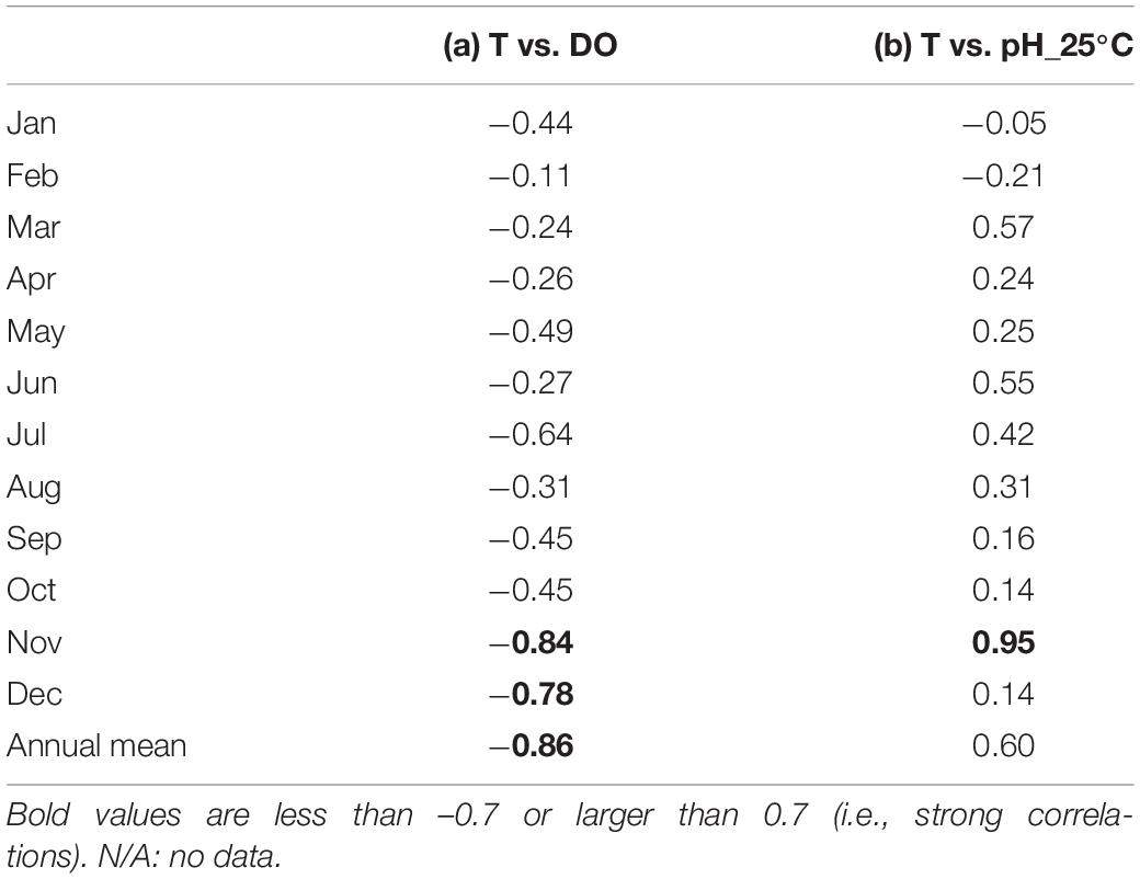
Table 1. Monthly- and annual-mean observed correlation coefficients between (a) temperature (T) and dissolved oxygen (DO),and (b) temperature and pH standardized at 25°C (pH_25°C) at the study site.

FIGURE 5

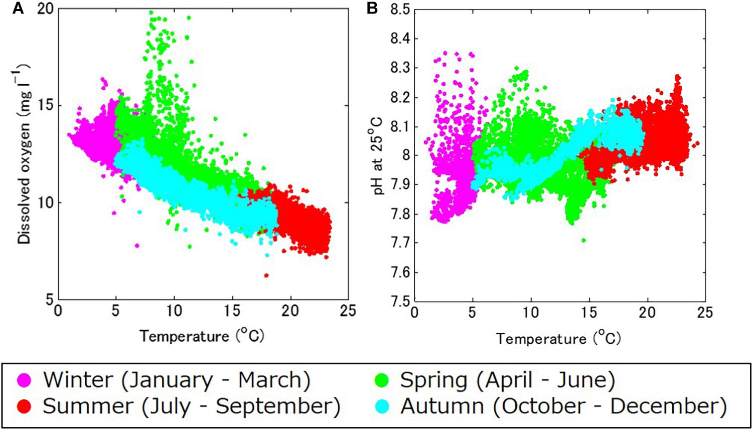
Figure 5. (A) Temperature–dissolved oxygen (DO), and (B) temperature–pH standardized at 25°C (pH_25°C) diagrams for the study site, in winter (January through March; in magenta), spring (April through June; in green), summer (July through September; in red), and autumn (October through December; in light blue).

The DO also showed clear daily fluctuation, unlike the physical parameters. A maximum amplitude of 9.5 mg l^–1 was recorded in May 2018 during the spring bloom (Figure 4C; Yamaka, 2019). The maximum amplitude was comparable to or larger than reported in other coastal regions (e.g., 220 μmol kg^–1 or around 6.9 mg l^–1; Frieder et al., 2012). DO is generally higher in the daytime and lower at night (Figure 6A). The daily fluctuation in DO concentration is consistent with DO produced by photosynthesis by primary producers, such as phytoplankton, seaweeds, and seagrasses in the daytime and DO consumption by the respiration of all marine organisms at night. Therefore, the daily amplitude of DO concentration was relatively large in boreal spring (April - June) when photosynthesis was active, and the monthly-mean value was the largest in April (1.6 mg l^–1; Figure 7A).

FIGURE 6

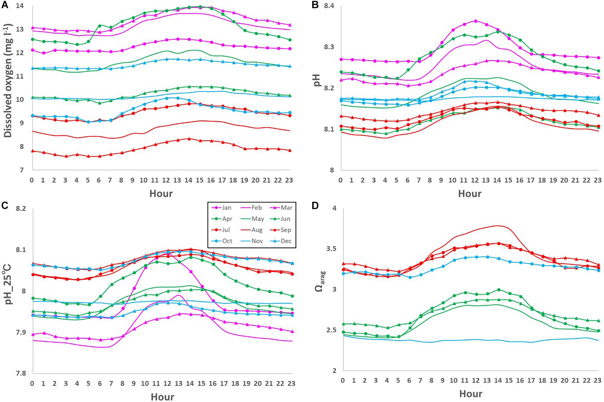
Figure 6. Monthly-mean daily fluctuations in (A) dissolved oxygen (DO; mg l^{– 1}), (B) pH, (C) pH_25°C, and (D) Ω_arag from 0 am to 11 pm.

FIGURE 7

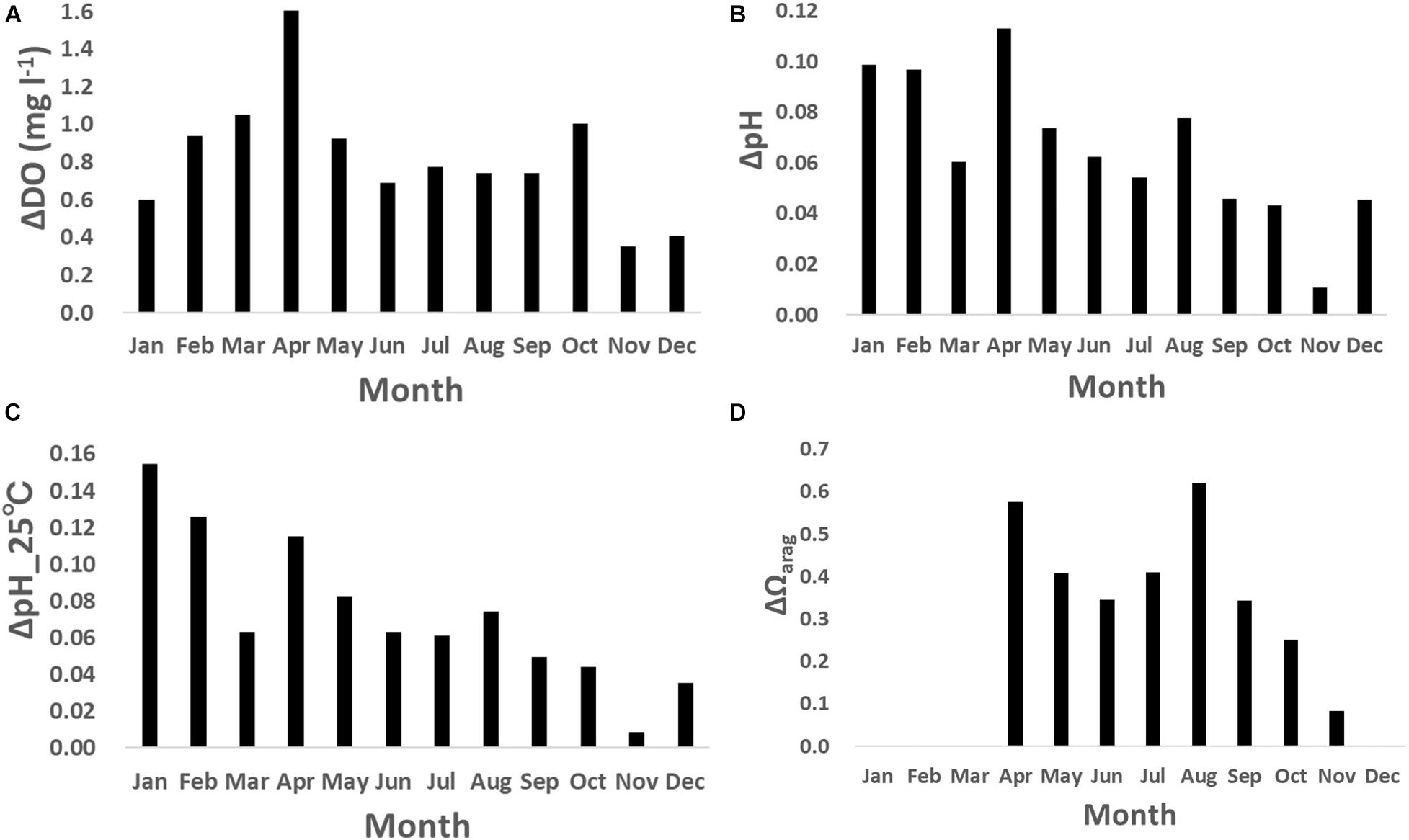
Figure 7. Monthly-mean daily amplitude of (A) dissolved oxygen (DO; mg l^{– 1}), (B) pH, (C) pH_25°C, and (D) Ω_arag.

Accordingly, pH showed similar seasonal and daily fluctuations (Figures 4D,E, 6B,C). The maximum and minimum pH during the monitoring period was 8.72 (pH_25°C = 8.35) in February 2019 and 7.86 (pH_25°C = 7.71) in June 2018, respectively. Similar to DO, the seasonal and daily fluctuations were primarily characterized by physical and biogeochemical processes, respectively. The pH is dependent on temperature and is high in cold water and low in warm water, which contributes to the seasonal fluctuation in pH. The monitored pH_25°C had a positive correlation with the temperature (an annual-mean correlation coefficient of R = 0.60; Table 1 and Figure 5B), although the correlation varied seasonally.

Similar to the DO concentration, there was a daily fluctuation in pH, which was high in the daytime and low at night, due to photosynthesis by primary producers in the daytime and respiration by marine organisms at night (Figures 6B,C). The daily amplitude was relatively large in April, when photosynthesis is predominant, and the monthly-mean was the largest in April (0.11; Figure 7B), similar to that of the DO concentration. The pH also fluctuated sporadically. The maximum diurnal fluctuation in the study period was 0.64 (0.42 for pH_25°C), which occurred in January 2019 (Figures 6C, 7C), and was comparable to fluctuations in estuarine (0.99), near-shore (0.49), and kelp forest (0.36-0.54) sites in other coastal regions (Hofmann et al., 2011; Frieder et al., 2012). These results indicate that coastal marine species in Oshoro Bay temporarily experienced low pH resulting from the wide diurnal variation in pH, similar to other coastal regions.

The Ω_arag, another ocean acidification metric, also showed significant seasonal and daily fluctuations, but in a more complicated way (Figure 4F). The maximum and minimum Ω_arag was 4.7 in August 2017 and 1.3 in November 2017, respectively. The extremely low Ω_arag in November 2017 is thought to be associated with an extreme storm on November 11, 2017, which caused low temperature and salinity. The sporadic lowering of Ω_arag, which is close to the critical level of ocean acidification (Ω_arag = 1.1; Onitsuka et al., 2018) was first found by multi-year monitoring. No Ω_arag values were available when either the salinity or pH data were not obtained. Therefore, it is likely that we failed to capture the annual minimum value of Ω_arag in this study. However, referring to observed seasonal fluctuations in Ω_arag (e.g., Ishii et al., 2011; Wakita et al., 2017, 2021), the annual minimum should appear in winter when the water temperature is low and the value may have already reached close to the critical level of acidification.

Similar to the DO concentration and pH, the daily fluctuation in Ω_arag was also prominent and it was high in the daytime and low at night, driven by daily fluctuation of carbon and oxygen dynamics through photosynthesis by primary producers in the daytime and respiration by marine organisms at night (Figure 6D). Although we did not cover the overall temporal fluctuation of Ω_arag because of missing data necessary for calculating the value (Figure 4F), the observed maximum daily fluctuation during the study period was 2.3 in April 2018, when the spring bloom was dominant. The monthly-mean daily amplitude was as large as 0.6 in spring and summer (Figure 7D).

Future Projections

The annual-mean projected rise in water temperature from the present to the end of this century was 2.2°C for the RCP 2.6 scenario and 5.5°C for the RCP 8.5 scenario (Figure 8A). The rise in temperature was followed by significant lowering of the DO concentration, pH, and Ω_arag in the future (Figures 8B–D). However, the extent differed between the RCP scenarios: compared to their present states both physical and biogeochemical parameters are anticipated to change significantly for RCP 8.5, but much more moderately for RCP 2.6. The estimated extent of the projected results for RCP 2.6 is closer to the present values than those for RCP 8.5, which concurred with other future projections (e.g., Takao et al., 2015).

FIGURE 8

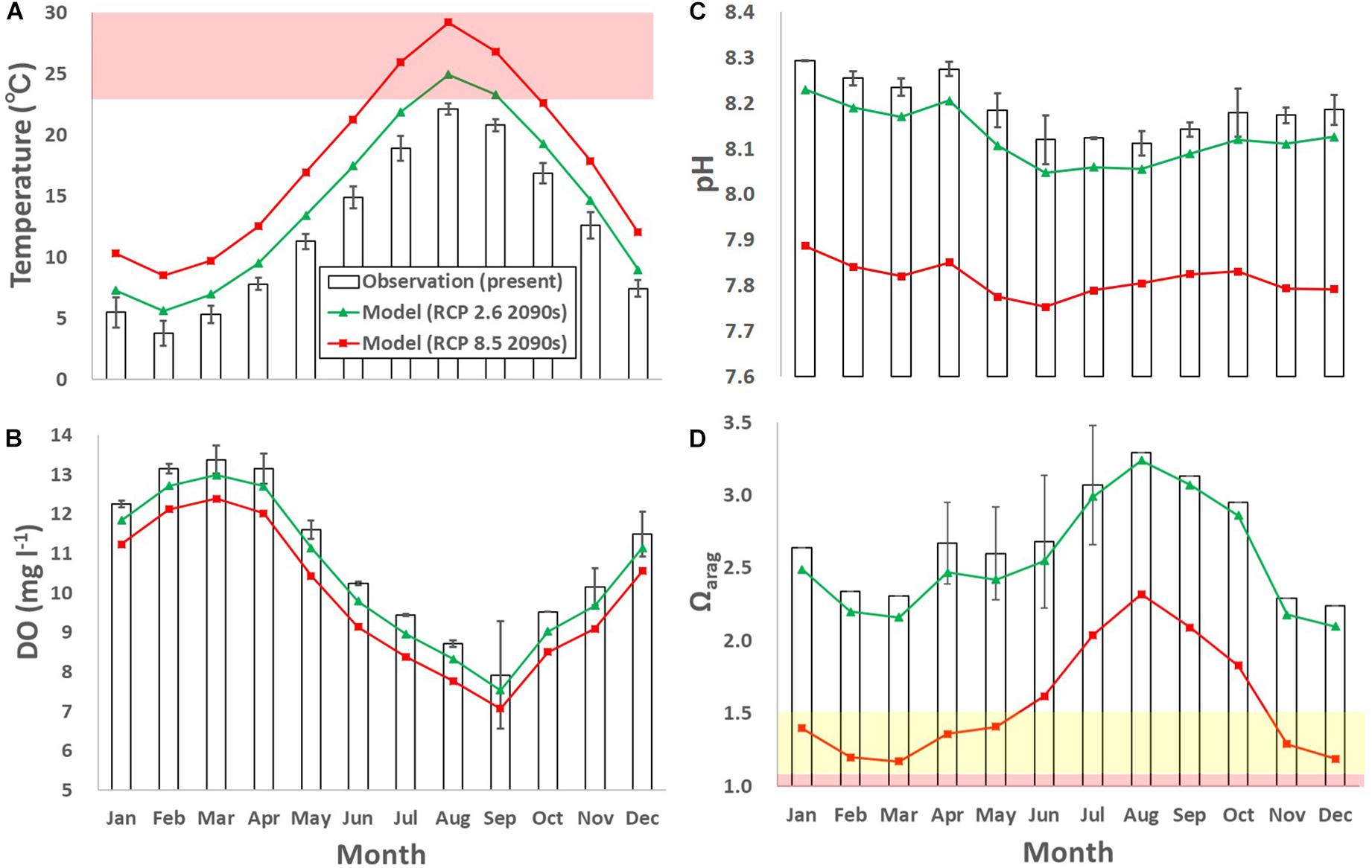
Figure 8. Monthly-mean observed and modeled (A) temperature (°C), (B) dissolved oxygen (DO; mg l^{– 1}), (C) pH, and (D) Ω_arag. The error bars denote one standard deviation of the observed results. Green and red lines denote model results for the 2090s with the RCP 2.6 and 8.5 scenarios, respectively. The red domain in (A) denotes the critical level of ocean warming for sea urchins and scallops (over 23°C; Hoshikawa, 2006; Shibano et al., 2014), both of which are main fisheries targets of the subarctic coast. Yellow and red domains in (D) denote the marginal and critical level of ocean acidification for calcifiers compiled in previous studies (between 1.1 and 1.5 and below 1.1 for Ω_arag, respectively; e.g., Waldbusser et al., 2015; Onitsuka et al., 2018).

The projected annual-mean DO concentration decreased by 0.43 mg l^–1 for RCP 2.6 and 1.02 mg l^–1 for RCP 8.5, from the present (Figure 8B). Similarly, the projected annual-mean pH decreased by 0.06 for RCP 2.6 and 0.38 for RCP 8.5, from the present (Figure 8C). The projected pH reduction for RCP 2.6 and RCP 8.5 is comparable to that projected globally in previous studies (0.06–0.07 and 0.30–0.33, respectively; e.g., IPCC AR5, Jiang et al., 2019). The projected annual-mean Ω_arag decreased by 0.1 for RCP, 2.6 and 1.1 for RCP 8.5, from the present (Figure 8D).

Discussion

Criteria for Ocean Warming, Acidification, and Deoxygenation

Several studies have reported marginal levels for calcifiers for ocean acidification of Ω_arag = ca. 1.1–1.5 [e.g., Waldbusser et al., 2015 for bivalve larvae, Zhan et al., 2016 for sea urchin (S. intermedius), and Onitsuka et al., 2018 for Ezo abalone larvae]. The marine environment is suitable for calcifiers above the marginal levels and unsuitable (critical) below them, while the levels differ with species abundance, life stages and locations.

The monitoring showed that the Ω_arag did not reach the critical level in the study period, but was sometimes marginal (Figure 4F). For the RCP 8.5 scenario, the monthly-mean Ω_arag is very often marginal in the 2090s. Considering that the future daily fluctuations of the biogeochemical parameters presumably magnify as the buffer capacity weakens, the daily minimum values will more often reach critical levels for calcifiers (<1.1 for Ω_arg). Previous experimental results showed that the growth and malformation rates of larval Ezo abalone decreased and increased greatly, respectively, when the larvae were exposed in experimental seawater in which the Ω_arag was about 1.1, even for only 2–3 days (Onitsuka et al., 2018). This implies that more frequent future critical levels may severely damage calcifiers, especially during their early stages when they are relatively vulnerable to high CO₂. This will also affect local industries, especially shellfisheries. Because around 60% of the shellfish and half of the calcifiers in Japan are caught in subarctic seas in which the Ω_arag is relatively low, ocean acidification is of great concern and the social demand for adaptive fisheries, such as changing the aquaculture style as mentioned in section “Suggestion for future adaptation,” in response to global change is high.

Similarly, several studies have reported various critical levels for deoxygenation in which the DO concentration is <2.0 mg l^–1 (Turner et al., 2005; Vaquer-Sunyer and Duarte, 2008) or 4.29 mg l^–1 (Marumo and Yokota, 2012). Our monitoring results show that the minimum DO concentration during the study period (7.2 mg l^–1 in August 2017) was still above the critical level (Figure 4C). However, similar to pH and Ω_arag, if we assume that the daily fluctuation in DO concentration in the future is similar to that at present, i.e., the maximum daily fluctuation is as large as 9.5 mg l^–1, the daily minimum DO concentration might often reach critical levels of less than 2.0 mg l^–1 in the future.

Along with ocean acidification and deoxygenation, concurrent ocean warming may also affect marine organisms, including calcifiers. For example, the main fisheries targets in the study site are vulnerable to warm temperatures. A representative critical temperature level was reported to be 23°C for sea urchins and scallops (Hoshikawa, 2006; Shibano et al., 2014). Temperatures over 23°C are not common at the study site now, but are projected to appear for 2 months for the RCP 2.6 scenario and 3 months for the RCP 8.5 scenario in summer (Figure 8A). This means that calcifiers along the subarctic coast will suffer from ocean acidification in winter and ocean warming in summer in the future.

Suggestion for Future Adaptation

The large difference in the future projections between the RCP 2.6 and 8.5 scenarios clearly shows the need to reduce anthropogenic CO₂ and other greenhouse gas emissions as per the Paris Agreement, which has a target similar to the RCP 2.6 pathway, to alleviate fatal impacts of global change on marine organisms along subarctic coasts. It is also important to adapt to the upcoming impacts of global change. Adaptation strategies include modifying local industries in subarctic coastal regions, such as fisheries, and tourism such as eating around seafoods and recreational scuba diving. Because of overused fisheries resources, aquaculture plays a greater role in maintaining a steady supply of fisheries resources. Shellfish such as scallops, oysters, and abalone, and sea urchins are all calcifiers, and therefore, are concerned to be more or less affected by ocean acidification. However, the vulnerability to low pH and Ω_arag differs with various aspects such as the species abundance, life stage and habitats. For example, possible adaptation strategies to upcoming ocean acidification include changing the aquaculture style, such as raising larval calcifiers in low CO₂ conditions manipulated artificially, such as on-land aquaculture (e.g., Fujii, 2020), following the scientific insights that early larvae are relatively vulnerable to high CO₂ (e.g., Kurihara, 2008; Kimura et al., 2011; Waldbusser et al., 2015; Onitsuka et al., 2018; Foo et al., 2020). Combined impacts of global warming and ocean acidification are generally concerned to magnify the adverse effects on calcifiers, while global warming may partly and temporally alleviate the impacts of ocean acidification by rise in alkalinity from the land, as already evidenced in some other subarctic regions (e.g., Watanabe et al., 2009; Salisbury and Jönsson, 2018).

Regarding deoxygenation, low oxygen conditions are due to local human impacts, as well as global change and subsequent ocean warming. As local human impacts such as nutrification from the land are easier to alleviate than global change, further regulation of nutrient discharge to the coasts should delay the serious impacts of deoxygenation on marine organisms (e.g., Rabalais et al., 2010). However, the extent of regulation of nutrient discharge has not yet been quantified and further analytical studies are required.

Conclusion

This study was the first multi-year in-situ monitoring study of a subarctic coast and produced future projections of physical and biogeochemical parameters related to global change-driven ocean warming, acidification, and deoxygenation. The monitoring identified new characteristics of physical and biogeochemical parameters at the study site, such as sporadic changes in salinity and DO, which revealed that marine creatures sometimes experience marginal levels of ocean acidification. Our future projection results suggest that in the future high CO₂ world, calcifiers that are accustomed to current subarctic environments may be seriously damaged by ocean warming in summer and ocean acidification in mid-winter, and possibly by deoxygenation assuming that the daily fluctuation in DO concentration in the future is similar to that at present. Therefore, the mitigation of global change by following the Paris Agreement is of great importance for saving marine ecosystems and local industries, although local adaptation strategies are also required, such as adjusting aquaculture styles.

Data Availability Statement

The raw data supporting the conclusions of this article will be made available by the authors, without undue reservation.

Author Contributions

MF, ST, TY, TA, YF, MW, AY, and TO contributed to the study conception and design. All authors contributed to the manuscript revision and have read and approved the submitted version.

Funding

This study was supported by the Integrated Research Program for Advancing Climate Models (TOUGOU) Grant Numbers JPMXD0717935498 and JPMXD0717935715 from the Ministry of Education, Culture, Sports, Science, and Technology (MEXT), Japan, the Japan Society for the Promotion of Science (JSPS) KAKENHI Grant Number JP 15H04536, 16H01792, and 20H04349, Study of Biological Effects of Acidification and Hypoxia (BEACH) of the Environment Research and Technology Development Fund Grant Number JPMEERF20202007 of the Environmental Restoration and Conservation Agency of Japan, and Hokkaido University Functional Enhancement Project.

Conflict of Interest

The authors declare that the research was conducted in the absence of any commercial or financial relationships that could be construed as a potential conflict of interest.

Acknowledgments

We thank Hisashi Endo, Haruko Kurihara, Koji Suzuki, Michiyo Yamamoto-Kawai, and Takeshi Yoshimura for their fruitful discussion and helps on monitoring and water sample analyses. We also thank Norishige Yotsukura, Koji Shibazaki, and Norifumi Sugimoto of the Oshoro Marine Station, Hokkaido University, and Wakako Takeya and Serina Maehara for their support with the monitoring, and Hiroyoshi Sumita of Kaiyoutansa for his suggestion regarding monitoring and installation. Thanks are also extended to Richard Feely and two reviewers for their practical and useful comments.

References

Akamatsu, T. (2020). Projecting the Impacts of Climate Change On Coral Distribution In The Temperate Area Of Japan. Master’s thesis. Graduate School of Environmental Science, Hokkaido University, 66.

Google Scholar

Amante, C., and Eakins, B. W. (2009). “ETOPO1 1 Arc-minute global relief model: procedures, data sources and analysis,” in NOAA Technical Memorandum NESDIS, NGDC 24, (Washington, DC: NOAA), 19.

Google Scholar

Antonov, J. I., Seidov, D., Boyer, T. P., Locarnini, R. A., Mishonov, A. V., Garcia, H. E., et al. (2010). WORLD OCEAN ATLAS 2009, Volume 2: Salinity. NOAA Atlas NESDIS 69. Washington, DC: NOAA, 184.

Google Scholar

Aumont, O., and Bopp, L. (2006). Globalizing results from ocean in situ iron fertilization studies. Global Biogeochem. Cycles 20:GB2017.

Google Scholar

Aumont, O., Maier-Reimer, E., Blain, S., and Monfray, P. (2003). An ecosystem model of the global ocean including Fe, Si, P colimitations. Global Biogeochem. Cycles 17:GB1060.

Google Scholar

Barton, A., Hales, B., Waldbusser, G. G., Langdon, C., and Feely, R. A. (2012). The Pacific oyster, Crassostrea gigas, shows negative correlation to naturally elevated carbon dioxide levels: Implications for near-term ocean acidification effects. Limnol. Oceanogr. 57, 698–710. doi: 10.4319/lo.2012.57.3.0698

CrossRef Full Text | Google Scholar

Baumann, H., Wallace, R. B., Tagliaferri, T., and Gobler, C. J. (2014). Large natural pH, CO₂ and O₂ fluctuations in a temperate tidal salt marsh on diel, seasonal, and interannual time series. Estuaries Coast. 38, 220–231. doi: 10.1007/s12237-014-9800-y

CrossRef Full Text | Google Scholar

Bednaršek, N., Feely, R. A., Beck, M. W., Alin, S. R., Siedlecki, S. A., Calosi, P., et al. (2020). Exoskeleton dissolution with mechanoreceptor damage in larval Dungeness crab related to severity of present-day ocean acidification vertical gradients. Sci. Total Environ. 716:136610. doi: 10.1016/j.scitotenv.2020.136610

PubMed Abstract | CrossRef Full Text | Google Scholar

Christian, J., and Ono, T. (Eds) (2019). Ocean acidification and deoxygenation in the North Pacific Ocean. PICES Spec. Publ. 6:101.

Google Scholar

Da Silva, A. M., Young, C. C., and Levitus, S. (1994). Atlas of Surface Marine Data 1994, Vol. 1, Algorithms and Procedures, NOAA Atlas NESDIS 6. Washington, DC: NOAA, 74.

Google Scholar

Dai, M., Lu, Z., Zhai, W., Chen, B., Cao, Z., Zhou, K., et al. (2009). Diurnal variations of surface seawater pCO₂ in contrasting coastal environments. Limnol. Oceanogr. 54, 735–745. doi: 10.4319/lo.2009.54.3.0735

CrossRef Full Text | Google Scholar

DePasquale, E., Baumann, H., and Gobler, C. J. (2015). Vulnerability of early life stage Northwest Atlantic forage fish to ocean acidification and low oxygen. Mar. Ecol. Prog. Ser. 523, 145–156. doi: 10.3354/meps11142

CrossRef Full Text | Google Scholar

Dixson, D. L., Jennings, A. R., Atema, J., and Munday, P. L. (2015). Odor tracking in sharks is reduced under future ocean acidification conditions. Glob. Chang. Biol. 21, 1454–1462. doi: 10.1111/gcb.12678

PubMed Abstract | CrossRef Full Text | Google Scholar

Feely, R. A., Sabine, C. L., Hernandez-Ayon, J. M., Ianson, D., and Hales, B. (2008). Evidence for upwelling of corrosive “acidified” water onto the continental shelf. Science 320, 1490–1492. doi: 10.1126/science.1155676

PubMed Abstract | CrossRef Full Text | Google Scholar

Foo, S. A., Koweek, D. A., Munari, M., Gambi, M. C., Byrne, M., and Caldeira, K. (2020). Responses of sea urchin larvae to field and laboratory acidification. Sci. Total Environ. 723:138003. doi: 10.1016/j.scitotenv.2020.138003

PubMed Abstract | CrossRef Full Text | Google Scholar

Frieder, C. A., Nam, S. H., Martz, T. R., and Levin, L. A. (2012). High temporal and spatial variability of dissolved oxygen and pH in a nearshore California kelp forest. Biogeosciences 9, 3917–3930. doi: 10.5194/bg-9-3917-2012

CrossRef Full Text | Google Scholar

Fujii, M. (2020). Effects of ocean warming and acidification on marine ecosystem and societies in Japanese coasts. Fish. Eng. 56, 191–195.

Google Scholar

Garcia, H. E., Locarnini, R. A., Boyer, T. P., and Antonov, J. I. (2010). “World Ocean Atlas 2009, Volume 3: dissolved oxygen, apparent oxygen utilization, and oxygen saturation,” in NOAA Atlas NESDIS 70, ed. S. Levitus (Washington, DC: NOAA), 344.

Google Scholar

Gobler, C. J., and Baumann, H. (2016). Hypoxia and acidification in ocean ecosystems: coupled dymanics and effects on marine life. Biol. Lett. 12:20150976. doi: 10.1098/rsbl.2015.0976

PubMed Abstract | CrossRef Full Text | Google Scholar

Goyet, C., Healy, R. J., and Ryan, J. P. (2000). Global Distribution of Total Inorganic Carbon and Total Alkalinity Below the Deepest Winter Mixed Layer Depths. ORNL/CDIAC-127 NDP-076, 40. Oak Ridge, TN: Oak Ridge National Laboratory, U.S. Department of Energy,

Google Scholar

Hofmann, G. E., Smith, J. E., Johnson, K. S., Send, U., Levin, L. A., Micheli, F., et al. (2011). High-frequency dynamics of ocean pH: a multi ecosystem comparison. PLoS One 6:e28983. doi: 10.1371/journal.pone.0028983

PubMed Abstract | CrossRef Full Text | Google Scholar

Hoshikawa, H. (2006). Change of sea water temperature and recruitment of sea urchin along the coast of the Sea of Japan in Hokkaido. Kaiyo Monthly 38, 205–209.

Google Scholar

Intergovernmental Panel on Climate Change (IPCC) (2014). Climate Change 2014: Impacts, Adaptation, and Vulnerability. Part A: Global and Sectoral Aspects. Contribution of Working Group II to the Fifth Assessment Report of the Intergovernmental Panel on Climate Change. Cambridge: Cambridge University Press, 1132.

Google Scholar

IPCC (2018). Global Warming of 1.5°C. An IPCC Special Report on the Impacts of Global Warming of 1.5°C Above Pre-Industrial Levels and Related Global Greenhouse Gas Emission Pathways, in the Context of Strengthening the Global Response to the Threat of Climate Change, Sustainable Development, and Efforts to Eradicate Poverty. Geneva: IPCC.

Google Scholar

Ishii, M., Kosugi, N., Sasano, D., Saito, S., Midorikawa, T., and Inoue, H. Y. (2011). Ocean acidification off the south coast of Japan: a result from time series observations of CO₂ parameters from 1994 to 2008. J. Geophys. Res. 116:C06022. doi: 10.1029/2010JC006831

CrossRef Full Text | Google Scholar

Jiang, L.-Q., Carter, B. R., Feely, R. A., Lauvset, S. K., and Olsen, A. (2019). Surface ocean pH and buffer capacity: past, present and future. Sci. Rep. 9:18624. doi: 10.1038/s41598-019-55039-4

PubMed Abstract | CrossRef Full Text | Google Scholar

Kimura, R., Takami, H., Ono, T., Onitsuka, T., and Nojiri, Y. (2011). Effects of elevated pCO₂ on the early development of the commercially important gastropod, Ezo abalone Haliotis discus hannai. Fish. Oceanogr. 20, 357–366. doi: 10.1111/j.1365-2419.2011.00589.x

CrossRef Full Text | Google Scholar

Kurihara, H. (2008). Effects of CO₂-driven ocean acidification on the early developmental stages of invertebrates. Mar. Ecol. Prog. Ser. 373, 275–284. doi: 10.3354/meps07802

CrossRef Full Text | Google Scholar

Lee, K., Lan, T., Tong, L. T., Millero, F. J., Sabine, C. L., Dickson, A. G., et al. (2006). Global relationships of total alkalinity with salinity and temperature in surface waters of the world’s oceans. Geophys. Res. Lett. 33:L19605. doi: 10.1029/2006GL027207

CrossRef Full Text | Google Scholar

Locarnini, R. A., Mishonov, A. V., Antonov, J. I., Boyer, T. P., Garcia, H. E., Baranova, O. K., et al. (2010). “World Ocean Atlas 2009, Volume 1: temperature,” in NOAA Atlas NESDIS 68, ed. S. Levitus (Washington, DC: NOAA), 184.

Google Scholar

Lueker, T. J., Dickson, A. G., and Keeling, C. D. (2000). Ocean pCO₂ calculated from dissolved inorganic carbon, alkalinity, and equations for K1 and K2: validation based on laboratory measurements of CO₂ in gas and seawater at equilibrium. Mar. Chem. 70, 105–119. doi: 10.1016/s0304-4203(00)00022-0

CrossRef Full Text | Google Scholar

Marumo, K., and Yokota, M. (2012). Review on the hypoxia formation and its effects on aquatic organisms. Rep. Mar. Ecol. Res. Inst. 15, 1–21.

Google Scholar

Melzner, F., Thomsen, J., Koeve, W., Oschilies, A., Gutowska, M. A., Bange, H. W., et al. (2013). Future ocean acidification will be amplified by hypoxia in coastal habitats. Mar. Biol. 160, 1875–1888. doi: 10.1007/s00227-012-1954-1

CrossRef Full Text | Google Scholar

Morita, M., Suwa, R., Iguchi, A., Nakamura, M., Shimada, K., Sakai, K., et al. (2009). Ocean acidification reduces sperm flagellar motility in broadcast spawning reef invertebrate. Zygote 18, 103–107. doi: 10.1017/s0967199409990177

PubMed Abstract | CrossRef Full Text | Google Scholar

Munday, P. L., Cheal, A. J., Dixson, D. L., Rummer, J. L., and Fabricius, K. E. (2014). Behavioral impairments in reef fishes caused by ocean acidification at CO₂ seeps. Nat. Clim. Chang. 4, 487–492. doi: 10.1038/nclimate2195

CrossRef Full Text | Google Scholar

Munday, P. L., Dixson, D. L., Donelson, J. M., Jones, G. P., Pratchett, M. S., Devitsina, G. V., et al. (2009). Ocean acidification impairs olfactory discrimination and homing ability of a marine fish. Proc. Natl. Acad. Sci. U.S.A. 106, 1848–1852. doi: 10.1073/pnas.0809996106

PubMed Abstract | CrossRef Full Text | Google Scholar

Nakata, A., Yagi, H., Miyazono, A., Yasunaga, T., Kawai, T., and Iizumi, H. (2001). Relationships between sea surface temperature and nutrient concentrations in Oshoro Bay, Hokkaido, Japan. Sci. Rep. Hokkaido Fish. Exp. Stn. 59, 31–41.

Google Scholar

Onitsuka, T., Takami, H., Muraoka, D., Matsumoto, Y., Nakatsubo, A., Kimura, R., et al. (2018). Effects of ocean acidification with pCO₂ diurnal fluctuations on survival and larval shell formation of Ezo abalone, Haliotis discus hannai. Mar. Environ. Res. 134, 28–36. doi: 10.1016/j.marenvres.2017.12.015

PubMed Abstract | CrossRef Full Text | Google Scholar

Orr, J. C., Fabry, V. J., Aumout, O., Bopp, L., Doney, S. C., Feely, R. A., et al. (2005). Anthropogenic ocean acidification over the twenty-first century and its impact on calcifying organisms. Nature 437, 681–686. doi: 10.1038/nature04095

PubMed Abstract | CrossRef Full Text | Google Scholar

Penven, P., Debreu, L., Marchesiello, P., and McWilliams, J. C. (2006). Application of the ROMS embedding procedure for the Central California Upwelling System. Ocean Model. 12, 157–187. doi: 10.1016/j.ocemod.2005.05.002

CrossRef Full Text | Google Scholar

Pierrot, D., Lewis, E., and Wallace, D. W. R. (2006). MS Excel program developed for CO₂ system calculations. ORNL/CDIAC-105a. Oak Ridge, TN: Carbon Dioxide Information Analysis Center, Oak Ridge National Laboratory, doi: 10.3334/CDIAC/otg.CO2SYS_XLS_CDIAC105a

CrossRef Full Text | Google Scholar

Rabalais, N. N., Díaz, R. J., Levin, L. A., Turner, R. E., Gilbert, D., and Zhang, J. (2010). Dynamics and distribution of natural and human-caused hypoxia. Biogeosciences 7, 585–619. doi: 10.5194/bg-7-585-2010

CrossRef Full Text | Google Scholar

Salisbury, J. E., and Jönsson, B. F. (2018). Rapid warming and salinity changes in the Gulf of Maine alter surface ocean carbonate parameters and hide ocean acidification. Biogeochemistry 141, 401–418. doi: 10.1007/s10533-018-0505-3

PubMed Abstract | CrossRef Full Text | Google Scholar

Schmidtko, S., Stramma, L., and Visbeck, M. (2017). Decline in global oceanic oxygen content during the past five decades. Nature 542, 335–339. doi: 10.1038/nature21399

PubMed Abstract | CrossRef Full Text | Google Scholar

Shibano, R., Fujii, M., Yamanaka, Y., Yamano, H., and Takao, S. (2014). Spatial and temporal dynamics of coastal sea surface temperature and catches of Japanese scallop Mizuhopecten yessoensis in Hokkaido. Bull. Jpn. Soc. Fish. Oceanogr. 78, 259–267.

Google Scholar

Takao, S., Kumagai, N. H., Yamano, H., Fujii, M., and Yamanaka, Y. (2015). Projecting the impacts of rising water temperatures on the distribution of seaweeds around Japan under multiple climate change scenarios. Ecol. Evol. 5, 213–223. doi: 10.1002/ece3.1358

PubMed Abstract | CrossRef Full Text | Google Scholar

Turner, R. E., Rabalais, N. N., Swenson, E. M., Kasprzak, M., and Romaire, T. (2005). Summer hypoxia in the northern Gulf of Mexico and its prediction from 1978 to 1995. Mar. Environ. Res. 59, 65–77. doi: 10.1016/j.marenvres.2003.09.002

PubMed Abstract | CrossRef Full Text | Google Scholar

Vaquer-Sunyer, R., and Duarte, C. M. (2008). Thresholds of hypoxia for marine biodiversity. Proc. Natl. Acad. Sci. U.S.A. 105, 15452–15457. doi: 10.1073/pnas.0803833105

PubMed Abstract | CrossRef Full Text | Google Scholar

Wakita, M., Nagano, A., Fujiki, T., and Watanabe, S. (2017). Slow acidification of the winter mixed layer in the subarctic western North Pacific. J. Geophys. Res. Oceans 122, 6923–6935. doi: 10.1002/2017jc013002

CrossRef Full Text | Google Scholar

Wakita, M., Sasaki, K., Nagano, A., Abe, H., Tanaka, T., Nagano, K., et al. (2021). Rapid reduction of pH and CaCO₃ saturation state in the Tsugaru Strait by the intensified Tsugaru Warm Current during 2012–2019. Geophys. Res. Lett. doi: 10.1029/2020GL091332

CrossRef Full Text | Google Scholar

Waldbusser, G. G., Hales, B., Langdon, C. J., Haley, B. A., Shrader, P., Brunner, E. L., et al. (2015). Ocean acidification has multiple modes of action on bivalve larvae. PLoS One 10:e0128376. doi: 10.1371/journal.pone.0128376

PubMed Abstract | CrossRef Full Text | Google Scholar

Wallace, R. B., Baumann, H., Grear, J. S., Aller, R. C., and Gobler, C. J. (2014). Coastal ocean acidification: the other eutrophication problem. Estuar. Coast. Shelf Sci. 148, 1–13. doi: 10.1016/j.ecss.2014.05.027

CrossRef Full Text | Google Scholar

Watanabe, S., Hajima, T., Sudo, K., Nagashima, T., Takemura, T., Okajima, H., et al. (2011). MIROC-ESM 2010: model description and basic results of CMIP5-20c3m experiments. Geosci. Model Dev. 4, 845–872. doi: 10.5194/gmd-4-845-2011

CrossRef Full Text | Google Scholar

Watanabe, Y. W., Nishioka, J., Shigemitsu, M., Mimura, A., and Nakatsuka, T. (2009). Influence of riverine alakalinity on carbonate species in the Okhotsk Sea. Geophys. Res. Lett. 36:L15606. doi: 10.1029/2009GL038520

CrossRef Full Text | Google Scholar

Wootton, J. T., Pfister, C. A., and Forester, J. D. (2008). Dynamic patterns and ecological impacts of declining ocean pH in a high-resolution multi-year dataset. Proc. Natl. Acad. Sci. U.S.A. 105, 18848–18853. doi: 10.1073/pnas.0810079105

PubMed Abstract | CrossRef Full Text | Google Scholar

Yamaka, T. (2019). Assessment and future projection of variational characteristics of global warming and ocean acidification proxies in Oshoro Bay, Hokkaido. Master’s thesis. Graduate School of Environmental Science, Hokkaido University, 74.

Google Scholar

Yara, Y., Oshima, K., Fujii, M., Yamano, H., Yamanaka, Y., and Okada, N. (2011). Projection and uncertainty of the poleward range expansion of coral habitats in response to sea surface temperature warming: a multiple climate model study. Galaxea 13, 11–20. doi: 10.3755/galaxea.13.11

CrossRef Full Text | Google Scholar

Zhan, Y., Hu, W., Liu, M., Duan, M., Huang, X., Chang, Y., et al. (2016). The impact of CO₂-driven ocean acidification on early development and calcification in the sea urchin Strongylocentrotus intermedius. Mar. Pollut. Bull. 112, 291–302. doi: 10.1016/j.marpolbul.2016.08.003

PubMed Abstract | CrossRef Full Text | Google Scholar