Using Global-Scale Earth System Models for Regional Fisheries Applications

Introduction

Environmental conditions can affect living marine resources (LMRs) through a number of mechanisms. Physical and chemical properties such as temperature, salinity, oxygen concentration, and pH can directly influence the vital rates of many organisms. These direct effects may manifest themselves within specific populations through increasing or decreasing growth, reproduction, and mortality (Pörtner, 2012); changes in geographic distribution as populations shift toward more favorable habitat; or shifts in the phenological timing of environmentally influenced events such as phytoplankton blooms (Karp et al., 2019). Food web interactions further complicate the potential influence of even small changes within one population (Ainsworth et al., 2011; Fay et al., 2017; Marshall et al., 2017; Masi et al., 2018).

The integration of these environmental and ecological processes has become an explicit aim of regional ecosystem-based fisheries management (EBFM) frameworks (Marshall et al., 2017; Holsman et al., 2020), and global Earth system models (ESMs) offer an enticing tool to the regional fisheries scientist to potentially quantify these many impacts of environmental change on LMRs. The representation of the biosphere within these coupled models has expanded rapidly over the past several iterations of the Intergovernmental Panel of Climate Change (IPCC) assessment reports. Most general circulation models (GCMs) that participated in the Coupled Model Intercomparison Project Phase 3 (CMIP3) (Meehl et al., 2007) coupled only physical ocean and atmosphere components and did not include any representation of ocean or land biology. By CMIP5 (Taylor et al., 2012), a dozen modeling centers included an ESM variant (i.e., a GCM that also simulates chemical and biological components of the Earth system) with some form of ocean biogeochemistry (Bopp et al., 2013). The recent simulations released under CMIP6 (Eyring et al., 2016) continue this trend, with most modeling centers further developing their biogeochemical models to quantify the impact of biogeochemical and lower-trophic-level processes on both the carbon cycle and on LMRs (Kwiatkowski et al., 2020).

However, there are several complexities involved in connecting ESM output to the regional marine ecosystem models that support LMR management. Similarly to GCMs, ESMs are designed to emphasize global scale dynamics over regional processes (Stock et al., 2011). Bias correction and/or downscaling may, therefore, be required before ESMs can sufficiently capture regional patterns of greatest relevance to LMRs, particularly in productive coastal waters (Holt et al., 2009; Brown et al., 2016; Muhling et al., 2018; Xiu et al., 2018; Echevin et al., 2020; Drenkard et al., 2021). The taxonomic diversity of phytoplankton and zooplankton in ESMs may also be insufficient to represent characteristics important to higher-order consumers, such as energy density or lipid content of various zooplankton assemblages or the relative effects of ocean acidification on different plankton communities (e.g., Rose et al., 2010; Miller et al., 2017; Gao et al., 2019). In addition, even in downscaled ESMs the spatio temporal resolution may be insufficient for linking life stage-specific, highly localized responses of higher-trophic-level LMRs to their biophysical environment (Petitgas et al., 2013; Hollowed et al., 2020). As marine ecosystem models are built to capture different aspects of these responses, they can also have different theoretical frameworks, objectives, and modeling structures, leading to difficulties in the direct comparison of projections among different models (Tittensor et al., 2018; Lotze et al., 2019). Projections from marine ecosystem models coupled to ESMs can, therefore, be widely divergent, incorporating considerable uncertainty from both model types (Lotze et al., 2019). Lastly, projections of managed resources such as fish stocks are complicated by the effects of fishing removals and management structures that interact with bottom-up drivers of stock size (Woodworth-Jefcoats et al., 2015; Barange, 2019; Lotze et al., 2019). Successfully working through these issues typically requires multidisciplinary collaborations with expertise from physical and biological oceanography up through resource assessment and management (Stock et al., 2011; Hollowed et al., 2020). Despite these challenges, ESMs offer an opportunity to provide LMR managers with projections of future ecosystem states, facilitating the development of climate-resilient management strategies.

While a number of existing studies discuss, in comprehensive detail, the predicted changes in lower trophic level variables across the suite of CMIP5 and CMIP6 ESM model simulations and the potential mechanisms underlying both the mean trends and variations between models (Bopp et al., 2013; Laufkotter et al., 2015; Kwiatkowski et al., 2020), these comparisons typically focus on large-scale patterns in nutrient cycling and are primarily targeted toward a biogeochemistry audience. For the reasons detailed above, the LMR end user typically approaches these models from a different perspective (Rose et al., 2010), and the output variables in which they are most interested may show different trends, variabilities, and skills across the spatiotemporal scales of interest (Table 1). In this study, we follow in the footsteps of these existing reviews, particularly Laufkotter et al. (2015) and Séférian et al. (2020), but from the point of view of a regional fisheries end user. The performance of each model may vary widely depending on the region of focus and the scientific question under consideration, and attempting to perform a full intercomparison of global ESM simulation output on a regional scale is well beyond the scope of this study. Instead, we highlight key structural differences within the CMIP6 suite of ESMs and discuss the ways in which these differences may lead to variability among the predicted ecological indicators most relevant for higher trophic levels. We hope that by highlighting these structural differences, we provide an entry point for LMR end users to better diagnose the potential drivers of biogeochemical and ecosystem uncertainties within their regions of interest.

TABLE 1

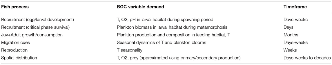
Table 1. Biogeochemical model output variables of interest for purposes of constraining fish processes.

Access to, Use of, and Interpretation of Global-Scale ESMs

While an ESM is often referred to as a single entity, each ESM is made up of many coupled sub-models representing the different components of the Earth system. Within modern ESMs, these components typically include the atmosphere, ocean, land, ocean biogeochemistry, and sea ice. While the primitive equations governing the atmospheric and ocean components of ESMs are well established, ocean biogeochemical models are less mature, often based on empirical relationships and with far fewer observations constraining the underlying equations and parameters than in their physical counterparts. As a result, the state variables and process equations included in both global and regional scale biogeochemical models vary widely, with model complexity ranging from three- to four-box nutrient/phytoplankton/zooplankton/detritus models to complex multi resource, multiple-plankton functional type models with dozens of state variables (Friedrichs et al., 2007). Even within model intercomparison experiments, there is little standardization of prognostic biogeochemical models; for example, only gas exchange and carbonate chemistry are standardized within the CMIP6 protocol, with all other processes (e.g., primary production, nutrient cycling, and plankton community composition) left to the discretion of individual modeling centers (Orr et al., 2017). Substantial differences also exist in the parameterization of unresolved physics among models (due to their computationally limited spatial/temporal resolution) with potentially strong impacts on biogeochemistry.

Table 2 includes a comprehensive list of all models that contributed at least one ocean biogeochemical output variable to the CMIP5 or CMIP6 experiments. The coupled model acronyms listed in this table correspond to the data set names used by the Earth System Grid Federation (ESGF) data portal where the model data for the CMIP experiments can be found (https://esgf-node.llnl.gov/search/cmip6/). The biogeochemical models used within this collection range from the carbonate chemistry OCMIP protocol (Orr et al., 2017), without any explicit simulation of biotic processes, to the full ecosystem models. Given time and resource constraints, using this entire suite of ESMs is impractical for a regional application. Therefore, the first step in using global ESMs in a regional context typically involves choosing the subset of ESMs best suited to answering the research question of interest. However, making an informed choice on this front can be a daunting task due to the high complexity of the numerous ESMs.

TABLE 2

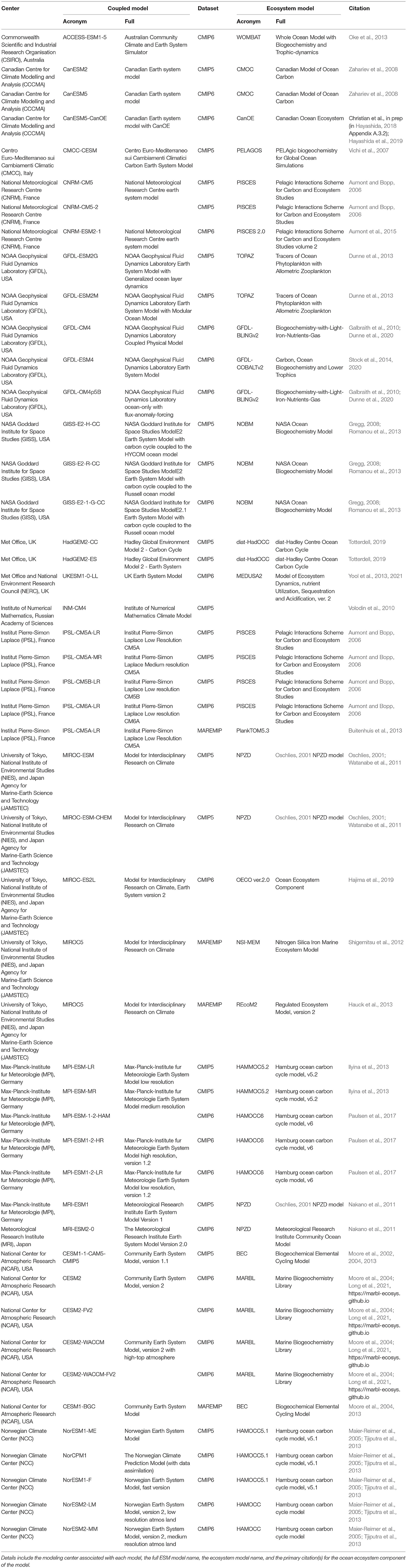
Table 2. A list of global earth system models from the 5th and 6th Coupled Model Intercomparison Projects (CMIP5 and CMIP6).

A variety of best practices have been suggested regarding choosing global ESMs to address regional questions, either through direct use or via statistical or dynamical downscaling (Drenkard et al., 2021). One suggestion is to choose models whose outputs span the envelope of uncertainty for a key variable (Cheung et al., 2016; Pozo Buil et al., 2021). Alternatively, one may limit use to models that faithfully capture the historical observed state of a particular quantity that is known to affect the ecosystem of interest, e.g., seasonal sea ice in the Bering Sea (Overland et al., 2011), upwelling and horizontal transport off the California coast (Combes et al., 2013; Di Lorenzo et al., 2013), or hypoxia due to riverine influence in the Gulf of Mexico (de Mutsert et al., 2016; Fennel et al., 2016). Between these two alternatives is a model choice based on emerging constraints (Eyring et al., 2019; Hall et al., 2019), which is a process-based approach that acknowledges that some models are likely better suited than others for a given climate change application but also that historical model fidelity does not necessarily translate to accurate climate sensitivity under future forcing (Pierce et al., 2009).

Consideration of the broad array of biogeochemical model specifications can be beneficial when using ESMs within an LMR context, both for informing the choice of which models can best address the relevant questions and interpreting the potential underlying mechanisms leading to inter-ESM differences in output. This is particularly important given the large influence of biogeochemical model structure and parameterization on an long-term predictions of LMR-relevant variables of ESM such as pH, oxygen, and net primary productivity. Within long-term climate change simulations, Frölicher et al. (2016) found that while uncertainties related to ESM internal variability and emissions scenario choice dominate the predicted end-of-century uncertainty range for physical ocean variables like temperature and carbon chemistry variables like pH, biological output variables like net primary production were far more sensitive to model uncertainty (i.e., uncertainty resulting from the use of different numerical formulations and parameterizations for physical and biological processes).

However, from a practical standpoint, making an informed choice regarding which ESMs to use for a regional application can be difficult. While global model documentation has become more common and more cohesive in recent years (Journal of Advances in Modeling Earth Systems, 2018–2020), and model cross-comparisons are available in the literature (e.g., Kwiatkowski et al., 2020; Séférian et al., 2020), this model documentation is often disconnected from common data access points and, therefore, difficult for end users unfamiliar with the biogeochemical literature to locate. Major modeling experiments (e.g., CMIP3, CMIP5, and CMIP6) do not include “release notes” to highlight how models have changed from one iteration to the next, and often the specific details of a model are spread over numerous publications, reflecting the iterative development of each model. The lack of centralized documentation or cross-comparison of the many ESM options available to LMR end users often presents a barrier to making an informed choice regarding model selection. Additionally, LMR researchers often encounter challenges in accessing model output. The storing and sharing of very large datasets is a challenge for the major modeling centers; their choices of which variables to archive and at what resolution are often driven by limited space and do not always meet LMR needs for high spatiotemporal resolution. Public datasets often include only a small subset of the depth-resolved ocean and biogeochemical variables at a monthly temporal resolution. Even monthly resolution may not be sufficiently fine to resolve phenological patterns in biologically relevant fields; for example, Asch et al. (2019) used 8-day resolution ESM output to resolve sub-monthly shifts in mean phytoplankton bloom timing under climate change. In the past, LMR scientists have needed to establish personal relationships within major modeling centers in order to get access to non-publicly archived variables. In cases where the variables of interest were not archived, either at all or at sufficient resolution, new ESM simulations may be needed, increasing the need for direct collaboration even further. This level of collaboration is difficult to maintain with even one modeling center, much less multiple; this high barrier to access further complicates the process of making an informed selection of ESMs.

In the following sections, we compare and contrast how key biogeochemical processes are represented within the CMIP6 models with explicit biogeochemical models. We choose this subset from the full list in Table 2 as a practical consideration, given that these models are most likely to be of interest to LMR end users in the coming years. We do not attempt to analyze differences in output values or how skillfully each model performs when compared to observations. Particularly when extracting results within a small region, as is typical in LMR applications, which models are most appropriate can be dependent on the exact research question being asked. For an overview of model performance across the CMIP5 and CMIP6 generations of models, we instead refer readers to Séférian et al. (2020). This study instead is intended to demystify some of the key processes being simulated within complex ESMs, allowing LMR end users to make more informed choices with regard to the models that may best suit their applications and to diagnose potential sources of model spread that influence predictions of LMR-relevant metrics.

A Comparison of CMIP6 ESMs

We focus on a few common features of the CMIP6 ESMs for this intercomparison: the structure of each model (i.e., the state variables and biological processes included), the formulations used to calculate primary production, the role of temperature in mediating various biological rates, zooplankton predator-prey function responses, detrital remineralization formulations, and river runoff implementations. These particular features were chosen as key components shared across the models that are most likely to influence the metrics, such as primary and secondary production, zooplankton biomass and community composition, and trophic transfer efficiency, that LMR end users may be most interested in. These metrics are typically those that can be used to predict species biomass, recruitment, and survival; shifts in spatial distribution; and trophic interactions, particularly with respect to target species of commercial, recreational, and subsistence harvest (Tommasi et al., 2021). The highlighted dissimilarities between models may play varying roles in contributing to inter-model spread, depending on the particular region, ecosystem, and metric of interest, but we hope that highlighting these model differences will provide a starting point for the often complex task of connecting model uncertainty to specific physical and biogeochemical drivers.

We note that there are also a few processes that may be of potential interest to LMR researchers that we chose not to highlight. We do not address processes related to gas exchange or carbonate chemistry; these processes are explicitly specified as part of the CMIP6 Ocean Model Intercomparison Project biogeochemical (OMIP-BGC) simulation protocols (Orr et al., 2017) and as such are implemented in the same way across all models within the CMIP6 suite. We also do not address certain processes that involve the coupling of the biogeochemical model components to other parts of the earth system, such as atmospheric deposition of iron. We avoid these processes primarily as a practical consideration, since they are not part of the biogeochemical models themselves, but rather a function of the other model components (such as the atmospheric and land models) that each biogeochemical model may be coupled to. We make an exception for river runoff, given its often large impact on the near-shore ecosystems that are of interest to LMR scientists.

Functional Groups and Processes

The CMIP6 models vary widely in structural complexity. This variety reflects the numerous applications for which different models were designed. Many ESMs were originally designed primarily to “close” the carbon cycle, i.e., to allow the full inventory of the oceanic processes influencing oceanic sequestration of carbon emissions. As such, their focus was less on resolving the ecosystem components themselves but rather on constraining the biologically mediated fluxes of carbon between the surface waters and deep ocean. More recently, ESMs have developed a dual role, serving both the original carbon system closure purpose and the ability to resolve energy transfer within more realistic and complex planktonic food webs. In terms of structural complexity, the CMIP6 biogeochemical models can be loosely grouped into a few categories.

At the simple end of the spectrum lies BLING, the biogeochemical model that runs within the CM4 model of GFDL (Figure 1). With only three explicitly tracked state variables and implicit treatment of the living biota, the low complexity of BLING aims to capture the impact of biology on global nutrient cycles while adding minimal computational overhead (Galbraith et al., 2010; Dunne et al., 2020). Its lack of explicitly resolved primary or secondary producers likely limits its use in the living marine resource context. The tradeoff, though, is that it can be run within higher-resolution simulations than its more complex and computationally heavy counterparts. This, along with its diagnostic estimates of biologically relevant outputs like chlorophyll and carbon-system quantities, may be useful to coastal regional applications where increased horizontal resolution outweighs the need for greater state variable resolution.

FIGURE 1

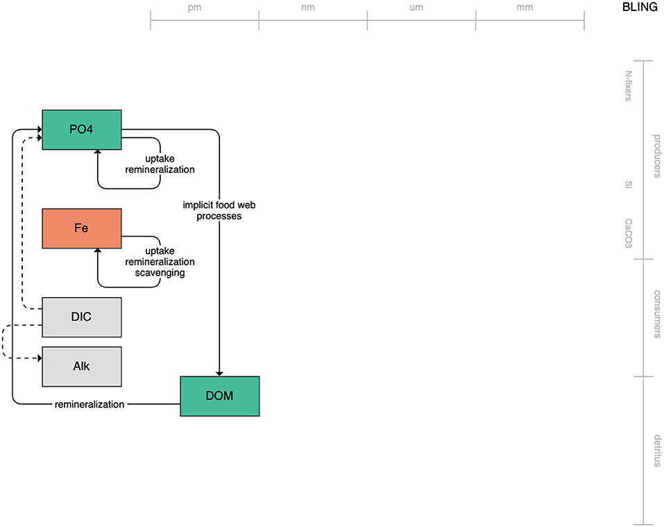
Figure 1. Schematic for the BLING model. Figures 1–12. Schematics for the CMIP6 ESMs. Boxes indicate state variables, and solid arrows represent fluxes between state variables; dashed lines indicate that the rate of change of one state variable is calculated proportionately to another. Colors indicate the base element for each state variable, with blue, green, pink, orange, and gray representing nitrogen, phosphorous, silicon, iron, and carbon, respectively. State variable boxes are positioned vertically based on functional role, indicating whether the functional group includes producers (and within that, subcategories of nitrogen fixers, Si-users, and CaCO3-users), consumers, or detritus. Horizontal position indicates the approximate mean size of the cells/bodies/particles represented by each state variable.

The second category of models includes traditional NPZD models that include single phytoplankton, zooplankton, and detrital compartments. This category includes CMOC of CCCMA (Figure 2), WOMBAT of CSIRO (Figure 3), and MRI-NPZD model of the Japanese Meteorological Research Institute (Figure 4). The HAMOCC model (Figure 5), variants of which are run within the models of Norwegian Climate Center and Max Planck Institute, also uses a single state variable each for phytoplankton and zooplankton but separates detritus into dissolved and particulate detritus. The OECO of MIROC model (Figure 6) uses two phytoplankton functional groups to distinguish nitrogen-fixing diazotrophs from non-nitrogen-fixing producers but otherwise falls into this simpler category of model. While several models in this category consider multiple limiting macronutrients (nitrogen, phosphorous, and silicon) and micronutrients (iron), they assume constant stoichiometric ratios of these nutrients within the food web.

FIGURE 2

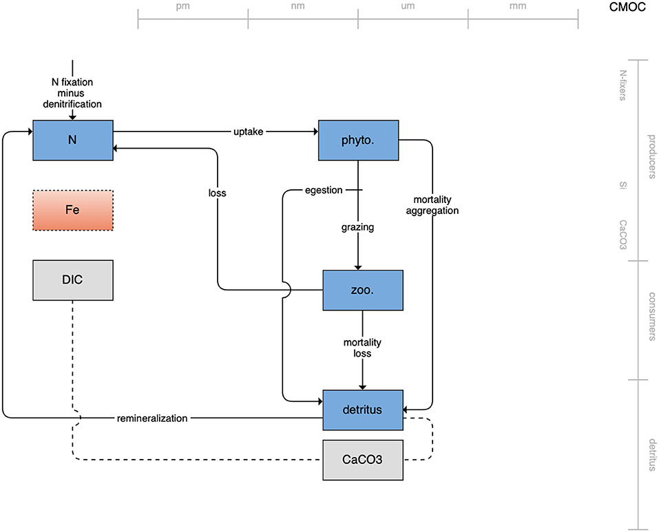
Figure 2. Schematic for the CMOC model. See Figure 1 caption for details.

FIGURE 3

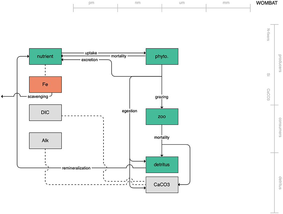
Figure 3. Schematic for the WOMBAT model. See Figure 1 caption for details.

FIGURE 4

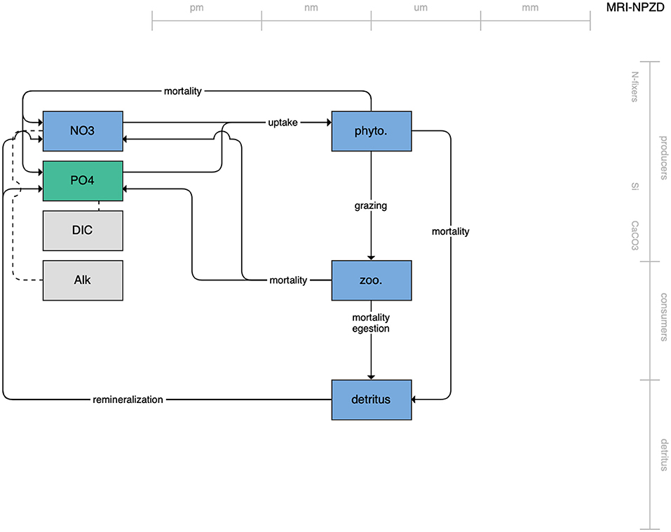
Figure 4. Schematic for the MRI NPZD model. See Figure 1 caption for details.

FIGURE 5

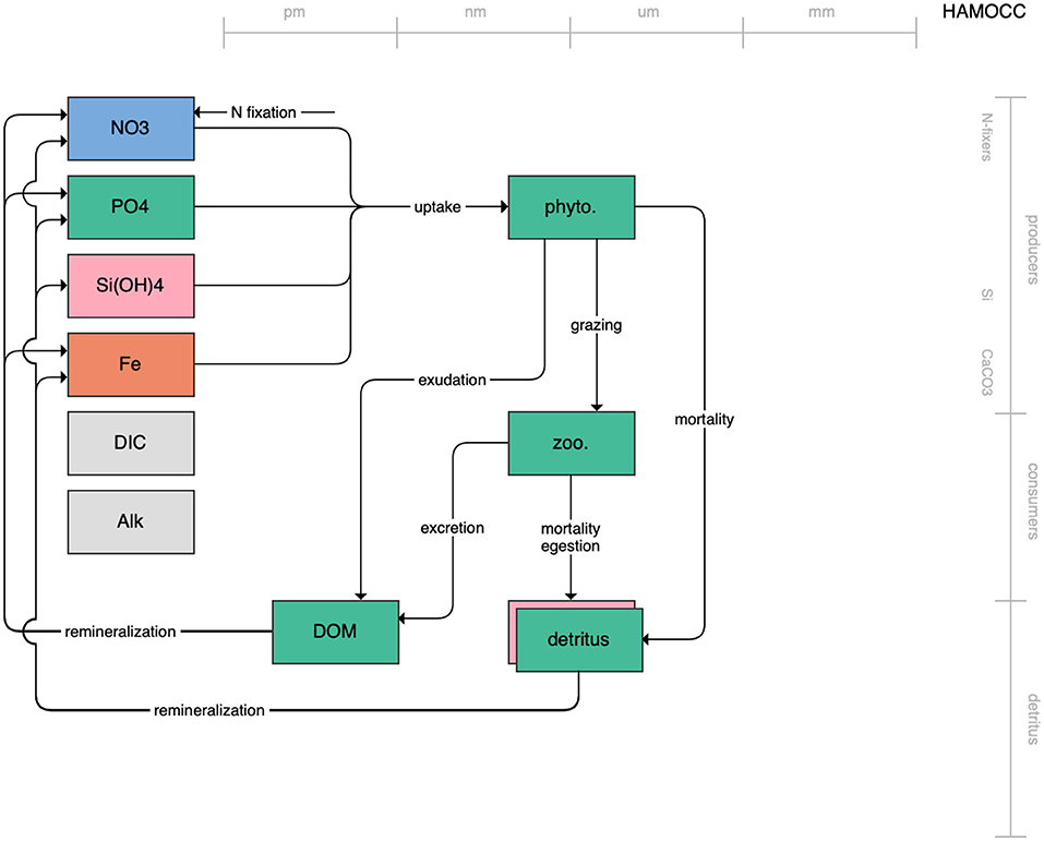
Figure 5. Schematic for the HAMOCC model. See Figure 1 caption for details.

FIGURE 6

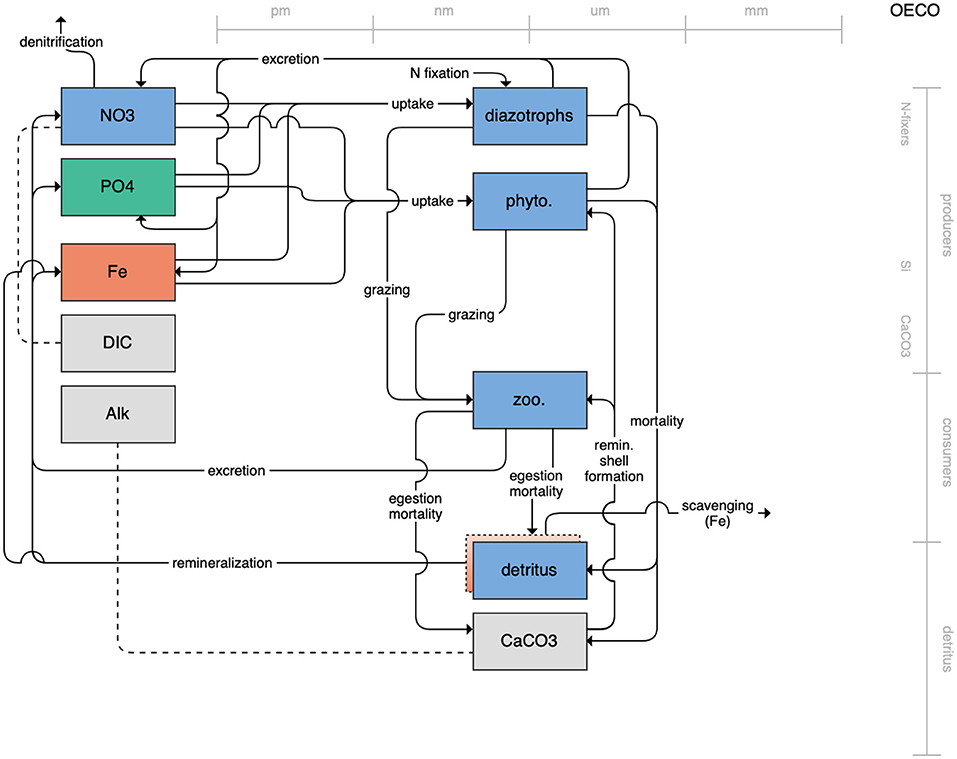
Figure 6. Schematic for the OECO model. See Figure 1 caption for details.

On the more complex end of the spectrum, the remaining models partition phytoplankton, zooplankton, and detritus into multiple state variables. This group of models includes PISCES (Figure 7), which is used in both the CNRM and IPSL models; COBALT of GFDL (Figure 8); CanOE of CCCMA (Figure 9); NOBM of NASA Goddard (Figure 10); MEDUSA of the UK (Figure 11); and MARBL of the CESM model (Figure 12). Phytoplankton within these models are separated into 2–4 functional groups; functional groups are typically defined based on their interactions with different nutrient pools, their size, and their accompanying influence on metabolic rates, and in the case of the NOBM model, by optical properties. Size is also one of the primary features used to separate zooplankton functional groups due to the role of body size in determining prey preferences, metabolic rates, and the partitioning of mortality and metabolic byproducts into the different detrital pools. Non-living organic material is categorized by either size or lability. This more complex category of models typically allows for variable stoichiometry within the primary producer and detrital state variables; most assume a fixed stoichiometry for consumers, though the MARBL model is an exception to this. Allowing for variable vs. fixed stoichiometry has been demonstrated to significantly impact simulated trophic transfer efficiency under climate change scenarios (Kwiatkowski et al., 2019), so this additional complexity may be particularly important for LMR applications.

FIGURE 7

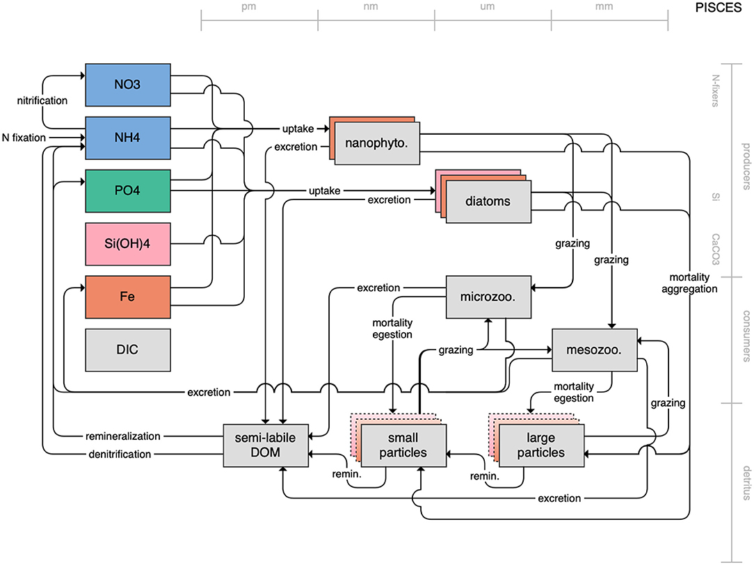
Figure 7. Schematic for the PISCES model. See Figure 1 caption for details.

FIGURE 8

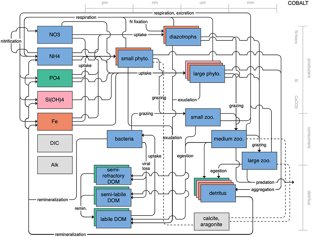
Figure 8. Schematic for the COBALT model. See Figure 1 caption for details.

FIGURE 9

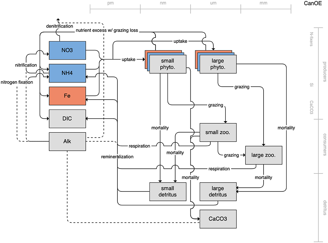
Figure 9. Schematic for the CanOE model. See Figure 1 caption for details.

FIGURE 10

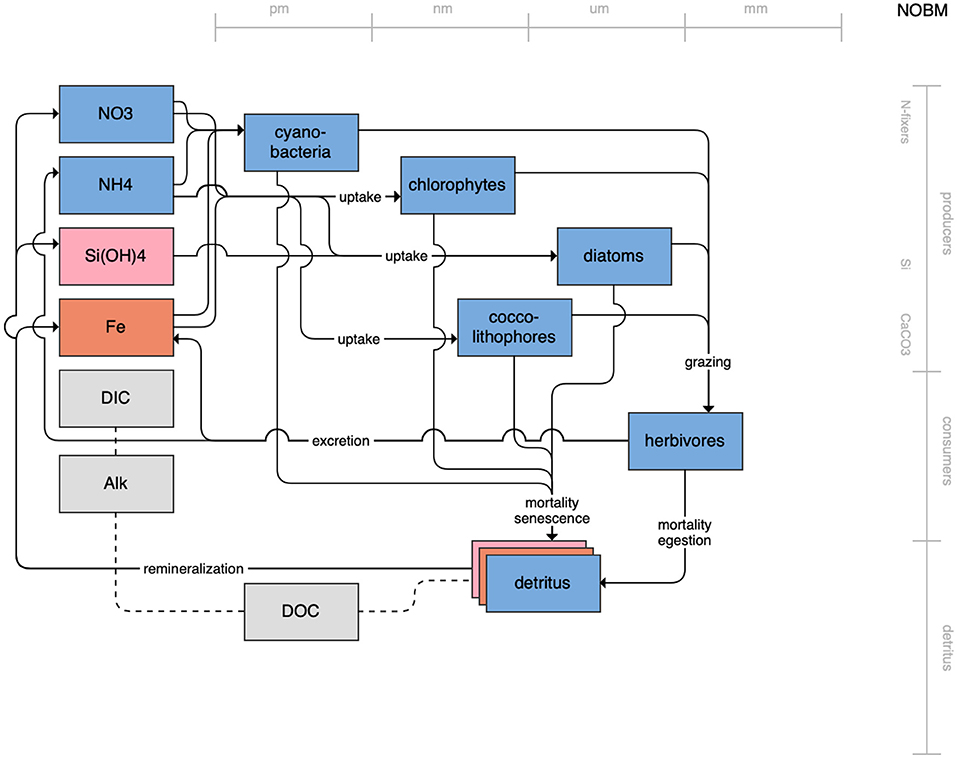
Figure 10. Schematic for the NOBM model. See Figure 1 caption for details.

FIGURE 11

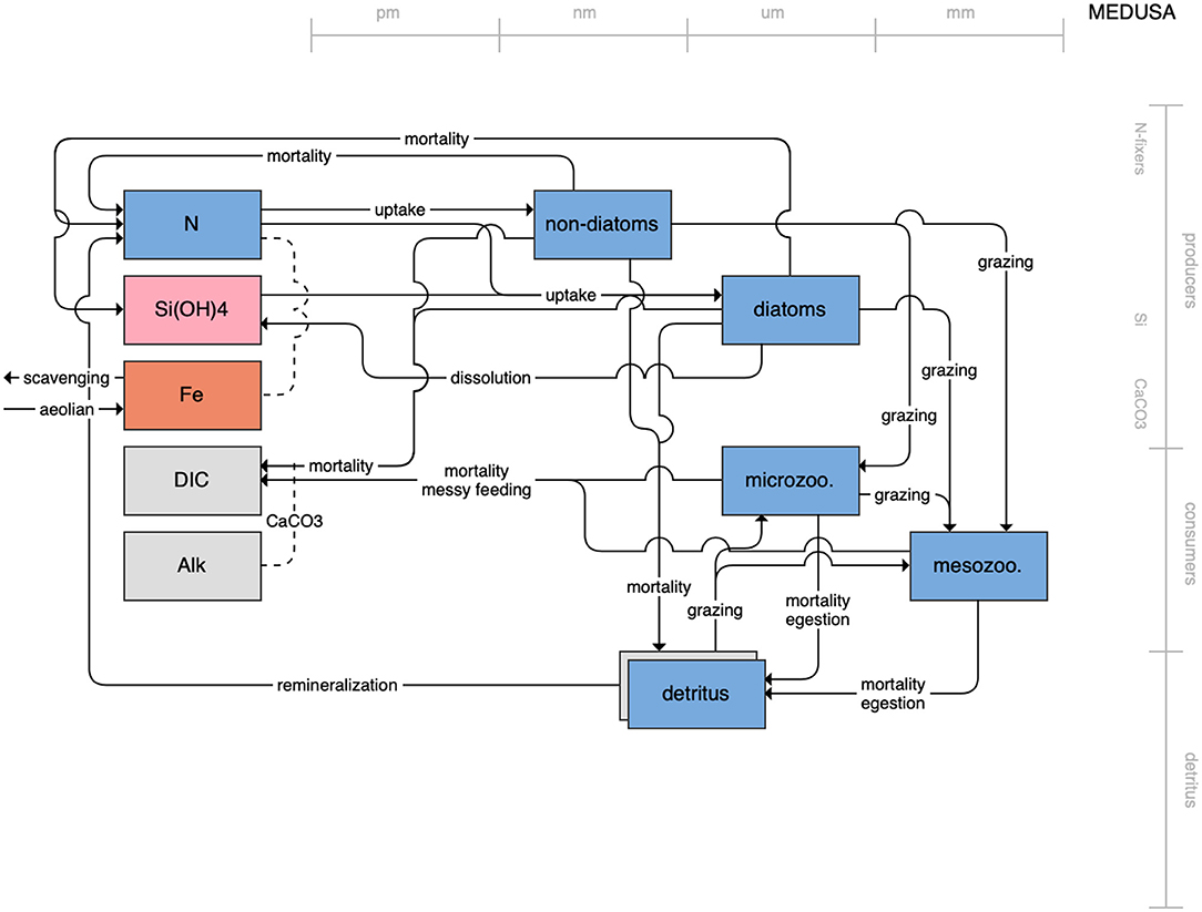
Figure 11. Schematic for the MEDUSA model. See Figure 1 caption for details.

FIGURE 12

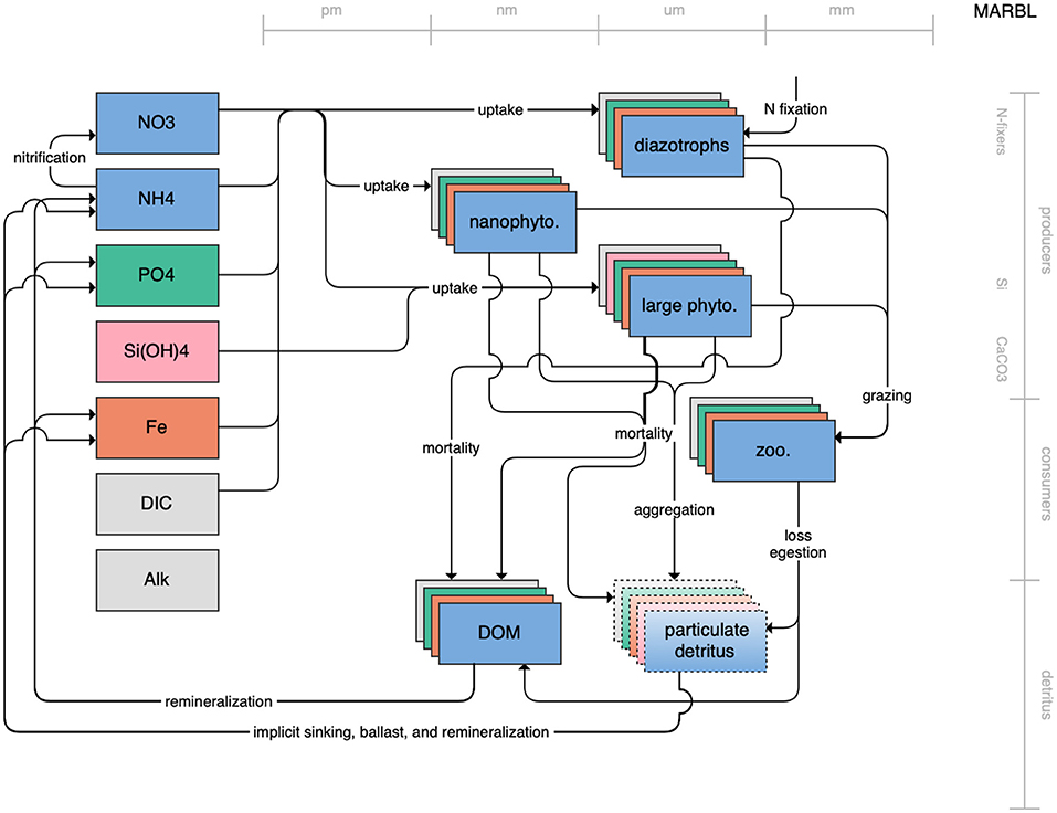
Figure 12. Schematic for the MARBL model. See Figure 1 caption for details.

With an increase in the number of state variables in a model comes an increase in the complexity of connections between those state variables, and the number of parameters (each with its own uncertainty) necessary to constrain them. These connections include both the pathways that pass biomass and energy to higher trophic levels and the pathways that lead to export from or recycling of nutrients in the surface waters. A more complex model may be better able to capture the shifts in community composition and prey quality that are key to simulating upper trophic level recruitment and survival. For example, environmental conditions that favor larger phytoplankton species often lead to higher transfer efficiencies to upper trophic level species, while small phytoplankton production is often directed toward smaller grazers and the microbial loop (Azam et al., 1983; Armengol et al., 2019). These potential shifts in energy pathways are of particular interest in LMR applications that focus on plankton groups in their role as “fish food” rather than as regulators of biogeochemical pathways (Rose et al., 2010). Van Oostende et al. (2018) also found that adding an additional phytoplankton group to their model of the California Current system led to better resolution of both chlorophyll maxima and coastal hypoxia. Likewise, explicitly resolving different zooplankton size classes can increase the types of ecosystem analyses that are possible based on ESM output. For example, the GFDL COBALT model is essentially a more ecosystem-heavy version of its predecessor, TOPAZ (Dunne et al., 2013). By adding three explicit zooplankton groups (and bacteria) in place of the implicit zooplankton parameterization found in TOPAZ, COBALT has been able to be used for a diverse set of LMR applications: to model and predict fisheries catch in LMEs (Stock et al., 2017; Park et al., 2019), to couple to offline models to examine distributions of fish functional types (Petrik et al., 2019) and the impact of jellyfish on the global carbon cycle (Luo et al., 2020), and to examine the impacts of migration and light-dependent grazing on the vertical distribution of carbon, nutrients, and chlorophyll (Bianchi et al., 2013; Moeller et al., 2019). Greater resolution of detrital components may allow for better resolution of the different time scales over which material may be exported to deep water, transported into or out of a region of interest, or returned to the nutrient pools. These remineralization pathways can directly affect the local availability of nutrients that, in turn influence rates of primary production. This is particularly true in shallow shelf systems, where nutrients exported below the mixed layer may be reintroduced to surface waters by mixing events (Huang et al., 2015; Flynn et al., 2020). Particle export ratios and fluxes to the benthic ecosystems have also been shown to be better predictors of fisheries productivity (Friedland et al., 2012; Stock et al., 2017) and of the composition of fish communities (Van Denderen et al., 2018; Petrik et al., 2019) than net primary productivity alone. It is important to note, however, that while the state variables and processes included in more complex models often reflect our best estimation of the Earth system processes that influence both lower and upper trophic level dynamics, the added complexity does not necessarily impart greater skill (Séférian et al., 2020).

Phytoplankton Growth Limitation Terms

Primary productivity rates and phytoplankton biomass are some of the most commonly extracted ESM variables of interest to LMR end users. As the base of the food web, plankton production often determines the characteristics of the food web that can be supported in a given region. Changes to the magnitude, community composition, or timing of spring and fall blooms may impact the survival of upper trophic level species (Platt et al., 2003; Durant et al., 2007; Schweigert et al., 2013; Malick et al., 2015; Asch et al., 2019). Because the most important process controlling interior ocean pH is organic matter cycling, the processes limiting primary production also influence the pH (Lauvset et al., 2020). Acid-base reactions involved in nutrient uptake also have an impact on both pH and alkalinity (Wolf-Gladrow et al., 2007). Therefore, model structure related to the regulation of primary production may influence many of the key properties of interest to LMR end users.

Phytoplankton growth rates vary based on a number of factors, chief among them temperature, light, and availability of both the macronutrients and micronutrients necessary for growth. Within ESMs, maximum phytoplankton growth rate is typically modeled as a temperature-dependent maximum potential growth rate modulated by limitation terms (with values ranging from 0 to 1) that reduce that rate based on limited nutrient supplies and light. While this concept is consistent across all CMIP6 models, the exact implementation of each limitation term and the manner in which they interact vary from model to model. We will address variations in the temperature-dependent maximum growth rate in section 3.3 and focus here on the light- and nutrient-limitation terms.

Nutrient-limitation terms typically fall into one of two broad categories. The first category calculates limitation as a function of ambient nutrient concentration. The majority of the CMIP6 ESMs use this approach for limitation terms related to the macronutrients (i.e., nitrogen and phosphate) (Tables 3, 4). Monod curves (Monod, 1942), also referred to as Michaelis-Menten curves due to their functional equivalence to the enzyme kinetics equation (Michaelis and Menten, 1913), define limitation in terms of a half-saturation constant (K_X). This is the most common nutrient-limitation term equation found in the CMIP6 ESMs. The MPI-NPZD model instead opts for an optimal uptake kinetics approach (Smith et al., 2009) that accounts for tradeoffs in nutrient encounter rates and assimilation rates; like the Monod curve, this approach assumes growth rate is a function of external nutrient concentration. The second category of limitation uses an internal cell quota model. A quota-model limitation term is based on the internally stored concentration of a particular element rather than the ambient concentration, and it allows for uptake and storage of one or more nutrients beyond immediate needs. This style of limitation term can be more appropriate when dealing with elements like silicon and iron; Fe:C and Si:C ratios can vary much more widely within cells relative to macronutrients like N and P. Within the CMIP6 suite, COBALT and PISCES use quota models for iron limitation. BLING also uses a variant on the quota model for iron limitation, adapted to infer cell quota from uptake rates. CanOE uses a quota model for both nitrogen and iron uptake.

TABLE 3

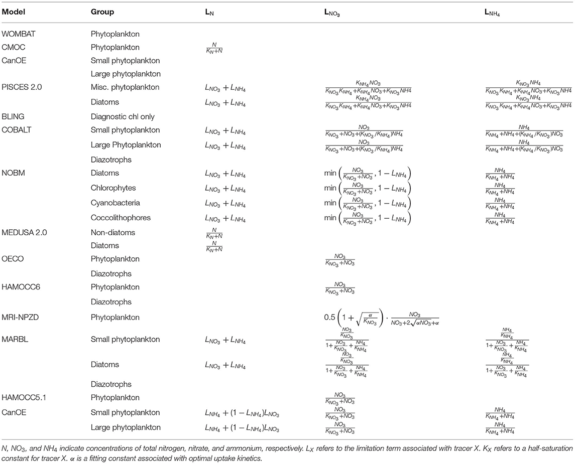
Table 3. Nitrogen nutrient-limitation factors across all CMIP6 ESMs.

TABLE 4

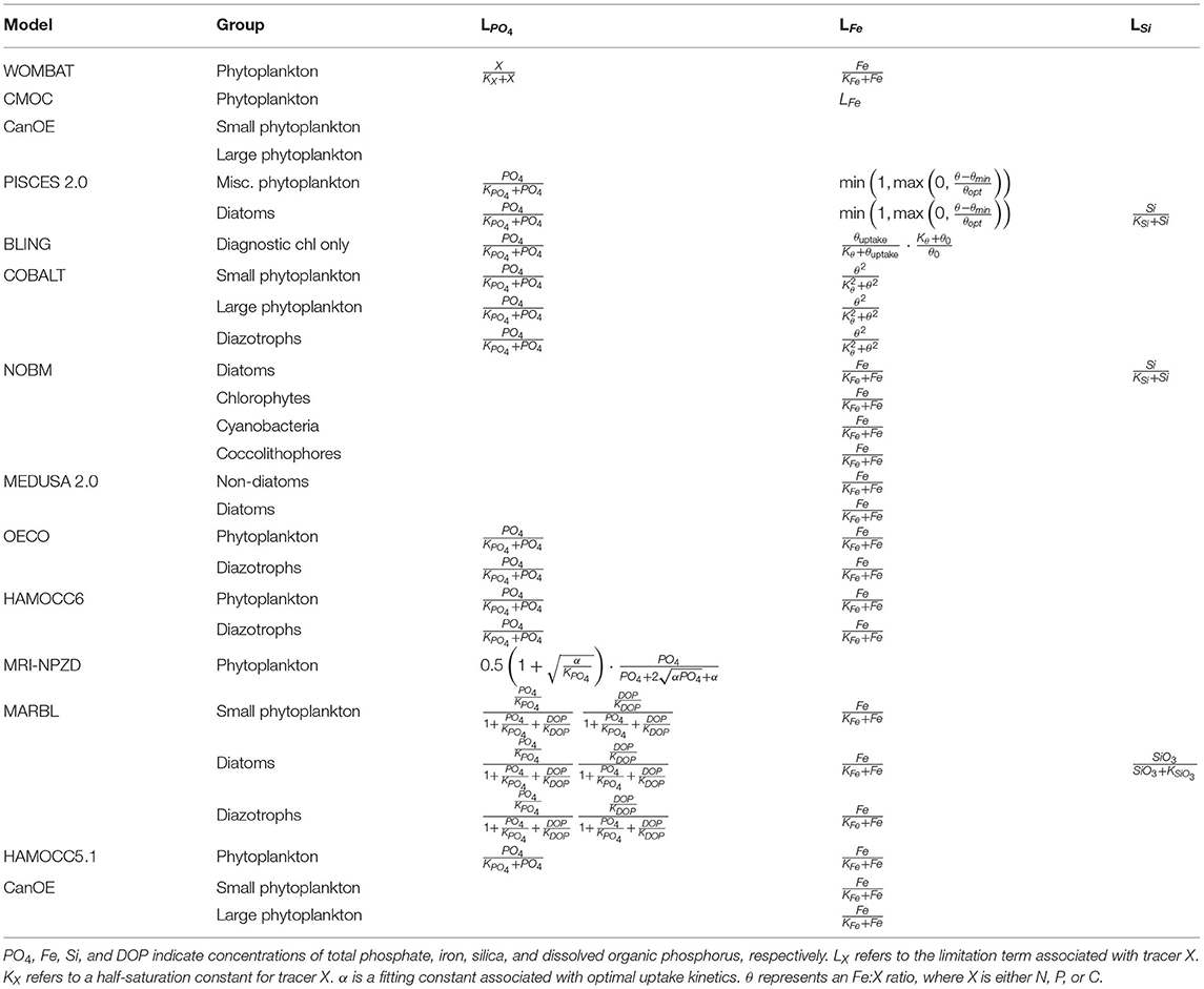
Table 4. P, Fe, and Si nutrient-limitation factors across all CMIP6 ESMs.

Phytoplankton can acquire nitrogen from a variety of different organic and inorganic compounds, and the sources that contribute to the nitrogen limitation term of each model provide additional potential for model structural divergence (Table 3). Non-nitrogen-fixing phytoplankton typically acquire nitrogen from two primary forms: nitrate or ammonium. The relative use of new (nitrate-based) vs. regenerated (ammonium-based) nutrient sources for production reflects whether an ecosystem is dominated by larger phytoplankton species that pass energy up the food chain and contribute to higher export ratios of carbon from surface to deep water, or whether the ecosystem is dominated by smaller phytoplankton with production primary recycled within the microbial loop (Dunne et al., 2005). Due to its reduced state, ammonium is more readily utilized by phytoplankton for growth (Gruber, 2008). In addition, the presence of high concentrations of ammonium can directly inhibit the uptake of nitrate (O'Neill et al., 1989; Dortch, 1990; Frost and Franzen, 1992; Paulot et al., 2015). Therefore, the limitation terms of many of the CMIP6 ESMs are formulated to favor ammonium uptake over nitrate uptake and to adjust nitrate uptake in the presence of ammonium. PISCES, COBALT, CanOE, MARBL, and NOBM track the separate use of NH₄ vs. NO₃, with total nitrogen limitation being a sum of the two individual limitation terms. COBALT and PISCES account for both ammonium preference and its inhibition on nitrate, as well as inhibition of ammonium uptake of nitrate in the presence of very high concentrations of nitrate (O'Neill et al., 1989). NOBM and CanOE impose a preference for NH₄ over NO₃ but do not apply any inhibition terms to the uptake of either nutrient. OECO, HAMOCC5.1, and HAMOCC6 track NO₃ only. CMOC and MEDUSA, meanwhile, track only a single pool of nitrogen. A number of the ESMs also account for nitrogen fixation. Nitrogen fixers are able to transform N₂ gas into fixed nitrogen (NH₄), and in models they are typically differentiated from other phytoplankton groups through the elimination of an N-limitation term in their growth equation. COBALT, OECO, HAMOCC6, and MARBL all simulate nitrogen-fixing diazotrophs in this manner. The NOBM model instead uses an additional factor to increase the N-limited growth rate of the cyanobacteria group when N is low, representing a shift within the functional group from non-nitrogen-fixing to nitrogen-fixing cyanobacteria. CMOC simulates only a single nutrient pool and single phytoplankton group but provides a flux of nitrogen into its surface nutrient pool based on implicit parameterizations of diazotrophic bacteria. Likewise, CanOE parameterizes nitrogen fixation as an input source to the ammonium field, dependent on light, temperature, and iron concentration and inhibited by high inorganic nitrogen.

Phytoplankton growth rates can also be very sensitive to even small variations in light and light sensitivity (e.g., Walsh et al., 2003). A number of different empirical curves, known as photosynthesis-irradiance (PI or PE) curves, have been proposed to quantify the relationship between solar irradiance and photosynthesis (e.g., Jassby and Platt, 1976; Platt and Jassby, 1976; Platt et al., 1980). Within the CMIP6 suite, NOBM uses the simplest form, identical to its Monod nutrient-limitation terms, with a functional-group-specific light half-saturation parameter. MEDUSA, OECO, and MPI-NPZD use a hyperbolic tangent curve (Smith, 1936; Jassby and Platt, 1976):

$\begin{array}{ll}\frac{{\mu }_{max}(T)\alpha I}{\sqrt{{({\mu }_{max}(T))}^2+{(\alpha I)}^2}}& (1)\end{array}$

where μ_max(T) is the light- and nutrient-replete growth rate at temperature T, α describes the initial slope of the PI curve, and I is the solar irradiance.

The remaining models base their PI curves on that of Geider et al. (1997):

$\begin{array}{ll}1-exp\left(\frac{-{\alpha }_{chl}{\theta }_{chl}I}{{\mu }_{max}(T,N)}\right)& (2)\end{array}$

where α_chl is the chlorophyll-specific initial slope of the PI curve, θ_chl is the chlorophyll-to-carbon (chl:C) ratio, and μ_max(T, N) is temperature- and nutrient-mediated growth rate under light-replete conditions. In this form, the light-limitation curve is a function of nutrient and temperature limitation, such that nutrient concentration and temperature play both a direct and indirect role in modulating growth. The WOMBAT model simplifies this relationship by using μ_max(T) in place of μ_max(T, N). By introducing a chl:C parameter, this function captures the process of photoadaptation, where phytoplankton increase their chlorophyll levels to compensate for low light levels. COBALT and BLING account for the effects of both irradiance and nutrient limitation when calculating the θ_chl value. MARBL and CanOE compute a prognostic chlorophyll with chlorophyll biosynthesis calculated as a function of light and nutrient availability (after Geider et al., 1998). Within CMOC, PISCES, NOBM, and MEDUSA2, θ_chl is a function of irradiance only. WOMBAT, OECO, and HAMOCC do not account for variation in chl:C ratios in their light-limitation factors.

A final structural difference arises in how each model applies colimitation from nutrients, light, and temperature. In general, primary productivity models use one of two models: a minimum limiting factor model (Liebig and Playfair, 1843) or a multiplicative model. All models in the CMIP6 suite use a minimum model across nutrients but vary regarding the colimitation with light. PISCES, COBALT, MARBL, and HAMOCC calculate a separate minimum limiting nutrient factor and light limitation factor, both applied multiplicatively to a temperature-dependent maximum uptake rate [note that for the models that use the Geider et al. (1997) nutrient-mediated light formulation, and this implementation in effect determines whether there is enough light to reach the nutrient-limited rate]. CanOE uses a similar implementation but with the nutrient-limitation factor calculated as the minimum of N- and Fe-based cell quota terms rather than using the same limitation term as for uptake. CMOC, NOBM, OECO, MRI-NPZD, and WOMBAT calculate a single limiting factor across both nutrient and light limitation and apply this to a temperature-dependent uptake rate.

Temperature Influence on Biological Rates

Variations in temperature dependence at various trophic levels, both within a single model and across models, can play a key role in determining how primary and secondary production rates in each ESM respond relative to each other both seasonally and under long-term climate change scenarios. This in turn can influence whether an increase in temperature leads to higher or lower trophic transfer efficiencies (i.e., fraction of production at one trophic level relative to one below it), which is of particular interest when quantifying how changes affect upper trophic level species. For example, Reum et al. (2020) found that temperature dependency assumptions were a key source of intermodel uncertainty in their examination of the impact of climate change on the Bering Sea food web.

The exponential scaling of maximum plankton growth rate with temperature was first reported by Eppley (1972), and the resultant “Eppley-curve” is an empirical function widely used to estimate primary productivity from satellites (Morel, 1991; Behrenfeld and Falkowski, 1997) and incorporated in models (e.g., Stock et al., 2014). The majority of the CMIP6 models formulate their temperature-dependent factors using an Eppley-style exponential curve, with coefficients that reflect updated data compilations (e.g., Brush et al., 2002; Bissinger et al., 2008).

The Arrhenius-Van't Hoff equation (Arrhenius, 1915) is an alternative to the Eppley function that has traditionally been used to describe the rates of chemical reactions. However, it can also be used to describe biological rates, as metabolic rates are typically limited by a rate-limiting biochemical step, such as Rubisco carboxylation for autotrophic growth and adenosine triphosphate (ATP) synthesis for heterotrophic growth (Gillooly et al., 2001; Brown et al., 2004). These ideas have been incorporated into the metabolic theory of ecology (MTE; Brown et al., 2004) that broadly describes how metabolic rates scale with biomass and temperature. MTE uses the activation energy (E_a) of the rate-limiting enzymatic reaction to describe the temperature dependence of metabolic rates. This mechanistic derivation of temperature limitation leads to a similarly-shaped temperature vs. rate curve as the more empirically derived Eppley formulation; though within the temperature range of most biological processes (0–40C), there can be up to a 10–15% difference in rates when using the Eppley formulation vs. the Arrhenius (or MTE) equation (Gillooly et al., 2002). Within the CMIP6 suite, CMOC and CanOE rely on the Arrhenius-Van't Hoff equation for their temperature sensitivities.

The sensitivity of the various temperature curves used within the CMIP6 models can be compared by looking at the Q10 value, i.e., the acceleration of a given reaction when the temperature is increased by 10°C. While the exact equations used vary, all models within the CMIP6 suite apply a similar temperature dependence to phytoplankton growth rate, with similar Q10 values (Table 5).

TABLE 5

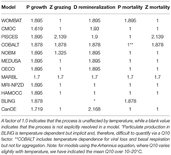
Table 5. Q10 factor associated with various model processes for a given ESM.

However, the models differ when it comes to the effect of temperature on other processes. In PISCES, COBALT, NOBM, and MARBL, zooplankton grazing rates are also temperature dependent. Within PISCES, the zooplankton grazing rate is more strongly influenced by temperature than phytoplankton nutrient uptake, while in NOBM, the reverse is true; COBALT and MARBL apply the same Q10 factors to both processes. In the remaining models, the zooplankton grazing rate is unaffected by temperature. Detrital remineralization is also temperature dependent in all models except for MRI-NPZD and HAMOCC. Within CMOC, CanOE, and PISCES, the detrital remineralization Q10 values are higher than those for phytoplankton uptake rate, while in the remaining models the Q10 factors are the same. The temperature dependence of nutrient recycling and the microbial loop have been highlighted as a key source of uncertainty in projections of both the magnitude and direction of net primary productivity under climate change (Taucher and Oschlies, 2011). Finally, phytoplankton and zooplankton mortality rates are temperature dependent in a handful of models. WOMBAT, MARBL, BLING, and COBALT include temperature terms in their phytoplankton mortality rates, while PISCES, COBALT, and MARBL apply similar terms to zooplankton mortality.

From the perspective of modeling of higher trophic levels such as fish, the assumptions regarding temperature effects are critical. While warming may increase overall primary productivity, limits on the zooplankton grazing rate and increases in zooplankton mortality may serve as bottlenecks that prevent increased primary production from reaching fish and higher trophic levels. Likewise, the relative response of remineralization processes may alter the balance between benthic vs. pelagic energy pathways. Laufkötter et al. (2017) found that changes to the temperature dependence of remineralization rates within an ESM could strongly influence surface nutrient concentration and the extent of oxygen minimum zones. Therefore, assumptions of the ESM can strongly influence predictions when coupled to higher trophic level models.

Zooplankton Functional Response

Zooplankton functional response is one area where the CMIP6 models tend to converge structurally, with all models using either a type 2 or type 3 functional response (Table 6). A type 2 functional response, which is used in the NOBM, CanOE, MARBL, and HAMOCC models, is defined as one where grazing rate increases linearly at low prey biomass and approaches a threshold rate at high prey biomass; the functional form is concave down everywhere (Gentleman et al., 2003). A type 3 functional response is similar, except for the presence of an inflection point that decreases predator grazing rates at low prey biomass relative to a type 2 function (Gentleman et al., 2003). Sigmoidal type 3 functional responses are used in WOMBAT, CMOC, MEDUSA, OECO, and MRI-NPZD; PISCES uses a type 3 threshold model instead. COBALT falls in between, using a type 2 response but with a small prey biomass adjustment to limit grazing at very low prey concentrations. This limited number of functional response forms contrasts with the many functional responses applied in ecosystem models for higher trophic levels, such as those summarized in Hunsicker et al. (2011).

TABLE 6

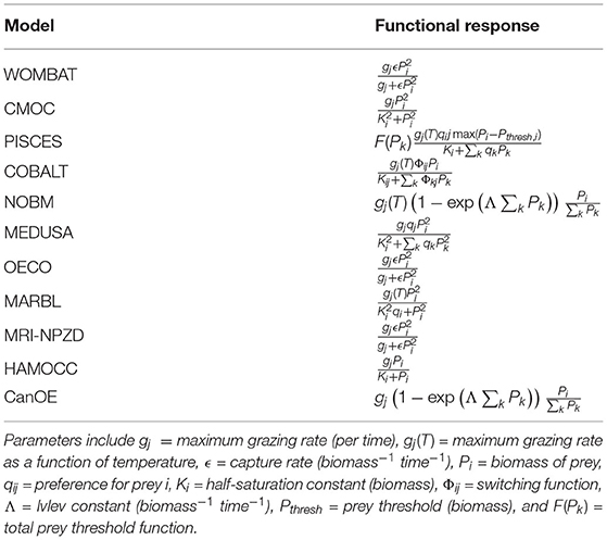
Table 6. Per unit biomass grazing functional responses of predator j on prey i, with other available prey groups k.

Where grazers can feed on multiple prey groups (including either phytoplankton, zooplankton, or detrital prey sources), many of the models calculate grazing rates using a single-resource model, where the grazing rate on a particular prey species is determined independently of whether other prey are present. PISCES, COBALT, NOBM, MEDUSA, and CanOE do consider total prey availability when calculating grazing rates. NOBM and CanOE calculate grazing as a function of total prey, with predation distributed across the prey species proportional to prey availability. MEDUSA and PISCES both use prey preferences, such that grazing rate is a function of both prey availability and the relative preference of predator for each prey species. COBALT uses a similar preference-based model but adds a switching function such that predator preference for prey increases when that prey is abundant.

Detrital Remineralization

The biological carbon pump is a collection of processes that determine the export and associated remineralization of particulate organic carbon (POC) produced by biological activity at the ocean surface (Passow and Carlson, 2012). These processes play a key role in the global carbon cycle; because carbon is assimilated by biological processes in the surface waters and then sequestered at depth, through both the soft-tissue pump (sinking of organic matter) and carbonate pump (sinking of carbonate mineral shells), the ocean takes up far more atmospheric CO₂ (Sarmiento and Gruber, 2006, and citations within) than through the solubility pump alone. The strength of the biological pump is estimated to be between 5 and 13 Pg C yr⁻¹ (Laws et al., 2000; Dunne et al., 2007; Henson et al., 2011), though models from the CMIP5 era ranged in the lower end of those estimates (5–8 Pg C yr⁻¹) (Laufkötter et al., 2016).

In addition to the role this process plays in the global carbon cycle, detrital remineralization can affect regional patterns in nutrient concentration. The speed at which material is transported from the surface waters to below the mixed layer may affect nutrient limitation and, therefore, primary production. Particularly in shallow coastal environments, how detrital remineralization is simulated and parameterized may influence whether organic material is recycled within the water column, is fed into a benthic food web, or is subject to burial.

Aside from the models that treat organic matter remineralization in a highly generalized fashion (e.g., BLING, CMOC, MRI-NPZD), CMIP6 models generally treat detrital remineralization in similar ways, though specific implementation may vary. In general, particulate organic matter in models is produced through a combination of phytoplankton loss and aggregation processes, and zooplankton grazing and mortality (Laufkötter et al., 2016). The specific type of detrital particle impacts the particle sinking speed or remineralization rates, which are correlated quantities. Particles that sink faster and/or are protected from bacterial remineralization have lower remineralization rates and, thus, longer remineralization length scales (defined as the depth at which 63% of the organic matter has been converted to inorganic forms). A key factor determining whether a detrital particle is protected or is faster-sinking is the presence of ballast materials (lithogenic particles, biogenic silica, and calcium carbonate), originating from organisms such as diatoms, coccolithophores, and foraminifera, and dust deposition (Armstrong et al., 2002; Francois et al., 2002; Klaas and Archer, 2002; Dunne et al., 2007). ESMs focus on characterizing ballast materials properly in order to achieve a representation of both ballasting and non-ballasting POM remineralization at depth, often relying on a variant of the Klaas and Archer (2002) mineral ballasting model.

The treatment of ballasting and non-ballasting particulate organic matter in CMIP6 models can then be divided into those that use a flux attenuation scheme (MARBL, HAMOCC, and OECO) and those that have sinking particles, whether in one or multiple size classes (COBALT, CanOE, PISCES, MEDUSA, and NOBM; also see the categorization of Séférian et al., 2020). In a flux attenuation scheme, organic material losses such as non-predatory mortality, egestion, and aggregation are collected into an implicit detrital pool that is then redistributed across depth to various inorganic nutrient pools based on depth profiles of remineralization rates. Treatment of ballast materials in this case results in the “hard POM” distributing more evenly throughout deeper depths, associated with their (implicitly) faster sinking speeds (e.g., Abell et al., 2000). In the remaining schemes, the organic material losses flow to one or more detrital state variables within the model grid cell in which the loss process occurs; the detrital state variables are then subject to vertical sinking. For the size-differentiated detrital models, loss fluxes are typically categorized based on the size and type of source material, with larger and ballasted particles sinking more quickly than smaller and non-ballasted ones. In the majority of models, these size- and type-specific sinking speeds are constants though some models also take the effect of temperature on sinking speed and/or remineralization into account (e.g., NOBM and COBALT).

River Runoff

For regional LMR applications, river runoff can be important due to its impact on a coastal circulation, vertical stratification, salinity, nutrient and dissolved organic matter concentration, biological production, and carbon chemistry (e.g., Dagg and Breed, 2003; Lohrenz et al., 2008; Gomez et al., 2019). Physical impacts include buoyancy-driven coastal currents such as the Alaska Coastal Current and associated mesoscale eddies (Stabeno et al., 2016). Large riverine inputs of nutrients can lead to coastal eutrophication, and the subsequent remineralization of organic matter can promote hypoxia and enhanced acidity near bottom, especially in regions with poor ventilation and weak buffer capacity (Bianchi et al., 2010; Cai et al., 2011, 2017; Fennel et al., 2016). In addition, the biogeochemical signature of land-influenced river water is distinct from that of ocean-derived water. The usually more acidic water from rivers determines decreased aragonite saturation levels (Duarte et al., 2013), increasing the vulnerability of coastal regions to ocean acidification. Riverine input of dissolved iron can have a substantial impact on coastal production (Coyle et al., 2019).

Within the CMIP6 suite of models, a wide variety of approaches are used to resolve riverine processes (Table 7). Freshwater fluxes in many models are calculated as part of the coupled ESM. When this is the case, the river fluxes are a function of processes within the atmosphere, ocean, and land components of the model, and they respond to changes in the simulated climate. In other models, freshwater fluxes are derived from an external data set, such as the river runoff climatologies of Dai and Trenberth (2002) and Dai et al. (2009). Many of the global models add runoff as a surface flux to the ocean within a specified distance from the coast (Griffies et al., 2016). This technique only partially compensates for the severely limited resolution of the true estuarine circulation and mixing (and consequent boundary currents) by coarse ocean model grids. Some of the CMIP6 models include significant improvements to the surface flux approach used in CMIP5. These include the following: (1) the estuarine box model technique (Sun et al., 2017) now incorporated into CESM2 (Danabasoglu et al., 2020) and (2) enhanced vertical mixing in coastal grid cells receiving riverine input, now incorporated into MOM6 of GFDL (R. Hallberg, pers. comm.).

TABLE 7

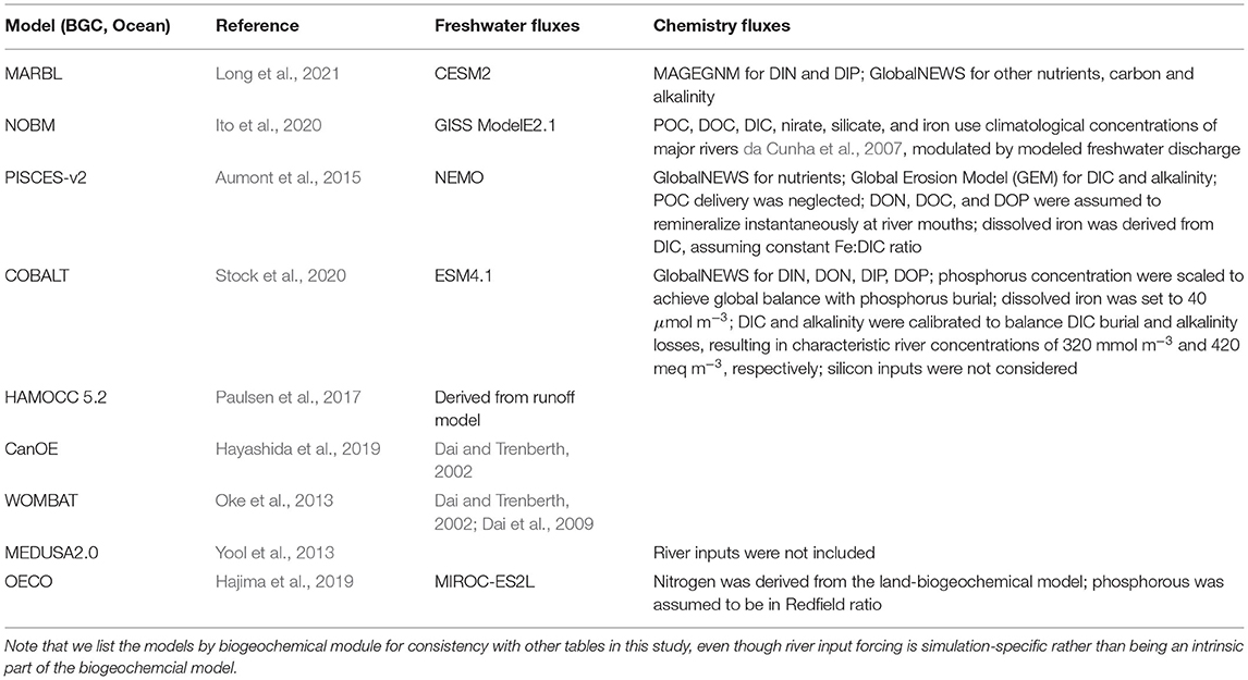
Table 7. River runoff treatment in the CMIP6 ESMs.

Biogeochemical riverine inputs, when included, primarily rely on external river export models, including the Integrated Model to Assess the Global Environment-Global Nutrient Model (IMAGE-GNM) (Beusen et al., 2015, 2016), the Global Nutrient Export from Watersheds (NEWS) model (Seitzinger et al., 2005; Mayorga et al., 2010), and the Global Erosion Model (GEM) (Ludwig and Probst, 1996).

Overall, the CMIP6 suite of ESMs does not represent the spatiotemporal variability in regional-scale riverine fluxes of either freshwater or of nutrients, DIC, and alkalinity well; they are typically designed to capture global-scale trends that may not be appropriate when focusing on smaller regional scales. For example, the GFDL ESM4 input forcing (coupled to COBALT) assumes a river DIC of 320 mmol m⁻³ and a river total alkalinity (TA) of 420 meq m⁻³; these values are defined to compensate for global DIC and TA losses such that mass balance within the biogeochemical model domain is maintained. However, observations suggest that river DIC is usually greater than river alkalinity (see Figure 8 in Moore-Maley et al., 2018). With respect to global river discharge datasets, Kearney (2019) found that the algorithms used to fill spatiotemporal gaps in river gauge measurements within the Dai and Trenberth (2002) dataset were inappropriate for snow-influenced rivers like those emptying into the Bering Sea. Fully coupling the biogeochemical processes connecting the ocean and land systems, including those associated with rivers, the benthic ecosystem, and the continental shelf, remains an outstanding task that ESMs have not yet been implemented. When applying global ESM results to highly river-influenced areas, LMR end users may need to carefully consider potential limitations like these.

Conclusions

Projections of changing climate, across both short and long timescales, are playing an increasingly important role in many LMR management strategies (Link et al., 2015). The ability of management frameworks to use ESM output may be dependent on the complexity of the ecosystem models used to support decision-making that can range from population dynamics models with no environmental covariates included, through to complex end-to-end ecosystem models incorporating movement, bioenergetics, and fishing fleet dynamics (Fulton et al., 2011; Marshall et al., 2019). However, as Ecosystem-Based Fishery Management becomes more widely implemented, assessment and management processes will likely become more able to ingest ecosystem indicators and ESM projections. Even if current frameworks are not able to easily include environmental covariates, they can still be considered using Management Strategy Evaluation or scenario planning (Haward et al., 2013; Punt et al., 2016; Surma et al., 2018).

To support this endeavor, LMR scientists and managers must not only have access to climate and biogeochemical model output but also understand the differences among models in terms of simulating key processes, resolution, etc. The complexity of the suite of models and the constraints on getting needed model output have thus far been a hindrance for using the model output for LMR science and management. This study provides a summary of some of the key points LMR end users may need to consider when using the CMIP6 suite of biogeochemical model output and also provides an entry point to the more in-depth descriptions found in the primary documenting literature for each model (see Table 2).

Author Contributions

KK conceived of and organized the manuscript, drafted text, and created the figures. KK, JL, and FG researched and summarized the CMIP6 model equations. All authors assisted in organizing, writing, and editing text.

Funding

Funding provided through NOAA's Integrated Ecosystem Assessment program. Funding sources for this paper are as follows: NOAA Marine Ecosystem Tipping Points Initiative (ED, JL), NOAA Ocean Acidification Program (FG), Future Seas I & II projects under NOAA's Coastal and Ocean Climate Applications and Climate and Fisheries Adaptation Programs: grant numbers NA17OAR4310268 and NA20OAR4310507 (BM, SK), NOAA's Climate Variability and Predictability and The Modeling, Analysis, Predictions, and Projections Programs: grant numbers NA20OAR4310405 and NA20OAR4310447 (MP), and NOAA's Integrated Ecosystem Assessment program (KK).

Conflict of Interest

The authors declare that the research was conducted in the absence of any commercial or financial relationships that could be construed as a potential conflict of interest.

The handling editor declared a past co-authorship with several of the authors IK, BM, MJ, SK, KK, MM, and PW-J.

Publisher's Note

All claims expressed in this article are solely those of the authors and do not necessarily represent those of their affiliated organizations, or those of the publisher, the editors and the reviewers. Any product that may be evaluated in this article, or claim that may be made by its manufacturer, is not guaranteed or endorsed by the publisher.

Acknowledgments

Thank you to our two reviewers as well as our two NOAA internal reviewers, Charles Stock and Ryan Rykaczewski, for their input to make this paper as strong as possible.

References

Abell, J., Emerson, S., and Renaud, P. (2000). Distributions of TOP, TON and TOC in the North Pacific gyre: Implications for nutrient supply in the surface ocean and remineralization in the upper thermocline. J. Marine Res. 58, 203–222. doi: 10.1357/002224000321511142

CrossRef Full Text | Google Scholar

Ainsworth, C. H., Samhouri, J. F., Busch, D. S., Cheung, W. W., Dunne, J., and Okey, T. A. (2011). Potential impacts of climate change on Northeast Pacific marine foodwebs and fisheries. ICES J. Mar. Sci. 68, 1217–1229. doi: 10.1093/icesjms/fsr043

CrossRef Full Text | Google Scholar

Armengol, L., Calbet, A., Franchy, G., Rodríguez-Santos, A., and Hernández-León, S. (2019). Planktonic food web structure and trophic transfer efficiency along a productivity gradient in the tropical and subtropical Atlantic Ocean. Sci. Rep. 9, 1–19. doi: 10.1038/s41598-019-38507-9

PubMed Abstract | CrossRef Full Text | Google Scholar

Armstrong, R. A., Lee, C., Hedges, J. I., Honjo, S., and Wakeham, S. G. (2002). A new, mechanistic model for organic carbon fluxes in the ocean based on the quantitative association of poc with ballast minerals. Deep Sea Res. Part II Top. Stud. Oceanogr. 49, 219–236. doi: 10.1016/S0967-0645(01)00101-1

CrossRef Full Text | Google Scholar

Arrhenius, S. (1915). Quantitative Laws in Biological Chemistry (London: G. Bell).

Asch, R. G., Stock, C. A., and Sarmiento, J. L. (2019). Climate change impacts on mismatches between phytoplankton blooms and fish spawning phenology. Global Chang. Biol. 25, 2544–2559. doi: 10.1111/gcb.14650

PubMed Abstract | CrossRef Full Text | Google Scholar

Aumont, O., and Bopp, L. (2006). Globalizing results from ocean in situ iron fertilization studies. Global Biogeochem. Cycles 20, 1–15. doi: 10.1029/2005GB002591

CrossRef Full Text | Google Scholar

Aumont, O., Ethé, C., Tagliabue, A., Bopp, L., and Gehlen, M. (2015). PISCES-v2: an ocean biogeochemical model for carbon and ecosystem studies. Geosci. Model Dev. 8, 2465–2513. doi: 10.5194/gmd-8-2465-2015

CrossRef Full Text | Google Scholar

Azam, F., Fenchel, T., Field, J. G., Gray, J. S., Meyer-Reil, L. A., and Thingstad, F. (1983). The ecological role of water-column microbes in the sea. Mar. Ecol. Prog. Ser. 10, 257–263.

Google Scholar

Barange, M. (2019). Avoiding misinterpretation of climate change projections of fish catches. ICES J. Mar. Sci. 76, 1390–1392. doi: 10.1093/icesjms/fsz061

CrossRef Full Text | Google Scholar

Behrenfeld, M. J., and Falkowski, P. G. (1997). Photosynthetic rates derived from satellite-based chlorophyll concentration. Limnol. Oceanogr. 42, 1–20.

Google Scholar

Beusen, A. H., Bouwman, A. F., Van Beek, L. P., Mogollón, J. M., and Middelburg, J. J. (2016). Global riverine N and P transport to ocean increased during the 20th century despite increased retention along the aquatic continuum. Biogeosciences 13, 2441–2451. doi: 10.5194/bg-13-2441-2016

CrossRef Full Text | Google Scholar

Beusen, A. H., Van Beek, L. P., Bouwman, A. F., Mogollón, J. M., and Middelburg, J. J. (2015). Coupling global models for hydrology and nutrient loading to simulate nitrogen and phosphorus retention in surface water-Description of IMAGE-GNM and analysis of performance. Geosci. Model Dev. 8, 4045–4067. doi: 10.5194/gmd-8-4045-2015

CrossRef Full Text | Google Scholar

Bianchi, D., Stock, C., Galbraith, E. D., and Sarmiento, J. L. (2013). Diel vertical migration: Ecological controls and impacts on the biological pump in a one-dimensional ocean model. Global Biogeochem. Cycles 27, 478–491. doi: 10.1002/gbc.20031

CrossRef Full Text | Google Scholar

Bianchi, T. S., DiMarco, S. F., Cowan, J. H., Hetland, R. D., Chapman, P., Day, J. W., et al. (2010). The science of hypoxia in the northern Gulf of Mexico: a review. Sci. Total Environ. 408, 1471–1484. doi: 10.1016/j.scitotenv.2009.11.047

PubMed Abstract | CrossRef Full Text | Google Scholar

Bissinger, J. E., Montagnes, D. J., Sharples, J., and Atkinson, D. (2008). Predicting marine phytoplankton maximum growth rates from temperature: Improving on the Eppley curve using quantile regression. Limnol. Oceanogr. 53, 487–493. doi: 10.4319/lo.2008.53.2.0487

CrossRef Full Text | Google Scholar

Bopp, L., Resplandy, L., Orr, J. C., Doney, S. C., Dunne, J. P., Gehlen, M., et al. (2013). Multiple stressors of ocean ecosystems in the 21st century: Projections with CMIP5 models. Biogeosciences 10, 6225–6245. doi: 10.5194/bg-10-6225-2013

CrossRef Full Text | Google Scholar

Brown, J. H., Gillooly, J. F., Allen, A. P., Savage, V. M., and West, G. B. (2004). Toward a metabolic theory of ecology. Ecology 85, 1771–1789.

Google Scholar

Brown, L. R., Komoroske, L. M., Wayne Wagner, R., Morgan-King, T., May, J. T., Connon, R. E., et al. (2016). Coupled downscaled climate models and ecophysiological metrics forecast habitat compression for an endangered estuarine fish. PLoS ONE 11, 1–21. doi: 10.1371/journal.pone.0146724

PubMed Abstract | CrossRef Full Text | Google Scholar

Brush, M. J., Brawley, J. W., Nixon, S. W., and Kremer, J. N. (2002). Modeling phytoplankton production: Problems with the Eppley curve and an empirical alternative. Mar. Ecol. Prog. Ser. 238, 31–45. doi: 10.3354/meps238031

CrossRef Full Text | Google Scholar

Buitenhuis, E. T., Hashioka, T., and Quéré, C. L. (2013). Combined constraints on global ocean primary production using observations and models. Global Biogeochem. Cycles 27, 847–858. doi: 10.1002/gbc.20074

CrossRef Full Text | Google Scholar

Cai, W. J., Hu, X., Huang, W. J., Murrell, M. C., Lehrter, J. C., Lohrenz, S. E., et al. (2011). Acidification of subsurface coastal waters enhanced by eutrophication. Nat. Geosci. 4, 766–770. doi: 10.1038/ngeo1297

PubMed Abstract | CrossRef Full Text | Google Scholar

Cai, W. J., Huang, W. J., Luther, G. W., Pierrot, D., Li, M., Testa, J., et al. (2017). Redox reactions and weak buffering capacity lead to acidification in the Chesapeake Bay. Nat. Commun. 8, 1–12. doi: 10.1038/s41467-017-00417-7

PubMed Abstract | CrossRef Full Text | Google Scholar

Cheung, W. W. L., Frolicher, T. L., Asch, R. G., Jones, M. C., Pinsky, M. L., Reygondeau, G., et al. (2016). Building confidence in projections of the responses of living marine resources to climate change. ICES J. Mar. Sci. 73, 1283–1296. doi: 10.1093/icesjms/fsv250

CrossRef Full Text | Google Scholar

Combes, V., Chenillat, F., Di Lorenzo, E., Rivière, P., Ohman, M. D., and Bograd, S. J. (2013). Cross-shore transport variability in the California Current: Ekman upwelling vs. eddy dynamics. Prog. Oceanogr. 109, 78–89. doi: 10.1016/j.pocean.2012.10.001

CrossRef Full Text | Google Scholar

Coyle, K. O., Hermann, A. J., and Hopcroft, R. R. (2019). Modeled spatial-temporal distribution of productivity, chlorophyll, iron and nitrate on the northern Gulf of Alaska shelf relative to field observations. Deep. Res. Part II Top. Stud. Oceanogr. 165, 163–191. doi: 10.1016/j.dsr2.2019.05.006

CrossRef Full Text | Google Scholar

da Cunha, L. C., Buitenhuis, E. T., Le Quéré, C., Giraud, X., and Ludwig, W. (2007). Potential impact of changes in river nutrient supply on global ocean biogeochemistry. Global Biogeochem. Cycles 21, 1–15. doi: 10.1029/2006GB002718

CrossRef Full Text | Google Scholar

Dagg, M. J., and Breed, G. A. (2003). Biological effects of Mississippi River nitrogen on the northern gulf of Mexico-A review and synthesis. J. Mar. Syst. 43, 133–152. doi: 10.1016/j.jmarsys.2003.09.002

CrossRef Full Text | Google Scholar

Dai, A., Qian, T., Trenberth, K. E., and Milliman, J. D. (2009). Changes in continental freshwater discharge from 1948 to 2004. J. Clim. 22, 2773–2792. doi: 10.1175/2008JCLI2592.1

CrossRef Full Text | Google Scholar

Dai, A., and Trenberth, K. E. (2002). Estimates of Freshwater Discharge from Continents: Latitudinal and Seasonal Variations. J. Hydrometeorol. 3, 660–687. doi: 10.1175/1525-7541(2002)003<0660:EOFDFC>2.0.CO;2

CrossRef Full Text | Google Scholar

Danabasoglu, G., Lamarque, J. F., Bacmeister, J., Bailey, D. A., DuVivier, A. K., Edwards, J., et al. (2020). The Community Earth System Model Version 2 (CESM2). J. Adv. Model. Earth Syst. 12, 1–35. doi: 10.1029/2019MS001916

CrossRef Full Text | Google Scholar

de Mutsert, K., Steenbeek, J., Lewis, K., Buszowski, J., Cowan, J. H., and Christensen, V. (2016). Exploring effects of hypoxia on fish and fisheries in the northern Gulf of Mexico using a dynamic spatially explicit ecosystem model. Ecol. Modell. 331, 142–150. doi: 10.1016/j.ecolmodel.2015.10.013

CrossRef Full Text | Google Scholar

Di Lorenzo, E., Mountain, D., Batchelder, H., Bond, N., and Hofmann, E. (2013). Advances in marine ecosystem dynamics from US GLOBEC: The horizontal-advection bottom-up forcing paradigm. Oceanography 26, 22–33. doi: 10.5670/oceanog.2013.73

CrossRef Full Text | Google Scholar

Dortch, Q. (1990). The interaction between ammonium and nitrate uptake in phytoplankton. Mar. Ecol. Prog. Ser. 61, 183–201. doi: 10.3354/meps061183

CrossRef Full Text | Google Scholar

Drenkard, E., Stock, C., Adcroft, A., Alexander, M., Balaji, V., Bograd, S. J., et al. (2021). Next-generation regional ocean projections for living marine resource management in a changing climate. ICES J. Mar. Sci. doi: 10.1093/icesjms/fsab100

CrossRef Full Text | Google Scholar

Duarte, C. M., Hendriks, I. E., Moore, T. S., Olsen, Y. S., Steckbauer, A., Ramajo, L., et al. (2013). Is ocean acidification an open-ocean syndrome? Understanding anthropogenic impacts on seawater pH. Estuaries Coasts 36, 221–236. doi: 10.1007/s12237-013-9594-3

CrossRef Full Text | Google Scholar

Dunne, J. P., Armstrong, R. A., Gnanadesikan, A., and Sarmiento, J. L. (2005). Empirical and mechanistic models for particle export ratio. Global Biogeochem. Cycles 19:GB4026. doi: 10.1029/2004GB002390

CrossRef Full Text | Google Scholar

Dunne, J. P., Bociu, I., Bronselaer, B., Guo, H., John, J. G., Krasting, J. P., et al. (2020). Simple global ocean biogeochemistry with light, iron, nutrients and gas version 2 (BLINGv2): model description and simulation characteristics in GFDL's CM4.0. J. Adv. Model. Earth Syst. 12:e2019MS002008. doi: 10.1029/2019ms002008

CrossRef Full Text | Google Scholar

Dunne, J. P., John, J. G., Shevliakova, S., Stouffer, R. J., Krasting, J. P., Malyshev, S. L., et al. (2013). GFDL's ESM2 global coupled climate-carbon earth system models. Part II: Carbon system formulation and baseline simulation characteristics. J. Clim. 26, 2247–2267. doi: 10.1175/JCLI-D-12-00150.1

CrossRef Full Text | Google Scholar

Dunne, J. P., Sarmiento, J. L., and Gnanadesikan, A. (2007). A synthesis of global particle export from the surface ocean and cycling through the ocean interior and on the seafloor. Global Biogeochem. Cycles 21, 1–16. doi: 10.1029/2006GB002907

CrossRef Full Text | Google Scholar

Durant, J. M., Hjermann, D., Ottersen, G., and Stenseth, N. C. (2007). Climate and the match or mismatch between predator requirements and resource availability. Clim. Res. 33, 271–283. doi: 10.3354/cr033271

CrossRef Full Text | Google Scholar

Echevin, V., Gévaudan, M., Espinoza-Morriberon, D., Tam, J., Aumont, O., Gutierrez, D., et al. (2020). Physical and biogeochemical impacts of RCP8.5 scenario in the Peru upwelling system. Biogeosci. Discuss. 17, 3317–3341. doi: 10.5194/bg-2020-4

CrossRef Full Text | Google Scholar

Eppley, R. W. (1972). Temperature and phytoplankton growth in the sea. Fish. Bull. 70, 1063–1085.

Google Scholar

Eyring, V., Bony, S., Meehl, G. A., Senior, C. A., Stevens, B., Stouffer, R. J., et al. (2016). Overview of the coupled model intercomparison project phase 6 (CMIP6) experimental design and organization. Geosci. Model Dev. 9, 1937–1958. doi: 10.5194/gmd-9-1937-2016

CrossRef Full Text | Google Scholar

Eyring, V., Cox, P. M., Flato, G. M., Gleckler, P. J., Abramowitz, G., Caldwell, P., et al. (2019). Taking climate model evaluation to the next level. Nat. Clim. Chang. 9, 102–110. doi: 10.1038/s41558-018-0355-y

CrossRef Full Text | Google Scholar

Fay, G., Link, J. S., and Hare, J. A. (2017). Assessing the effects of ocean acidification in the Northeast US using an end-to-end marine ecosystem model. Ecol. Modell. 347, 1–10. doi: 10.1016/j.ecolmodel.2016.12.016

CrossRef Full Text | Google Scholar

Fennel, K., Laurent, A., Hetland, R., Justic, D., Ko, D. S., Lehrter, J., et al. (2016). Effects of model physics on hypoxia simulations for the northern Gulf of Mexico: a model intercomparison. J. Geophys. Res. Ocean. 121, 5731–5750. doi: 10.1002/2015JC011577

CrossRef Full Text | Google Scholar

Flynn, R. F., Granger, J., Veitch, J. A., Siedlecki, S., Burger, J. M., Pillay, K., et al. (2020). On-shelf nutrient trapping enhances the fertility of the southern benguela upwelling system. J. Geophys. Res. Ocean. 125, 1–24. doi: 10.1029/2019JC015948

CrossRef Full Text | Google Scholar

Francois, R., Honjo, S., Krishfield, R., and Manganini, S. (2002). Factors controlling the flux of organic carbon to the bathypelagic zone of the ocean. Global Biogeochem. Cycles 16, 34–1–34–20. doi: 10.1029/2001GB001722

CrossRef Full Text | Google Scholar

Friedland, K. D., Stock, C., Drinkwater, K. F., Link, J. S., Leaf, R. T., Shank, B. V., et al. (2012). Pathways between primary production and fisheries yields of Large Marine Ecosystems. PLoS ONE 7:e28945. doi: 10.1371/journal.pone.0028945

PubMed Abstract | CrossRef Full Text | Google Scholar

Friedrichs, M. A., Dusenberry, J. A., Anderson, L. A., Armstrong, R. A., Chai, F., Christian, J. R., et al. (2007). Assessment of skill and portability in regional marine biogeochemical models: Role of multiple planktonic groups. J. Geophys. Res. Ocean. 112, 1–22. doi: 10.1029/2006JC003852

CrossRef Full Text | Google Scholar

Frölicher, T. L., Rodgers, K., Stock, C. A., and Cheung, W. W. (2016). Sources of uncertainties in 21st century projections of potential ocean ecosystem stressors. Global Biogeochem. Cycles 30, 1224–1243. doi: 10.1002/2015GB005338

CrossRef Full Text | Google Scholar

Frost, B. W., and Franzen, N. C. (1992). Grazing and iron limitation in the control of phytoplankton stock and nutrient concentration: a chemostat analogue of the Pacific equatorial upwelling zone. Mar. Ecol. Prog. Ser. 83, 291–303. doi: 10.3354/meps083291

CrossRef Full Text | Google Scholar

Fulton, E. A., Link, J. S., Kaplan, I. C., Savina-Rolland, M., Johnson, P., Ainsworth, C., et al. (2011). Lessons in modelling and management of marine ecosystems: The Atlantis experience. Fish Fish. 12, 171–188. doi: 10.1111/j.1467-2979.2011.00412.x

CrossRef Full Text | Google Scholar

Galbraith, E. D., Gnanadesikan, A., Dunne, J. P., and Hiscock, M. R. (2010). Regional impacts of iron-light colimitation in a global biogeochemical model. Biogeosciences 7, 1043–1064. doi: 10.5194/bg-7-1043-2010

CrossRef Full Text | Google Scholar

Gao, K., Beardall, J., Häder, D. P., Hall-Spencer, J. M., Gao, G., and Hutchins, D. A. (2019). Effects of ocean acidification on marine photosynthetic organisms under the concurrent influences of warming, UV radiation, and deoxygenation. Front. Mar. Sci. 6:322. doi: 10.3389/fmars.2019.00322

CrossRef Full Text | Google Scholar

Geider, R. J., Macintyre, H. L., and Kana, T. M. (1997). Dynamic model of phytoplankton growth and acclimation: responses of the balanced growth rate and the chlorophyll a:carbon ratio to light, nutrient-limitation and temperature. Mar. Ecol. Ser. 148, 187–200. doi: 10.3354/meps148187

CrossRef Full Text | Google Scholar

Geider, R. J., Maclntyre, H. L., and Kana, T. M. (1998). A dynamic regulatory model of phytoplanktonic acclimation to light, nutrients, and temperature. Limnol. Oceanogr. 43, 679–694. doi: 10.4319/lo.1998.43.4.0679

CrossRef Full Text | Google Scholar

Gentleman, W., Leising, A., Frost, B., Strom, S., and Murray, J. (2003). Functional responses for zooplankton feeding on multiple resources: a review of assumptions and biological dynamics. Deep. Res. II 50, 2847–2875. doi: 10.1016/j.dsr2.2003.07.001

CrossRef Full Text | Google Scholar

Gillooly, J. F., Brown, J. H., West, G. B., Savage, V. M., and Charnov, E. L. (2001). Effects of size and temperature on metabolic rate. Science 293, 2248–2251. doi: 10.1126/science.1061967

PubMed Abstract | CrossRef Full Text | Google Scholar

Gillooly, J. F., Charnov, E. L., West, G. B., Savage, V. M., and Brown, J. H. (2002). Effects of size and temperature on developmental time. Nature 417, 70–73. doi: 10.1038/417070a

PubMed Abstract | CrossRef Full Text | Google Scholar

Gomez, F. A., Lee, S. K., Hernandez, F. J., Chiaverano, L. M., Muller-Karger, F. E., Liu, Y., et al. (2019). ENSO-induced co-variability of Salinity, Plankton Biomass and Coastal Currents in the Northern Gulf of Mexico. Sci. Rep. 9, 1–10. doi: 10.1038/s41598-018-36655-y

PubMed Abstract | CrossRef Full Text | Google Scholar

Gregg, W. W. (2008). Assimilation of SeaWiFS ocean chlorophyll data into a three-dimensional global ocean model. J. Mar. Syst. 69, 205–225. doi: 10.1016/j.jmarsys.2006.02.015

CrossRef Full Text | Google Scholar

Griffies, S. M., Danabasoglu, G., Durack, P. J., Adcroft, A. J., Balaji, V., Böning, C. W., et al. (2016). OMIP contribution to CMIP6: experimental and diagnostic protocol for the physical component of the ocean model intercomparison project. Geosci. Model Dev. 9, 3231–3296. doi: 10.5194/gmd-9-3231-2016

CrossRef Full Text | Google Scholar

Gruber, N. (2008). The Marine Nitrogen Cycle: Overview and Challenges, 2nd Edn. Waltham, MA: Academic Press.

Google Scholar

Hajima, T., Watanabe, M., Yamamoto, A., Tatebe, H., Noguchi, M., Abe, M., et al. (2019). Description of the MIROC-ES2L Earth system model and evaluation of its climate biogeochemical processes and feedbacks. Geosci. Model Dev. Discuss. 5, 1–73. doi: 10.5194/gmd-2019-275

CrossRef Full Text

Hall, A., Cox, P., Huntingford, C., and Klein, S. (2019). Progressing emergent constraints on future climate change. Nat. Clim. Chang. 9, 269–278. doi: 10.1038/s41558-019-0436-6

CrossRef Full Text | Google Scholar

Hauck, J., Völker, C., Wang, T., Hoppema, M., Losch, M., and Wolf-Gladrow, D. A. (2013). Seasonally different carbon flux changes in the Southern Ocean in response to the southern annular mode. Global Biogeochem. Cycles 27, 1236–1245. doi: 10.1002/2013GB004600

PubMed Abstract | CrossRef Full Text | Google Scholar

Haward, M., Davidson, J., Lockwood, M., Hockings, M., Kriwoken, L., and Allchin, R. (2013). Climate change, scenarios and marine biodiversity conservation. Mar. Policy 38, 438–446. doi: 10.1016/j.marpol.2012.07.004

CrossRef Full Text | Google Scholar

Hayashida, H. (2018). Modelling sea-ice and oceanic dimethylsulfide production and emissions in the Arctic. (Ph.D. thesis), University of Victoria.

Google Scholar

Hayashida, H., Christian, J. R., Holdsworth, A. M., Hu, X., Monahan, A. H., Mortenson, E., et al. (2019). CSIB v1 (Canadian Sea-ice Biogeochemistry): a sea-ice biogeochemical model for the NEMO community ocean modelling framework. Geosci. Model Dev. 12, 1965–1990. doi: 10.5194/gmd-12-1965-2019

CrossRef Full Text | Google Scholar

Henson, S. A., Sanders, R., Madsen, E., Morris, P. J., Le Moigne, F., and Quartly, G. D. (2011). A reduced estimate of the strength of the ocean's biological carbon pump. Geophys. Res. Lett. 38, 10–14. doi: 10.1029/2011GL046735

CrossRef Full Text | Google Scholar

Hollowed, A. B., Holsman, K. K., Haynie, A. C., Hermann, A. J., Punt, A. E., Aydin, K. Y., et al. (2020). Integrated modeling to evaluate climate change impacts on coupled social-ecological systems in Alaska. Front. Mar. Sci. 6:775. doi: 10.3389/fmars.2019.00775

CrossRef Full Text | Google Scholar

Holsman, K. K., Haynie, A. C., Hollowed, A. B., Reum, J. C., Aydin, K., Hermann, A. J., et al. (2020). Ecosystem-based fisheries management forestalls climate-driven collapse. Nat. Commun. 11:4579. doi: 10.1038/s41467-020-18300-3

PubMed Abstract | CrossRef Full Text | Google Scholar

Holt, J., Harle, J., Proctor, R., Michel, S., Ashworth, M., Batstone, C., et al. (2009). Modelling the global coastal ocean. Philos. Trans. R. Soc. A Math. Phys. Eng. Sci. 367, 939–951. doi: 10.1098/rsta.2008.0210

PubMed Abstract | CrossRef Full Text | Google Scholar

Huang, W. J., Cai, W. J., Wang, Y., Hu, X., Chen, B., Lohrenz, S. E., et al. (2015). The response of inorganic carbon distributions and dynamics to upwelling-favorable winds on the northern Gulf of Mexico during summer. Cont. Shelf Res. 111, 211–222. doi: 10.1016/j.csr.2015.08.020

CrossRef Full Text | Google Scholar

Hunsicker, M. E., Ciannelli, L., Bailey, K. M., Buckel, J. A., White, J. W., Link, J. S., et al. (2011). Functional responses and scaling in predator prey interactions of marine fishes: contemporary issues and emerging concepts. Ecol. Lett. 14, 1288–1299. doi: 10.1111/j.1461-0248.2011.01696.x

PubMed Abstract | CrossRef Full Text | Google Scholar

Ilyina, T., Six, K. D., Segschneider, J., Maier-Reimer, E., Li, H., and Núñez-Riboni, I. (2013). Global ocean biogeochemistry model HAMOCC: model architecture and performance as component of the MPI-Earth system model in different CMIP5 experimental realizations. J. Adv. Model. Earth Syst. 5, 287–315. doi: 10.1029/2012MS000178

CrossRef Full Text | Google Scholar

Ito, G., Romanou, A., Kiang, N. Y., Faluvegi, G., Aleinov, I., Ruedy, R., et al. (2020). Global carbon cycle and climate feedbacks in the NASA GISS ModelE2.1. J. Adv. Model. Earth Syst. 12:e2019MS002030. doi: 10.1029/2019ms002030

CrossRef Full Text | Google Scholar

Jassby, A. D., and Platt, T. (1976). Mathematical formulation of the relationship between photosynthesis and light for phytoplankton. Limnol. Oceanogr. 21, 540–547.

Google Scholar

Journal of Advances in Modeling Earth Systems (2018–2020). Special Collection: Earth System Modeling 2018–2020. Available online at: https://agupubs.onlinelibrary.wiley.com/topic/vi-categories-19422466/earth-system-modeling-2018-2020/19422466

Karp, M. A., Peterson, J. O., Lynch, P. D., Griffis, R. B., Adams, C. F., Arnold, W. S., et al. (2019). Accounting for shifting distributions and changing productivity in the development of scientific advice for fishery management. ICES J. Mar. Sci. 76, 1305–1315. doi: 10.1093/icesjms/fsz048

CrossRef Full Text | Google Scholar

Kearney, K. A. (2019). Freshwater Input to the Bering Sea, 1950–2017. NOAA Technical Memorandum NMFS-AFSC

Google Scholar

Klaas, C., and Archer, D. E. (2002). Association of sinking organic matter with various types of mineral ballast in the deep sea: implications for the rain ratio. Global Biogeochem. Cycles 16, 63–1–63–14. doi: 10.1029/2001GB001765

CrossRef Full Text | Google Scholar

Kwiatkowski, L., Aumont, O., and Bopp, L. (2019). Consistent trophic amplification of marine biomass declines under climate change. Global Chang. Biol. 25, 218–229. doi: 10.1111/gcb.14468

PubMed Abstract | CrossRef Full Text | Google Scholar

Kwiatkowski, L., Torres, O., Bopp, L., Aumont, O., Chamberlain, M., Christian, J., et al. (2020). Twenty-first century ocean warming, acidification, deoxygenation, and upper ocean nutrient decline from CMIP6 model projections. Biogeosci. Discuss. 17, 1–43. doi: 10.5194/bg-2020-16

CrossRef Full Text | Google Scholar

Laufkötter, C., John, J. G., Stock, C. A., and Dunne, J. P. (2017). Temperature and oxygen dependence of the remineralization of organic matter. Global Biogeochem. Cycles 31, 1038–1050. doi: 10.1002/2017GB005643

CrossRef Full Text | Google Scholar

Laufkotter, C., Vogt, M., Gruber, N., Aita-Noguchi, M., Aumont, O., Bopp, L., et al. (2015). Drivers and uncertainties of future global marine primary production in marine ecosystem models. Biogeosciences 12, 6955–6984. doi: 10.5194/bg-12-6955-2015

CrossRef Full Text | Google Scholar

Laufkötter, C., Vogt, M., Gruber, N., Aumont, O., Bopp, L., Doney, S. C., et al. (2016). Projected decreases in future marine export production: the role of the carbon flux through the upper ocean ecosystem. Biogeosciences 13, 4023–4047. doi: 10.5194/bg-13-4023-2016

CrossRef Full Text | Google Scholar

Lauvset, S. K., Carter, B. R., Perez, F. F., Jiang, L. Q., Feely, R. A., Velo, A., et al. (2020). Processes Driving Global Interior Ocean pH Distribution. Global Biogeochem. Cycles 34, 1–17. doi: 10.1029/2019GB006229

CrossRef Full Text | Google Scholar

Laws, E. A., Falkowski, P. G., Smith, W. O., Ducklow, H., and McCarthy, J. J. (2000). Temperature effects on export production in the open ocean. Global Biogeochem. Cycles 14, 1231–1246. doi: 10.1029/1999GB001229

CrossRef Full Text | Google Scholar

Liebig, J., and Playfair, L. (1843). Chemistry in Its Application to Agriculture and Physiology. London: Taylor and Walton.

Google Scholar

Link, J. S., Griffis, R., and Busch, S. (2015). NOAA Fisheries Climate Science Strategy. NOAA Technical Memorandum NMFS-F/SPO-155.

Google Scholar

Lohrenz, S. E., Redalje, D. G., Cai, W. J., Acker, J., and Dagg, M. (2008). A retrospective analysis of nutrients and phytoplankton productivity in the Mississippi River plume. Cont. Shelf Res. 28, 1466–1475. doi: 10.1016/j.csr.2007.06.019

CrossRef Full Text | Google Scholar

Long, M. C., Lindsay, K., Moore, J. K., Levy, M., Doney, S. C., Luo, J. Y., et al. (2021). Simulations with the Marine Biogeochemistry Library (MARBL). Earth Space Sci. Open Arch. doi: 10.1002/essoar.10507358.1

CrossRef Full Text | Google Scholar

Lotze, H. K., Tittensor, D. P., Bryndum-Buchholz, A., Eddy, T. D., Cheung, W. W., Galbraith, E. D., et al. (2019). Global ensemble projections reveal trophic amplification of ocean biomass declines with climate change. Proc. Natl. Acad. Sci. U.S.A. 116, 12907–12912. doi: 10.1073/pnas.1900194116

PubMed Abstract | CrossRef Full Text | Google Scholar

Ludwig, W., and Probst, J. L. (1996). Predicting the oceanic input of organic carbon by continental erosion. Global Biogeochem. Cycles 10, 23–41. doi: 10.1029/95GB02925

CrossRef Full Text | Google Scholar

Luo, J. Y., Condon, R. H., Stock, C. A., Duarte, C. M., Lucas, C. H., Pitt, K. A., et al. (2020). Gelatinous zooplankton-mediated carbon flows in the global oceans: a data-driven modeling study. Global Biogeochem. Cycles 34:e2020GB006704. doi: 10.1029/2020GB006704

CrossRef Full Text | Google Scholar

Maier-Reimer, E., Kriest, I., Segschneider, J., and Wetzel, P. (2005). The HAMburg ocean carbon cycle model HAMOCC 5.1-technical description release 1.1-. Berichte zur Erdsystemforsch. 14:57.

Google Scholar

Malick, M. J., Cox, S. P., Mueter, F. J., and Peterman, R. M. (2015). Linking phytoplankton phenology to salmon productivity along a north-south gradient in the Northeast Pacific Ocean. Can. J. Fish. Aquat. Sci. 72, 697–708. doi: 10.1139/cjfas-2014-0298

CrossRef Full Text | Google Scholar

Marshall, K. N., Kaplan, I. C., Hodgson, E. E., Hermann, A., Busch, D. S., McElhany, P., et al. (2017). Risks of ocean acidification in the California current food web and fisheries: ecosystem model projections. Glob. Chang. Biol. 23, 1525–1539. doi: 10.1111/gcb.13594

PubMed Abstract | CrossRef Full Text | Google Scholar

Marshall, K. N., Koehn, L. E., Levin, P. S., Essington, T. E., and Jensen, O. P. (2019). Inclusion of ecosystem information in US fish stock assessments suggests progress toward ecosystem-based fisheries management. ICES J. Mar. Sci. 76, 1–9. doi: 10.1093/icesjms/fsy152

CrossRef Full Text | Google Scholar

Masi, M. D., Ainsworth, C. H., Kaplan, I. C., and Schirripa, M. J. (2018). Interspecific interactions may influence reef fish management strategies in the Gulf of Mexico. Mar. Coast. Fish. 10, 24–39. doi: 10.1002/mcf2.10001

CrossRef Full Text | Google Scholar

Mayorga, E., Seitzinger, S. P., Harrison, J. A., Dumont, E., Beusen, A. H., Bouwman, A. F., et al. (2010). Global nutrient export from watersheds 2 (NEWS 2): model development and implementation. Environ. Model. Softw. 25, 837–853. doi: 10.1016/j.envsoft.2010.01.007

CrossRef Full Text | Google Scholar

Meehl, G. A., Covey, C., Delworth, T., Latif, M., McAvaney, B., Mitchell, J. F. B., et al. (2007). The WCRP CMIP3 Multimodel Dataset: A New Era in Climate Change Research. Bull. Am. Meteorol. Soc. 88, 1383–1394. doi: 10.1175/BAMS-88-9-1383

CrossRef Full Text | Google Scholar

Michaelis, L., and Menten, M. L. (1913). Die kinetik der invertinwirkung. Biochemische Zeitschrift 49, 333–369.

Miller, J. A., Peterson, W. T., Copeman, L. A., Du, X., Morgan, C. A., and Litz, M. N. (2017). Temporal variation in the biochemical ecology of lower trophic levels in the Northern California Current. Prog. Oceanogr. 155, 1–12. doi: 10.1016/j.pocean.2017.05.003

CrossRef Full Text | Google Scholar

Moeller, H. V., Laufkötter, C., Sweeney, E. M., and Johnson, M. D. (2019). Light-dependent grazing can drive formation and deepening of deep chlorophyll maxima. Nat. Commun. 10:1978. doi: 10.1038/s41467-019-09591-2

PubMed Abstract | CrossRef Full Text

Monod, J. (1942). Recherches sur la croissance des cultures bacteriennes. Paris; Hermann, MO: Universiteé de Paris.

Google Scholar

Moore, J. K., Doney, S. C., Kleypas, J. A., Glover, D. M., and Fung, I. Y. (2002). An intermediate complexity marine ecosystem model for the global domain. Deep. Res. Part II Top. Stud. Oceanogr. 49, 403–462. doi: 10.1016/S0967-0645(01)00108-4

CrossRef Full Text | Google Scholar

Moore, J. K., Doney, S. C., and Lindsay, K. (2004). Upper ocean ecosystem dynamics and iron cycling in a global three-dimensional model. Global Biogeochem. Cycles 18:GB4028. doi: 10.1029/2004GB002220

CrossRef Full Text | Google Scholar

Moore, J. K., Lindsay, K., Doney, S. C., Long, M. C., and Misumi, K. (2013). Marine ecosystem dynamics and biogeochemical cycling in the community earth system model [CESM1(BGC)]: comparison of the 1990s with the 2090s under the RCP4.5 and RCP8.5 scenarios. J. Clim. 26, 9291–9312. doi: 10.1175/JCLI-D-12-00566.1

CrossRef Full Text | Google Scholar

Moore-Maley, B. L., Ianson, D., and Allen, S. E. (2018). The sensitivity of estuarine aragonite saturation state and pH to the carbonate chemistry of a freshet-dominated river. Biogeosciences 15, 3743–3760. doi: 10.5194/bg-15-3743-2018

CrossRef Full Text | Google Scholar

Morel, A. (1991). Light and marine photosynthesis: a spectral model with geochemical and climatological implications. Prog. Oceanogr. 26, 263–306. doi: 10.1016/0079-6611(91)90004-6

CrossRef Full Text | Google Scholar

Muhling, B. A., Gaitán, C. F., Stock, C. A., Saba, V. S., Tommasi, D., and Dixon, K. W. (2018). Potential salinity and temperature futures for the chesapeake bay using a statistical downscaling spatial disaggregation framework. Estuaries Coasts 41, 349–372. doi: 10.1007/s12237-017-0280-8

CrossRef Full Text | Google Scholar

Nakano, H., Tsujino, H., Hirabara, M., Yasuda, T., Motoi, T., Ishii, M., et al. (2011). Uptake mechanism of anthropogenic CO₂ in the Kuroshio Extension region in an ocean general circulation model. J. Oceanogr. 67, 765–783. doi: 10.1007/s10872-011-0075-7

CrossRef Full Text | Google Scholar

Oke, P. R., Griffin, D. A., Schiller, A., Matear, R. J., Fiedler, R., Mansbridge, J., et al. (2013). Evaluation of a near-global eddy-resolving ocean model. Geosci. Model Dev. 6, 591–615. doi: 10.5194/gmd-6-591-2013

CrossRef Full Text | Google Scholar

O'Neill, R. V., DeAngelis, D. L., Pastor, J. J., Jackson, B. J., and Post, W. M. (1989). Multiple nutrient limitations in ecological models. Ecol. Modell. 46, 147–163. doi: 10.1016/0304-3800(89)90015-X

CrossRef Full Text | Google Scholar

Orr, J. C., Najjar, R. G., Aumont, O., Bopp, L., Bullister, J. L., Danabasoglu, G., et al. (2017). Biogeochemical protocols and diagnostics for the CMIP6 Ocean Model Intercomparison Project (OMIP). Geosci. Model Dev. 10, 2169–2199. doi: 10.5194/gmd-10-2169-2017

CrossRef Full Text | Google Scholar

Oschlies, A. (2001). Model-derived estimates of new production: new results point towards lower values. Deep. Res. Part II Top. Stud. Oceanogr. 48, 2173–2197. doi: 10.1016/S0967-0645(00)00184-3

CrossRef Full Text | Google Scholar

Overland, J. E., Wang, M., Bond, N. A., Walsh, J. E., Kattsov, V. M., and Chapman, W. L. (2011). Considerations in the selection of global climate models for regional climate projections: the arctic as a case study. J. Clim. 24, 1583–1597. doi: 10.1175/2010JCLI3462.1

CrossRef Full Text | Google Scholar

Park, J.-y., Stock, C. A., Dunne, J. P., Yang, X., and Rosati, A. (2019). Seasonal to multiannual marine ecosystem prediction with a global Earth system model. Science 365, 284–288. doi: 10.1126/science.aav6634

PubMed Abstract | CrossRef Full Text | Google Scholar

Passow, U., and Carlson, C. A. (2012). The biological pump in a high CO₂ world. Mar. Ecol. Prog. Ser. 470, 249–271. doi: 10.3354/meps09985

CrossRef Full Text | Google Scholar

Paulot, F., Jacob, D. J., Johnson, M. T., Bell, T. G., Baker, A. R., Keene, W. C., et al. (2015). Global oceanic emission of ammonia: Constraints from seawater and atmospheric observations. Global Biogeochem. Cycles 29, 1165–1178. doi: 10.1002/2015GB005106

CrossRef Full Text | Google Scholar

Paulsen, H., Ilyina, T., Six, K. D., and Stemmler, I. (2017). Incorporating a prognostic representation of marine nitrogen fixers into the global ocean biogeochemical model HAMOCC. J. Adv. Model. Earth Syst. 9, 438–464. doi: 10.1002/2016MS000737

CrossRef Full Text | Google Scholar

Petitgas, P., Rijnsdorp, A. D., Dickey-Collas, M., Engelhard, G. H., Peck, M. A., Pinnegar, J. K., et al. (2013). Impacts of climate change on the complex life cycles of fish. Fish. Oceanogr. 22, 121–139. doi: 10.1111/fog.12010

PubMed Abstract | CrossRef Full Text | Google Scholar

Petrik, C. M., Stock, C. A., Andersen, K. H., van Denderen, P. D., and Watson, J. R. (2019). Bottom-up drivers of global patterns of demersal, forage, and pelagic fishes. Prog. Oceanogr. 176:102124. doi: 10.1016/j.pocean.2019.102124

CrossRef Full Text | Google Scholar

Pierce, D. W., Barnett, T. P., Santer, B. D., and Gleckler, P. J. (2009). Selecting global climate models for regional climate change studies. Proc. Natl. Acad. Sci. U.S.A. 106, 8441–8446. doi: 10.1073/pnas.0900094106

PubMed Abstract | CrossRef Full Text | Google Scholar

Platt, T., Fuentes-Yaco, C., and Frank, K. T. (2003). Spring algal bloom and larval fish survival. Nature 423, 398–399. doi: 10.1038/423398b

PubMed Abstract | CrossRef Full Text | Google Scholar

Platt, T., Gallegos, C. L., and Harrison, W. G. (1980). Photoinhibition of photosynthesis in natural assemblages of marine phytoplankton. J. Mar. Res. 38, 687–701.

Google Scholar

Platt, T., and Jassby, A. D. (1976). The relationship between photosynthesis and light for natural assemblages of coastal marine phytoplankton. J. Phycol. 12, 421–430.

Google Scholar

Pörtner, H. O. (2012). Integrating climate-related stressor effects on marine organisms: Unifying principles linking molecule to ecosystem-level changes. Mar. Ecol. Prog. Ser. 470, 273–290. doi: 10.3354/meps10123

CrossRef Full Text | Google Scholar

Pozo Buil, M., Jacox, M. G., Fiechter, J., Alexander, M. A., Bograd, S. J., Curchitser, E. N., et al. (2021). A dynamically downscaled ensemble of future projections for the California current system. Front. Mar. Sci. 8:324. doi: 10.3389/fmars.2021.612874

CrossRef Full Text | Google Scholar

Punt, A. E., Butterworth, D. S., de Moor, C. L., De Oliveira, J. A., and Haddon, M. (2016). Management strategy evaluation: best practices. Fish Fish. 17, 303–334. doi: 10.1111/faf.12104

CrossRef Full Text | Google Scholar

Reum, J. C., Blanchard, J. L., Holsman, K. K., Aydin, K., Hollowed, A. B., Hermann, A. J., et al. (2020). Ensemble projections of future climate change impacts on the eastern bering sea food web using a multispecies size spectrum model. Front. Mar. Sci. 7, 1–17. doi: 10.3389/fmars.2020.00124

CrossRef Full Text | Google Scholar

Romanou, A., Gregg, W. W., Romanski, J., Kelley, M., Bleck, R., Healy, R., et al. (2013). Natural air-sea flux of CO2 in simulations of the NASA-GISS climate model: Sensitivity to the physical ocean model formulation. Ocean Model. 66, 26–44. doi: 10.1016/j.ocemod.2013.01.008

CrossRef Full Text | Google Scholar

Rose, K., Allen, J., and Artioli, Y. (2010). End-to-end models for the analysis of marine ecosystems: challenges, issues, and next steps. Mar. Coast. Fish. Dyn. Manag. Ecosyst. Sci. 2, 115–130. doi: 10.1577/C09-059.1

CrossRef Full Text | Google Scholar

Sarmiento, J., and Gruber, N. (2006). Ocean Biogeochemical Dynamics. Princeton, NJ: Princeton University Press.

Google Scholar

Schweigert, J. F., Thompson, M., Fort, C., Hay, D. E., Therriault, T. W., and Brown, L. N. (2013). Factors linking pacific herring (clupea pallasi) productivity and the spring plankton bloom in the strait of Georgia, British Columbia, Canada. Prog. Oceanogr. 115, 103–110. doi: 10.1016/j.pocean.2013.05.017

CrossRef Full Text | Google Scholar

Séférian, R., Berthet, S., Yool, A., Palmiéri, J., Bopp, L., Tagliabue, A., et al. (2020). Tracking improvement in simulated marine biogeochemistry between CMIP5 and CMIP6. Curr. Clim. Chang. Rep. 6, 95–119. doi: 10.1007/s40641-020-00160-0

PubMed Abstract | CrossRef Full Text | Google Scholar

Seitzinger, S. P., Harrison, J. A., Dumont, E., Beusen, A. H., and Bouwman, A. F. (2005). Sources and delivery of carbon, nitrogen, and phosphorus to the coastal zone: an overview of Global Nutrient Export from Watersheds (NEWS) models and their application. Global Biogeochem. Cycles 19, 1–11. doi: 10.1029/2005GB002606

CrossRef Full Text | Google Scholar

Shigemitsu, M., Okunishi, T., Nishioka, J., Sumata, H., Hashioka, T., Aita, M. N., et al. (2012). Development of a one-dimensional ecosystem model including the iron cycle applied to the Oyashio region, western subarctic Pacific. J. Geophys. Res. Ocean. 117, 1–23. doi: 10.1029/2011JC007689

CrossRef Full Text | Google Scholar

Smith, E. L. (1936). Photosynthesis in relation to light and carbon dioxide. Proc. Natl. Acad. Sci. U.S.A. 22, 504–511.

PubMed Abstract | Google Scholar

Smith, S., Yamanaka, Y., Pahlow, M., and Oschlies, A. (2009). Optimal uptake kinetics: physiological acclimation explains the pattern of nitrate uptake by phytoplankton in the ocean. Mar. Ecol. Progr. Ser. 384, 1–13. doi: 10.3354/meps08022

CrossRef Full Text | Google Scholar

Stabeno, P. J., Bell, S., Cheng, W., Danielson, S., Kachel, N. B., and Mordy, C. W. (2016). Long-term observations of Alaska Coastal Current in the northern Gulf of Alaska. Deep. Res. Part II Top. Stud. Oceanogr. 132, 24–40. doi: 10.1016/j.dsr2.2015.12.016

CrossRef Full Text | Google Scholar

Stock, C. a., Alexander, M. a., Bond, N. a., Brander, K. M., Cheung, W. W. L., Curchitser, E. N., et al. (2011). On the use of IPCC-class models to assess the impact of climate on Living Marine Resources. Prog. Oceanogr. 88, 1–27. doi: 10.1016/j.pocean.2010.09.001

CrossRef Full Text | Google Scholar

Stock, C. A., Dunne, J. P., Fan, S., Ginoux, P., John, J., Krasting, J. P., et al. (2020). Ocean biogeochemistry in GFDL's Earth System Model 4.1 and its response to increasing atmospheric CO₂. J. Adv. Model. Earth Syst. 12:e2019MS002043. doi: 10.1029/2019MS002043

CrossRef Full Text | Google Scholar

Stock, C. a., Dunne, J. P., and John, J. G. (2014). Global-scale carbon and energy flows through the marine planktonic food web: An analysis with a coupled physical-biological model. Prog. Oceanogr. 120, 1–28. doi: 10.1016/j.pocean.2013.07.001

CrossRef Full Text | Google Scholar

Stock, C. A., John, J. G., Rykaczewski, R. R., Asch, R. G., Cheung, W. W., Dunne, J. P., et al. (2017). Reconciling fisheries catch and ocean productivity. Proc. Natl. Acad. Sci. U.S.A. 114, E1441–E1449. doi: 10.1073/pnas.1610238114

PubMed Abstract | CrossRef Full Text | Google Scholar

Sun, Q., Whitney, M. M., Bryan, F. O., and heng Tseng, Y. (2017). A box model for representing estuarine physical processes in Earth system models. Ocean Model. 112, 139–153. doi: 10.1016/j.ocemod.2017.03.004

CrossRef Full Text | Google Scholar

Surma, S., Pitcher, T. J., Kumar, R., Varkey, D., Pakhomov, E. A., and Lam, M. E. (2018). Herring supports Northeast Pacific predators and fisheries: insights from ecosystem modelling and management strategy evaluation. PLoS ONE 13, 1–24. doi: 10.1371/journal.pone.0196307

PubMed Abstract | CrossRef Full Text | Google Scholar

Taucher, J., and Oschlies, A. (2011). Can we predict the direction of marine primary production change under global warming? Geophys. Res. Lett. 38, 1–6. doi: 10.1029/2010GL045934

CrossRef Full Text | Google Scholar

Taylor, K. E., Stouffer, R. J., and Meehl, G. A. (2012). An overview of CMIP5 and the experiment design. Bull. Am. Meteorol. Soc. 93, 485–498. doi: 10.1175/BAMS-D-11-00094.1

CrossRef Full Text | Google Scholar

Tittensor, D. P., Eddy, T. D., Lotze, H. K., Galbraith, E. D., Cheung, W., Barange, M., et al. (2018). A protocol for the intercomparison of marine fishery and ecosystem models: Fish-MIP v1.0. Geosci. Model Dev. 11, 1421–1442. doi: 10.5194/gmd-11-1421-2018

CrossRef Full Text | Google Scholar

Tjiputra, J. F., Roelandt, C., Bentsen, M., Lawrence, D. M., Lorentzen, T., Schwinger, J., et al. (2013). Evaluation of the carbon cycle components in the Norwegian Earth System Model (NorESM). Geosci. Model Dev. 6, 301–325. doi: 10.5194/gmd-6-301-2013

CrossRef Full Text | Google Scholar

Tommasi, D., DeRaynier, Y., Townsend, H., Harvey, C. J., Satterthwaite, W. H., Marshall, K. N., et al. (2021). A case study in connecting fisheries management challenges with models and analysis to support ecosystem-based management in the California Current ecosystem. Front. Mar. Sci. 8:624161. doi: 10.3389/fmars.2021.624161

CrossRef Full Text | Google Scholar

Totterdell, I. J. (2019). Description and evaluation of the Diat-HadOCC model v1.0: The ocean biogeochemical component of HadGEM2-ES. Geosci. Model Dev. 12, 4497–4549. doi: 10.5194/gmd-12-4497-2019

CrossRef Full Text | Google Scholar

Van Denderen, P. D., Lindegren, M., MacKenzie, B. R., Watson, R. A., and Andersen, K. H. (2018). Global patterns in marine predatory fish. Nat. Ecol. Evol. 2, 65–70. doi: 10.1038/s41559-017-0388-z

PubMed Abstract | CrossRef Full Text | Google Scholar

Van Oostende, N., Dussin, R., Stock, C. A., Barton, A. D., Curchitser, E., Dunne, J. P., et al. (2018). Simulating the ocean's chlorophyll dynamic range from coastal upwelling to oligotrophy. Prog. Oceanogr. 168, 232–247. doi: 10.1016/j.pocean.2018.10.009

CrossRef Full Text | Google Scholar

Vichi, M., Pinardi, N., and Masina, S. (2007). A generalized model of pelagic biogeochemistry for the global ocean ecosystem. Part I: Theory. J. Mar. Syst. 64, 89–109. doi: 10.1016/j.jmarsys.2006.03.006

CrossRef Full Text | Google Scholar

Volodin, E. M., Dianskii, N. A., and Gusev, A. V. (2010). Simulating present-day climate with the INMCM4.0 coupled model of the atmospheric and oceanic general circulations. Izv. Atmos. Ocean. Phys. 46, 414–431. doi: 10.1134/s000143381004002x

CrossRef Full Text | Google Scholar

Walsh, J. J., Weisberg, R. H., Dieterle, D. A., He, R., Darrow, B. P., Jolliff, J. K., et al. (2003). Phytoplankton response to intrusions of slope water on the West Florida Shelf: Models and observations. J. Geophys. Res. Ocean. 108, 1–23. doi: 10.1029/2002jc001406

CrossRef Full Text | Google Scholar

Watanabe, S., Hajima, T., Sudo, K., Nagashima, T., Takemura, T., Okajima, H., et al. (2011). MIROC-ESM 2010: model description and basic results of CMIP5-20c3m experiments. Geosci. Model Dev. 4, 845–872. doi: 10.5194/gmd-4-845-2011

CrossRef Full Text | Google Scholar

Wolf-Gladrow, D. A., Zeebe, R. E., Klaas, C., Körtzinger, A., and Dickson, A. G. (2007). Total alkalinity: the explicit conservative expression and its application to biogeochemical processes. Mar. Chem. 106, 287–300. doi: 10.1016/j.marchem.2007.01.006

CrossRef Full Text | Google Scholar

Woodworth-Jefcoats, P. A., Polovina, J. J., Howell, E. A., and Blanchard, J. L. (2015). Two takes on the ecosystem impacts of climate change and fishing: Comparing a size-based and a species-based ecosystem model in the central North Pacific. Prog. Oceanogr. 138, 533–545. doi: 10.1016/j.pocean.2015.04.004

CrossRef Full Text | Google Scholar

Xiu, P., Chai, F., Curchitser, E. N., and Castruccio, F. S. (2018). Future changes in coastal upwelling ecosystems with global warming: The case of the California Current System. Sci. Rep. 8, 1–9. doi: 10.1038/s41598-018-21247-7

PubMed Abstract | CrossRef Full Text | Google Scholar

Yool, A., Palmiéri, J., Jones, C. G., de Mora, L., Kuhlbrodt, T., Popova, E. E., et al. (2021). Evaluating the physical and biogeochemical state of the global ocean component of UKESM1 in CMIP6 historical simulations. Geosci. Model Dev. 14, 3437–3472. doi: 10.5194/gmd-14-3437-2021

CrossRef Full Text | Google Scholar

Yool, A., Popova, E. E., and Anderson, T. R. (2013). MEDUSA-2.0: an intermediate complexity biogeochemical model of the marine carbon cycle for climate change and ocean acidification studies. Geosci. Model Dev. 6, 1767–1811. doi: 10.5194/gmd-6-1767-2013

CrossRef Full Text | Google Scholar

Zahariev, K., Christian, J. R., and Denman, K. L. (2008). Preindustrial, historical, and fertilization simulations using a global ocean carbon model with new parameterizations of iron limitation, calcification, and N2fixation. Prog. Oceanogr. 77, 56–82. doi: 10.1016/j.pocean.2008.01.007

CrossRef Full Text | Google Scholar