Using Multiple Ecological Models to Inform Environmental Decision-Making

Introduction

Coastal ecosystems are experiencing increasing degradation from compound impacts of climate change and multiple anthropogenic disturbances. These pressures often act synergistically and complicate designing effective management and conservation measures; consequently, large-scale restoration actions can evolve into wicked problems (DeFries and Nagendra, 2017). Ecological food web modeling is a valuable approach for helping decision-makers evaluate the range of possible ecological responses that can occur from new (or continued) engineered water projects or from restoration actions. Ecological modeling is especially useful when the disturbances from the action affect multiple, interacting species and act across trophic levels that then leads to direct and indirect effects (e.g., De Mutsert et al., 2017; Kaplan et al., 2019; Lester, 2019).

An evolving expansion in the use of ecological models in resource management decisions is the practice of using multiple models (i.e., multi-model, ensemble modeling approaches) to evaluate various ecosystem responses (e.g., Fulton and Smith, 2004; Garcia et al., 2012; Forrest et al., 2015; Fulton et al., 2015, 2018; Tittensor et al., 2018). Ecological models are always a simplification of the systems they represent, and different models can capture alternative but valid views of system structure and dynamics. Similarities of results across alternative models can suggest robustness of those results, and differences among models can suggest the importance of processes or model features present in one model and absent or represented very simply in another. Another advantage of using multiple models is the reduction in the amplification of uncertainty that results from dependence on the predictions from only one model (Dahood et al., 2020).

Identifying the model formulation that is optimal in terms of complexity remains a fundamental challenge (Collie et al., 2016). While there are extensive methods for parameter uncertainty (Wu and Li, 2006; Saltelli et al., 2008; Ferretti et al., 2016), there remain relatively few methods for quantitatively assessing structural uncertainty beyond the purposeful testing of a set of alternative models (Lindenschmidt et al., 2007; Brugnach et al., 2008; Getz et al., 2018). Approaches range from the models sharing all common inputs and being calibrated and validated in a coordinated manner to the models being independently developed and predictions compared at the end (e.g., Rose et al., 1991a, b; Gårdmark et al., 2013; Meier et al., 2014; Scavia et al., 2017; Kaplan et al., 2019). Multiple models offer an approach for quantifying the structural uncertainty of responses and the component models can complement each other to offer additional understanding into system dynamics.

Even with the known advantages of multi-model approaches, management agencies are often reluctant to fund development of ensemble models at the scale of a single project or management action. The applied nature of management questions often involves short timelines and budget constraints discourage the development of multiple, semi-independent modeling efforts. Unknown risks when using a reasonable but less than optimal single model is also a factor in the reluctance of decision makers to use multiple models. In addition, one of the known challenges in ecological modeling is the difficulty in model validation and this challenge is amplified when using multiple models for management purposes. When validation of one or multiple models is limited by data availability, managers are often hesitant to accept model outcomes.

There are examples of the successful use of multiple modeling approaches to aid in resource management decisions (e.g., SEDAR, 2015, 2020; Xiao and Friedrichs, 2014; Kaplan et al., 2019) and the current literature provides guidance on best practices of selecting, calibrating, and validating ecological models for natural resource decision-making (e.g., Schmolke et al., 2010; Link et al., 2012; Rose et al., 2015; Heymans et al., 2016; Fath et al., 2019). There has also been recent momentum on the use of action science to facilitate co-production of fisheries management strategies (Cooke et al., 2020). Here, we present how using two food web models can provide a broad and robust view of system dynamics, making a considerable step toward co-production. Such a robust depiction of the baseline system provides a solid foundation to then examine how the food web would respond to potential operation strategies of the proposed project on fish and fisheries. This ongoing work in coastal Louisiana (United States) is a multi-year collaboration between state/federal representatives and academic scientists. We describe a recent step in the evolution of this partnership below.

Beginning in 2013, state and federal resource managers partnered with coastal researchers to initiate a long-term, large-scale restoration assessment designed to address the severe wetland losses occurring in southern Louisiana. The lower Mississippi River, responsible for the creation of the vast wetland system in south Louisiana, has been completely leveed (diked) since 1941, essentially ending the natural deltaic cycle of the lower river basin. The impact of river disconnection from its adjacent marshes is exacerbated by the effects of sea level rise, land subsidence, and anthropogenically altered hydrology (CPRA, 2017). Loss of wetlands has been recorded as high as 0.53 hectares every 34 min (Couvillion et al., 2017). The Louisiana Coastal Area Mississippi River Hydrodynamic and Delta Management Study (LCA-MRHDM) paired scientists and managers to develop a series of hydrodynamic, sediment, and vegetation models to assess the potential impacts of large sediment diversions, proposed to mitigate some of this loss. Sediment diversions are gated structures built into the levees that allow river water, sediment, and nutrients to flow back into the wetlands from which they were disconnected. The diversions thus act to recreate the natural deltaic cycle and thereby promote the rebuilding of wetlands. The collective modeling approaches simulated various ways in which a select combination of the possible sediment diversions could deliver sediments and stimulate wetland plant growth, thereby resulting in accumulation of organic matter and land stabilization in the receiving basins.

As part of the development of modeling tools, the Louisiana (LA) Coastal Protection and Restoration Authority (CPRA) supported two different food web modeling efforts to assess the potential effects on fish and shellfish communities in the receiving basins of the proposed diversions (Dynamic Solutions, 2016; De Mutsert et al., 2017). Adapting previously developed models from the region, two models were developed that used as their inputs the output from the hydrodynamic, vegetation, and sediment models (Meselhe et al., 2013 and Baustian et al., 2018). The simulation results of these two models were taken into consideration by managers as the number of proposed sediment diversions was reduced from four to two, with priority development given to the Mid-Barataria Bay Sediment Diversion (MBSD, De Mutsert et al., 2017).

In this paper, we show how the results from the two developed food web models were combined to inform the next phase of management decisions for the MBSD. We demonstrate how the coordinated use of both models provided a broader understanding of potential food web responses to restoration project impacts than possible with either model alone. Specifically, we used the calibrated versions of an Ecopath with Ecosim (EwE) model and a Comprehensive Aquatic Systems Model (CASM) to evaluate the structure and function of the Barataria Bay food web under different environmental (salinity, primary productivity, temperature) conditions. The models represent snapshots in both time and space of the predator-prey and competitive interactions of species within the food web, and how environmental conditions can affect the structure (e.g., which species dominate) and energetics (e.g., the pathways of energy flows within the food web). This study combines ecological indicators estimated from CASM and EwE to describe key features for understanding how disturbances (including those expected from the project) could affect the Barataria Bay food web.

Materials and Methods

Model Descriptions

The two models used in this study were formulated as versions (configurations) of general modeling suites (EwE and CASM) and are described below. A more detailed overview of the versions of the models used here can be found in the Supplementary Material. Full descriptions of model parameterization and algorithms can be found in the referenced studies (De Mutsert et al., 2016, 2017; Dynamic Solutions, 2016).

EwE and Ecospace is an open-source modeling software that was historically created to develop mass-balanced food web models to describe aquatic ecosystems (Polovina, 1984; Christensen and Pauly, 1992; Walters et al., 1997; Walters et al., 1999; Walters et al., 2000). Use and applications have greatly improved over the past 35 years of development, making EwE the most applied ecosystem modeling tool globally (464 models published to date¹). The freely available modeling software can be used to address marine policy questions (e.g., Hyder et al., 2015; Chagaris et al., 2019; Vilas et al., 2020) and has been more recently used to evaluate food web responses to changes in abiotic factors (e.g., De Mutsert et al., 2012, 2017; Lewis et al., 2016). EwE describes the flows of biomass among user-defined functional groups, which represents one snapshot in time (Ecopath). Once this base model has been developed, users can evaluate time-dynamic simulations through a series of coupled differential equations (Ecosim) and, furthermore, can examine spatial-temporal dynamics with the Ecosim food web imbedded into a 2-D (Ecospace) spatial grid (Steenbeek et al., 2013). Along with an added habitat capacity sub-model (Christensen et al., 2014), an Ecospace model can be used to evaluate how populations within their food web are affected by changes in fishing pressure and by variation in environmental factors over both space and time.

The Comprehensive Aquatic System Model (CASM) is a generalized and flexible aquatic food web modeling platform that has been used to address theoretical (DeAngelis et al., 1989) and applied (Bartell et al., 1999; Bartell, 2003; Fulford et al., 2010; Dynamic Solutions, 2012, 2013) questions for a variety of freshwater and coastal ecosystems. The CASM is a set of coupled differential equations. CASM simulates daily production dynamics of producer and consumer populations within the food web and is also capable of simulating concentrations of water chemistry state variables including dissolved inorganic nitrogen and phosphorus, dissolved silica, dissolved oxygen, and dissolved and particulate organic matter.

Simulation Results Used in This Analysis

In this analysis, we used previously developed and calibrated versions of both models (see Supplementary Material), which are reported in separate documents prepared by the model developers from an earlier project done in collaboration with state and federal agencies (De Mutsert et al., 2016, 2017; Dynamic Solutions, 2016). The different formulations for growth, mortality, reproduction, and predator-prey and competitive interactions used by EwE and CASM provide a way to describe the food web under alternative views of how the species and environmental variables interact. In our application, EwE and CASM shared a number of common inputs (see Figure 1) and used similar (but not necessarily identical) values of these common inputs in their developer-specific calibrations (e.g., salinity, temperature, chlorophyll-a, and areal percent, or proportion of marsh versus open water). These common inputs were the outputs from an integrated biophysical model that was developed within the 2012 Louisiana Coastal Master Plan framework (Meselhe et al., 2013) and the MRHDM Delft3D framework (Meselhe et al., 2015; Baustian et al., 2018). A similar list of species was represented in both models (see Figures 2, 3) and both models were calibrated to the same Louisiana Department of Wildlife and Fisheries (LDWF) long-term fisheries-independent monitoring data. However, parameter estimation and decisions about what parameters to vary and what constituted sufficient model skill were done separately for each model by their respective developers.

FIGURE 1

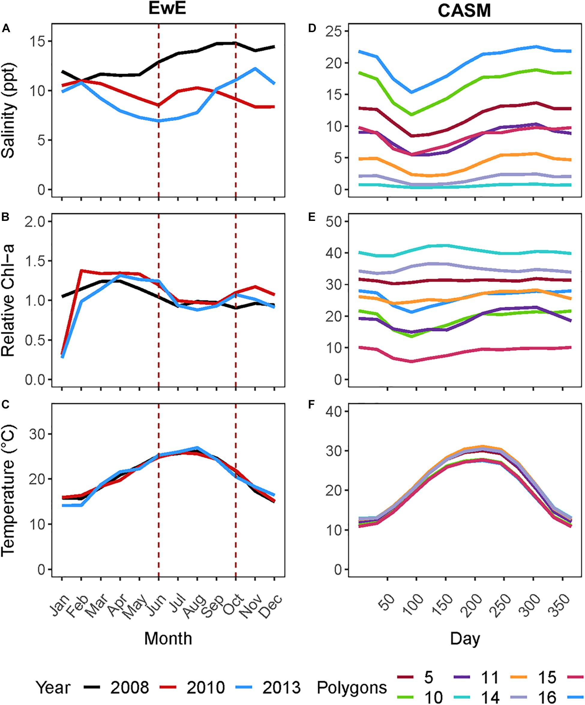
Figure 1. (A) Monthly salinity, (B) Chlorophyll-a concentration (μg l^–1), and (C) temperature for the three years from which rebalanced EwE time slices were extracted. (D) Climatological daily salinity, (E) Chlorophyll-a concentration (μg l^–1), and (F) temperature for eight CASM polygons used as input to the calibration simulations.

FIGURE 2

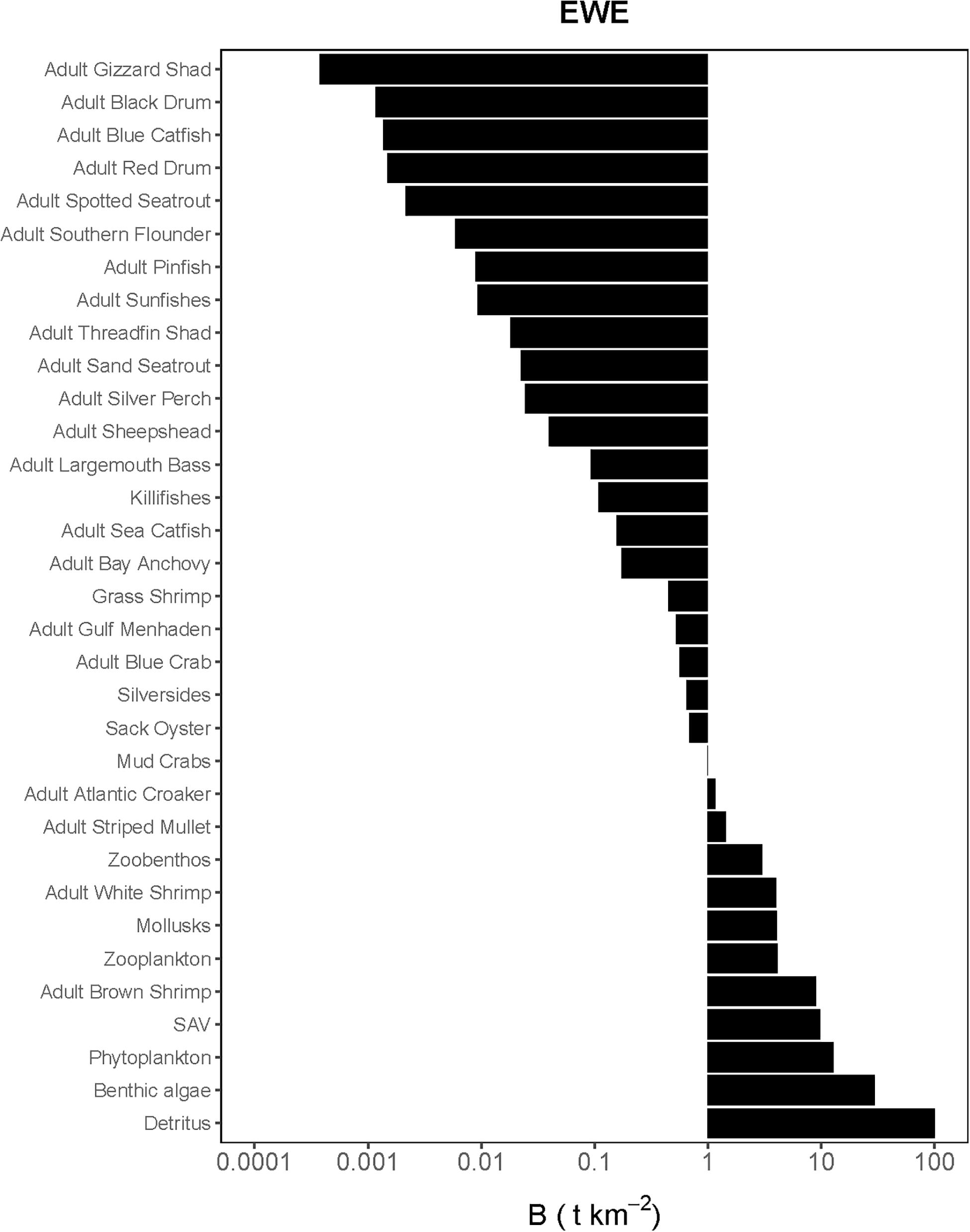
Figure 2. Species-biomass distribution of the Ecopath base model used in the calibration simulation of Ecosim (plotted on log scale). EwE plot is only displaying adult life stages as biomasses for juveniles were calculated using von Bertalanffy (1933) growth model.

FIGURE 3

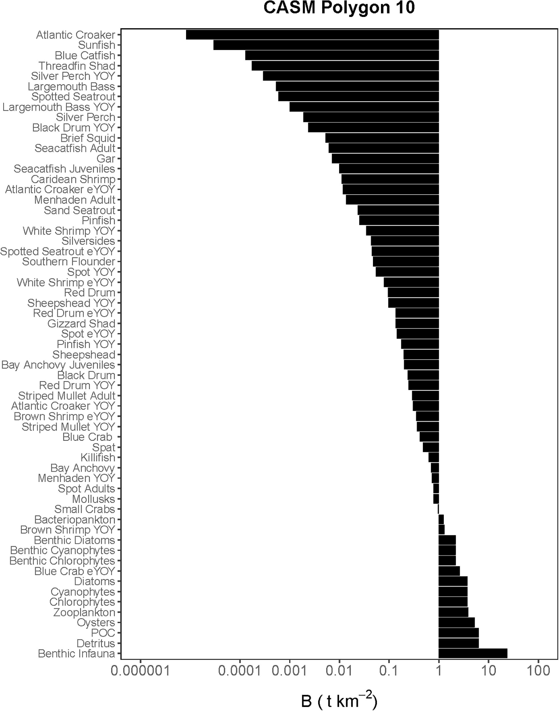
Figure 3. Comprehensive aquatic systems model (CASM) species-biomass distribution for June 15 in polygon 10 (plotted on log scale).

Prior to beginning the analysis for the current study, we first considered the degree of agreement between predicted and observed values of species biomasses over time from each calibrated simulation. Agreement was generally high for both models in their respective calibration simulations (Figure 4). The Ecosim simulation generally captured the mean and variation in the annual observed data for the key species groups (Figures 4A–E, see Table 1 in De Mutsert et al., 2017). The fit statistics showed variable but generally acceptable correlation (overall average r = 0.4) and low percent bias (average = 22%) across species groups. The CASM daily predicted biomasses of the key species groups (averaged over polygons) also showed an adequate fit to the observed biomasses well (Figure 4B); the fit statistics showed variable but generally high correlation (overall average r = 0.4, with 50% of species having a r > 0.6) and low percent bias (average = ± 30% for moderate to high biomass species) across species groups (see Table 5 in Dynamic Solutions, 2016).

FIGURE 4

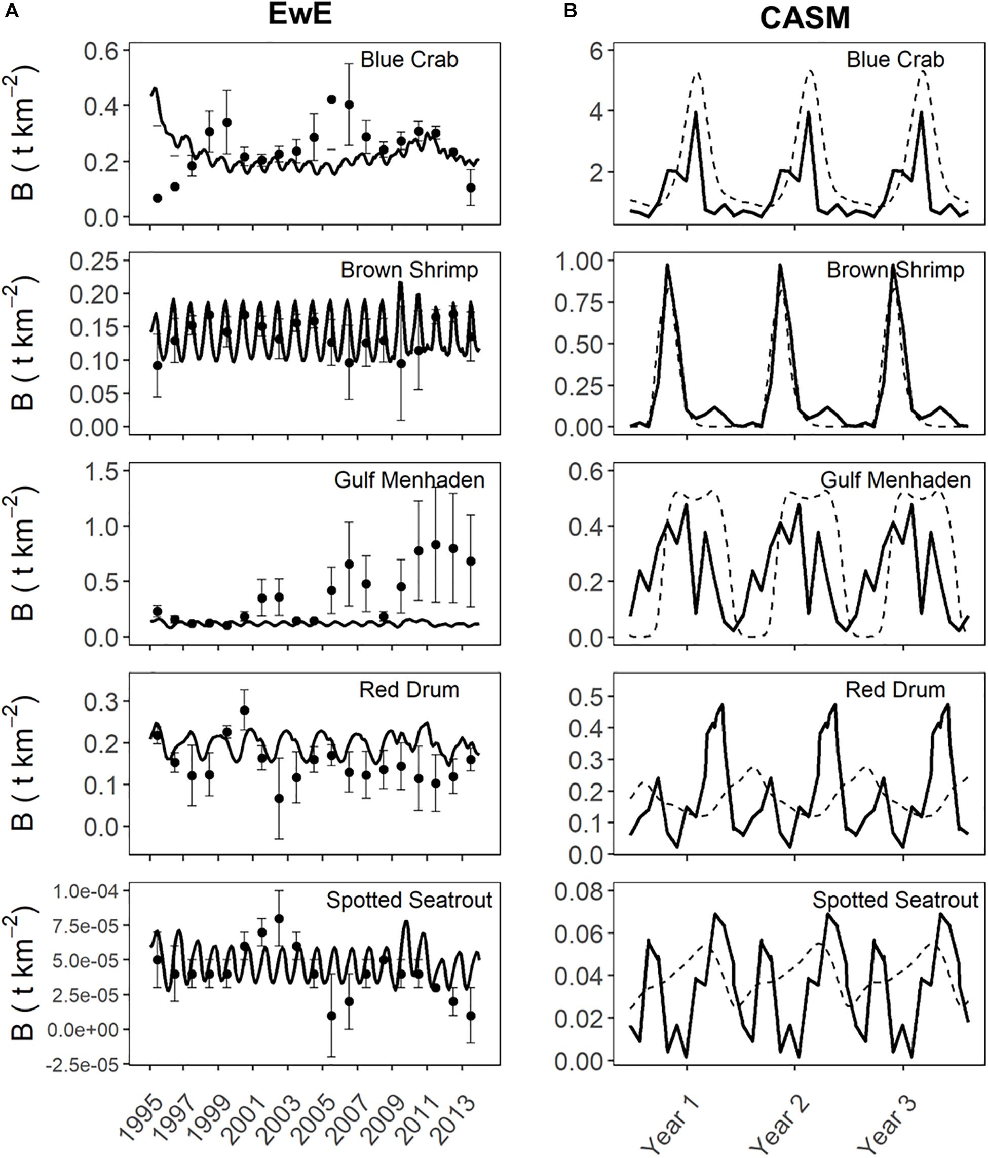
Figure 4. Predicted versus observed biomasses over time from selected species represented in both the Ecosim (A) and CASM (B) calibration simulations. Observed biomasses were annual for Ecosim and daily for CASM. Both used the same monitoring data that was monthly, which were averaged for Ecosim and interpolated for CASM. Ecosim predictions were for the entire model domain, while CASM predicts were averaged over the polygons comprising the domain of the Barataria Bay.

For this coordinated analyses, which used both models, we applied the results of the EwE calibrated model (Ecosim) for June and October of 2008, 2010, and 2013 (i.e., six food webs or balanced Ecopath models). These years were selected because the physical-biological model (Delft3D) used to provide driving variables (e.g., salinity, Figure 1A) to the EwE model (Baustian et al., 2018) reflected different hydrographic conditions in the time periods up to and including each of these years. June within each year is a period of relatively high productivity reflecting the results of the spring increased river flow and coincides to the month near the end of the operations of the proposed project. October is a period of relatively low biological productivity, as it occurs during a period of low river input and cooling temperatures. The year 2008 can be considered to have relatively high salinity and low chlorophyll-a concentrations in June and October compared to the same months in years 2010 and 2013 (Figure 1A). We used specific years from the Ecosim simulation to ensure realism because environmental conditions covary (typically through river flow) together in model inputs; however, this fact also shows that differences among years in environmental conditions are not simply different in a single factor such as temperature or salinity.

To create the balanced food web models from the calibrated Ecosim model, a plug-in to Ecosim was developed that generated Ecopath models from these six chosen time periods. The plug-in ran the Ecosim model up to a chosen month and year in the calibration simulation and then output all parameters from that snapshot in time (i.e., a time slice). For each time slice of Ecosim (June and October of three separate years), a rebalanced Ecopath model (a static snapshot of the ecosystem) was created so that the ecological indicators could be generated. The rebalancing involved adjustments to species-specific biomass accumulation rates in each Ecosim slice. Because the biomass accumulation rates just indicate the change in biomass from the base model to the time slice, the adjustments did not affect the biomasses, diets, or turnover rates within each time period. In addition, the adjustments, when needed, were generally small in magnitude. Thus, the rebalancing did not affect the calculations of the indicators outputted from the Ecopath Network Analysis Plug-in (Christensen and Pauly, 1992) used in this study.

The analysis of the calibrated CASM simulations used here were the daily output for each of eight polygons within the Barataria Bay (Figure 5, polygons 5, 10, 11, 14, 15, 16, 17, and 19). Because the environmental conditions were climatological (i.e., averaged by day across years), a single year of daily output was used from the sequence of repeated identical years in the calibration simulation. The eight polygons were selected to provide a range of environmental conditions, with a particular focus on salinity and chlorophyll-a concentrations (Figures 1D–F). Figure 6 shows the range of the average annual values of salinity and chlorophyll-a concentrations of the eight selected polygons. Use of multiple polygons allowed calculation of indicators for various combinations of salinity and chlorophyll (productivity) conditions within the Bay: (1) low salinity with high chlorophyll (polygons 15, 16, and 17); (2) intermediate salinity with low chlorophyll (polygon 19), with intermediate chlorophyll (polygon 14) and with high chlorophyll (polygon 10); and (3) high salinity with intermediate chlorophyll (polygons 5 and 11).

FIGURE 5

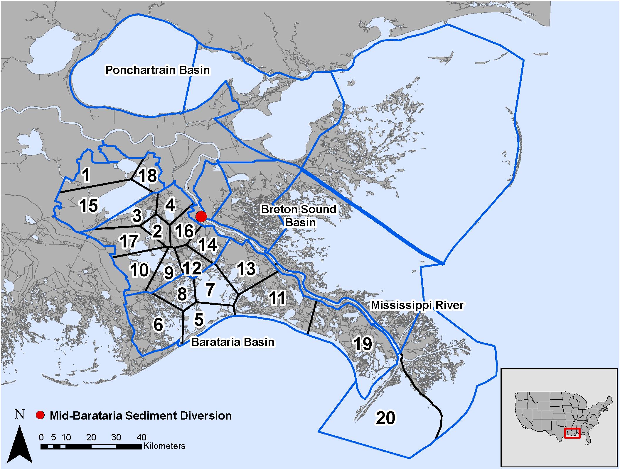
Figure 5. Model domain in the Mississippi River Delta, United States for the EwE (outlined in blue) and CASM (numbered polygons) calibrated simulations and location of the Mid-Barataria Sediment Diversion (red point).

FIGURE 6

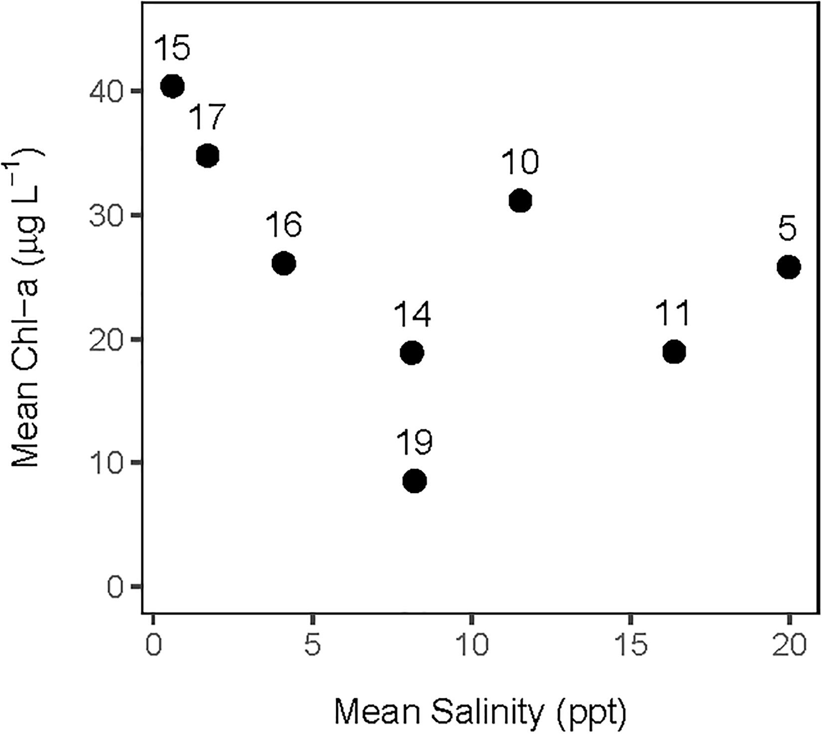
Figure 6. Averaged annual values of daily salinity and chlorophyll-a concentration for each of the 8 polygons used in this analysis of the CASM calibration simulation.

Selection and Interpretation of Indicators

We determined during a series of modeling team workshops that point-by-point comparisons of species group biomasses between the two models was not informative for assessing responses to disturbances. The strength of combining the results from the two models was in their prediction of higher-order indicators of food web structure and energetics. By using a standardized set of indicators, results from both models would provide a robust view of the food web in Barataria Bay and provide a basis for projecting how the food web would respond to disturbances. When taken together and consistently calculated from both models, judicious selection of these higher-order indicators would provide information on community structure, the connectivity of the food web (which species are connected to other species), and how fast and efficiently energy flows from the primary producers and detritus up through the food web via different pathways of connected species. Inclusion of certain indicators would also provide qualitative information on high-order food web properties, such as general energetic activity and resilience (Christian et al., 2010; Canning and Death, 2018).

There are dozens of candidate indicators that could be used to help inform natural resource managers (Borrett, 2013; Fath et al., 2019; Safi et al., 2019). During our modeling team workshops, we strategically selected indicators that covered the major features of the food web, were suggested by the literature, and for which both models produce the output needed for their calculation (Table 1). The details of how the indicators are calculated from model outputs are described elsewhere (e.g., Ulanowicz and Norden, 1990; Christensen et al., 2005; Heymans et al., 2016). Our focus is on their interpretation within and across models. The selected suite of indicators can be grouped into categories based on what features of the food web they help to describe.

TABLE 1

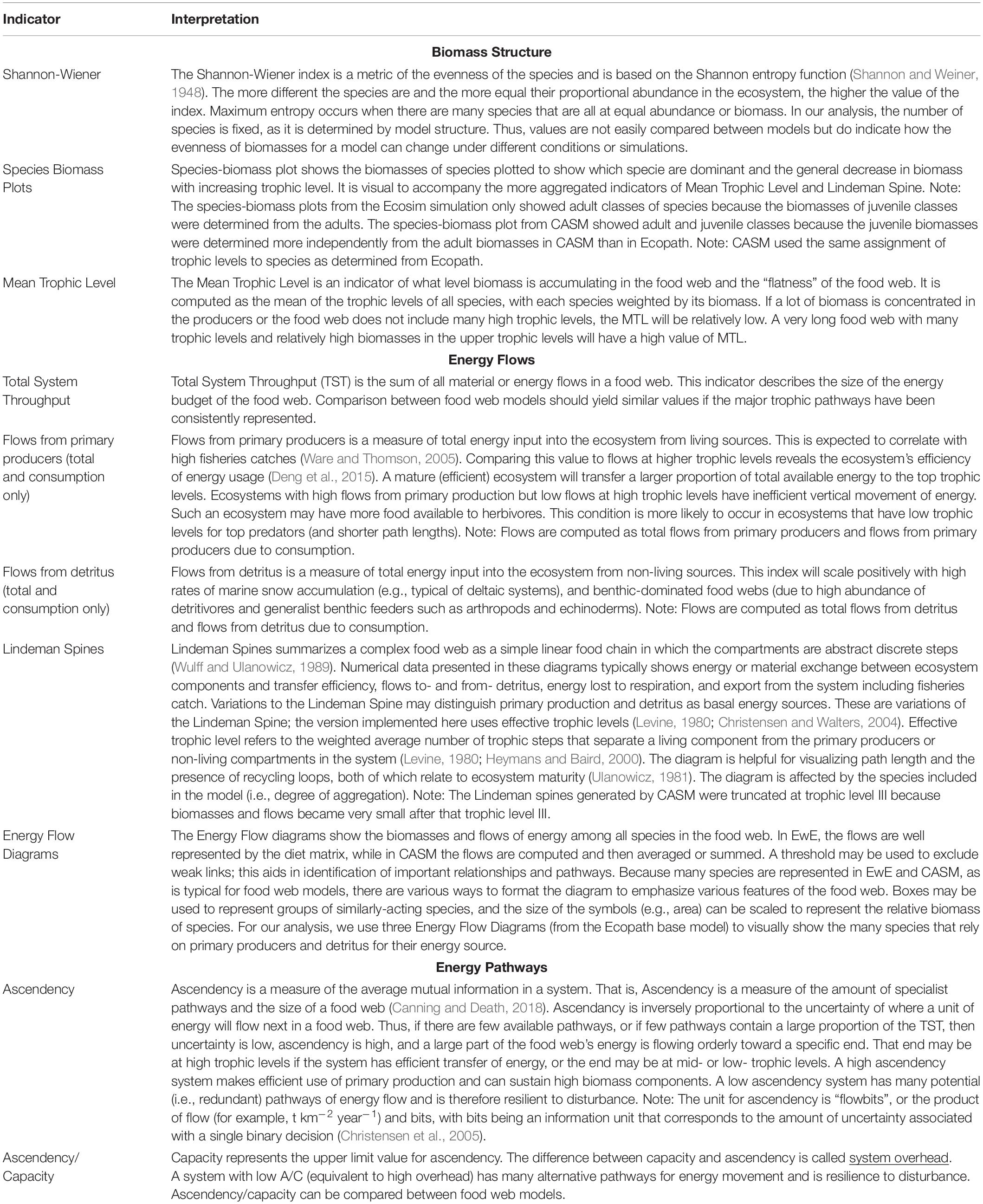
Table 1. The indicators and their interpretation derived from the calibration simulations of Ecopath and CASM for the Barataria Bay.

The first set of indicators (Shannon-Wiener Index, Species-biomass plots, and Mean Trophic Level Index) summarize the biomass structure of all species in the simulated food webs (Table 1). Since the list of species between time or space snapshots does not vary (i.e., species groups are fixed in both models), changes in our Shannon-Wiener values between snapshots (Ecopath and CASM) indicate differences in the evenness of the biomass distributions across all species. The mean trophic level index is a biomass-weighted average of the trophic levels across species.

The second group of indicators focuses on how energy flows among the species within the food web (Table 1). Using the Ecopath base model, we illustrated how energy flows up the food web with ecological flow diagrams that show the energy paths from three producer groups (pelagic algae, benthic algae, and detritus) to consumer species (see example in Figure 7). Both models are used to summarize energy flows with additional indicators: (1) comparison of the sum of all energy flows from primary producers versus the sum of all energy flows from detritus, (2) comparison of the summed energy flows from primary producers to consumers versus summed energy flows from detritus to consumers (3) total system throughput (TST), and (4) reduction of the food web into a simple linear food chain through a Lindeman Spine diagram. The first and second indicators in this group characterize the importance of detritus as an energy source to the food web relative to primary production; the second indicator specifically characterizes the importance of detritus and primary producers to consumers (i.e., detritivory). Total system throughput is the sum of all energy flows in the food web and is a measure of the energy budget. The Lindeman spine summarizes the food web by using the full food web information to estimate the equivalent linear food chain.

FIGURE 7

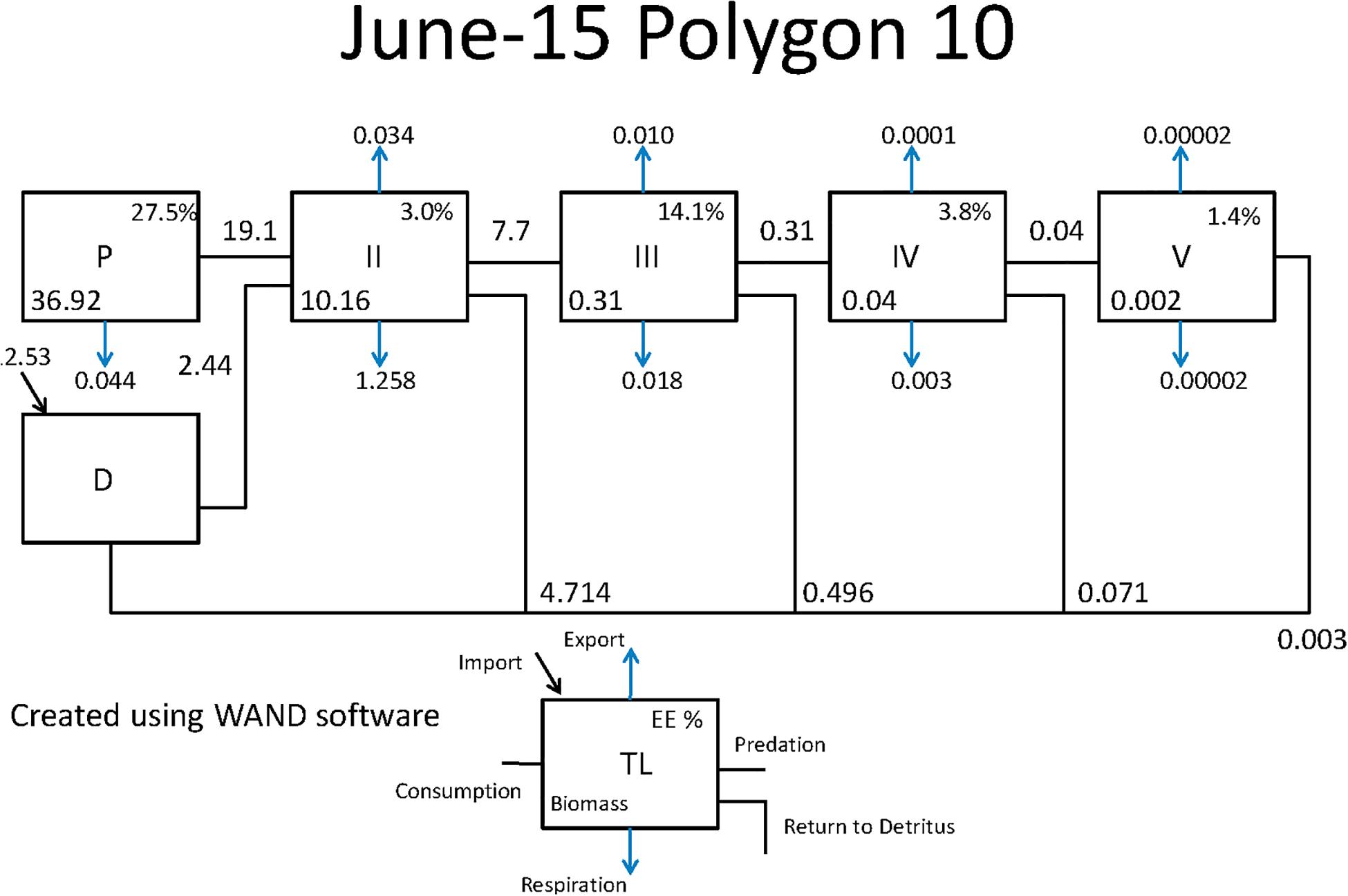
Figure 7. Example Lindeman Spine diagrams from the CASM model for polygon 10 on June 15. Biomasses are t km^–2 and flows are in t km^–2 day^–1 (Allesina and Bondavalli, 2004).

The third and final group of indicators derived from Information Theory (Ulanowicz, 1997) provides further insights into the energy pathways by quantifying the dominance and complexity of the pathways of how energy flows up the food web and provides a measure of the resilience of the food web (Table 1). These indicators are related to each other and are termed: ascendency, capacity, the ratio of ascendency to capacity (A/C), and overhead. Ascendency measures the efficiency of the pathways used by energy as it flows up the food web; high ascendency indicates that the food web makes efficient use of primary production and can sustain high biomass. High ascendancy usually implies a less disturbed system that is also less resilient to future disturbances (Ulanowicz, 1997). Capacity is the maximum value possible for ascendency. The difference between capacity and ascendency is system overhead. Overhead measures the complexity, where high overhead is indicative of a system that has many alternate pathways for energy movement and is therefore relatively more resilient, within certain bounds, to disturbance. The ratio of ascendency to capacity (A/C) is useful for indicating resiliency (where a low A/C is indicative of a highly resilient system) and the ratio is comparable across models and food webs. Overhead is calculated as 1- A/C and so varies in the opposite direction as A/C (Ulanowicz, 1997; Canning and Death, 2018).

Generation of Indicators

All indicators were computed from the rebalanced Ecopath models (derived from the calibrated Ecosim time slices) using the Ecological Network Analysis Plugin and from the output of the CASM calibration simulation. Thus, there were indicator values for six Ecopath food web snapshots (June and October from 2008, 2010, and 2013) and indicator values for eight food web snapshots (different polygons under climatological conditions) from CASM.

Results

The suite of indicator values showed consistent similarities and differences within each model and between models (Tables 2, 3) that, when combined, provided a description of the seasonal, interannual, and spatial variation in food web structure and energetics of Barataria Bay. The ecosystem indicators generated by both models showed the models were sensitive to changes in environmental conditions. The average Shannon Weiner index for Ecopath in June was 2.01 and 1.99 in October. For CASM, average Shannon Weiner indices were grouped by environmental conditions (Table 2) and were 3.00 (polygons 5, 11), 2.95 (polygons 10, 14, 19) and 3.16 (polygons 15, 16, 17), respectively. The mean trophic level across both models was ∼2, except for polygons 15 and 16 for CASM, which reported a mean trophic level of 3. Total system throughput (TST) was on average higher in all June years compared to October years in Ecopath (Table 3). CASM reported more variable TST across grouped polygons, with the highest value of 5372 t km^–1yr^–1 reported in polygon 10. Productivity and flows from detritus metrics were generally higher for all June years in Ecopath and for polygons 10, 15, 16, and 17 (Tables 2, 3). Ascendency metrics in Ecopath are highest in all June years compared to the October years. In CASM, ascendency/capacity remains constant over all time periods, while ascendency alone shows a range of values from 1798 flowbits to 6498 flowbits over all polygons. As the final step in our modeling team workshops, participants interpreted the model results together with the goal of using the indicators to formulate four general findings that would provide a basis for projecting how the food web would respond to disturbances and the proposed sediment diversion. The findings used both similarities and differences in the indicators between the two models and leveraged their structural and implementation differences (e.g., Ecopath for seasonal dynamics and CASM for spatial dynamics).

TABLE 2

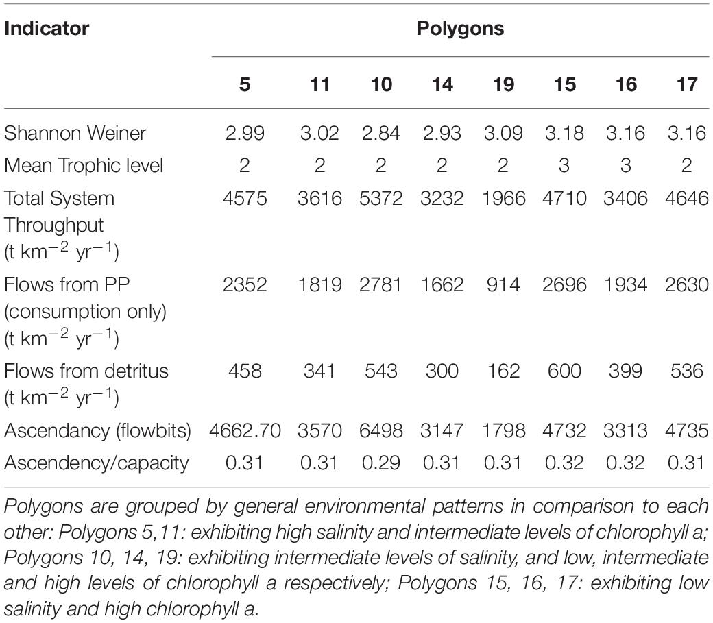
Table 2. Indicator values from the eight spatial polygons for the calibration simulation of CASM.

TABLE 3

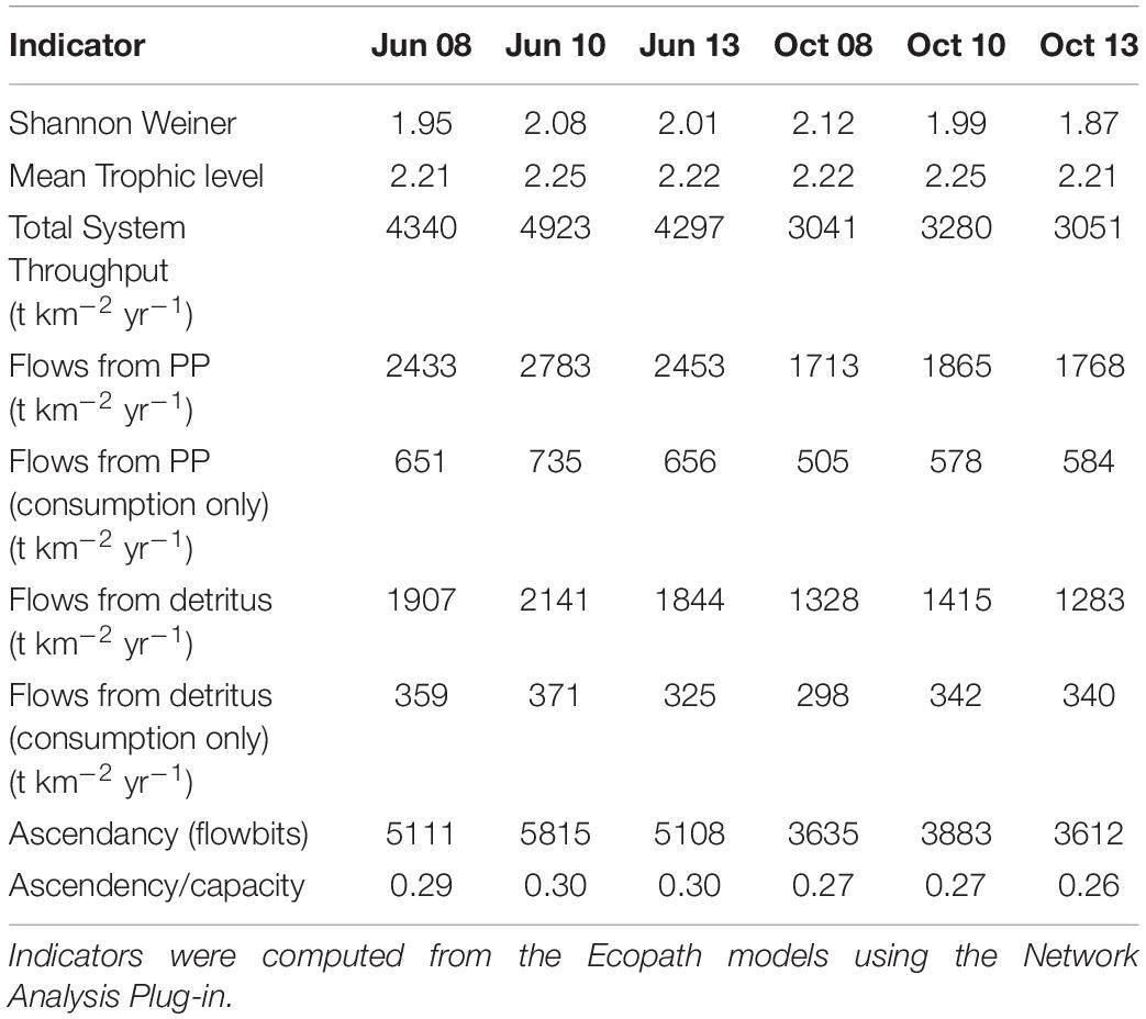
Table 3. Indicator values from the Ecopath food web snapshots taken from the calibration simulation of Ecosim.

Key Finding 1: Detritus Plays an Important Role in the Energetics and Functioning of the Barataria Food Web

A substantial store of decomposing material sustains high levels of detritivory in the simulated Barataria Bay food web and was responsible for a sizable fraction of the total energy budget in the food web. CASM outputs indicated that detritivory accounted for approximately 10.4% of all flows present in the food web (i.e., calculated as flows from detritus to consumers/total system throughput; Table 2). For comparison, 53% of the flows were herbivory (flows from primary producers to consumers/total system throughput). Herbivory and detritivory together accounted for all new energy inputs to the system. Thus, flows from detritus accounted for (10.4/(10.4 + 53)^∗100) = 16% of all energy input to the food web. This value is based on averaged annual flows over the eight polygons; the result is robust because the contribution of detritus relative to primary production was similar among polygons (range from 15% to 18%). Ecopath output indicated an even more important contribution from detritus: detritivory accounted for 35% of flows in the food web and primary consumption accounted for 65%. Flows from PP (consumption only) averaged 618 t km^–2 yr^–1 and flows from detritus (consumption only) averaged 339 t km^–2 yr^–1 (Table 3). Thus, flows from detritus accounted for (339/(339 + 618)^∗100) = 35% of all energy input to the system, and flows from PP accounted for (618/(339 + 618)^∗100) = 65%. Similar to the spatial consistency in CASM, the contribution of detritus relative to primary production was similar among the six Ecopath slices (33% to 37%). Thus, both models indicated a large (16% and 35%) portion of all energy into the food web was detrital, and this large contribution occurred when productivity was low and high (May and October in Ecopath) and uniformly within the bay (polygons in CASM).

Both CASM and Ecopath results also indicated a net production of new detritus in the system. The total annual flow into detritus pools from summed daily allochthonous inputs, and from daily mortality and excretion of producer and consumer groups for CASM was computed by polygon and then averaged over the eight polygons. The flow into detritus was equal to 670 t km^–2 y^–1, while the averaged flow out from the detritus biomass pools (Table 2) due to consumption was lower at 417 t km^–2 y^–1. A daily snapshot Lindemann Spine from a single polygon in CASM (Figure 7) further illustrated the high net production rates of detritus (12.53 versus about 8 t km^–2 d^–1 exiting). Our illustrative Ecopath slice shows flows from consumers into detritus of 396 t km^–2 and flows out of detritus due to consumption at 346 t km^–2 (Figure 8). The higher inflow in both the CASM and Ecopath models shows a detritus surplus because it was created faster than it was consumed. Ecopath energy flow diagrams provided additional evidence of the role of detritus, as many species were receiving energy originating from phytoplankton, phytobenthos, and detritus. The cumulative effect of these many linkages was the large energy fluxes emanating from the detritus pool (Figure 9).

FIGURE 8

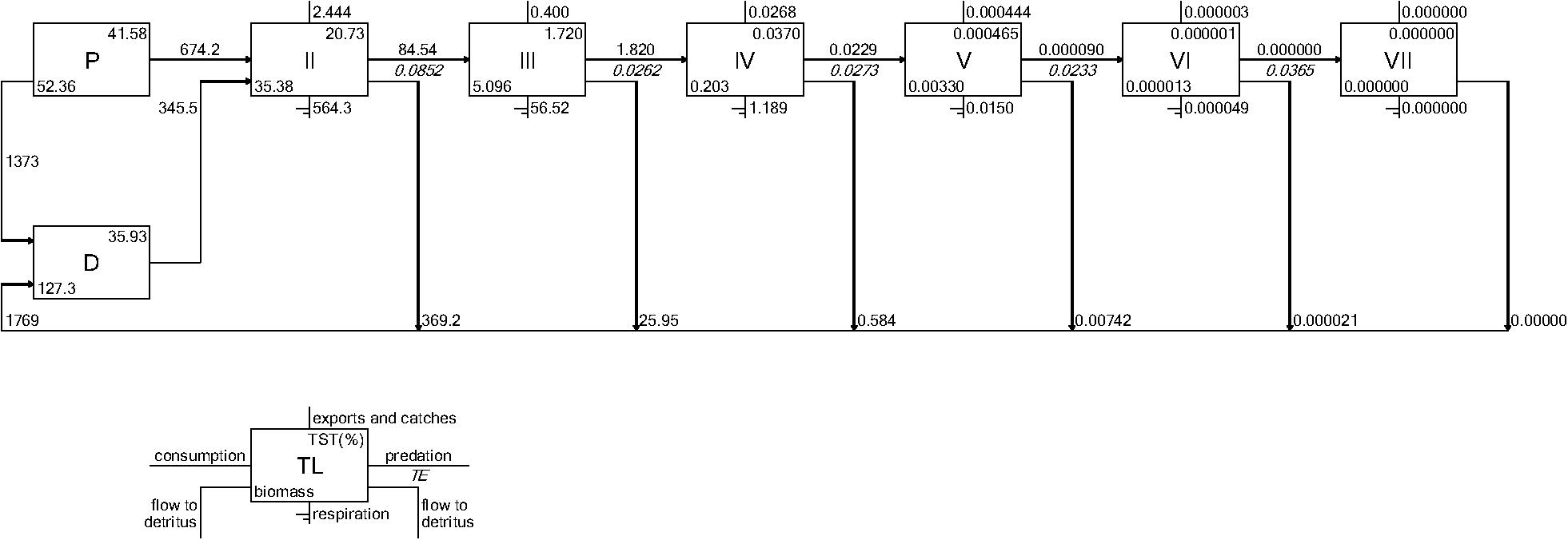
Figure 8. Example Lindeman Spine diagrams from the June 2010 Ecopath model determined from time slices from the Ecosim calibration simulation. Biomasses are in t km^–2 and flows are in t km^–2year^–1.

FIGURE 9

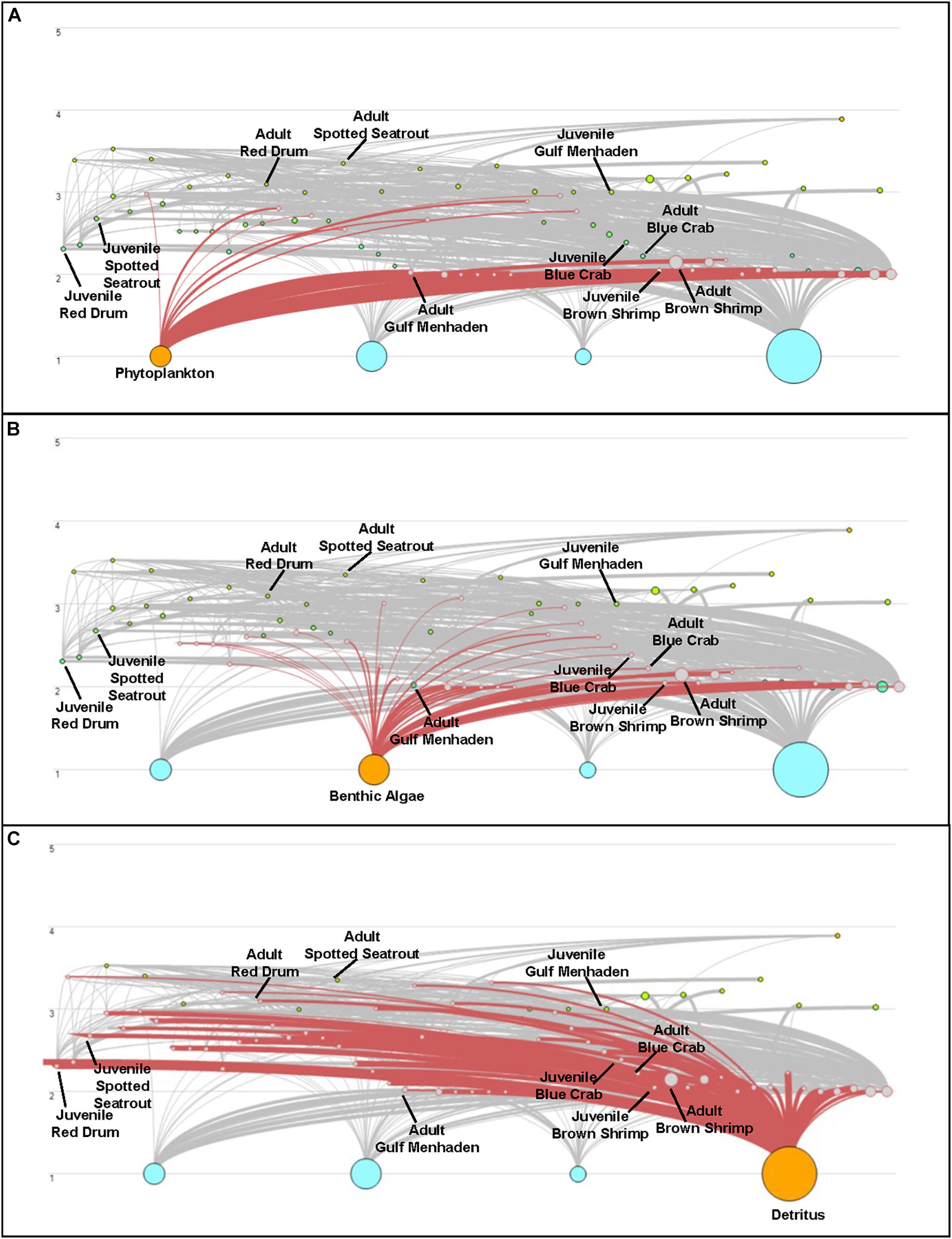
Figure 9. Energy Flow diagrams from the Ecopath base model used in the Ecosim calibration simulation to highlight net production of detritus in the model compared to other producer compartments. Trophic level is indicated on the y-axis; the size of the dots indicates the size of the biomass pools. Energy flow (t km^–2 yr^–1) from phytoplankton (A), Benthic Algae (B), and Detritus (C) is highlighted. This figure represents the key species found in both the CASM and EwE models.

Key Finding 2: The Barataria Bay Food Web Shows a Response of Increased Productivity After the Spring High Flow Season That Is Mediated Through Specific, Dominant Pathways

Seasonally representative output from the Ecopath food webs indicated a greater total system throughput in June compared to October. The average June value (over years) compared to October was 4,520 versus 3,124 t km^–2y^–1 (Table 3). Not only was the TST higher in June than in October, but ascendency (averaged over years) was also higher [5,345 versus 3,710 flowbits (t km^–2y^–1*bit)]. The mean trophic level of the food web (computed starting with consumers at trophic level 2) did not vary much with this seasonal (October versus June) increase in biomass, suggesting that the biomass increase occurred in species with a trophic level near 2.2. CASM-generated TST and ascendancy were highest in polygons 15, 17, 10, and 5 (Table 2), which are the polygons with the higher primary production/bottom-up food web support (Figure 6). The lowest TST and ascendancy values were in the polygons with the lower primary production. The magnitudes in the TST and ascendancy of the polygons generally tracked the chlorophyll-a (index of productivity) in the polygons (Table 2 and Figure 6). Therefore, the spatially explicit CASM results, when viewed temporally (space-for-time), represent a temporal pattern that is consistent with the Ecopath prediction of increased productivity after the spring high flow season.

Key Finding 3: The Trophic Pyramid of the Barataria Food Web Is Truncated

The Lindeman spines estimated from the Ecopath and CASM food webs indicated a large decrease in the amount of biomass above trophic level 2 (examples of selected spines shown in Figures 7, 8). This pattern was consistent for June and October for all three years from Ecopath, and on an annual basis for the eight polygons from CASM. The drop off can be easily visualized by the species-biomass distribution plots, which showed a decrease in biomass moving up the trophic levels (bottom to top in the plots) even when biomasses are plotted on a logarithmic scale (Figures 2, 3). The relatively low mean trophic level of the food web indicated by both models is commensurate with a truncated trophic pyramid structure (CASM: 2.33 to 2.51 across polygons; Ecopath: 2.21 to 2.25 seasonally).

Key Finding 4: Compared to Other Estuaries, the Barataria Bay Food Web Has Many Potential Pathways for Energy Transfer

The relatively low ascendency/capacity (A/C) ratio from both Ecopath (Table 3) and CASM (Table 2) indicated low predictability of energy flows within the food web. Both models indicated there were many potential pathways for a unit of energy to travel, that is, flow from producers to consumers is less predictable. That is, there is a large number of species found in first and second order consumers and this energy moves up the food web through these various pathways. The overall averaged A/C from Ecopath (28%) and CASM (31%) food webs were both considerably lower than A/C values reported for other estuarine food webs (e.g., Christian et al., 2005).

Discussion

Use of multiple ecosystem and food web models to inform natural resource management decisions are increasing (e.g., Peterman, 2004; Link et al., 2012; Townsend et al., 2014). Our analysis of two alternative food web models for Barataria Bay provided baseline information to help guide management decision-making on a large-scale restoration project. The goal was to identify how the food web might respond to changing estuarine conditions by providing a fundamental understanding structure and functioning of the system. The complementary use of the Ecopath and CASM models, leveraging their respective strengths, provided a robust view of the food web and its general responsiveness to disturbances. This collective approach was achieved by forming a team that included the expert panel of scientists and model developers, with periodic check-ins with the state and federal managers, who worked collaboratively to synthesize model results. The results presented here were provided to the management agencies charged with evaluating the potential impacts of the project. Further analyses could involve systematically perturbing the food webs in a generalized manner (e.g., altered growth rates) in both models to mimic anticipated changes in water quality from project operations.

Using multiple models provides several advantages when considering the use of model output in natural resource management decisions. The ecosystem indicators calculated provide only one value per ecosystem snapshot. Multiple models can provide for ‘samples’ of ecosystem function indicators. This ability to sample indicators is especially important to evaluate if the representations of the ecosystem are different under different environmental conditions. For example, seeing higher ascendency values for both models under higher productivity scenarios allows us to interpret a link between productivity and ascendency. The differences in model structure also provides a way to describe the food web under alternate views of how the species and environmental variables interact.

While this case study is based on one geographic location and restoration action, the methodologies used herein can be broadly applied. The long-term collaboration between scientists, agencies and managers started during the initial scoping phase of this project and continued throughout the application phase (Beier et al., 2017; Laudien et al., 2019), making this approach particularly compelling. This extended working relationship lays a solid foundation for future applications of using co-production in natural resource management decisions. The rapport built between the government agencies and modeling teams helped guide the science as results were collectively discussed during workshops and conference call check-ins. Co-production using action science methodologies is gaining traction across the world (Gross and Hagy, 2017; Laudien et al., 2019) and successful projects like this one make the case for continued expansion of these practices. Therefore, we contend this approach to using multiple models for natural resource decision-making can be applicable in other contexts and ecosystems.

Implications of Key Findings for Decision-Makers

Our analysis of the indicators provided baseline information on the structure and energetics of the Barataria Bay food web and can be used to infer how the food web would respond to disturbances (or changes in environmental conditions caused by sediment diversions). Collectively interpreting the average range of flows from detritus of 16% to 35% (Tables 2, 3), suggested that detritus played a significant role in supporting fish and fisheries in Barataria Bay and that the food web has multiple pathways of moving fresh (chlorophyll) and recycled (detritus) organic matter into the food web. Such influence of detritus is typical of shallow deltaic systems with high rates of production and deposition (Odum, 1984; Kennish, 1990). Because a large part of the food web’s total energy budget derives from the breakdown of detritus, the modeling results indicated that there exists a short-term energy reserve in the system that is somewhat independent of primary production and therefore insensitive to light limitation and other factors that may limit primary production. This property suggests some potential uniformity in the production rate of detritivorous species and their predators during short-term increases in system turbidity or other disturbances that may limit phytobenthos or phytoplankton production. Fisheries targeting detritivorous species, such as shrimp and blue crab, may benefit from this buffering effect.

Also noteworthy from the indicators was that the detritus-based food web supported a different array of species than either the phytoplankton or phytobenthos-based food webs (Figure 9). Long-term changes in detrital inputs, composition, or dynamics can therefore result in a shift in species composition and changes in the structure of the food web (De Mutsert and Cowan, 2012). Reliance on the detrital dynamics has been shown to offer enhanced ecosystem stability (Moore et al., 2004). In particular, the extent to which detritus is delivered by freshwater sources or adjacent marshes (i.e., allochthonous sources) versus produced by the decay of phytoplankton and phytobenthos (i.e., autochthonous sources), which can be affected by disturbances, will also modulate the food web structure and energetics.

Seasonal inputs from rivers are important to the normal functioning of the food web in many estuaries as they stimulate primary and secondary production in the spring and summer (Madden et al., 1988; Nielsen et al., 2004; Cloern et al., 2014). These inputs fuel seasonal increases in dominant-biomass low-trophic level species (e.g., phytoplankton, benthic algae). These species groups serve an important ecological role as they facilitate energy transfer to higher trophic levels. The Ecopath slices indicated higher throughput in June for Barataria Bay that reflected the tail end of the spring bloom and suggests that high biomass and consumption rates were concomitant with an increase in primary productivity (TST is positively related to chlorophyll-a concentration in both models). The truncated nature of the food web indicated in the Lindeman spines (Figures 7, 8) show that the seasonal peak in biomass (June versus October) is concentrated in a large number of species found at lower trophic levels (i.e., TL < 3). Environmental changes, or changes in the supply of nutrients, could therefore alter the seasonal production of these high biomass, low trophic level consumer groups, such as shrimp, anchovy, and menhaden.

Indicators also showed that most of the biomass within the food web was organized at lower trophic levels, and because low-trophic level species have high turnover rates, there is potential for high population growth rates over short periods of time (e.g., 1–2 years). Such turnover provides a mechanism for these species to be relatively resilient to short-term disturbances. Changes to environmental conditions can have large effects on the food web because environmental conditions influence the base of the food web, and a large portion of food web biomass is found in basal and lower-trophic level species (Odum, 1971, e.g., phytoplankton, zooplankton, and forage species). Due to this strong and direct connection between the environment and biomass-dominant groups, the food web is liable to be variable and spatiotemporally responsive to changes in environmental conditions.

The truncated food web from both models indicated that average trophic pathways are short, and that predatory fish population production is unlikely to be limited by their consumption effects on their available food. Predator populations were kept low in simulations in part because of the assumed high rates of fishing mortality (e.g., in Ecopath - Fishing/Total (F/Z) mortality was 68% for menhaden, 81% for gray snapper, 45% for largemouth bass, and 27% for black drum) and other sources of removals (e.g., migrations in CASM). High rates of predation mortality by adults on juvenile fish might also contribute to relatively low levels of high trophic consumer biomasses. Short trophic pathways and an absence of substantial predator biomass both suggest that the system is donor (bottom-up) controlled. Low ecotrophic efficiencies (EE) in the Ecopath models estimated from the Ecosim simulation for mid-trophic level forage species reinforced this finding, as it also indicates low predation rates from higher trophic level species relative to production of forage species. Additional support was provided by the vulnerabilities set during calibration of Ecosim that suggested that biomass dynamics of forage fish species are not strongly controlled by predation (i.e., top-down control is weak compared to bottom up effects).

When viewed in comparison to other estuarine ecosystems, our analyses indicated that Barataria Bay has a relatively high level of resiliency because of its relatively low values of A/C. Christian et al. (2005) compared the A/C values of 6 separate estuarine ecosystems (with a total of 17 seasonal values) that showed an averaged value of 43% (standard deviation of 0.05). The lower A/C ratios generated with Ecopath and CASM (Tables 2, 3) are indicative of large food webs with varied consumer diets that result in many possible energy pathways through the food web (Morris et al., 2005). Both models represented multiple lower trophic level consumer species that feed on a variety of prey types (detritus, benthic algae, benthic infauna, and epifauna), and both models represented the pelagic aspect of their food webs with multiple forage fish species such as bay anchovy, shads, silversides, and gulf menhaden feeding on phytoplankton and zooplankton in the water column. This opportunistic feeding, which is typical of estuarine species (Elliott et al., 2007), allows top and mid-level predators to switch to other prey items when environmental conditions become unfavorable for certain forage species, increasing the resilience of the food web as a whole. Thus, for Barataria Bay, there is a large number of possible destinations for an energy parcel, and lower overall certainty of the destination of energy into the upper trophic levels. Although high A/C systems make more efficient use of energy to produce biomass, low A/C systems tend to have more pathways through which energy may flow (Ulanowicz, 1997; Canning and Death, 2018). Low A/C systems are therefore robust to disturbance, as redundant pathways for energy flow exist in case any single node (species or groups of similar species) is disturbed. Redundant food web connections (i.e., multiple potential pathways for energy transfer) help reduce the danger of furthering food limitation of predators even if important prey groups are disturbed or eliminated by fisheries or disturbances. Perturbations that occur on a limited number of species and connections can potentially be absorbed by the food web.

Note that while the food web as a whole may be resilient, individual species or groups in the food web can still be affected (some being reduced), and that the degree of resiliency and responsiveness of individual species depends on the type (where it affects the food web and how), magnitude, duration, and repetitiveness of the disturbance (Ulanowicz, 2018). A disturbance that broadly affects many aspects of the bottom of the food web (phytoplankton, phytobenthos, and detritus), and does so with high intensity for an extended time period and repeats every year, can exceed the resilience provided by redundant food web connections. It follows that the Barataria food web can likely absorb a disturbance that affects only part of the bottom of the food web and especially if the disturbance has only small to moderate impacts that occur once or with sufficient time between impacts.

Context for Interpretation of Indicators

We focused on June versus October for Ecopath and spatial differences via different polygons in CASM. A more direct analysis of model output would have evaluated the same outputs between the models so their predictions could be directly interpreted. Our primary purpose here was not to compare the models to determine when and where the models agreed and disagreed. Our purpose was to use the two models to characterize the Barataria Bay food web and to focus on the model results with sufficiently high enough confidence to be used to understand the food web. In our use of the calibration simulations, we noted several examples where both models generated similar predictions and also situations when the two models differed in their predictions but for valid reasons related to their alternative views of the food web. For instance, the strength of CASM under calibration conditions was to examine spatial differences in the food web within Barataria Bay on an annual basis. The calibration of Ecosim used year-to-year variation in environmental inputs for a large spatial domain so its strength lay in examining seasonal (rather than spatial) differences. The aim, therefore, was to combine the results from the calibration simulations of two models to describe the food web, and we contend this integration is the strength of this approach. By using both models, we were able to make statements about the average food web structure and energetics and how it varied seasonally (June versus October) and spatially (among polygons).

An important caveat centers on how the two models represent species biomass removals from their domains. Both the Ecopath and CASM models focus on the dynamics within their domains and attempt to account for species removals. These removals can affect the structure and energetics of the simulated food webs. Ecopath includes fisheries harvest, which removes significant fractions of biomass of certain species, and CASM includes emigration and immigration (in and out of the domain) for species. This difference is important because indicators that show a high importance of bottom-up controls on the food web (environmental to lower trophic levels) are conditional on relatively low biomasses of higher trophic levels, which may be low due to removals. Therefore, a major change in removals that allows higher biomasses of certain species can affect the finding that the food web during calibration conditions was being controlled by environmental forcing acting at the lower part of the food web.

Careful interpretation of ecosystem models is needed because the same labels can be attached to environmental variables, parameters, and processes even though they are used differently within alternative models. An example is the difference in how respiration is represented in the two models used here. Respiration rates in CASM will be lower because its formulation has additional loss terms to respiration (e.g., excretion) that are included in one respiration term in Ecopath. Both formulations are valid but one must identify this difference and look carefully at the models when respiration losses are included as part of the calculation of indicators.

We did not focus on using the calibration simulations to determine how general or project-induced changes in salinity would affect the food webs. Both Ecopath and CASM included the effects of variation in salinity (feeding in Ecopath; growth rate in CASM) within their calibration simulations. However, simulations of specific salinity scenarios are likely uncertain due to the need to specify salinity effects on multiple processes of many species; such simulations are achievable with additional model development and analyses. We suggest that a next step would be to perform new simulations with the calibrated models that vary environmental conditions (low versus high flow years) in a systematic way so that responses of the food web can be attributed, in a cause-and-effect manner, to generalized types of disturbances (e.g., reduced growth) imposed on species in the models.

The outcomes of this work resulted from a series of workshops lead by an expert panel of ecological modelers. These scientists worked previously with the state and federal managers to develop the most relevant plan for use of the food web models to support the management decision. Other participants included the marine ecologists who developed the food web models and representatives of the state and federal management agencies. During the workshops it was collectively determined that the EwE model should focus on two key months and the analysis of the CASM simulation should focus on the spatial differences in annual output provided by the multiple, independently simulated polygons. During the workshop, all participants determined which ecological indicators could be calculated with both models or what indicators should be used specifically from one model or the other. This systematic determination of indicators that included periodic discussions with the government agency representatives, allowed for a broad description of the structure, status, and resilience of the Barataria food web under natural variability of environmental conditions in the area. This action science approach to management also ensured the results provided to the interested agencies were scientifically sound and included relevant information to evaluate the efficacy of the restoration project.

Finally, we offer a few more caveats. First, some of the indicators are sensitive to the specific structure of the models. We used indicators that were robust but if a third model was considered or major changes were made in the use of Ecoapth or CASM, then the indicators should be re-examined to confirm how best to compare them across models and for project scenarios. The indicators remain valid descriptors of the food web; what should be re-examined are the actual values of the indicators and how to assess differences over time and space and between models. Second, while physical habitat is included in both models, both models assumed no major changes in physical habitat during the calibration simulation time period. The focus was on food web interactions assuming stable physical habitat conditions. Habitat suitability modeling being done separately from these food web models will provide information on the effects of changing habitat.

While much more can be inferred about the food web from further analysis of these models, the calibration simulations provided a sound foundation for the food web structure and energetics. Such information provides a food web context for assessing possible impacts of the proposed project. The management agencies have also used habitat suitability index (HSI) models to evaluate species-specific spatiotemporal differences in habitat suitability (between 0 and 1) based on varying salinity, temperature, water depth, proportion marsh, and other factors, for key fisheries (e.g., shrimps, blue crab, spotted seatrout) and wildlife (e.g., ducks, alligators) species in Barataria Basin. The HSIs provided simpler formulaic models for evaluating the Mid-Barataria Sediment Diversion operational alternatives for determining potential species impacts. The HSIs are much less complex, with modeled results, sensitivity, and uncertainty much easier to communicate for assessment of single species. HSIs are commonly used for impacts analysis for environmental assessments for water resource and restoration projects (CPRA, 2017), but multispecies or food web models are much less common. Using the calibrated EwE and CASM to describe the existing food web structure and energetics in Barataria Basin under varying spatial and temporal environmental conditions offered an expanded understanding and explanation of potential ecosystem-level impacts beyond HSI analysis.

Conclusion

Careful evaluation and testing of ecosystem models enable understanding of their strengths and limitations. We demonstrated how combining the results from two alternative models (Ecopath and CASM) for Barataria Bay is a scientifically sound and practical approach for dealing with the complexities of food webs and how they respond to environmental variation, resource management actions, and disturbances. There are a wide range of ways multiple models can be used, from a high degree of coordination during model development to complete independence until the synthesis at the end. A key step in all multi-model approaches is to ensure that the modeling results are interpreted properly (Rose et al., 2015; Schuwirth et al., 2019). We attempted to address the interpretation issue by working with managers so that the results were presented a manner that, as much as possible, could inform decision-making. Most multiple model situations are somewhere between the extremes of complete versus no coordination and thus determining the confidence to assign to results when models agree or disagree is challenging. Our approach presented here offers a template for combining modeling results that leverages the strengths of the different models by focusing on higher-order indicators (rather than variable-by-variable comparisons) that have relatively high confidence and also are useful to management (Fu et al., 2019). A critical aspect of our approach was the coordination between model developers and outside scientists, with input from natural resource managers, all working together in a collaborative effort.

Data Availability Statement

The data analyzed in this study is subject to the following licenses/restrictions: The data used for this manuscript can be received upon request to the Louisiana Department of Wildlife and Fisheries and the Louisiana Coastal Protection and Restoration Authority. Model source code can be made available upon request, in addition to the input and output data used in both modeling frameworks. Requests to access these datasets should be directed to brian.lezina@la.gov.

Author Contributions

KM and KL developed the EwE model. SS developed the CASM model. KR, CA, DB, and HT provided expert consultation on combining and collectively interpreting model outputs. KL, KR, KM, SS, CA, DB, and HT wrote the manuscript. All authors contributed to the article and approved the submitted version.

Funding

This project was supported by the Louisiana Coastal Protection and Restoration Authority (CPRA) with funding from the Louisiana Trustee Implementation Group (LA TIG).

Conflict of Interest

SS was employed by the company Dynamic Solutions, LLC.

The remaining authors declare that the research was conducted in the absence of any commercial or financial relationships that could be construed as a potential conflict of interest.

Acknowledgments

We would like to acknowledge and thank the Louisiana Coastal Protection and Restoration Authority (CPRA) and the Louisiana Trustee Implementation Group (LA TIG) for the opportunity to help guide critical management decisions for restoration projects in coastal Louisiana. Their feedback and comments since the inception of this collaborative modeling effort have helped to develop an ensemble modeling approach that can inform future management actions. KM and KL would like to thank Joe Buszowski and Jeroen Steenbeek for their work on the EwE model, Robert R. Christian for his comments on an earlier draft of this paper, and Victoria Roberts for her assistance in figure development for the paper. SS would like to thank Katherine Watkins for her help in development of the CASM model. The entire authorship would like to than Ehab Meselhe and Melissa Baustian and the many other academic and agency representatives that contributed time and data to this work.

Supplementary Material

The Supplementary Material for this article can be found online at: https://www.frontiersin.org/articles/10.3389/fmars.2021.625790/full#supplementary-material

Footnotes

1. ^ http://sirs.agrocampus-ouest.fr/EcoBase/

References

Allesina, S., and Bondavalli, C. (2004). WAND: an ecological network analysis user-friendly tool. Environ. Model. Softw. 19, 337–340. doi: 10.1016/j.envsoft.2003.10.002

CrossRef Full Text | Google Scholar

Bartell, S. M. (2003). A framework for estimating ecological risks posed by nutrients and trace elements in the Patuxent River. Estuaries 26, 385–396. doi: 10.1007/bf02695975

CrossRef Full Text | Google Scholar

Bartell, S. M., Lefebvre, G., Kaminski, G., Carreau, M., and Campbell, K. R. (1999). An ecosystem model for assessing ecological risks in Quebec rivers, lakes, and reservoirs. Ecol. Model. 124, 43–67. doi: 10.1016/s0304-3800(99)00155-6

CrossRef Full Text | Google Scholar

Baustian, M. M., Meselhe, E., Jung, H., Sadid, K., Duke-Sylvester, S. M., Visser, J. M., et al. (2018). Development of an Integrated Biophysical Model to represent morphological and ecological processes in a changing deltaic and coastal ecosystem. Environ. Model. Softw. 109, 402–419. doi: 10.1016/j.envsoft.2018.05.019

CrossRef Full Text | Google Scholar

Beier, P., Hansen, L. J., Helbrecht, L., and Behar, D. (2017). A how-to guide for coproduction of actionable science. Conserv. Lett. 10, 288–296. doi: 10.1111/conl.12300

CrossRef Full Text | Google Scholar

Borrett, S. R. (2013). Throughflow centrality is a global indicator of the functional importance of species in ecosystems. Ecol. Indicators 32, 182–196. doi: 10.1016/j.ecolind.2013.03.014

CrossRef Full Text | Google Scholar

Brugnach, M., Dewulf, A., Pahl-Wostl, C., and Taillieu, T. (2008). Toward a relational concept of uncertainty: about knowing too little, knowing too differently, and accepting not to know. Ecol. Soc. 13:30.

Google Scholar

Canning, A. D., and Death, R. G. (2018). Relative ascendency predicts food web robustness. Ecol. Res. 33, 873–878. doi: 10.1007/s11284-018-1585-1

CrossRef Full Text | Google Scholar

Chagaris, D., Sagarese, S., Farmer, N., Mahmoudi, B., de Mutsert, K., VanderKooy, S., et al. (2019). Management challenges are opportunities for fisheries ecosystem models in the Gulf of Mexico. Mar. Policy 101, 1–7. doi: 10.1016/j.marpol.2018.11.033

CrossRef Full Text | Google Scholar

Christensen, V., Coll, M., Steenbeek, J., Buszowski, J., Chagaris, D., and Walters, C. J. (2014). Representing variable habitat quality in a spatial food web model. Ecosystems 17, 1397–1412. doi: 10.1007/s10021-014-9803-3

CrossRef Full Text | Google Scholar

Christensen, V., and Pauly, D. (1992). Ecopath II—a software for balancing steady-state ecosystem models and calculating network characteristics. Ecol. Model. 61, 169–185. doi: 10.1016/0304-3800(92)90016-8

CrossRef Full Text | Google Scholar

Christensen, V., Walters, C., and Pauly, D. (2005). Ecopath with Ecosim: A User’s Guide. Fisheries Centre. Vancouver: University of British Columbia, 154.

Google Scholar

Christensen, V., and Walters, C. J. (2004). Ecopath with Ecosim: methods, capabilities and limitations. Ecol. Model. 172, 109–139. doi: 10.1016/j.ecolmodel.2003.09.003

CrossRef Full Text | Google Scholar

Christian, R. R., Baird, D., Luczkovich, J., Johnson, J. C., Scharler, U. M., and Ulanowicz, R. E. (2005). “Role of network analysis in comparative ecosystem ecology of estuaries,” in Aquatic Food Webs: An Ecosystem Approach, eds A. Belgramo, U. M. Scharler, J. Dunne, and R. E. Ulanowicz (Oxford: Oxford University Press), 25–40. doi: 10.1093/acprof:oso/9780198564836.003.0004

CrossRef Full Text | Google Scholar

Christian, R. R., Voss, C., Bondavalli, C., Viaroli, P., Naldi, M., Tyler, A., et al. (2010). “Ecosystem health indexed through networks of nitrogen cycling,” in Coastal Lagoons: Critical Habitats of Environmental Change, ed. M. Kennish (Boca Raton, FL: CRC Press).

Google Scholar

Cloern, J., Foster, S., and Kleckner, A. E. (2014). Phytoplankton primary production in the world’s estuarine-coastal ecosystems. Biogeosciences 11, 2477–2501. doi: 10.5194/bg-11-2477-2014

CrossRef Full Text | Google Scholar

Collie, J. S., Botsford, L. W., Hastings, A., Kaplan, I. C., Largier, J. L., Livingston, P. A., et al. (2016). Ecosystem models for fisheries management: finding the sweet spot. Fish Fish. 17, 101–125. doi: 10.1111/faf.12093

CrossRef Full Text | Google Scholar

Cooke, S. J., Nguyen, V. M., Chapman, J. M., Reid, A. J., Landsman, S. J., Young, N., et al. (2020). Knowledge co-production: a pathway to effective fisheries management, conservation, and governance. Fisheries 46, 89–97. doi: 10.1002/fsh.10512

CrossRef Full Text | Google Scholar

Couvillion, B. R., Beck, H., Schoolmaster, D., and Fischer, M. (2017). Land Area Change in Coastal Louisiana (1932 to 2016). 2329-132X. North Pole, AK: US Geological Survey.

Google Scholar

CPRA (2017). Louisiana’s Comprehensive Master Plan for a Sustainable Coast. Baton Rouge, LA: Coastal Protection and Restoration Authority of Louisiana.

Google Scholar

Dahood, A., Klein, E. S., and Watters, G. M. (2020). Planning for success: leveraging two ecosystem models to support development of an Antarctic marine protected area. Mar. Policy 121:104109. doi: 10.1016/j.marpol.2020.104109

CrossRef Full Text | Google Scholar

De Mutsert, K., and Cowan, J. H. (2012). A before–after–control–impact analysis of the effects of a Mississippi river freshwater diversion on Estuarine Nekton in Louisiana, USA. Estuaries Coasts 35, 1237–1248. doi: 10.1007/s12237-012-9522-y

CrossRef Full Text | Google Scholar

De Mutsert, K., Cowan, J. H. Jr., and Walters, C. J. (2012). Using Ecopath with Ecosim to explore nekton community response to freshwater diversion into a Louisiana estuary. Mar. Coastal Fish. 4, 104–116. doi: 10.1080/19425120.2012.672366

CrossRef Full Text | Google Scholar

De Mutsert, K., Lewis, K., Milroy, S., Buszowski, J., and Steenbeek, J. (2017). Using ecosystem modeling to evaluate trade-offs in coastal management: effects of large-scale river diversions on fish and fisheries. Ecol. Model. 360, 14–26. doi: 10.1016/j.ecolmodel.2017.06.029

CrossRef Full Text | Google Scholar

De Mutsert, K., Lewis, K. A., Buszowski, J., Steenbeek, J., and Milroy, S. (2016). Delta Management Fish and Shellfish Ecosystem Model: Ecopath with Ecosim plus Ecospace model description. Prepared for Louisiana Coastal Protection and Restoration Authority under LCA Mississippi River Hydrodynamic and Delta Management Project. Baton Rouge, LA: Coastal Protection and Restoration Authority.

Google Scholar

DeAngelis, D., Bartell, S., and Brenkert, A. (1989). Effects of nutrient recycling and food-chain length on resilience. Am. Nat. 134, 778–805. doi: 10.1086/285011

CrossRef Full Text | Google Scholar

DeFries, R., and Nagendra, H. (2017). Ecosystem management as a wicked problem. Science 356, 265–270. doi: 10.1126/science.aal1950

PubMed Abstract | CrossRef Full Text | Google Scholar

Deng, L., Liu, S., Dong, S., An, N., Zhao, H., and Liu, Q. (2015). Application of Ecopath model on trophic interactions and energy flows of impounded Manwan reservoir ecosystem in Lancang River, southwest China. J. Freshw. Ecol. 30, 281–297.

Google Scholar

Dynamic Solutions (2012). Delta Ecological Model for Use in the Delta EFDC Hydrodynamic Model. Final Report Submitted to the Sacramento District, U.S. Army Corps of Engineers for the CalFed/Delta Islands and Levees Feasibility Study Hydrodynamic Models of the Sacramento-San Joaquin Delta. Sacramento, CA: USACE

Google Scholar

Dynamic Solutions (2013). Aquatic Impact Assessment for the Louisiana Coastal Area Study, Medium Diversion at Myrtle Grove. Final Report Submitted to the U.S. Fish and Wildlife Service, New Orleans, LA for the LCA Medium Diversion at Myrtle Grove Aquatic Impact Assessment Support. New Orleans, LA: USFWS.

Google Scholar

Dynamic Solutions (2016). Development of the CASM for Evaluation of Fish Community Impacts for the Mississippi River Delta Management Study. Revised Report for the Louisiana Coastal Protection and Restoration Authority, Baton Rouge, LA. GEC, Inc. Project No: 2503-13-42. Baton Rouge, LA.

Google Scholar

Elliott, M., Whitfield, A. K. I., Potter, C., Blaber, S. J., Cyrus, D. P., Nordlie, F. G., et al. (2007). The guild approach to categorizing estuarine fish assemblages: a global review. Fish Fish. 8, 241–268. doi: 10.1111/j.1467-2679.2007.00253.x

CrossRef Full Text | Google Scholar

Fath, B. D., Asmus, H., Asmus, R., Baird, D., Borrett, S. R., de Jonge, V. N., et al. (2019). Ecological network analysis metrics: the need for an entire ecosystem approach in management and policy. Ocean Coastal Manage. 174, 1–14. doi: 10.1016/j.ocecoaman.2019.03.007

CrossRef Full Text | Google Scholar

Ferretti, F., Saltelli, A., and Tarantola, S. (2016). Trends in sensitivity analysis practice in the last decade. Sci. Total Environ. 568, 666–670. doi: 10.1016/j.scitotenv.2016.02.133

PubMed Abstract | CrossRef Full Text | Google Scholar

Forrest, R. E., Savina, M., Fulton, E. A., and Pitcher, T. J. (2015). Do marine ecosystem models give consistent policy evaluations? A comparison of Atlantis and Ecosim. Fish. Res. 167, 293–312. doi: 10.1016/j.fishres.2015.03.010

CrossRef Full Text | Google Scholar

Fu, C., Xu, Y., Bundy, A., Grüss, A., Coll, M., Heymans, J. J., et al. (2019). Making ecological indicators management ready: assessing the specificity, sensitivity, and threshold response of ecological indicators. Ecol. Indicators 105, 16–28. doi: 10.1016/j.ecolind.2019.05.055

CrossRef Full Text | Google Scholar

Fulford, R. S., Breitburg, D. L., Luckenbach, M., and Newell, R. I. (2010). Evaluating ecosystem response to oyster restoration and nutrient load reduction with a multispecies bioenergetics model. Ecol. Appl. 20, 915–934. doi: 10.1890/08-1796.1

CrossRef Full Text | Google Scholar

Fulton, E., Bulman, C., Pethybridge, H., and Goldsworthy, S. (2018). Modelling the great australian bight ecosystem. Deep Sea Res. Part II Top. Stud. Oceanogr. 157, 211–235. doi: 10.1016/j.dsr2.2018.11.002

CrossRef Full Text | Google Scholar

Fulton, E., and Smith, A. D. (2004). Lessons learnt from a comparison of three ecosystem models for Port Phillip Bay, Australia. Afr. J. Mar. Sci. 26, 219–243. doi: 10.2989/18142320409504059

PubMed Abstract | CrossRef Full Text | Google Scholar

Fulton, E. A., Boschetti, F., Sporcic, M., Jones, T., Little, L. R., Dambacher, J. M., et al. (2015). A multi-model approach to engaging stakeholder and modellers in complex environmental problems. Environ. Sci. Policy 48, 44–56. doi: 10.1016/j.envsci.2014.12.006

CrossRef Full Text | Google Scholar

Garcia, S., Kolding, J., Rice, J., Rochet, M.-J., Zhou, S., Arimoto, T., et al. (2012). Reconsidering the consequences of selective fisheries. Science 335, 1045–1047. doi: 10.1126/science.1214594

PubMed Abstract | CrossRef Full Text | Google Scholar

Gårdmark, A., Lindegren, M., Neuenfeldt, S., Blenckner, T., Heikinheimo, O., Müller-Karulis, B., et al. (2013). Biological ensemble modeling to evaluate potential futures of living marine resources. Ecol. Appl. 24, 742–754. doi: 10.1890/12-0267.1

CrossRef Full Text | Google Scholar

Getz, W. M., Marshall, C. R., Carlson, C. J., Giuggioli, L., Ryan, S. J., Romañach, S. S., et al. (2018). Making ecological models adequate. Ecol. Lett. 21, 153–166. doi: 10.1111/ele.12893

PubMed Abstract | CrossRef Full Text | Google Scholar

Gross, C., and Hagy, J. D. III. (2017). Attributes of successful actions to restore lakes and estuaries degraded by nutrient pollution. J. Environ. Manage. 187, 122–136. doi: 10.1016/j.jenvman.2016.11.018

PubMed Abstract | CrossRef Full Text | Google Scholar

Heymans, J., and Baird, D. (2000). Network analysis of the northern Benguela ecosystem by means of NETWRK and ECOPATH. Ecol. Model. 131, 97–119. doi: 10.1016/s0304-3800(00)00275-1

CrossRef Full Text | Google Scholar

Heymans, J. J., Coll, M., Link, J. S., Mackinson, S., Steenbeek, J., Walters, C., et al. (2016). Best practice in Ecopath with Ecosim food-web models for ecosystem-based management. Ecol. Model. 331, 173–184. doi: 10.1016/j.ecolmodel.2015.12.007

CrossRef Full Text | Google Scholar

Hyder, K., Rossberg, A. G., Allen, J. I., Austen, M. C., Barciela, R. M., Bannister, H. J., et al. (2015). Making modelling count-increasing the contribution of shelf-seas community and ecosystem models to policy development and management. Mar. Policy 61, 291–302. doi: 10.1016/j.marpol.2015.07.015

CrossRef Full Text | Google Scholar

Kaplan, I. C., Francis, T. B., Punt, A. E., Koehn, L. E., Curchitser, E., Hurtado-Ferro, F., et al. (2019). A multi-model approach to understanding the role of Pacific sardine in the California Current food web. Mar. Ecol. Prog. Ser. 617, 307–321. doi: 10.3354/meps12504

CrossRef Full Text | Google Scholar

Kennish, M. (1990). Ecology of Estuaries, Vol. II. Boca Raton, FL: Biological Effects.

Google Scholar

Laudien, R., Boon, E., Goosen, H., and van Nieuwaal, K. (2019). The Dutch adaptation web portal: seven lessons learnt from a co-production point of view. Clim. Change 153, 509–521. doi: 10.1007/s10584-018-2179-1

CrossRef Full Text | Google Scholar

Lester, R. E. (2019). Wise use: using ecological models to understand and manage aquatic ecosystems. Mar. Freshw. Res. 71, 46–55. doi: 10.1071/mf18402

CrossRef Full Text | Google Scholar

Levine, S. (1980). Several measures of trophic structure applicable to complex food webs. J. Theor. Biol. 83, 195–207. doi: 10.1016/0022-5193(80)90288-x

CrossRef Full Text | Google Scholar

Lewis, K. A., de Mutsert, K., Steenbeek, J., Peele, H., Cowan, J. H., and Buszowski, J. (2016). Employing ecosystem models and geographic information systems (GIS) to investigate the response of changing marsh edge on historical biomass of estuarine nekton in Barataria Bay, Louisiana, USA. Ecol. Model. 331, 129–141. doi: 10.1016/j.ecolmodel.2016.01.017

CrossRef Full Text | Google Scholar

Lindenschmidt, K.-E., Fleischbein, K., and Baborowski, M. (2007). Structural uncertainty in a river water quality modelling system. Ecol. Model. 204, 289–300. doi: 10.1016/j.ecolmodel.2007.01.004

CrossRef Full Text | Google Scholar

Link, J. S., Ihde, T., Harvey, C., Gaichas, S. K., Field, J., Brodziak, J., et al. (2012). Dealing with uncertainty in ecosystem models: the paradox of use for living marine resource management. Prog. Oceanogr. 102, 102–114. doi: 10.1016/j.pocean.2012.03.008

CrossRef Full Text | Google Scholar

Madden, C. J., Day, J. W. Jr., and Randall, J. M. (1988). Freshwater and marine coupling in estuaries of the Mississippi River deltaic plain 1. Limnol. Oceanogr. 33, 982–1004. doi: 10.4319/lo.1988.33.4_part_2.0982

CrossRef Full Text | Google Scholar

Meier, H. M., Andersson, H. C., Arheimer, B., Donnelly, C., Eilola, K., Gustafsson, B. G., et al. (2014). Ensemble modeling of the Baltic Sea ecosystem to provide scenarios for management. Ambio 43, 37–48. doi: 10.1007/s13280-013-0475-6

PubMed Abstract | CrossRef Full Text | Google Scholar

Meselhe, E., McCorquodale, J. A., Shelden, J., Dortch, M., Brown, T. S., Elkan, P., et al. (2013). Ecohydrology component of Louisiana’s 2012 Coastal Master Plan: mass-balance compartment model. J. Coastal Res. 67, 16–28. doi: 10.2112/si_67_2.1

CrossRef Full Text | Google Scholar

Meselhe, E. A., Costanza, C., Ainsworth, C. H., Chagaris, D., Addis, E., Simpson, M., et al. (2015). Model Performance Assessment Metrics for the LCA Mississippi River Hydrodynamic and Delta Management Study. Baton Rouge, LA: TWIG.

Google Scholar

Moore, J. C., Berlow, E. L., Coleman, D. C., de Ruiter, P. C., Dong, Q., Hastings, A., et al. (2004). Detritus, trophic dynamics and biodiversity. Ecol. Lett. 7, 584–600. doi: 10.1111/j.1461-0248.2004.00606.x

CrossRef Full Text | Google Scholar

Morris, J. T., Christian, R. R., and Ulanowicz, R. E. (2005). “Analysis of size and complexity of randomly constructed food webs by information theoretic metrics,” in Aquatic Food Webs: An Ecosystem Approach, eds A. Belgrano, U. M. Scharler, J. Dunne, and R. E. Ulanowicz (Oxford: Oxford University Press), 73–85. doi: 10.1093/acprof:oso/9780198564836.003.0008

CrossRef Full Text | Google Scholar

Nielsen, S. L., Banta, G. T., and Pedersen, M. F. (2004). Estuarine Nutrient Cycling: the Influence of Primary Producers. Dordrecht: Kluwer Academic Publishers.

Google Scholar

Odum, E. P. (1971). Fundamentals of Ecology, 3rd Edn. Philadelphia, PA: Saunders Co.

Google Scholar

Odum, W. (1984). Dual-gradient concept of detritus transport and processing in estuaries. Bull. Mar. Sci. 35, 510–521.

Google Scholar

Peterman, R. M. (2004). Possible solutions to some challenges facing fisheries scientists and managers. ICES J. Mar. Sci. 61, 1331–1343. doi: 10.1016/j.icesjms.2004.08.017

CrossRef Full Text | Google Scholar

Polovina, J. J. (1984). Model of a coral reef ecosystem. Coral Reefs 3, 1–11. doi: 10.1007/bf00306135

CrossRef Full Text | Google Scholar

Rose, K. A., Cook, R. B., Brenkert, A. L., Gardner, R. H., and Hettelingh, J. P. (1991a). Systematic comparison of ILWAS, MAGIC, and ETD watershed acidification models: 1. Mapping among model inputs and deterministic results. Water Resour. Res. 27, 2577–2603. doi: 10.1029/91wr01718

CrossRef Full Text | Google Scholar

Rose, K. A., Brenkert, A. L., Cook, R. B., Gardner, R. H., and Hettelingh, J. P. (1991b). Systematic comparison of ILWAS, MAGIC, and ETD watershed acidification models: 2. Monte Carlo analysis under regional variability. Water Resour. Res. 27, 2591–2603. doi: 10.1029/91wr01717

CrossRef Full Text | Google Scholar

Rose, K. A., Sable, S., DeAngelis, D. L., Yurek, S., Trexler, J. C., Graf, W., et al. (2015). Proposed best modeling practices for assessing the effects of ecosystem restoration on fish. Ecol. Model. 300, 12–29. doi: 10.1016/j.ecolmodel.2014.12.020

CrossRef Full Text | Google Scholar

Safi, G., Giebels, D., Arroyo, N. L., Heymans, J. J., Preciado, I., Raoux, A., et al. (2019). Vitamine ENA: a framework for the development of ecosystem-based indicators for decision makers. Ocean Coastal Manage. 174, 116–130. doi: 10.1016/j.ocecoaman.2019.03.005

CrossRef Full Text | Google Scholar

Saltelli, A., Ratto, M., Andres, T., Campolongo, F., Cariboni, J., Gatelli, D., et al. (2008). Global Sensitivity Analysis: the Primer. Hoboken, NJ: John Wiley & Sons.

Google Scholar

Scavia, D., Kalcic, M., Muenich, R. L., Read, J., Aloysius, N., Bertani, I., et al. (2017). Multiple models guide strategies for agricultural nutrient reductions. Front. Ecol. Environ. 15:126–132. doi: 10.1002/fee.1472

CrossRef Full Text | Google Scholar

Schmolke, A., Thorbek, P., DeAngelis, D. L., and Grimm, V. (2010). Ecological models supporting environmental decision making: a strategy for the future. Trends Ecol. Evol. 25, 479–486. doi: 10.1016/j.tree.2010.05.001

PubMed Abstract | CrossRef Full Text | Google Scholar

Schuwirth, N., Borgwardt, F., Domisch, S., Friedrichs, M., Kattwinkel, M., Kneis, D., et al. (2019). How to make ecological models useful for environmental management. Ecol. Model. 411:108784. doi: 10.1016/j.ecolmodel.2019.108784

CrossRef Full Text | Google Scholar

SEDAR (2015). SEDAR-42: Stock Assessment Report: Gulf of Mexico Red Grouper. Southeast Data, Assessment, and Review. North Charleston SC: SEDAR.

Google Scholar

SEDAR (2020). SEDAR-69: Atlantic Menhaden Benchmark Stock Assessment Report. Southeast Data, Assessment, and Review. North Charleston SC: SEDAR.

Google Scholar

Shannon, C., and Weiner, W. (1948). A Mathematical Theory of Communication. Publ. Urbana, IL: University of Illinois Press.

Google Scholar

Steenbeek, J., Coll, M., Gurney, L., Mélin, F., Hoepffner, N., Buszowski, J., et al. (2013). Bridging the gap between ecosystem modeling tools and geographic information systems: driving a food web model with external spatial–temporal data. Ecol. Model. 263, 139–151. doi: 10.1016/j.ecolmodel.2013.04.027

CrossRef Full Text | Google Scholar

Tittensor, D. P., Eddy, T. D., Lotze, H. K., Galbraith, E. D., Cheung, W., Barange, M., et al. (2018). A protocol for the intercomparison of marine fishery and ecosystem models: fish-MIP v1. 0. Geosci. Model Dev. 11, 1421–1442.

Google Scholar

Townsend, H. M., Harvey, C., Aydin, K. Y., Gamble, R., Grüss, A., Levin, P. S., et al. (2014). Report of the 3rd National Ecosystem Modeling Workshop (NEMoW 3): Mingling Models for Marine Resource Management – Multiple Model Inference. U.S. Dept. of Commerce, Silver Spring, MD, United States. NOAA Tech. Memo. NMFS-F/SPO-149. 93.

Google Scholar

Ulanowicz, R. (1981). “Economic input–output analysis,” in Mathematical Models in Biological Oceanography, eds T. Platt, K. H. Mann, and R. E. Ulanowicz (Paris: UNESCO Press).

Google Scholar

Ulanowicz, R., and Norden, J. S. (1990). Symmetrical overhead in flow networks. Int. J. Syst. Sci. 21, 429–437. doi: 10.1080/00207729008910372

CrossRef Full Text | Google Scholar

Ulanowicz, R. E. (1997). Ecology, The Ascendent Perspective. New York, NY: Columbia University Press.

Google Scholar

Ulanowicz, R. E. (2018). Biodiversity, functional redundancy and system stability: subtle connections. J. R. Soc. Interf. 15:20180367. doi: 10.1098/rsif.2018.0367

PubMed Abstract | CrossRef Full Text | Google Scholar

Vilas, D., Coll, M., Corrales, X., Steenbeek, J., Piroddi, C., Calò, A., et al. (2020). The effects of marine protected areas on ecosystem recovery and fisheries using a comparative modelling approach. Aquatic Conserv. Mar. Freshw. Ecosyst. 30, 1885–1901. doi: 10.1002/aqc.3368

CrossRef Full Text | Google Scholar

von Bertalanffy, L. (1933). Modern Theories of Development: An Introduction to Theoretical Biology. New York, NY: Oxford University Press.

Google Scholar

Walters, C., Christensen, V., and Pauly, D. (1997). Structuring dynamic models of exploited ecosystems from trophic mass-balance assessments. Rev. Fish Biol. Fish. 7, 139–172.

Google Scholar

Walters, C., Pauly, D., and Christensen, V. (1999). Ecospace: prediction of mesoscale spatial patterns in trophic relationships of exploited ecosystems, with emphasis on the impacts of marine protected areas. Ecosystems 2, 539–554. doi: 10.1007/s100219900101

CrossRef Full Text | Google Scholar

Walters, C., Pauly, D., Christensen, V., and Kitchell, J. F. (2000). Representing density dependent consequences of life history strategies in aquatic ecosystems: EcoSim II. Ecosystems 3, 70–83. doi: 10.1007/s100210000011

CrossRef Full Text | Google Scholar

Ware, D. M., and Thomson, R. E. (2005). Bottom-up ecosystem trophic dynamics determine fish production in the Northeast Pacific. Science 308, 1280–1284. doi: 10.1126/science.1109049

PubMed Abstract | CrossRef Full Text | Google Scholar

Wu, J., and Li, H. (2006). Uncertainty Analysis in Ecological Studies: an Overview. Scaling and uncertainty Analysis in Ecology. Berlin: Springer, 45–66.

Google Scholar

Wulff, F., and Ulanowicz, R. E. (1989). “A comparative anatomy of the Baltic Sea and Chesapeake Bay ecosystems,” in Network Analysis in Marine Ecology (Springer), 232–256.

Google Scholar

Xiao, Y., and Friedrichs, M. A. (2014). Using biogeochemical data assimilation to assess the relative skill of multiple ecosystem models in the Mid-Atlantic Bight: effects of increasing the complexity of the planktonic food web. Biogeosciences 11, 3015–3030. doi: 10.5194/bg-11-3015-2014

CrossRef Full Text | Google Scholar