Impacts of Changed Ice-Ocean Stress on the North Atlantic Ocean: Role of Ocean Surface Currents

Introduction

Sea ice variability influences both the buoyancy and momentum fluxes between the atmosphere and the ocean. The momentum flux between the atmosphere, sea ice, and the underlying ocean in the high-latitude ocean plays a pivotal role in the global climate system by influencing the volume and extent of sea ice, deep water formation, polynyas, and global sea level (Holland and Kwok, 2012; Hosking et al., 2013; Wang et al., 2014, 2019; Abernathey et al., 2016; Haumann et al., 2016; Naveira Garabato et al., 2016; Doddridge and Marshall, 2017; Turner et al., 2017; Jenkins et al., 2018; Schlosser et al., 2018; Stössel et al., 2018; Campbell et al., 2019). Ice cover also regulates freshwater and heat exchange between the atmosphere, sea ice, and the ocean (Våge et al., 2018), which then influences the mixed layer depth (MLD), especially in regions of deep convection (Ronski and Budéus, 2005; Latarius and Quadfasel, 2010; Brakstad et al., 2019; Ma et al., 2020). Moreover, the continuous decrease in Arctic sea ice since 1980 has exposed the high-latitude ocean to anomalous air-sea heat flux, and increased the inflow of freshwater and mechanical energy input to the Nordic Seas and the subpolar North Atlantic Ocean. These have resulted in positive buoyancy anomalies that affect water mass transformation and the strength of the Atlantic meridional overturning circulation (AMOC) (Yang et al., 2016; Sévellec et al., 2017; Våge et al., 2018).

Recent studies have found that sea ice variability can significantly influence the momentum transfer from the atmosphere to the ocean by modulating the ice-ocean stress (Meneghello et al., 2017, 2018a, b; Dewey et al., 2018; Zhong et al., 2018). In general, the ocean surface stress τ is a combination of air-ocean (τ_AO) and ice-ocean (τ_IO) stresses, and is estimated based on the quadratic drag law:

$$\mathrm{\tau }=(1-\mathrm{\alpha }){\mathrm{\tau }}_{\text{AO}}+\mathrm{\alpha }{\mathrm{\tau }}_{\text{IO}}(1)$$

where

$${\mathrm{\tau }}_{\text{AO}}={\mathrm{\rho }}_a{C}_{ao}\left|u_a-u_o\right|(u_a-u_o)(2)$$

$${\mathrm{\tau }}_{\text{IO}}={\mathrm{\rho }}_w{C}_{io}\left|u_i-u_o\right|(u_i-u_o)(3)$$

and α is the sea ice concentration (SIC); ρ_a = 1.25kg/m³ and ρ_w = 1028kg/m³ are the air and seawater densities; C_ao = 0.00125 and C_io = 0.0055 are the drag coefficients between air-ocean and ice-ocean (Tsamados et al., 2014; Meneghello et al., 2018a); u_a, u_o, and u_i are the 10-m wind velocity, ocean surface currents, and sea ice drift, respectively. Recently, some studies have anticipated that ocean surface currents can be neglected in the ice-ocean stress calculation over the Arctic Ocean and subpolar Southern Ocean (Stössel et al., 1990; Yang, 2006, 2009; Pellichero et al., 2017; Dotto et al., 2018; Naveira Garabato et al., 2019), partly due to the limited spatiotemporal coverage and the resolution of the observations. Hence, Eqs 2, 3 can be approximated as follows:

$${\overline{\mathrm{\tau }}}_{\text{AO}}={\mathrm{\rho }}_a{C}_{ao}\left|u_a\right|u_a,(4)$$

$${\overline{\mathrm{\tau }}}_{\text{IO}}={\mathrm{\rho }}_w{C}_{io}\left|u_i\right|u_i.(5)$$

Although ocean surface currents have been considered in ice-ocean stress calculation in some previous studies (Gordon, 1978; Hibler, 1979; Hibler and Ackley, 1983; Chu, 1986; Goosse and Fichefet, 1999), the effects of considering ocean surface currents in ice-ocean stress (τ_IO) calculation have still not been adequately taken into account in recent studies (Stössel et al., 1990; Yang, 2006, 2009; Pellichero et al., 2017; Dotto et al., 2018; Naveira Garabato et al., 2019). In contrast, the effects of including ocean surface currents in air-ocean stress (τ_AO) calculation on sea surface fluxes and general ocean circulation have been systematically studied, and significant reductions in mechanical energy input, AMOC, and strength of the horizontal gyre circulation were found (Dawe and Thompson, 2006; Duhaut and Straub, 2006; Zhai and Greatbatch, 2007; Hughes and Wilson, 2008; Eden and Dietze, 2009; Scott and Xu, 2009; Zhai et al., 2012; Munday and Zhai, 2015; Xu et al., 2016; Wu et al., 2017b). Meanwhile, the sea surface temperature (SST) simulations are visibly improved when considering ocean surface currents in heat flux calculation (Luo et al., 2005; Deng et al., 2009; Zhao et al., 2011; Song, 2020).

Furthermore, the important implications of considering ocean surface currents in ice-ocean stress (τ_IO) calculation on freshwater content, depth, and strength of the Beaufort Gyre have been more recently recognized (Kwok and Morison, 2017; Meneghello et al., 2017, 2018a, b; Dewey et al., 2018; Zhong et al., 2018; Wang et al., 2019). For example, Meneghello et al. (2018a) found that the interaction between ocean surface currents and sea ice, referred to as the “ice-ocean stress governor,” is the fundamental mechanism that modulates the freshwater content, depth, and strength of the Beaufort Gyre. A significant decrease in Ekman pumping by more than 15 m/year is found over Beaufort Gyre when considering the ocean surface currents in the ice-ocean stress calculation during winter (Meneghello et al., 2018b). This reduction in Ekman pumping decreases the freshwater content by about 25% (Wang et al., 2019). Recently, Zhong et al. (2018) found that the temporal variability and spatial pattern of Ekman pumping in the western Arctic Ocean can be realistically represented when geostrophic currents are included in the calculation of ice-ocean stress. When geostrophic currents are neglected, it leads to a 52% overestimation of the Ekman pumping velocity within the Beaufort Gyre during 2003–2014 (Zhong et al., 2018).

Currently, previous studies regarding the impact of including ocean surface currents in ice-ocean stress calculation have focused on the reduction of ice-ocean stress and Ekman pumping over the Arctic Ocean (Martin et al., 2014; Tsamados et al., 2014; Meneghello et al., 2018a; Zhong et al., 2018). However, the effects of considering ocean surface currents in ice-ocean stress calculation on sea surface fluxes, momentum transfer from wind to sea ice, and the underlying ocean, subpolar gyres, MLD, and MOCs in the Nordic Seas and the North Atlantic Ocean have not been adequately studied. In addition, previous studies often relied on coarse numerical models (Gordon, 1978; Hibler, 1979; Hibler and Ackley, 1983; Chu, 1986; Goosse and Fichefet, 1999) and short-term sparse observations (Kim et al., 2017). Hence, these previous studies are unable to address the long-term (such as, decadal) effects on the Nordic Seas and the North Atlantic Ocean.

The rest of this paper is organized as follows. The model and experiments are briefly described in the “Numerical Model and Experiments” section. The “Results” section describes and discusses the impact of including ocean surface currents in ice-ocean stress calculation on sea surface fluxes and their effects on the ocean energetics, subpolar gyres, sea ice, MLD, and MOCs. Finally, the “Conclusion and Discussion” section 4 provides a summary and discussion.

Numerical Model and Experiments

The numerical model used here is the MIT general circulation model in the Estimating the Circulation and Climate of the Ocean, Phase II state estimate configuration (MITgcm-ECCO2). The MITgcm-ECCO2 is a global coupled ocean-sea ice model (Marshall et al., 1997a, b; Menemenlis et al., 2008). The MITgcm sea ice model simulates a viscous-plastic rheology, and the ice drift is given by solving the ice momentum equations using a line-successive-over-relaxation dynamic model (Losch et al., 2010). To avoid polar singularities, this model uses a cube-sphere grid configuration to produce an even grid spacing (Adcroft et al., 2004). The global horizontal grid spacing is about 18 km (1/6° in latitude), which is eddy permitting in the low and middle latitude regions but not in the high latitude regions; 50 vertical levels are used, with the interval varying from 10 m in the upper ocean to 450 m near the bottom ocean. The model was forced by the Japanese 55-year Reanalysis (JRA-55) dataset, which includes 10-m wind velocity, 2-m humidity, 2-m air temperature, precipitation, and 6-h downward long and short wave radiations (Kobayashi et al., 2015). This coupled model has been run from 1979 to 2018 without assimilating the observations, and this simulation is being defined as the CONTROL experiment.

A sensitivity experiment (NONE) has been conducted in order to isolate the effects of considering ocean surface currents in ice-ocean stress calculation in the North Atlantic Ocean and the Nordic Seas. In NONE, the ocean surface currents were excluded from the ice-ocean stress calculation, i.e., Eq. 5 is used to calculate τ_IO when calculating the ocean surface stress (τ). Again, the only difference between CONTROL and NONE is that CONTROL uses Eq. 3, and NONE uses Eq. 5 to calculate the ice-ocean stress felt by the surface ocean. These two simulations are initiated with the same climatology of JRA-55 and were integrated from 1979 to 2018. The outputs for the last decade (2009–2018) were analyzed. There were only little differences in the results when using the outputs of the last 5 years (not shown). Monthly mean outputs for ocean temperature and salinity, 5-day mean outputs for ocean currents, and daily outputs for sea ice variables were analyzed.

Results

Air-Sea Fluxes

Figure 1A presents the time-mean (2009–2018) ocean surface stress in CONTROL, which is characterized by large values in the western boundary region of the Labrador Sea (45°N–65°N, 30°W–45°W), the Greenland Sea (65°N–80°N, 45°W–0°), and the North Atlantic Ocean (50°N–65°N, 45°W–0°); small values in the central region of the Nordic Seas (65°N–80°N, 45°W–15°E). Its pattern is similar to results from the previous numerical simulations (Martin et al., 2014; Wu et al., 2016). When the ocean surface currents are excluded from the ice-ocean stress calculation, an increase of time-mean ocean surface stress occurs in regions covered by sea ice, especially in the Baffin Bay, the western boundary areas of the Nordic Seas, and the Labrador Sea (Figure 1B). In the ice-free region, the non-zero values are induced by the different ocean surface currents, which are used to calculate the air-sea stress (Figure 1B). This increase in ocean surface stress is more pronounced during the winter (not shown). Quantitatively, the magnitude of the time-mean ocean surface stress averaged over the whole (sea ice-covered) region is about 7.7% (18%) weaker in CONTROL than that in NONE (Table 1). Additionally, a reduction of 11 and 15% in ocean surface stress was also found in the Labrador Sea and the Nordic Seas, respectively. The significant increase in the time-mean ocean surface stress indicates that sea ice drift is indeed generally orientated in directions similar to the ocean surface currents (Figure 1B).

FIGURE 1

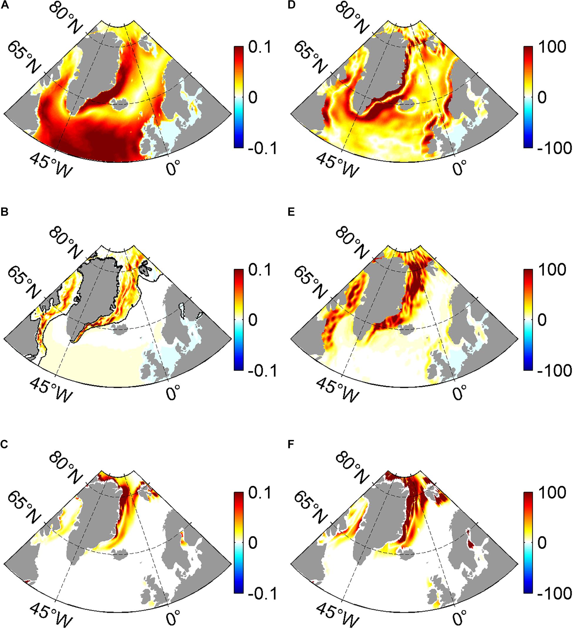
Figure 1. The time-mean ocean surface stress (N m^–2) in (A) CONTROL and the annual mean difference (B) between CONTROL and NONE (NONE minus CONTROL). (C) The annual mean difference in ocean surface stress with and without geostrophic currents in the ice-ocean stress calculation using the outputs from the CONTROL simulation (ocean surface stress without geostrophic currents minus that with geostrophic currents). Panels (D–F) is the same as in panels (A–C), but for Ekman pumping (m year^–1). The sea ice-covered regions are labeled in panel (B) by the black lines of 15% SIC in CONTROL averaged over the last decade.

TABLE 1

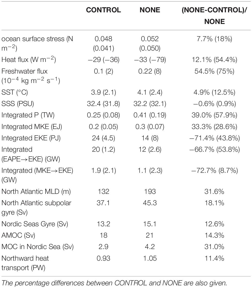
Table 1. Diagnostics in CONTROL and NONE averaged over the North Atlantic Ocean and the sea ice-covered region (values in the bracket).

As shown in Figure 1D, the spatial pattern of Ekman pumping is characterized by large values in the Nordic Seas, the Irminger Sea, and the Labrador Sea, especially in the region around the western boundary of the Greenland Sea (Figure 1D). Ekman pumping was calculated using $k\cdot \nabla \times (\frac{\mathrm{\tau }}{\mathrm{\rho }f})$, where k is the unit vector in the vertical direction, τ is the ocean surface stress, f is the Coriolis parameter, and ρ is the seawater density. The increase in the time-mean ocean surface stress also leads to a widespread enhancement in the magnitude of Ekman pumping in NONE, most noticeable in the Baffin Bay, the Labrador Sea, and the western boundary region of the Greenland Sea (Figure 1E). For example, the strength of the time-mean Ekman pumping averaged over the Nordic Seas is about 19% stronger in NONE than that in CONTROL; moreover, an increase of about 17% is also found in the Labrador Sea (Figure 1E).

Due to the scarcity of observations, the ocean surface currents were often replaced by surface geostrophic currents in previous studies when calculating ice-ocean stress (Yang, 2006, 2009; Zhong et al., 2018). Here, the different effects of including total ocean surface currents (ageostrophic and geostrophic components) or only including geostrophic currents on ice-ocean stress and Ekman pumping have also been examined (Figures 1C,F). Reducing the surface currents to their geostrophic component significantly impacts ice-ocean stress, especially in the Nordic Seas and the Labrador Sea (Figures 1B,C). The pattern and magnitude of ice-ocean stress calculated by the geostrophic component differ from that calculated by the total ocean surface currents, especially in the Labrador Sea, the Irminger Sea, and the Baffin Bay where the difference virtually disappears (Figures 1B,C). Similar results are also found in the Ekman pumping (Figures 1E,F). These above results indicate that the ageostrophic currents play an important role in the calculation of ice-ocean stress and Ekman pumping. When calculating the ice-ocean stress, the ageostrophic current should be properly considered in further studies rather than only the geostrophic current as done in previous studies (Yang, 2006, 2009; Zhong et al., 2018).

Figure 2 shows the time-mean net surface freshwater flux (the sum of evaporation, precipitation, runoff, and sea ice freezing/melting), net heat flux (the sum of sensible heat flux, latent heat flux, long-wave radiation, and short-wave radiation), SST, and sea surface salinity (SSS) averaged over the last decade in CONTROL and their differences between CONTROL and NONE. The overall patterns of time-mean surface freshwater and heat fluxes are very similar in both experiments, with an extensive heat loss in the North Atlantic and a significant freshwater input in the western boundary regions of the Greenland Sea and the Labrador Sea, seasonally covered by the sea ice (Figures 2A,D). In sea ice-covered regions, there is a significant enhancement in surface heat loss and freshwater input when ocean surface currents are excluded from ice-ocean stress calculation (Figures 2B,E). Heat loss (freshwater input) averaged over the sea ice-covered region in Figure 2B decreases by 54.4% (75%) from −79 W m^–2 (8 × 10^–4 kg m^–2 s^–1) in NONE to −36 W m^–2 (2 × 10^–4 kg m^–2 s^–1) in CONTROL (Table 1). However, the heat loss (freshwater input) in the North Atlantic Ocean in CONTROL decreased by 12.1% (54.5%) compared with that in NONE (Table 1). The differences in surface freshwater and heat fluxes between CONTROL and NONE are closely linked to their differences in SST and SSS (Figures 2C,F). The significant heat flux differences in the North Atlantic are in opposition to the SST differences, which demonstrates that changes in SST lead to changes in surface heat flux as well (Figures 2B,C). The following will show that the SST differences between CONTROL and NONE in the North Atlantic Ocean are mainly associated with differences in the strength of northward heat transport. As shown in Figure 2F, the SSS increases significantly over the sea ice-covered regions as a result of the stronger upwelling in NONE than that in CONTROL (Figures 1B,E), even with more freshwater entering into the ocean (Figure 2E). The freshwater flux induced by the sea ice melting\freezing is almost the same as the net freshwater flux (not shown). This confirms that more freshwater input in NONE comes from increased SST-induced sea ice melting than that in CONTROL. However, a slight decrease in SSS is also found in North Atlantic Ocean, which is caused by the spread of freshwater in NONE (Figures 2E,F and Table 1).

FIGURE 2

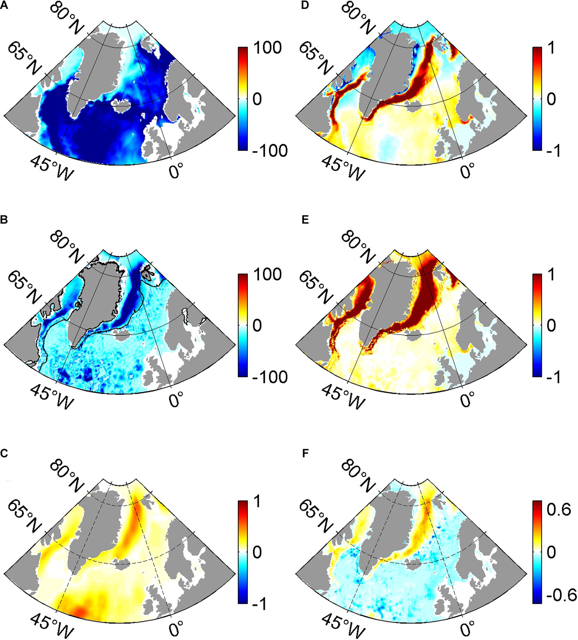
Figure 2. The time-mean net heat flux (W m^–2) in (A) CONTROL, and the annual mean differences of net heat flux (B) and SST (°C) (C) between CONTROL and NONE (NONE minus CONTROL). Panels (D–F) is the same as in panels (A–C), but for freshwater flux (10^–4 kg m^–2 s^–1) and SSS (PSU), respectively. The sea ice-covered regions are labeled in panel (B) by the black lines of 15% SIC in CONTROL averaged over the last decade. Negative values in panel (A) indicate the heat loss from the ocean. Moreover, negative values in panel (D) indicate that the ocean loses freshwater.

Mechanical Energy Input and Kinetic Energy

Figure 3A shows the time-mean distributions of the mechanical energy input to the time-mean currents by the time-mean ocean surface stress (P). It is calculated using $P=\overline{\mathrm{\tau }}\cdot \overline{u}$, where the over bar denotes a 10-year mean, τ is the ocean surface stress, and u is the ocean surface currents. The spatial patterns of P in both experiments are similar to those in previous studies (von Storch et al., 2012; Wu et al., 2017b), with most of the mechanical energy input concentrated in the central North Atlantic Ocean and the western boundary regions of the Greenland Sea, Labrador Sea, and Irminger Sea (Figure 3A). In NONE, the increase in P is significant, especially in the western boundary regions of the Irminger Sea, Labrador Sea, and Greenland Sea (Figure 3B). This increase is much more pronounced in wintertime (not shown). Figure 3C shows the distribution of mechanical energy input to time-varying ocean velocity by time-varying ocean surface stress ($P^{\prime }=\overline{{\mathrm{\tau }}^{\prime }\cdot u^{\prime }}$) in CONTROL, which is an energy source of eddy kinetic energy (EKE) and characterized by large values in the Denmark Strait, the North Atlantic Ocean, and the Labrador Sea. Similarly, the difference in P′ between CONTROL and NONE is most significant in the western boundary regions of the Irminger Sea, the Labrador Sea, and the Greenland Sea, where there are the seasonally sea ice-covered regions (Figure 3D).

FIGURE 3

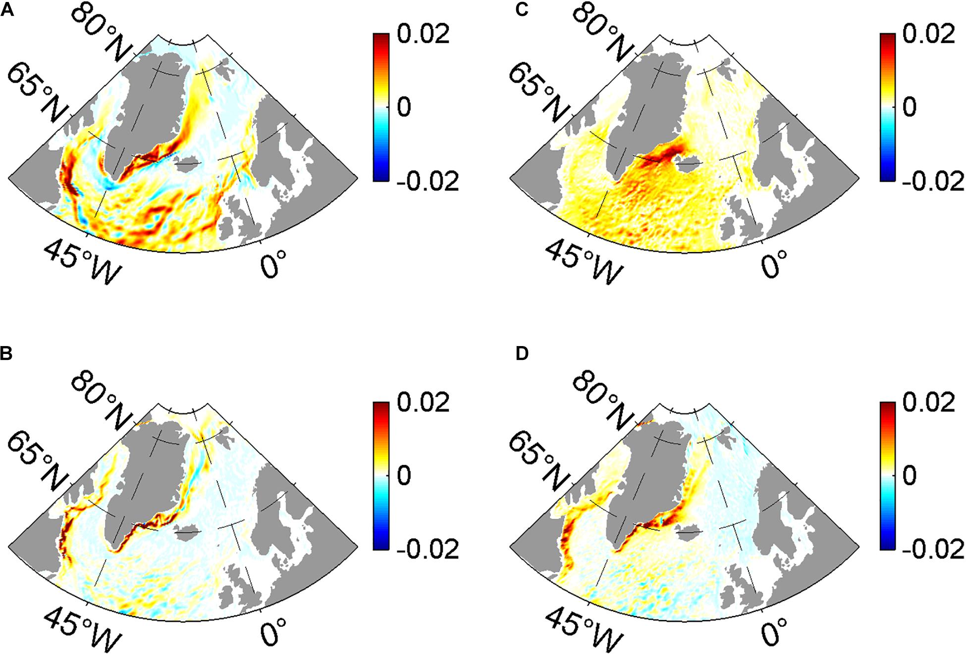
Figure 3. The time-mean mechanical energy input to the ocean by the time-mean ocean surface stress (W m^–2) in (A) CONTROL, and the (B) difference between CONTROL and NONE (NONE minus CONTROL). Panels (C,D) is the same as in panels (A,B), but for time-varying mechanical energy input to the ocean by the time-varying ocean surface stress (W m^–2) and their difference.

The spatial integrated value of P(P′) decreases by 39.0% (41.7%) from 0.41 TW (1 TW = 10¹² W; 0.24 TW) in NONE to 0.25 TW (0.14 TW) in CONTROL. Considering the ocean surface currents in the ice-ocean stress calculation results in a decrease in P (P′) by 0.16 TW (0.1 TW), of which 0.1 TW (0.07 TW) is due to a decrease in $\overline{\mathrm{\tau }}\cdot {\overline{u}}_{ag}$ ($\overline{{\mathrm{\tau }}^{\prime }\cdot u_{ag}^{\prime }}$), and only 0.06 TW (0.03 TW) is due to a decrease in $\overline{\mathrm{\tau }}\cdot {\overline{u}}_g$ ($\overline{{\mathrm{\tau }}^{\prime }\cdot u_g^{\prime }}$), where the prime denotes the derivation from the 10-year mean; u_ag and u_g are the ageostrophic and geostrophic components of the ocean surface currents, respectively.

The effects of considering ocean surface currents in the ice-ocean stress calculation on the EKE and mean kinetic energy (MKE) are also investigated. The EKE and MKE are defined as $\text{EKE}=0.5\cdot \overline{(u^{\prime }+v^{\prime })}$ and $\text{MKE}=0.5\cdot ({\overline{u}}^2+{\overline{v}}^2)$’ where u and v are the zonal and meridional ocean currents, respectively. Similar to the previous studies (Eden and Böning, 2002; Rieck et al., 2019), the distributions of the time-mean MKE and EKE are characterized by large values along the boundary currents over the Irminger Sea, the Labrador Sea, the Greenland Sea, and in the vicinity of the North Atlantic Current branches (Figures 4A,C). When ocean surface currents are excluded from the ice-ocean stress calculation, there is a resultant increase in the surface MKE over the North Atlantic Ocean, most notably in the western boundary regions of the Labrador Sea, the Irminger Sea, and the Greenland Sea (Figure 4B). There is an EKE increase in the western boundary region of the Greenland Sea and the Baffin Bay where there are seasonally sea ice-covered regions (Figure 4D). It will be shown later that this EKE increase is due to the combined effect of the energy conversion from eddy available potential energy (EAPE) and MKE to EKE, which is induced by a stronger mechanical energy input (Figures 1B,E, 3B,D). However, the significant reduction of EKE is found in NONE across the North Atlantic Ocean and Nordic Seas (Figure 4D), which is due to the stable water column induced by more freshwater input in NONE than that in CONTROL, as previously shown (Zhong et al., 2018). Quantitatively, integrated MKE over the entire region decreases by about 33.3% from 0.3 EJ (1 EJ = 10¹⁸ J) in NONE to 0.2 EJ in CONTROL (Table 1). Spatially integrated over sea ice-covered regions, EKE in CONTROL and NONE are 4.5 PJ (1 PJ = 10¹⁵ J) and 8 PJ, respectively, representing a 43.8% reduction from CONTROL (NONE minus CONTROL) (Figure 4D). Although the magnitude of the MKE and EKE reduction weakens with depth, the reduction percentage of the area-averaged MKE and EKE remains roughly 10 and 25% deeper than 300 m (not shown).

FIGURE 4

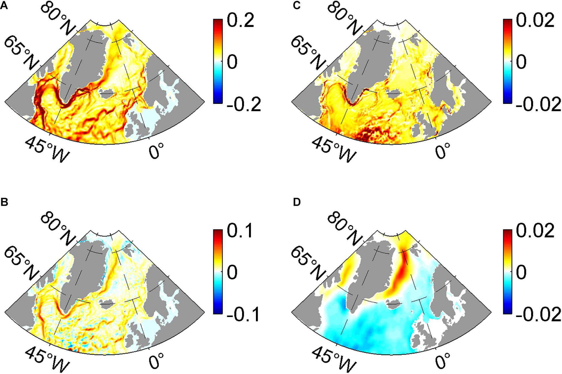
Figure 4. The distributions of (A) time-mean ocean surface MKE (m² s^–2) and the (B) difference between CONTROL and NONE (NONE minus CONTROL). Panels (C,D) is the same as in panels (A,B), but for the time-mean ocean surface EKE (m² s^–2) and their difference.

The energy budget of EKE and MKE has also been calculated to explain the change in kinetic energy when considering the ocean surface currents in the ice-ocean stress calculation. The formulas used to calculate the energy conversion between EKE and MKE are the same as those used in Wu et al. (2017a). Figure 5A presents the distribution of vertically integrated energy conversion from EAPE to EKE through the baroclinic pathway. The energy is converted from EAPE to EKE (positive value) in the North Atlantic Ocean, the Labrador Sea, and the Nordic Seas (Figure 5A), which is similar to the previous studies (Eden and Böning, 2002; von Storch et al., 2012; Rieck et al., 2019). In NONE, a strengthened Ekman pumping leads to a more titled isopycnal that contains more available potential energy (APE) in the western boundary regions of the Nordic Seas and the Baffin Bay, which is released through the baroclinic pathway (Figure 5B). However, there is a reduction in the energy conversion from EAPE to EKE in the broad North Atlantic Ocean and the Labrador Sea (Figure 5B). Enhanced sea ice melting results in more freshwater input to the Labrador Sea and the North Atlantic Ocean in NONE than in CONTROL (Figures 2E,F), so stratification is much more stable there. Spatially integrated, the energy conversion from EAPE to EKE is 20 GW (1 GW = 10⁹ TW) in CONTROL, while it decreases to 12 GW in NONE, representing a 66.7% reduction.

FIGURE 5

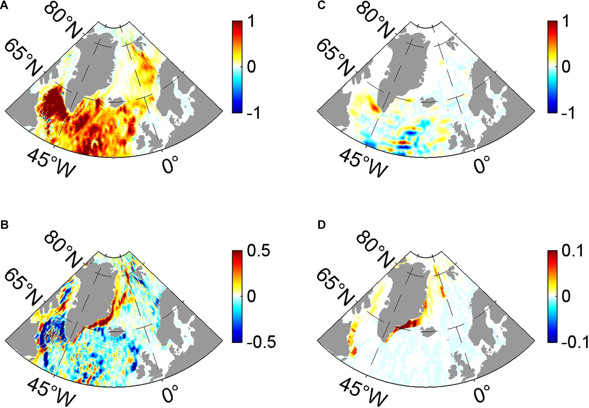
Figure 5. The distributions of (A) vertically integrated energy conversion rate from EAPE to EKE (10^–1 W m^–2) and the (B) difference between CONTROL and NONE (NONE minus CONTROL). Panels (C,D) is the same as in panels (A,B), but for the energy conversion rate from MKE to EKE (10^–1 W m^–2) and their difference.

In addition, the EKE can also obtain energy directly from the MKE through the barotropic pathway. Figure 5C gives the vertically integrated distribution of energy conversion from MKE to EKE, with a large energy conversion rate from MKE to EKE (positive values) in the Labrador Sea, especially in the west Greenland current region, which is similar to the previous studies (Eden and Böning, 2002; von Storch et al., 2012; Wu et al., 2016, 2017b; Rieck et al., 2019). When ocean surface currents are excluded from the ice-ocean stress calculation, the shear instability between sea ice drift and ocean surface velocity is strengthened in the sea ice-covered regions, such as in the western boundary regions of the Nordic Seas, the Irminger Sea, and the Labrador Sea (Figure 5D). Integrated over the North Atlantic Ocean (sea ice-covered region), the energy conversion from MKE to EKE is 1.9 GW (2.1 GW) in CONTROL, while it decreases to 1.1 GW (2.3 GW) in NONE, accounting for a 72.7% (−8.7%) decrease.

Sea Ice

The changed air-sea fluxes and SST induced by the increased ice-ocean stress in NONE can be fed back to the overlying sea ice. As shown in Figure 6A, the SIC decreases extensively in NONE, especially in the western boundary regions of the Baffin Bay, the Labrador Sea, the Irminger Sea, and the Greenland Sea (Figure 6A). Quantitatively, the annual mean SICs in CONTROL and NONE are 33 and 22%, respectively, representing a 33.3% decrease with respect to CONTROL; the winter mean values are 47 and 22%, respectively, representing a 53.2% decrease with respect to CONTROL. In NONE, the sea ice extent (SIE) also expands dramatically, as shown by the labeled lines of 15% SIC in Figure 6, especially in the Nordic Seas (Figures 6A,B). Similarly, the sea ice thickness (SIT) also decreases significantly as large as 0.2 m in the western boundary regions of the Nordic Seas (Figure 6C); this decrease is much larger in the wintertime, amounting to 0.5 m (Figure 6D). Besides, there is a time-mean reduction of 27.6% (0.76 m in CONTROL and 0.55 m in NONE) and 29.6% (0.81 m in CONTROL and 0.57 m in NONE) of SIT from CONTROL to NONE throughout the whole year and wintertime, respectively (Figures 6C,D).

FIGURE 6

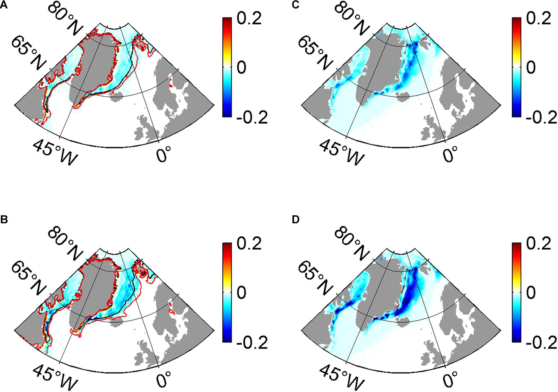
Figure 6. The distributions of annual mean SIC difference (A) and the wintertime-mean SIC difference (B) between CONTROL and NONE (NONE minus CONTROL). Panels (C,D) is the same as in panels (A,B) but for the SIT (m) and their difference. The labeled lines are 15% SIC in CONTROL (black) and NONE (red) averaged over the last decade, respectively.

Figures 7A,B show the monthly mean total sea ice volume (SIV) and SIE in both simulations over the Arctic Ocean (regions where the SIC is equal to or greater than 15%). The SIE is much larger in NONE than in CONTROL. Quantitatively, the time-mean SIE in September decreases from 5.5 × 10⁶ km² in NONE to 4.5 × 10⁶ km² in CONTROL over the Arctic Ocean. As analyzed above, the significant increase in SIE is attributed to increased sea ice transport caused by greater ice-ocean stress in NONE. However, the total monthly SIV over the Arctic Ocean decreases entirely in NONE (Figure 7B). For example, the SIV in September decreases from 1.9 × 10⁴ km³ in CONTROL to 1.8 × 10⁴ km³ in NONE. The reduction in SIV is caused by a much thinner SIT in NONE than in CONTROL (Figures 6C,D). As shown above, the changes in SIE and SIV are the combined effect of increased ice-ocean stress and higher SST.

FIGURE 7

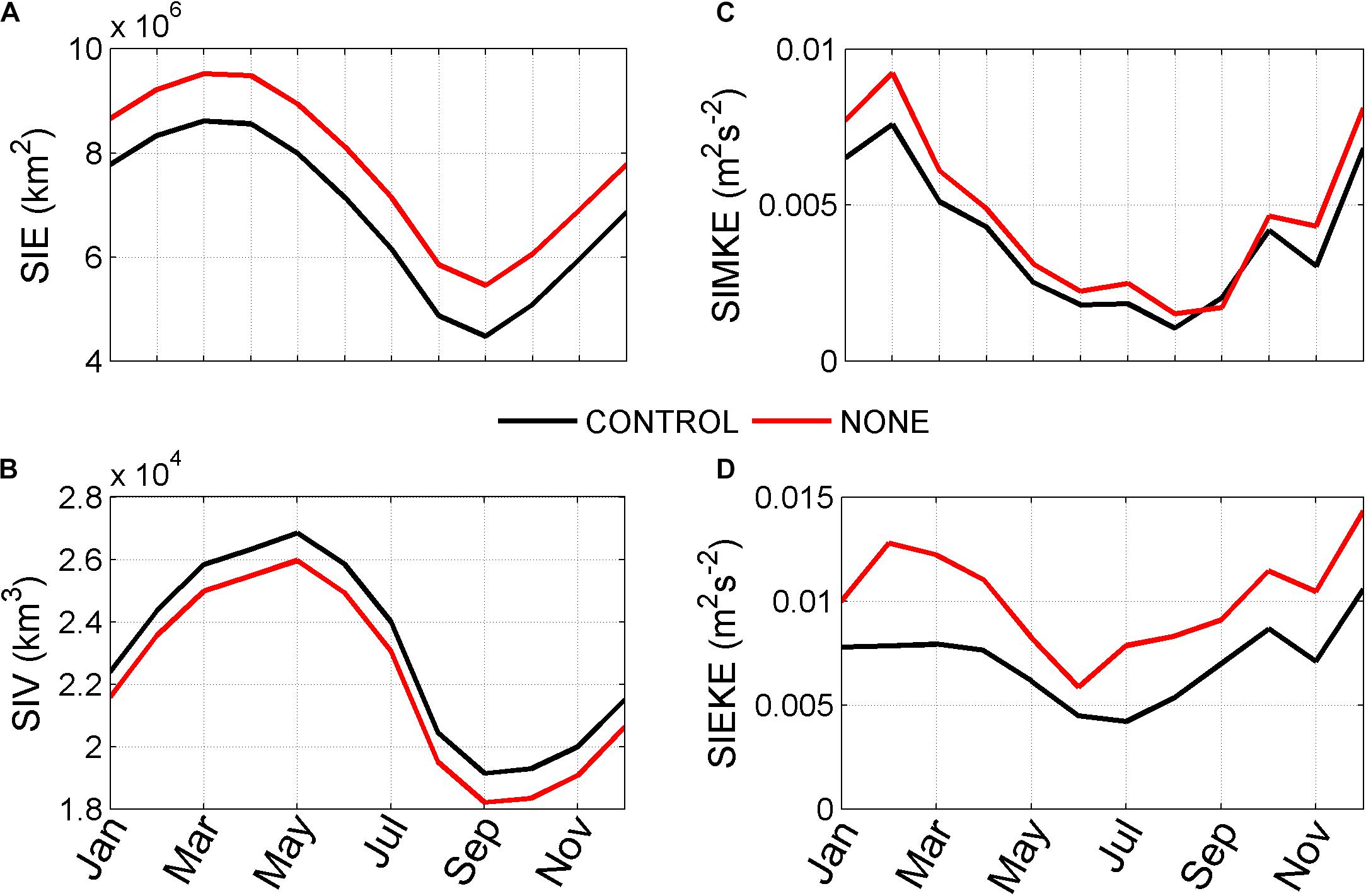
Figure 7. The monthly simulated Arctic (A) SIE (km²), (B) SIV (km³), (C) SIMKE (m^–2 s^–2), and (D) SIEKE (m^–2 s^–2) of Arctic sea ice in CONTROL (black) and NONE (red).

The mean kinetic energy (SIMKE) and eddy kinetic energy (SIEKE) of sea ice over the Arctic Ocean are also presented in both simulations (Figures 7C,D). The SIMKE and SIEKE are defined as $\text{SIMKE}=0.5\cdot ({\overline{u}}_i^2+{\overline{v}}_i^2)$ and ${\text{SIEKE}}_i=0.5\cdot \overline{(u_i^{\prime }+v_i^{\prime })}$, where u_i and v_i are the zonal and meridional sea ice velocity, respectively. In NONE, the movement of the sea ice becomes more active than that in CONTROL, and both SIMKE and SIEKE increase visibly. For example, the time-mean and area-mean SIMKE decreases from 0.0047 m^–2 s^–2 in NONE to 0.0039 m^–2 s^–2 in CONTROL (Figure 7C); besides, SIEKE also decreases greatly from 0.01 m^–2 s^–2 in NONE to 0.007 m^–2 s^–2 in CONTROL (Figure 7D).

Subpolar Gyres, Mixed Layer Depth, and Meridional Overturning Circulation

Differences in the depth-integrated meridional volume transport and the gyre circulations between NONE and CONTROL are likely to be induced by the differences in the time-mean Ekman pumping. Figure 8A presents the time-mean barotropic stream function in CONTROL, which is similar to previous studies, characterized by cyclonic gyres in the North Atlantic Ocean and the Nordic Seas (Wu et al., 2016, 2017b). Figure 8B shows that the strength of the simulated subpolar gyre reduces almost everywhere when considering ocean surface currents in the ice-ocean stress calculation. For example, the strength of the time-mean subpolar gyre in the North Atlantic Ocean decreases by about 18.1% from 45.3 Sv in NONE to 37.1 Sv in CONTROL, and that of the gyre in the Nordic Seas reduces by about 12.6% from 15.1 Sv in NONE to 13.2 Sv in CONTROL.

FIGURE 8

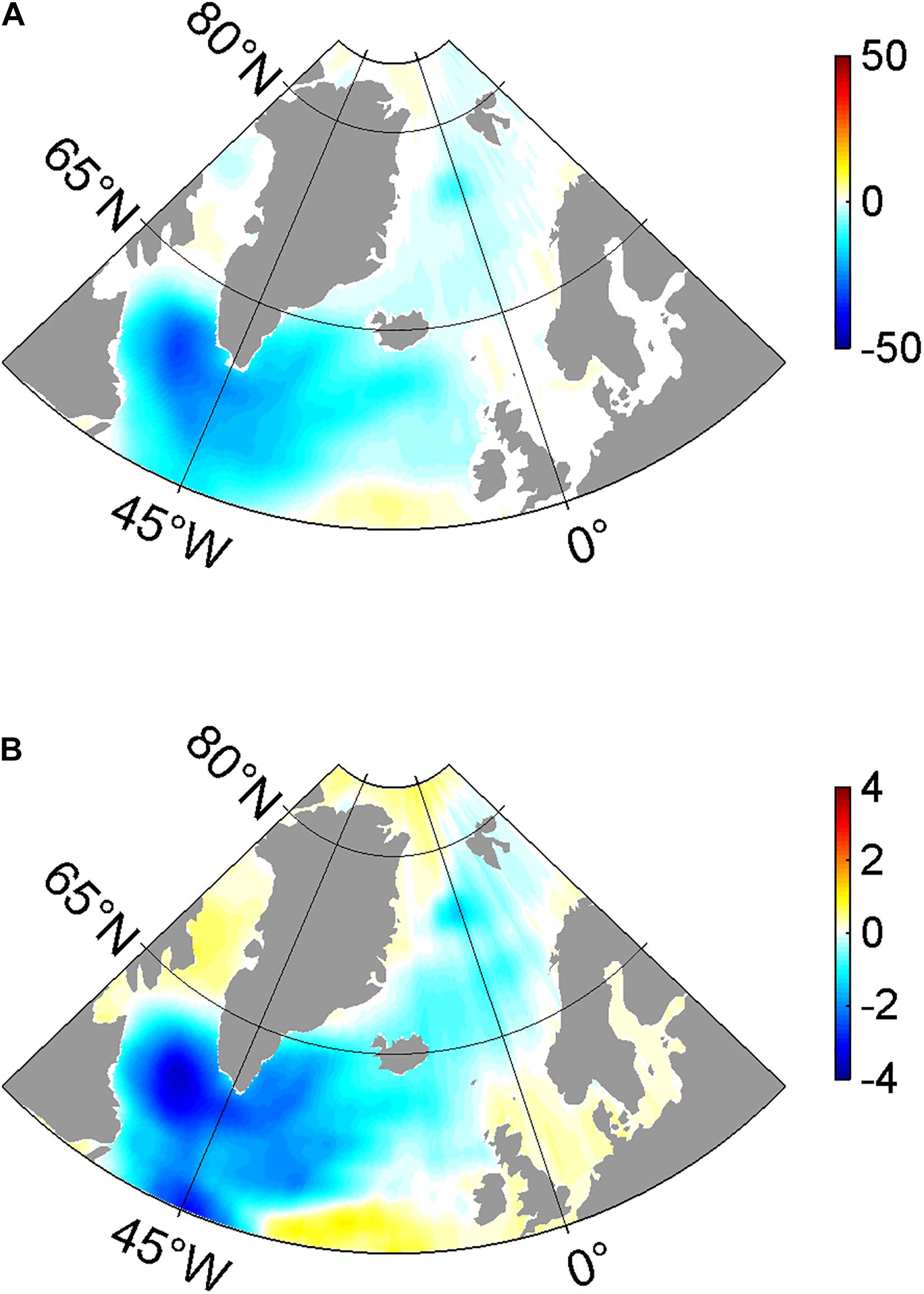
Figure 8. The distributions of (A) time-mean barotropic stream function (Sv) in CONTROL and their difference (B) between CONTROL and NONE (NONE minus CONTROL).

We now investigate the impacts of considering ocean surface currents in ice-ocean stress calculation on MLD in the Nordic Seas and North Atlantic Ocean. The MLD is defined similarly to previous studies (Downes et al., 2009; Liu et al., 2017; Wu et al., 2020) as the depth at which the potential density is 0.03 kg m^–3 larger than that at the surface. The time-mean patterns of the MLD and the differences between NONE and CONTROL are shown in Figures 9A–C. The simulated MLDs in both experiments are represented by deep MLD in the Labrador Sea and Nordic Seas (Figure 9A), which is similar to the results from previous investigations (Kara and Rochford, 2003; Holdsworth and Myers, 2015; Wu et al., 2016). It is noted that the MLD is deeper than the observations, which is induced by a higher surface salinity than that from the observations. Additionally, the model resolution is relatively coarse, especially at the subpolar latitudes, and thus likely underestimates the role played by eddies in the restratification process after deep convection events. Excluding ocean surface currents from the ice-ocean stress calculation, the MLD increases considerably in the Labrador Sea and the Nordic Seas (Figure 9B). This increase is also more significant in wintertime (Figure 9C). For example, the time-mean MLDs averaged in the Labrador Sea (Nordic Seas) are 2,750 and 3,450 m (210 and 407 m) in CONTROL and NONE, respectively, representing a 20.3% (48.4%) increase. This difference amounts to 34 and 61% averaged over the Labrador Sea and the Nordic Seas in wintertime (Figure 9C). As shown in Figure 1E, in CONTROL, considering ocean surface currents in the ice-ocean stress calculation reduces the ocean surface stress and wind stress curl in the subpolar North Atlantic. For example, Ekman pumping is about 12.1% weaker in CONTROL than that in NONE with respect to the average for the Labrador Sea. The reduced wind stress curl weakens the strength of Ekman pumping and results in less doming of the density surface and a weaker cyclonic circulation over the Labrador Sea in CONTROL than that in NONE (Figure 8B). This reduced effect of pre-conditioning then makes it harder for sea surface heat loss to overcome stratification and trigger deep-reaching convection in CONTROL (Marshall and Schott, 1999).

FIGURE 9

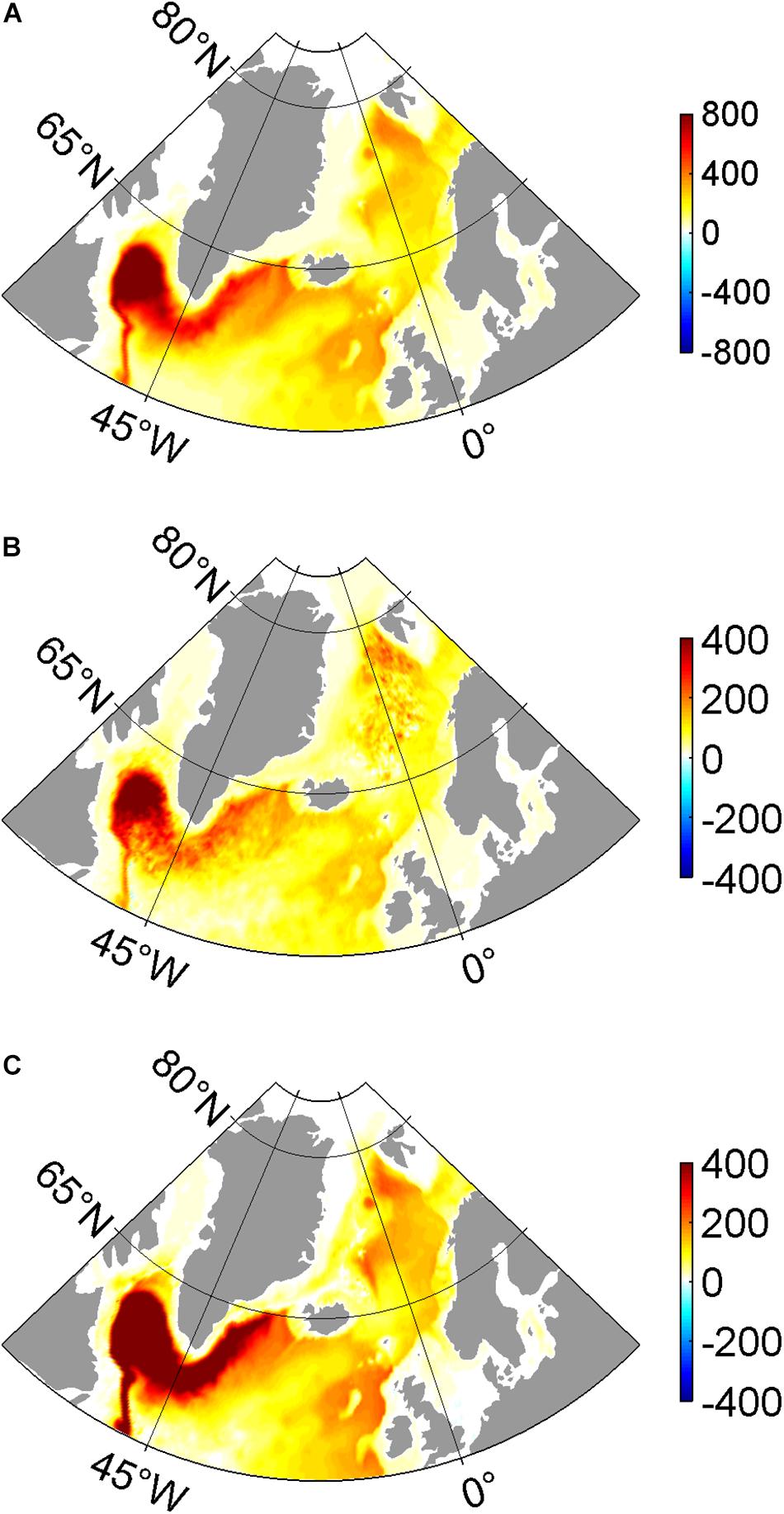
Figure 9. The distributions of (A) winter (January, February, and March) time-mean MLD (m) in CONTROL and their differences (B) between CONTROL and NONE averaged over the last decade, and their difference (C) averaged over the winter season (NONE minus CONTROL).

The changes in the intensity of deep convection between these two experiments in the Labrador Sea and the Nordic Seas correlate with the differences in the strength of AMOC and MOC in the Nordic Seas, as found in previous studies (Eden and Willebrand, 2001; Zhai et al., 2011; Zhai and Johnson, 2014; Wu et al., 2016). The definition of MOC is similar to that in Wu et al. (2016, 2020) by integrating the meridional velocity across the ocean basin from the western boundary (x_W) to eastern boundary (x_E), and from the ocean bottom at z = −h upward: $\mathrm{\psi }(y,z,t)={\int }_{-h}^z{\int }_{x_W(y,z)}^{x_E(y,z)}v(x,y,z,t)\mathit{d}x\mathit{d}z$. The maximum value of ψ is defined as the strength of the MOC. The structure of AMOC is familiar in both simulations, with light water transports northward and dense water transports southward (Figure 10A; Wunsch and Heimbach, 2013; Wu et al., 2016). As shown in Figure 10B, when ocean surface currents are excluded, the strength of the simulated AMOC is coherently enhanced at all latitudes by as much as 3 Sv, representing a 14.3% reduction (Table 1). Besides, Figure 11A shows the distribution of the MOC in the Nordic Seas, which shows a similar structure in both simulations, with the light water transports northward and the dense water transports southward. In NONE, the strength of the simulated MOC in Nordic Seas is coherently enhanced at all latitudes (Figure 11B). The maximum MOC strength in Nordic Seas decreases by about 31.0% from 4.2 Sv in NONE to 2.9 Sv in CONTROL. One of the roles of the ocean in the climate system is the transport of heat to high latitudes. The meridional heat transport (MHT) can be adequately approximated (Warren, 1999; Zhang et al., 2002; Msadek et al., 2013) by $\mathrm{\rho }{C}_p{\int }_0^L{\int }_{-H}^{0}vT\mathit{d}z\mathit{d}x$, where C_p is the specific heat capacity of seawater, T is the potential temperature, H and L are the depth and width of the ocean, respectively. In the Atlantic Ocean, the structures of MHT in both simulations are similar to the observed and simulated results (not shown, Ganachaud and Wunsch, 2003; Wu et al., 2016). For example, the maximum MHT is found to be 0.93 PW (1 PW = 10¹⁵ W) in CONTROL at 25°N, which is comparable to the 1.07 ± 0.26 PW and 1.27 ± 0.15 PW estimated in the previous studies (Macdonald, 1998; Ganachaud and Wunsch, 2003). In comparison, the maximum MHT increases to 1.05 PW in NONE, representing a 13% enhancement. It is noted that the MHT in NONE is closer to observations than that in CONTROL. It is likely caused by the weaker AMOC in ECCO2 than that in observations (Ganachaud and Wunsch, 2003), as the strength of AMOC dominates the MHT in the Atlantic Ocean.

FIGURE 10

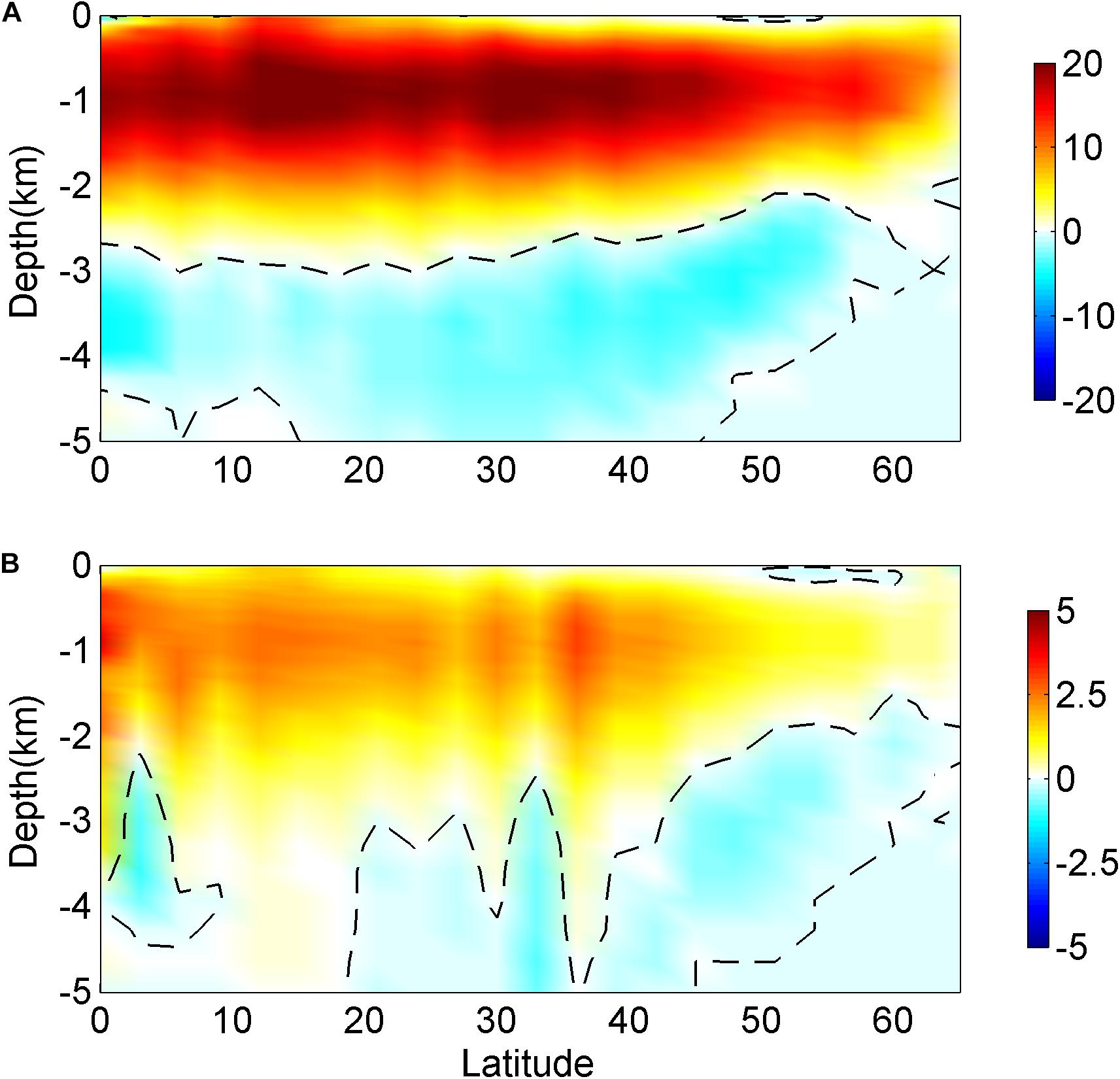
Figure 10. The distributions of (A) time-mean AMOC (Sv) in CONTROL and their differences (B) between CONTROL and NONE (NONE minus CONTROL).

FIGURE 11

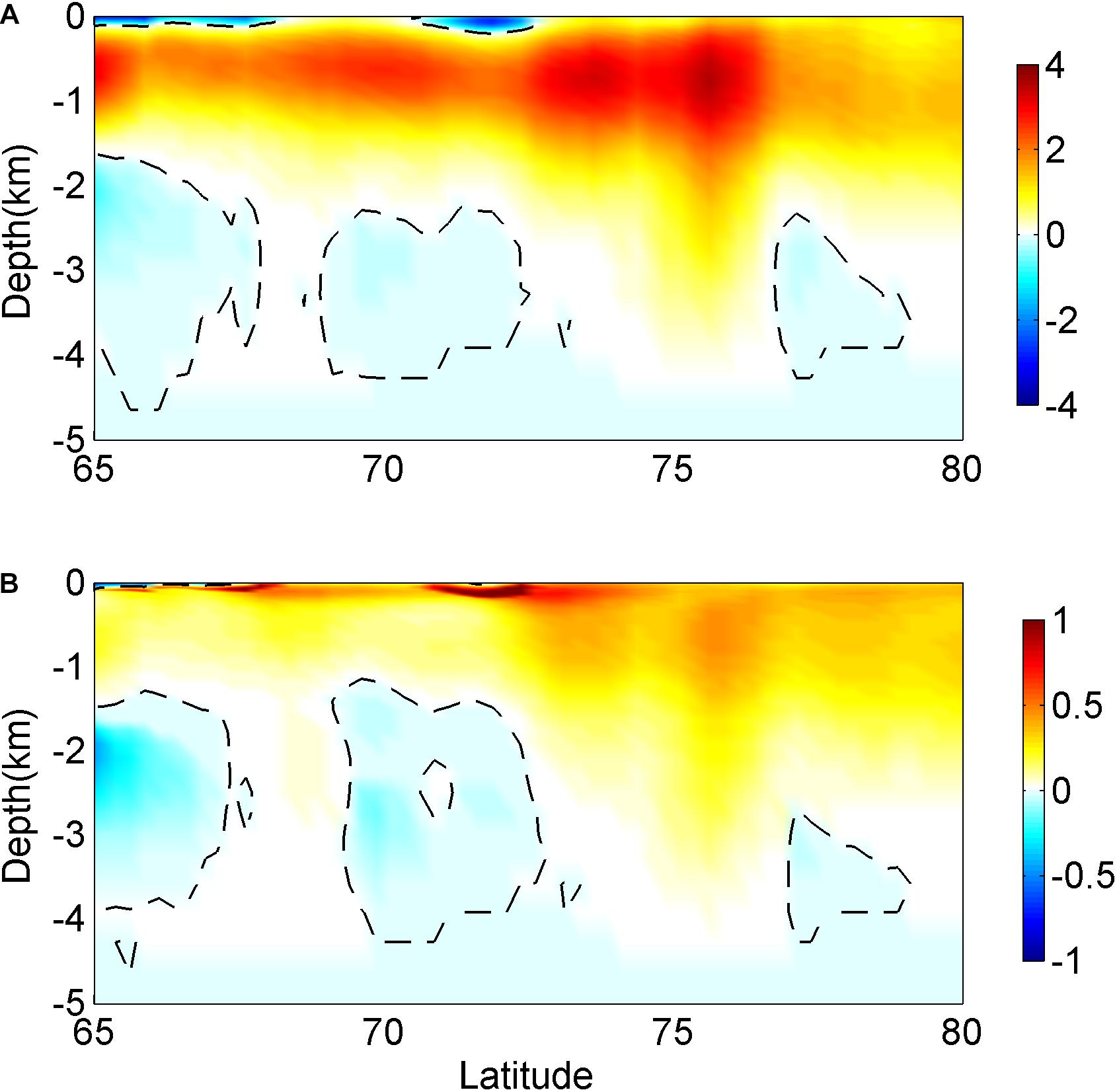
Figure 11. The distributions of (A) time-mean MOC (Sv) in the Nordic Seas in CONTROL and their differences (B) between CONTROL and NONE (NONE minus CONTROL).

Conclusion and Discussion

In this study, we have investigated for the first time the impact of considering ocean surface currents in the ice-ocean stress calculation on the North Atlantic Ocean and Arctic sea ice using a global coupled ocean-sea ice model with approximately 18-km resolution. By comparing these simulations with inclusion and exclusion of the ocean surface currents in ice-ocean stress calculation, we find that:

• Including ocean surface currents in the ice-ocean stress calculation leads to a broad reduction in the magnitude of the ocean surface stress and Ekman pumping over the North Atlantic Ocean by about 7.7 and 15%, respectively. Ageostrophic currents play an important role in the ice-ocean stress and Ekman pumping calculations, indicating that ageostrophic currents should be properly considered in subsequent studies when calculating the ice-ocean stress. In addition, a significant decrease in freshwater input is also found in the sea ice-covered Labrador Sea and Nordic Seas resulting from less sea ice melting.

• Considering ocean surface currents in the ice-ocean stress calculation reduces mechanical energy input to total surface currents by about 0.26 TW (about 40% decrease), and the mechanical energy input to surface ageostrophic and geostrophic motions decreases by about 0.17 and 0.09 TW, respectively.

• Including ocean surface currents in the ice-ocean stress considerably damps both EKE and MKE in the sea ice-covered ocean, by about 43.8 and 28.6%, respectively. The reduction in EKE is mainly induced by the baroclinic pathway, especially in the Labrador Sea and the North Atlantic. The reduction in MKE is mainly induced by the barotropic pathway, especially in the boundary regions of the Labrador Sea and the Nordic Seas.

• Including ocean surface currents in the ice-ocean stress leads to an 18.1% decrease in the strength of the subpolar gyre in the North Atlantic Ocean. It also weakens the intensity of deep convection in the northern North Atlantic Ocean and the Nordic Seas by about 20.3 and 48.4%. Additionally, the strengths of AMOC and MOC in the Nordic Seas decrease by about 14.3 and 31%, respectively.

• The weakening of the AMOC leads to a reduction in the maximum northward ocean heat transport in the Atlantic Ocean by 0.12 PW. This reduction results in lower SST and reduced surface heat loss in the northern North Atlantic Ocean and the Nordic Seas. The decrease in mechanical energy input and SST leads to a shrink in the SIE and an attenuation of the SIT.

It is worth noting that this study has several limitations. For example, the model used here is only at the eddy-permitting resolution in the low and middle latitudes. It is too coarse in the North Atlantic and the Nordic Seas (Nurser and Bacon, 2014). Therefore, the reduction in EKE induced by the relative ice-ocean stress is likely to be underestimated, since the damping effect is proportional to the magnitude of the surface kinetic energy. Although the differences in the model results averaged over different time periods are inconspicuous, our results may depend quantitatively on the model. Therefore, results from multiple models need to be compared for further study. The atmospheric forcing used here is relatively coarse (six-hourly mean, 1.125° × 1.125°). Many mesoscale and synoptic atmospheric phenomena, which are important in the sea ice drift and the ocean general circulation, are missed (Wu et al., 2016, 2020). In addition, the impact of including ocean surface currents in the ice-ocean stress calculation is very important for the Southern Ocean simulations. For example, Kim et al. (2017) found that the seasonal variability of the circumpolar deep water warm layer thickness can be explained by the variability of Ekman pumping induced by horizontally varying wind and sea ice drift when considering the ocean surface currents in τ_IO calculation on the Amundsen Sea continental shelf. Therefore, further research is needed to consider the potential impact of ocean surface currents in the ice-ocean stress calculation for the Southern Ocean and even the global ocean climate system.

Data Availability Statement

The original contributions presented in the study are included in the article/supplementary material, further inquiries can be directed to the corresponding author/s.

Author Contributions

YW performed the methodology, ran the numerical model, data analyses, and wrote the original manuscript draft. YW, ZW, and CL participated in the manuscript revision and improvement. All authors contributed to the article and approved the submitted version.

Funding

This study was supported by the National Natural Science Foundation of China (Grant Nos. 41806216, 41941007, and 41876220), by the China Postdoctoral Science Foundation (Grant Nos. 2019T120379 and 2018M630499), and by the Talent start-up fund of Nanjing Xiaozhuang University (Grant No. 4172111).

Conflict of Interest

The authors declare that the research was conducted in the absence of any commercial or financial relationships that could be construed as a potential conflict of interest.

Acknowledgments

The MITgcm code was obtained freely from http://mitgcm.org/. The atmospheric forcing data were obtained freely from the NCAR’s research data archive (JRA-55: https://rda.ucar.edu/datasets/ds625.0/). We thank the editor and two reviewers for their positive and constructive comments and suggestions.

References

Abernathey, R. P., Cerovecki, I., Holland, P. R., Newsom, E., Mazloff, M., and Talley, L. D. (2016). Water-mass transformation by sea ice in the upper branch of the southern ocean overturning. Nat. Geosci. 9, 596–601. doi: 10.1038/ngeo2749

CrossRef Full Text | Google Scholar

Adcroft, A., Campin, J. M., Hill, C., and Marshall, J. (2004). Implementation of an atmosphere- ocean general circulation model on the expanded spherical cube. Mon. Wea. Rev. 132, 2845–2863. doi: 10.1175/mwr2823.1

CrossRef Full Text | Google Scholar

Brakstad, A., Våge, K., Håvik, L., and Moore, G. W. K. (2019). Water mass transformation in the Greenland Sea during the period 1986-2016. J. Phys. Oceanogr. 49, 121–140. doi: 10.1175/jpo-d-17-0273.1

CrossRef Full Text | Google Scholar

Campbell, E. C., Wilson, E. A., Moore, G. W. K., Riser, S. C., Brayton, C. E., Mazloff, M. R., et al. (2019). Antarctic offshore polynyas linked to southern hemisphere climate anomalies. Nature 570, 1–7.

Google Scholar

Chu, P. C. (1986). An instability theory of ice-air interaction for the migration of the marginal ice zone. Geophys. J. Int. 86, 863–883. doi: 10.1111/j.1365-246x.1986.tb00665.x

CrossRef Full Text | Google Scholar

Dawe, J. T., and Thompson, L. (2006). Effect of ocean surface currents on wind stress, heat flux, and wind power input to the ocean. Geophys. Res. Lett. 33:L09604. doi: 10.1029/2006GL025784

CrossRef Full Text | Google Scholar

Deng, Z., Xie, L., Liu, B., Wu, K., Zhao, D., and Yu, T. (2009). Coupling winds to ocean surface currents over the global ocean. Ocean Modell. 29, 261–268. doi: 10.1016/j.ocemod.2009.05.003

CrossRef Full Text | Google Scholar

Dewey, S., Morison, J., Kwok, R., Dickinson, S., Morison, D., and Andersen, R. (2018). Arctic ice-ocean coupling and gyre equilibration observed with remote sensing. G Geophys. Res. Lett. 45, 1499–1508. doi: 10.1002/2017gl076229

CrossRef Full Text | Google Scholar

Doddridge, E. W., and Marshall, J. (2017). Modulation of the seasonal cycle of Antarctic sea ice extent related to the Southern Annular Mode. Geophys. Res. Lett. 44, 9761–9768. doi: 10.1002/2017gl074319

CrossRef Full Text | Google Scholar

Dotto, T. S., Naveira Garabato, A., Bacon, S., Tsamados, M., Holland, P., Hooley, J., et al. (2018). Variability of the ross gyre, southern ocean: drivers and responses revealed by satellite altimetry. Geophys. Res. Lett. 45, 6195–6204.

Google Scholar

Downes, S. M., Bindoff, N. L., and Rintoul, S. R. (2009). Impacts of climate change on the subduction of mode and intermediate water masses in the Southern Ocean. J. Climat. 22, 3289–3302. doi: 10.1175/2008jcli2653.1

CrossRef Full Text | Google Scholar

Duhaut, T. H. A., and Straub, D. N. (2006). Wind stress dependence on ocean surface velocity: implications for mechanical energy input to ocean circulation. J. Phys. Oceanogr. 36, 202–211. doi: 10.1175/jpo2842.1

CrossRef Full Text | Google Scholar

Eden, C., and Böning, C. (2002). Sources of eddy kinetic energy in the Labrador Sea. J. Phys. Oceanogr. 32, 3346–3363. doi: 10.1175/1520-0485(2002)032<3346:soekei>2.0.co;2

CrossRef Full Text | Google Scholar

Eden, C., and Dietze, H. (2009). Effects of mesoscale eddy/wind interactions on biological new production and eddy kinetic energy. J. Geophys. Res. 114:C05023.

Google Scholar

Eden, C., and Willebrand, J. (2001). Mechanism of interannual to decadal variability of the North Atlantic circulation. J. Climate. 14, 2266–2280. doi: 10.1175/1520-0442(2001)014<2266:moitdv>2.0.co;2

CrossRef Full Text | Google Scholar

Ganachaud, A., and Wunsch, C. (2003). Large-scale ocean heat and freshwater transports during the World Ocean Circulation Experiment. J. Climate 16, 696–705. doi: 10.1175/1520-0442(2003)016<0696:lsohaf>2.0.co;2

CrossRef Full Text | Google Scholar

Goosse, H., and Fichefet, T. (1999). Importance of ice-ocean interactions for the global ocean circulation: a model study. J. Geophys. Res. 104, 23337–23355. doi: 10.1029/1999jc900215

CrossRef Full Text | Google Scholar

Gordon, A. L. (1978). Deep antarctic convection west of maud rise. J. Phys. Oceanogr. 8, 357–377.

Google Scholar

Haumann, F. A., Gruber, N., Münnich, M., Frenger, I., and Kern, S. (2016). Sea-ice transport driving Southern Ocean salinity and its recent trends. Nature 537, 89–92. doi: 10.1038/nature19101

PubMed Abstract | CrossRef Full Text | Google Scholar

Hibler, W. D. (1979). A dynamic thermodynamic sea ice model. J. Phys.Oceanogr. 9, 815–846. doi: 10.1175/1520-0485(1979)009<0815:adtsim>2.0.co;2

CrossRef Full Text | Google Scholar

Hibler, W. D., and Ackley, S. F. (1983). Numerical simulation of the weddell sea pack ice. J. Geophys. Res. 88, 2873–2887.

Google Scholar

Holdsworth, A. M., and Myers, P. G. (2015). The influence of highfrequency atmospheric forcing on the circulation and deep convection of the Labrador Sea. J. Climate 28, 4980–4996. doi: 10.1175/jcli-d-14-00564.1

CrossRef Full Text | Google Scholar

Holland, P. R., and Kwok, R. (2012). Wind-driven trends in Antarctic sea-ice drift. Nat. Geosci. 5, 872–875. doi: 10.1038/ngeo1627

CrossRef Full Text | Google Scholar

Hosking, J. S., Orr, A., Marshall, G. J., Turner, J., and Phillips, T. (2013). The influence of the Amundsen-Bellingshausen Seas low on the climate of West Antarctica and its representation in coupled climate model simulations. J. Climate 26, 6633–6648. doi: 10.1175/jcli-d-12-00813.1

CrossRef Full Text | Google Scholar

Hughes, C. W., and Wilson, C. (2008). Wind work on the geostrophic ocean circulation: an observational study on the effect of small scales in the wind stress. J. Geophys. Res. 113:4371.

Google Scholar

Jenkins, A., Shoosmith, D., Dutrieux, P., Jacobs, S., Kim, T. W., Lee, S. H., et al. (2018). West Antarctic Ice Sheet retreat in the Amundsen Sea driven by decadal oceanic variability. Nat. Geosci. 11, 733–738. doi: 10.1038/s41561-018-0207-4

CrossRef Full Text | Google Scholar

Kara, A. B., and Rochford, P. A. (2003). Mixed layer depth variability over the global ocean. J. Geophys. Res. 108:3079.

Google Scholar

Kim, T., Ha, H. K., Wahlin, A., Lee, S., Kim, C., Lee, J. H., et al. (2017). Is Ekman pumping responsible for the seasonal variation of warm circumpolar deep water in the Amundsen Sea. Contin. Shelf Res. 132, 38–48. doi: 10.1016/j.csr.2016.09.005

CrossRef Full Text | Google Scholar

Kobayashi, S., Ota, Y., Harada, Y., Ebita, A., Moriya, M., Onoda, H., et al. (2015). The JRA-55 reanalysis: General specifications and basic characteristics. J. Meteor. Soc. Jpn. 93, 5–48. doi: 10.2151/jmsj.2015-001

PubMed Abstract | CrossRef Full Text | Google Scholar

Kwok, R., and Morison, J. H. (2017). Recent changes in Arctic sea ice and ocean circulation. US CLIVAR 15, 1–6.

Google Scholar

Latarius, K., and Quadfasel, D. (2010). Seasonal to inter-annual variability of temperature and salinity in the Greenland Sea gyre: heat and freshwater budgets. Tellus 62A, 497–515. doi: 10.1111/j.1600-0870.2010.00453.x

CrossRef Full Text | Google Scholar

Liu, C. Y., Wang, Z. M., Li, B. R., Cheng, C., and Xia, R. B. (2017). On the response of subduction in the south pacific to an intensification of westerlies and heat flux in an eddy permitting ocean model. Adv. Atmos. Sci. 34, 521–531. doi: 10.1007/s00376-016-6021-2

CrossRef Full Text | Google Scholar

Losch, M., Menemenlis, D., Heimbach, P., Campin, J., and Hill, C. (2010). On the formulation of sea-ice models. Part 1: effects of different solver implementations and parameterizations. Ocean Modell. 33, 129–144. doi: 10.1016/j.ocemod.2009.12.008

CrossRef Full Text | Google Scholar

Luo, J., Masson, S., Roeckner, E., Madec, G., and Yamagata, T. (2005). Reducing climatology bias in an ocean-atmosphere CGCM with improved coupling physics. J. Climate 18, 2344–2360. doi: 10.1175/jcli3404.1

CrossRef Full Text | Google Scholar

Ma, L., Wang, B., and Cao, J. (2020). Impacts of atmosphere-sea ice-ocean interaction on southern ocean deep convection in a climate system model. Clim. Dyn. 54, 4075–4093. doi: 10.1007/s00382-020-05218-1

CrossRef Full Text | Google Scholar

Macdonald, A. M. (1998). The global ocean circulation: a hydrographic estimate and regional analysis. Prog. Oceanogr. 41, 281–382. doi: 10.1016/s0079-6611(98)00020-2

CrossRef Full Text | Google Scholar

Marshall, J., Adcroft, A., Hill, C., Perelman, L., and Heisey, C. (1997a). A finite-volume, incompres- sible Navier Stokes model for studies of the ocean on parallel computers. J. Geophys. Res. 102, 5753–5766. doi: 10.1029/96jc02775

CrossRef Full Text | Google Scholar

Marshall, J., Hill, C., Perelman, L., and Adcroft, A. (1997b). Hydrostatic, quasi-hydrostatic, and nonhydrostatic ocean modeling. J. Geophys. Res. 102, 5733–5752. doi: 10.1029/96jc02776

CrossRef Full Text | Google Scholar

Marshall, J., and Schott, F. (1999). Open-ocean convection: observations, theory, and models. Rev. Geophys. 37, 1–64. doi: 10.1029/98rg02739

CrossRef Full Text | Google Scholar

Martin, T., Steele, M., and Zhang, J. (2014). Seasonality and long-term trend of Arctic Ocean surface stress in a model. J. Geophys. Res. 119, 1723–1738. doi: 10.1002/2013jc009425

CrossRef Full Text | Google Scholar

Meneghello, G., Marshall, J., Campin, J. M., Doddridge, E., and Timmermans, M. L. (2018a). The ice-ocean governor: ice-ocean stress feedback limits beaufort gyre spin-up. Geophys. Res. Lett. 45, 11293–11299.

Google Scholar

Meneghello, G., Marshall, J., Cole, S. T., and Timmermans, M.-L. (2017). Observational inferences of lateral eddy diffusivity in the halocline of the Beaufort Gyre. Geophys. Res. Lett. 44 12:338.

Google Scholar

Meneghello, G., Marshall, J., Timmermans, M.-L. L., and Scott, J. (2018b). Observations of seasonal upwelling and downwelling in the Beaufort Sea mediated by sea ice. J. Phys. Oceanogr. 48, 795–805. doi: 10.1175/jpo-d-17-0188.1

CrossRef Full Text | Google Scholar

Menemenlis, D., Campin, J., Heimbach, P., Hill, C., Lee, T., Nguyen, A., et al. (2008). ECCO2: High resolution global ocean and sea ice data synthesis. Mercat. Ocean Q. News Lett. 31, 13–21.

Google Scholar

Msadek, R., Johns, W. E., Yeager, S. G., Danabasoglu, G., Delworth, T. L., and Rosati, A. (2013). The atlantic meridional heat transport at 26.5°N and its relationship with the MOC in the RAPID array and the GFDL and NCAR coupled models. J. Climate 26, 4335–4356. doi: 10.1175/jcli-d-12-00081.1

CrossRef Full Text | Google Scholar

Munday, D. R., and Zhai, X. (2015). Sensitivity of Southern Ocean circulation to wind stress changes: role of relative wind stress. Ocean Modell. 95, 15–24. doi: 10.1016/j.ocemod.2015.08.004

CrossRef Full Text | Google Scholar

Naveira Garabato, A. C., Dotto, T., Hooley, J., Bacon, S., Tsamados, M., Ridout, A., et al. (2019). Phased response of the subpolar Southern Ocean to changes in circumpolar winds. Geophys. Res. Lett. 46, 6024–6033.

Google Scholar

Naveira Garabato, A. C., Zika, J. D., Jullion, L., Brown, P. J., Holland, P. R., Meredith, M. P., et al. (2016). The thermodynamic balance of the Weddell Gyre. Geophys. Res. Lett. 43, 317–325. doi: 10.1002/2015gl066658

CrossRef Full Text | Google Scholar

Nurser, A. J. G., and Bacon, S. (2014). The rossby radius in the Arctic Ocean. Ocean Sci. 10, 967–975. doi: 10.5194/os-10-967-2014

CrossRef Full Text | Google Scholar

Pellichero, V., Sallee, J., Schmidtko, S., Roquet, F., and Charrassin, J. (2017). The ocean mixed layer under Southern Ocean sea-ice: seasonal cycle and forcing. J. Geophys. Res. 122, 1608–1633. doi: 10.1002/2016jc011970

CrossRef Full Text | Google Scholar

Rieck, J. K., Böning, C. W., and Getzlaff, K. (2019). The nature of eddy kinetic energy in the labrador sea: different types of mesoscale eddies, their temporal variability, and impact on deep convection. J. Phys. Oceanogr. 49, 2075–2094. doi: 10.1175/jpo-d-18-0243.1

CrossRef Full Text | Google Scholar

Ronski, S., and Budéus, G. (2005). Time series of winter convection in the greenland sea. J. Geophys. Res. 110:C04015.

Google Scholar

Schlosser, E., Haumann, F. A., and Raphael, M. N. (2018). Atmospheric influences on the anomalous 2016 Antarctic sea ice decay. Cryosphere 12, 1103–1119. doi: 10.5194/tc-12-1103-2018

CrossRef Full Text | Google Scholar

Scott, R. B., and Xu, Y. (2009). An update on the wind power input to the surface geostrophic flow of the World Ocean. Deep Sea Res. 56, 295–304. doi: 10.1016/j.dsr.2008.09.010

CrossRef Full Text | Google Scholar

Sévellec, F., Fedorov, A. V., and Liu, W. (2017). Arctic sea-ice decline weakens the Atlantic meridional overturning circulation. Nat. Clim. Change 7, 604–610. doi: 10.1038/nclimate3353

CrossRef Full Text | Google Scholar

Song, X. (2020). The importance of relative wind speed in estimating air–sea turbulent heat fluxes in bulk formulas: examples in the Bohai Sea. J. Atmos. Oceanic Technol. 37, 589–603. doi: 10.1175/jtech-d-19-0091.1

CrossRef Full Text | Google Scholar

Stössel, A., Lemke, P., and Owens, W. B. (1990). Coupled sea ice-mixed layer simulations for the southern ocean. J. Geophys. Res. 95:9539. doi: 10.1029/jc095ic06p09539

CrossRef Full Text | Google Scholar

Stössel, A., Von Storch, J.-S., Notz, D., Haak, H., and Gerdes, R. (2018). High-frequency and meso-scale winter sea-ice variability in the southern ocean in a high-resolution global ocean model. Ocean Dynam. 68, 1–15.

Google Scholar

Tsamados, M., Feltham, D. L., Schroeder, D., Flocco, D., Farrell, S. L., Kurtz, N., et al. (2014). Impact of variable atmospheric and oceanic form drag on simulations of Arctic sea ice. J. Phys. Oceanogr. 44, 1329–1353. doi: 10.1175/jpo-d-13-0215.1

CrossRef Full Text | Google Scholar

Turner, J., Phillips, T., Marshall, G. J., Hosking, J. S., Pope, J. O., Bracegirdle, T. J., et al. (2017). Unprecedented springtime retreat of Antarctic sea ice in 2016. Geophys. Res. Lett. 44, 6868–6875. doi: 10.1002/2017gl073656

CrossRef Full Text | Google Scholar

Våge, K., Papritz, L., Håvik, L., Spall, M. A., and Moore, G. W. K. (2018). Ocean convection linked to the recent ice edge retreat along east Greenland. Nat. Commun. 9:1287.

Google Scholar

von Storch, J., Eden, C., Fast, I., Haak, H., Hernndez-Deckers, D., Maier-Reimer, E., et al. (2012). An estimate of Lorenz energy cycle for the world ocean based on the 1/10 STORM/NCEP simulation. J. Phys. Oceanogr. 42, 2185–2205. doi: 10.1175/jpo-d-12-079.1

CrossRef Full Text | Google Scholar

Wang, Q., Marshall, J., Scott, J., Meneghello, G., Danilov, S., and Jung, T. (2019). On the feedback of ice-ocean stress coupling from geostrophic currents in an anticyclonic wind regime over the beaufort gyre. J. Phys. Oceanogr. 49, 369–383. doi: 10.1175/jpo-d-18-0185.1

CrossRef Full Text | Google Scholar

Wang, Z., Turner, J., Sun, B., Li, B., and Liu, C. (2014). Cyclone-induced rapid creation of extreme Antarctic sea ice conditions. Sci. Rep. 4:5317.

Google Scholar

Warren, B. A. (1999). Approximating the energy transport across oceanic sections. J. Geophys. Res. 104, 7915–7919. doi: 10.1029/1998jc900089

CrossRef Full Text | Google Scholar

Wu, Y., Wang, Z. M., and Liu, C. (2017a). On the response of the Lorenz energy cycle for the Southern Ocean to intensified westerlies. J. Geophys. Res. 122, 2465–2493. doi: 10.1002/2016jc012539

CrossRef Full Text | Google Scholar

Wu, Y., Wang, Z. M., Liu, C. Y., and Lin, X. (2020). Impacts of high-frequency atmospheric forcing on Southern Ocean circulation and Antarctic sea ice. Adv. Atmos. Sci. 37, 515–531. doi: 10.1007/s00376-020-9203-x

CrossRef Full Text | Google Scholar

Wu, Y., Zhai, X. M., and Wang, Z. M. (2016). Impact of synoptic atmospheric forcing on the mean ocean circulation. J. Climate 29, 5709–5724. doi: 10.1175/jcli-d-15-0819.1

CrossRef Full Text | Google Scholar

Wu, Y., Zhai, X. M., and Wang, Z. M. (2017b). Decadal-mean impact of including ocean surface currents in bulk formulas on surface air-sea fluxes and ocean general circulation. J. Climate 30, 9511–9525. doi: 10.1175/jcli-d-17-0001.1

CrossRef Full Text | Google Scholar

Wunsch, C., and Heimbach, P. (2013). Dynamically and Kinematically Consistent Global Ocean Circulation State Estimates with Land and Sea Ice. Ocean Circulation and Climate: A 21st Century Perspective, 2 Edn, Vol. 103, ed. G. Sielder et al. (Cambridge, MA: Academic Press), 553–579.

Google Scholar

Xu, C., Zhai, X., and Shang, X. D. (2016). Work done by atmospheric winds on mesoscale ocean eddies. Geophys. Res. Lett. 43, 12,174–12,180.

Google Scholar

Yang, J. (2006). The seasonal variability of the arctic ocean ekman transport and its role in the mixed layer heat and salt fluxes. J. Climate 19, 5366–5387. doi: 10.1175/jcli3892.1

CrossRef Full Text | Google Scholar

Yang, J. (2009). Seasonal and interannual variability of downwelling in the Beaufort Sea. J. Geophys. Res. 114:C00A14.

Google Scholar

Yang, Q., Dixon, T. H., Myers, P. G., Bonin, J., Chambers, D., and Van, d. B. M. R (2016). Recent increases in arctic freshwater flux affects labrador sea convection and atlantic overturning circulation. Nat. Commun. 7:10525.

Google Scholar

Zhai, X., and Greatbatch, R. J. (2007). Wind work in a model of the northwest Atlantic Ocean. Geophys. Res. Lett. 34:L04606.

Google Scholar

Zhai, X., and Johnson, H. L. (2014). A simple model of the response of the Atlantic to the North Atlantic Oscillation. J. Climate 27, 4052–4069. doi: 10.1175/jcli-d-13-00330.1

CrossRef Full Text | Google Scholar

Zhai, X., Johnson, H. L., and Marshall, D. P. (2011). A model of Atlantic heat content and sea level change in response to thermohaline forcing. J. Climate 24, 5619–5632. doi: 10.1175/jcli-d-10-05007.1

CrossRef Full Text | Google Scholar

Zhai, X., Johnson, H. L., Marshall, D. P., and Wunsch, C. (2012). On the wind power input to the ocean general circulation. J. Phys. Oceanogr. 42, 1357–1365. doi: 10.1175/jpo-d-12-09.1

CrossRef Full Text | Google Scholar

Zhang, D., Johns, W. E., and Lee, T. N. (2002). The seasonal cycle of meridional heat transport at 24 degrees N in the North Pacific and in the global ocean. J. Geophys. Res. 107, 2001–2024. doi: 10.1029/2001JC001011

CrossRef Full Text | Google Scholar

Zhao, M., Wang, G., Hendon, H. H., and Alves, O. (2011). Impact of including surface currents on simulation of Indian Ocean variability with the POAMA coupled model. Climate Dyn. 36, 1291–1302. doi: 10.1007/s00382-010-0823-1

CrossRef Full Text | Google Scholar

Zhong, W., Steele, M., Zhang, J., and Zhao, J. (2018). Greater role of geostrophic currents in ekman dynamics in the western arctic ocean as a mechanism for beaufort gyre stabilization. J. Geophys. Res. 123, 149–165. doi: 10.1002/2017jc013282

CrossRef Full Text | Google Scholar