Mapping Spatial Distribution and Biomass of Intertidal Ulva Blooms Using Machine Learning and Earth Observation

GRAPHICAL ABSTRACT

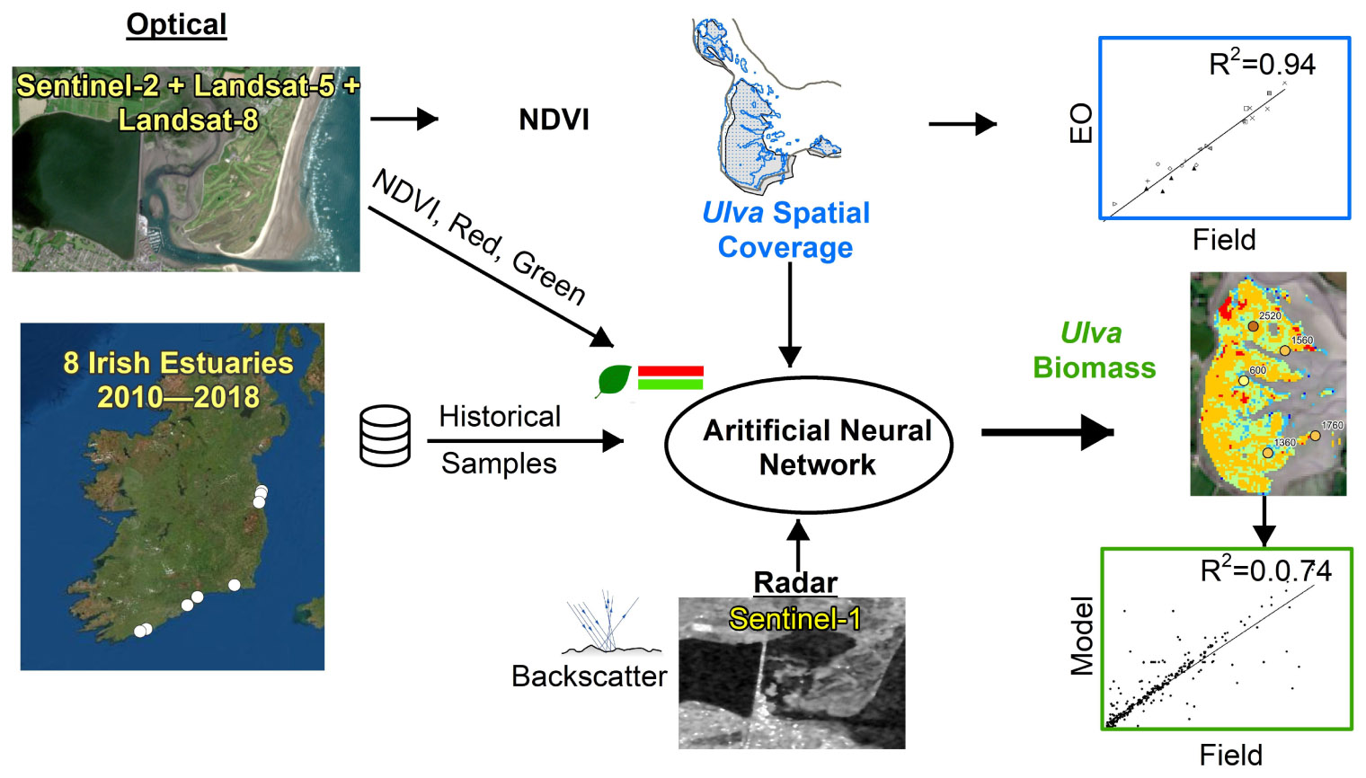
Graphical Abstract. Overall research workflow showing data types, study area, model development and biomass results.

Highlights

- Mapped green Ulva blooms across eight coastal areas of Ireland.

- Bloom extent mapped using Normalized Difference Vegetation Index delineation.

- Developed artificial neural networks (ANN) model to compute bloom biomass.

- The biomass model utilized optical, radar, and in situ data from field surveys.

- Developed technique could be used in conjunction with traditional monitoring.

Introduction

Estuarine and coastal areas play a crucial socio-economic, biological, and environmental role as these environments provide multiple ecosystem goods and services, making them some of the most valuable ecosystems on earth (Costanza et al., 1997; Donkersloot and Menzies, 2015; Norton et al., 2018). Due to their high value, these areas have been focal points of human settlement and resource exploitation (Lotze et al., 2006), resulting in a long history of over-exploitation, habitat transformation, and pollution. This legacy has undermined ecological resilience and has obscured the magnitude of degradation in estuarine and coastal environments (Lotze et al., 2006; Airoldi and Beck, 2007).

Estuarine and coastal waters worldwide have been facing the problem of eutrophication and macroalgal blooms (Teichberg et al., 2010). In Europe, eutrophication is considered one of the main threats for aquatic ecosystems (Airoldi and Beck, 2007; Hering et al., 2010). This process is directly linked with nutrient over-enrichment because of increasing anthropogenic nutrient loadings, which significantly increased after the generalized use of industrial fertilizers following the second world war (Cloern, 2001; Lotze et al., 2006; Diaz and Rosenberg, 2008). Due to the hydrological and ecological characteristics of estuaries, they are particularly susceptible to over-enrichment of nutrients and other pollutants from anthropogenic activities (Sfriso et al., 1992; Eyre and Ferguson, 2002). A clear sign of nutrient enrichment and environmental degradation in estuaries is the development of opportunistic macroalgal blooms and the loss of seagrass meadows (Valiela et al., 1997; Teichberg et al., 2010; Bermejo et al., 2019a). Considering the common usage of the terms, macroalgal bloom and seaweed tides, these are used interchangeably in the present paper.

Macroalgal blooms undermine the ecosystem services that estuaries provide, and affect ecosystem functioning (Smetacek and Zingone, 2013). As in other parts of the world, some Irish estuaries contained large green tides in recent years (EPA, 2006; Ní Longphuirt et al., 2016; Wan et al., 2017). A recent Environmental Protection Agency (EPA) report (EPA, 2019) has found that transitional waters (i.e., estuaries and coastal lagoons) in Ireland have poorer water quality when compared with other water typologies (i.e., groundwater, rivers, lakes, and coastal waters), with only 38% of water bodies in good or better ecological status.

The EU Water Framework Directive (WFD) 2000/60/EC (European Commission, 2000) and Marine Strategy Framework Directive (MSFD) (2008/56/EC; European Commission, 2008) are two of the most ambitious initiatives to prevent further deterioration of water bodies and associated ecosystems (Wan et al., 2017; Boon et al., 2020). These directives represent a change in the scope of water management from the local to the basin scale (Apitz et al., 2006). They are based on an ecological approach rather than a traditional physicochemical assessment (European Commission, 2000). This more recent approach is more holistic since it puts the ecosystem at the center of management decisions by considering ecology and biology at a larger scale (e.g., the whole river basin or adjacent coastal area) (Borja, 2005). Both directives require that coastal areas are periodically monitored to assess their achievement of “Good Ecological Status” and “Good Environmental Status” as per WFD and MFSD targets, respectively. The large expansion in monitoring required by the WFD and MFSD has created pressure from governments on their regulatory agencies to reduce the costs of monitoring while maintaining coverage and effectiveness (Borja and Elliott, 2013; Carvalho et al., 2019).

Marine macrophytes, including macroalgae and angiosperms such as saltmarsh and seagrass communities, are biological quality elements used to monitor and assess the ecological status of transitional and coastal waters for the WFD (e.g., Scanlan et al., 2007; Wells et al., 2007; Bermejo et al., 2012, 2013). Across the EU, monitoring of opportunistic macroalgal blooms is used to assess the ecological status (Scanlan et al., 2007; Wan et al., 2017), based on the relative coverage and biomass abundance of opportunistic macroalgae (Wilkes et al., 2018). Monitoring of coastal and estuarine environments can be demanding in terms of time, labor, costs, and sometimes can pose significant logistical challenges (European Commission, 2008) such as coordination of field equipment, survey procedures, means of transportation, field crew, and safety. The gathering of this information in muddy environments, especially the mapping of macroalgal blooms, can present several impediments as it frequently requires the use of specialized vehicles such as hovercrafts, or can be very labor intensive. Although these field surveys are systematic and provide high-quality data regarding spatial coverage and biomass, the cost of such works could range from medium to high (Scanlan et al., 2007).

Remote sensing can offer an affordable complementary solution to field-based environmental monitoring. Remote sensing data sets can be freely available, provide wide spatial and temporal coverage, and easily allow methodological standardizations and comparability. A conventional remote sensing technique such as aerial photography has been applied to map seagrass and macroalgal distribution in coastal and estuarine environments (Jeffrey et al., 1995; Hernandez-Cruz et al., 2006; Nezlin et al., 2007). Similarly, the application of earth observation (EO) satellite data to assess the severity and extension of algal blooms in coastal environments has grown in recent years (Cristina et al., 2015; Xing and Hu, 2016; Zhang et al., 2019). With the continued development of technology, unmanned aerial vehicles (UAV) are also being used to monitor green tides and seaweed blooms in marine environments (Xu F. et al., 2017; Bermejo et al., 2019b; Taddia et al., 2019; Jiang et al., 2020). Remote sensing methods have been shown to provide reasonable estimates of the algal coverage on the ground (Hernandez-Cruz et al., 2006; Nezlin et al., 2007), but with the availability of EO data sets with higher temporal, spatial, and spectral resolution, further improvement and development can be attained.

Different techniques such as image thresholding (Cavanaugh et al., 2010, 2011; Cui et al., 2012; Bell et al., 2015), visual interpretation (Donnellan and Foster, 1999; Gower et al., 2006; Pfister et al., 2017), supervised classification (Volent et al., 2007; Casal et al., 2011; Bermejo et al., 2020), and unsupervised classification (Fyfe et al., 1999; Duffy et al., 2018) have been used in vegetation mapping in coastal and estuarine areas. Among the thresholding techniques, band ratios, vegetation indices, density, and biomass are commonly used (Richards, 2013), whereas for supervised classification, spectral angle mapper and maximum likelihood classifications are more conventional approaches (Schroeder et al., 2019). Regarding classification, ground-truth data are used for supervised classification, whereas such information is not utilized for unsupervised classification. For both classification types, the results need to be validated with ground-truth data. Despite its simplicity, one of the disadvantages of supervised as well as the unsupervised classification is that it results in errors due to digital noise and these must be removed carefully (Schroeder et al., 2019). Unlike classification methods, the image threshold is determined based on the ground-truth data or a validation is performed to check the effectiveness of the threshold.

Many machine learning-based studies applying aerial or remote sensing imagery rely on the greenness of the imagery to map green tides. Although this technique is effective, some areas of the bloom could likely be underestimated, as the technique cannot easily delineate the bloom in its entirety. This unreliability results as the technique does not account for the spectral information available in the near-infrared (NIR) region where plants exhibit the majority of the photoactivity such as reflection (Tucker and Sellers, 1986). The Normalized Difference Vegetation Index (NDVI) is a proxy for vegetation health and greenness, and its value ranges from −1 to 1, where higher value corresponds to the healthy vegetation and lower values correspond to the lack of vegetation (D’Odorico et al., 2013; Ke et al., 2015; Zhu and Liu, 2015; Zhang H. K. et al., 2018). Since the NDVI technique uses the NIR bands, which are not visible to the naked eyes, it can detect the signature of vegetation that can go undetected when only visible green bands are used. Although there are numerous other vegetation indices (Silleos et al., 2006; Bannari et al., 2009; Xue and Su, 2017) used, including Enhanced Vegetation Index [EVI, primarily for Moderate Resolution Imaging Spectroradiometer (MODIS)], Maximum Chlorophyll Index [MCI, primarily for MEdium Resolution Imaging Spectrometer (MERIS)], and Floating Algae Index (FAI), NDVI was employed in the present study primarily because it incorporates the visible and NIR bands at 10 m resolution which are available in Sentinel-2. Additionally, indices developed for detecting vegetation or chlorophyll in aquatic conditions such as FAI and MCI are not applicable in the current context as macroalgal blooms are being mapped on tidal flats. Other studies (Siddiqui and Zaidi, 2016; Siddiqui et al., 2019; Taddia et al., 2019) have used NDVI and similar vegetation indices for mapping seaweed, but these studies mainly focused on seaweed immersed in the water. For the studies involving seaweed species in water, data sets from ocean color sensors have been used to obtain estimates of chlorophyll present in the water (Gower et al., 2006, 2008). Considering the size of the estuaries and the need to map these blooms at a higher spatial resolution, ocean color sensor-based techniques are not relevant to many estuaries globally. Recent studies have shown that NDVI can be successfully used for mapping biomass and density of intertidal macroalgae (Conser and Shanks, 2019; Praeger et al., 2020; Salarux and Kaewplang, 2020).

The assessments of the algal blooms are usually accomplished by comparing spatial coverage, but biomass can provide greater insights about the severity of the blooms (Scanlan et al., 2007; Rossi et al., 2011; Xiao et al., 2019). Furthermore, biomass results are more helpful for allocating resources and adopting mitigation measures. Despite the usefulness of biomass mapping, there are minimal studies that focus on mapping biomass using remote sensing data sets (Hu et al., 2017; Xiao et al., 2017, 2019). Most of these studies relied on reflectance computed in the laboratory environment in order to develop the biomass model. Those models were later used to generate biomass using the data from the MODIS optical sensor. Ocean color sensors such as MODIS are ineffective in mapping bloom patches that are smaller than a few hundred meters in size due to their coarse resolution of 500 m (Karki et al., 2018). Also, considering the spatial extent of the estuarine areas, it is essential to use remote sensing data with greater spatial resolution that can discriminate between various magnitudes of biomass on the tidal flats.

In addition to optical sensors, application of radar, for example, Advanced Land Observing Satellite-1 (ALOS) PALSAR for biomass estimation, at larger scales such as in forestry is common (Jha et al., 2006; Le Toan et al., 2011; Hame et al., 2013); however, its application can be explored at a finer scale for algal biomass estimation. In recent years, there have been many successful applications of Sentinel-1 technologies for biomass monitoring (Ndikumana et al., 2018; Periasamy, 2018; Crabbe et al., 2019) including those combining radar and optical data sets (Chang and Shoshany, 2016; Laurin et al., 2018; Navarro et al., 2019; Wang et al., 2019) or using radar for bloom forming Ulva species (Geng et al., 2020). The application of machine learning in the field of macroalgal blooms is increasing as demonstrated by recent studies (Zavalas et al., 2014; Kotta et al., 2018; Qiu et al., 2018; Liang et al., 2019; Kim et al., 2020).

Although the application of NDVI is conventional, the present study aims to optimize the benefit of NDVI combined with the application of radar and artificial neural networks (ANN) to predict the biomass of Ulva blooms. The benefit ANN offers over the traditional linear regression-type approach is the ability to model non-linear relationships (Huang, 2009; Karlaftis and Vlahogianni, 2011). An ANN offers the potential to deal with a large number of training samples and model complex relationships taking advantage of multiple input variables (Bourquin et al., 1998). Unlike other models, ANN offers the scope for future additional optimization, by the inclusion of more samples which in turn increases the robustness (Alwosheel et al., 2018). Therefore, the addition of more samples and the consideration of further variables provide a learning opportunity to the ANN model which improves predictability over time (Nadikattu, 2017). These neural networks when adequately trained can model the natural environment making them suitable to big-data applications such as remote sensing. Due to these scalable and expandable qualities, the ANN-based technique was adopted in the current study. Despite numerous benefits, there are some drawbacks of ANN which can be considered a “black box” because of its complex algorithms (Dayhoff and DeLeo, 2001; Zhang Z. et al., 2018). In addition, machine learning techniques require a comparatively large number of training samples, which may be difficult for smaller scale studies. More importantly, the requirement of robust computing and programming platforms frequently discourages quick and easy implementation.

The primary goal of the current study was to evaluate remote sensing as a supplementary tool for the monitoring of macroalgal blooms in Irish estuaries, where the presence of higher cloud coverage places an additional constraint. In this study, macroalgal bloom mapping based on satellite imagery was compared with in situ mapping for ground-truthing and validation purposes. The potential of machine learning methodologies was explored to map the biomass distribution since the higher resolution of the newer sensors, such as Sentinel-2 with 5-day revisit time and 10 m spatial resolution, accompanied by the greater size of the data, demands robust computing resources. The integration of these approaches in EO can take advantage of the recent technological advances in the field of data science and artificial intelligence (Ali et al., 2015). To address this challenge, the potential of an ANN was explored using the information extracted from Sentinel-1 radar backscatter and Sentinel-2 optical reflectance. The historical biomass data collected from field surveys were combined with the data obtained from the EO to develop the biomass model.

Materials and Methods

Study Area

The current research was conducted on eight estuarine areas most affected by macroalgal blooms across the Republic of Ireland (Figure 1): (a) Clonakilty, Co. Cork (3,465,900 m²); (b) Courtmacsherry, Co. Cork (4,471,200 m²); (c) Lower Blackwater Estuary, Co. Waterford (2,873,700 m²); (d) Dungarvan, Co. Waterford (12,399,300 m²); (e) Bannow Bay, Co. Wexford (9,848,700 m²); (f) Tolka, Co. Dublin (1,135,917 m²); (g) Malahide, Co. Dublin (4,075,200 m²); and (h) Rogerstown, Co. Dublin (4,488,300 m²). These areas show a moderate, poor, or bad ecological status as assessed for the WFD, parameters driving status included loss of seagrass meadows, general physico-chemical properties, or the development of large macroalgal blooms (EPA, 2019¹). Although there were different numbers of estuaries in each category (moderate: 4; poor: 3; and bad: 1), standard field surveying techniques were conducted regardless of their status. Consistent with the field protocol, identical EO mapping techniques were also applied. It was important to include a varied range of ecological status conditions in this study to make sure that the proposed technique for mapping blooms was not limited to a narrow set of environmental conditions.

FIGURE 1

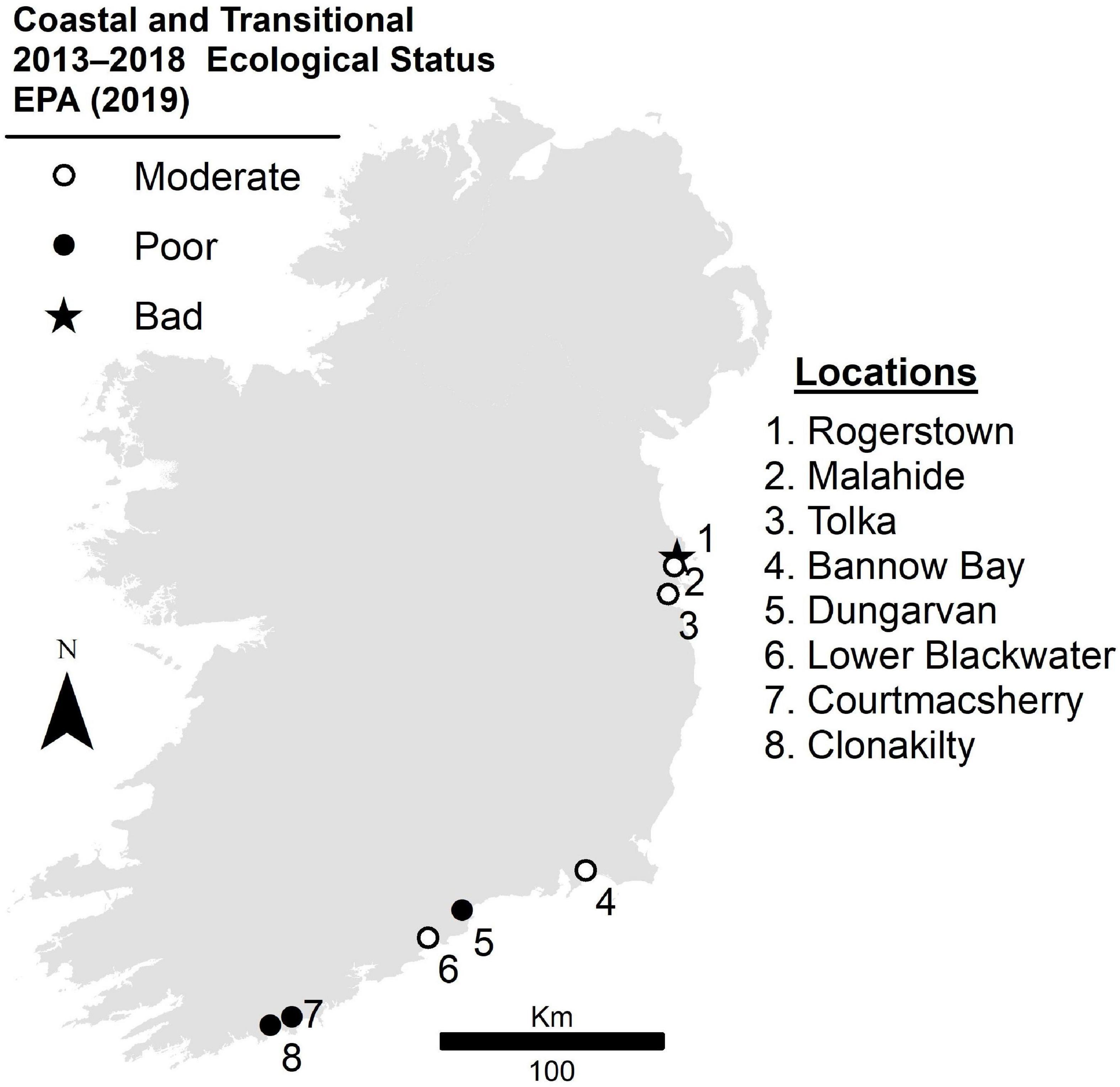
Figure 1. Map of Ireland showing eight estuarine areas considered in this study with their ecological status based on the study conducted from 2013 to 2018 (EPA, 2019).

In this study, seaweed blooms resembling terrestrial vegetation present in the estuaries and tidal flats, excluding the salt marshes, were mapped during the low tides. These algal patches must be mapped during the low tide condition when there is no water above them. It is crucial to note that estuaries in Ireland are intertidal in nature, and blooms present in the tidal flat region may not have water above them except during high tide conditions. In six of the eight sampling locations, seagrass meadows were absent, or their presence was negligible (i.e., Clonakilty), and only Bannow Bay had conspicuous seagrass meadows present. Bannow Bay primarily includes intertidal zones with predominant macroalgal growth, and the distinction between seagrasses and Ulva was not conducted because of the interspersed, or sometimes negligible, growth of seagrasses among the macroalgal blooms. Apart from the practical reasons, green algae and seagrasses are difficult to separate from each other at the current spectral and spatial signature (Kutser et al., 2020). Since the discrimination between seagrasses and macroalgae is not possible with Sentinel-2, the study aims to develop a methodology so that field validation can be performed where substantial levels of macroalgal growth occur and any potential false positive incidences due to the presence of seagrasses can be verified. This is an example of field monitoring and EO complementing each other, reducing logistical and human resource costs, and enhancing environmental quality assessment. Seagrasses in Bannow Bay are routinely monitored and mapped as a part of obligations under the WFD and the data confirm no risk of false observations from the EO mapping.

Field Survey

In Ireland, as well as in other cold-temperate regions, the maximum development or peak of macroalgal blooms occurs during the summer (Jeffrey et al., 1995; Bermejo et al., 2019a, 2020). For this reason, the monitoring of the estuaries and the field sampling were concentrated through late June to early October. The current study focused on blooms from 2010 to 2018, because of the lack of overlap between field surveys and Landsat acquisitions prior to that date.

Bloom extension and biomass abundance were obtained from the WFD surveys conducted by the EPA to assess the ecological status of opportunistic algae blooms on the dates shown in Table 1. The table shows the dates and locations for which both field spatial coverage and biomass data sets were available and were collected as a part of the WFD monitoring. Since the WFD method primarily focuses on surveying of algal mats that are mostly attached, spatial coverage and algal biomass were assessed in situ. The outer edges of the algal accumulations were mapped at low tide using a mapping grade Global Positioning System (GPS) unit with accuracy of a meter. A light hovercraft was used in areas where the sediment was too soft to allow safe access or where the algal beds were too large to allow safe mapping during a single tidal cycle (Wilkes et al., 2017). A series of transects were taken through each patch and haphazardly distributed 0.5 m² quadrants were taken along each transect, and their GPS locations were recorded. The percentage cover and algal biomass in each quadrant were recorded. Biomass from each quadrant was collected, washed, and rinsed in fresh seawater to remove sand and debris, squeezed dry, and the weight recorded as g/m² wet weight. The data were compiled into five sub-metrics (i.e., total percentage cover, total patch size as a percentage of available intertidal habitat, average biomass on the intertidal area, average biomass in affected area, and percentage of quadrants with algae entrained into sediments) to provide a WFD assessment for the estuaries (Scanlan et al., 2007; Wan et al., 2017). To meet the requirement for sufficient training data for model development, additional data collected as a part of the Sea-MAT Project (Bermejo et al., 2019b), not shown in Table 1, were used. This biomass abundance (g/m²) data, collected between June 2016 and August 2017 following a similar methodology, were exclusively used for ANN training and validation.

TABLE 1

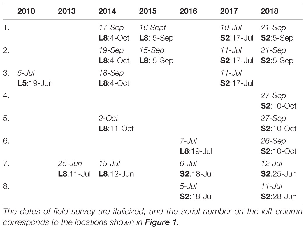
Table 1. Dates of the field investigation and corresponding source of EO data sets: Landsat-5 TM (L5), Landsat-8 OLI (L8), or Sentinel-2 MSI (S2) missions.

Earth Observation Mapping of the Spatial Coverage

The mapping of macroalgal blooms using satellite imagery comprises several steps starting from data download to the generation of the map (Figure 2). The study utilizes the EO data sets from the Sentinel-2 and Landsat (5 and 8) missions to acquire the temporal coverage from 2010 to 2018. The Landsat mission from the National Aeronautics and Space Administration (NASA) has been operational since 1972, although the availability of free and open-source data is a more recent practice that started in 2008 (Zhu et al., 2019). To get better temporal coverage from 2010, data sets from Landsat-5 Thematic Mapper (TM; data availability:1984--2012) and Landsat-8 Operational Land Imager (OLI; data availability: 2013--2018) were used. The data sets are freely available from the United States Geological Survey (USGS)’s Earth Explorer².

FIGURE 2

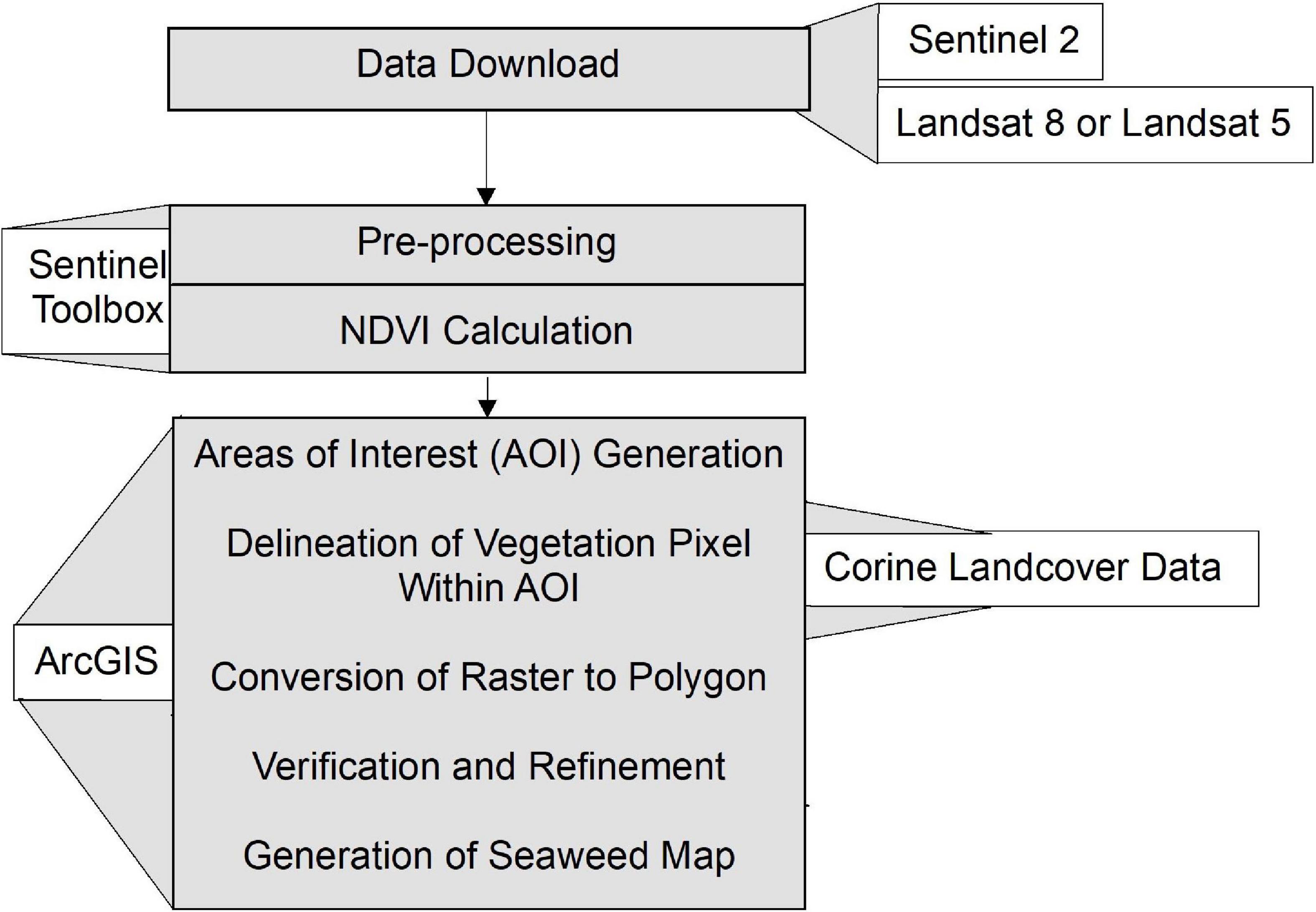
Figure 2. The workflow developed for mapping blooms using the NDVI delineation technique.

Both, Landsat-5 and Landsat-8 missions provide the images with a swath width of 185 km and a temporal resolution of 16 days (USGS, 2020). These missions are identical from the application and data processing point of view, especially for the bands being considered for this study. Landsat bands in the visible region (red, green, and blue) and NIR are available at 30 × 30 m resolution. Unlike Landsat missions, Sentinel-2 Multispectral Instrument (MSI), under European Space Agency (ESA)’s Copernicus Program, is the newest EO mission and provides the acquisitions since 2015. It consists of the constellation of Sentinel-2A and 2B MSI sensors with a combined revisit time of 5 days at the equator and swath coverage of 290 km (ESA, 2019). The bands required for natural color (red, green, and blue) imagery and vegetation mapping (red and NIR) are available at 10 × 10 m resolution. These data sets are available freely from ESA’s Sentinel Hub³.

Data Acquisition

The identification of the dates was based on the availability of the field survey data collected from 2010 to 2018 as a part of the WFD monitoring program. In response to the number of field data accompanied by the need to find matching EO scenes with low tide and cloud-free conditions, images acquired either before or after the field surveys were indiscriminately considered for the study. This is considered the accepted practice in the field of remote sensing and is unlikely to affect the outcome of the study for mapping Ulva blooms. For each location, the archival Sentinel-2 data were screened for cloud-free scenes within two and half weeks of the field monitoring program under conditions of low tide. In the absence of Sentinel-2 MSI scenes (10 m resolution, 2015–2018), Landsat-8 OLI (30 m resolution, 2013–2018) scenes were used. For scenes prior to 2013 (2010–2012), Landsat-5 TM (30 m resolution; 1984–2012) images were used. Table 1 provides the detailed information about the field survey and corresponding source of EO data sets for each of the eight locations. Considering the small number of historical WFD monitoring data with associated geospatial information followed by the difficulty in finding corresponding EO scenes, data from 2010 were selected despite the fact that there were no matching scenes for the two subsequent years (2011 and 2012). Additionally, 2010 is the only year for which Landsat-5 data were used, which is identical to Landsat-8 from the application point of view. Thus, the inclusion of 2010 despite a gap of two years and the usage of Landsat-5 was important for this study. Sentinel-2 Level 2A (atmospheric corrected) products covering the areas under consideration were identified and downloaded from ESA’s Sentinel Hub website. Similarly, Level 2 Landsat-5 TM and Landsat-8 OLI products were downloaded from the USGS Earth Explorer’s website.

Pre-processing

The second step involved pre-processing of the scene in order to reduce the size of the files to allow quick processing in freely available Sentinel Application Platform (SNAP) software from ESA. In the case of Sentinel-2, pre-processing was accomplished as a first step to resize the entire image to the resolution of 10 m bands (either blue, green, red, or NIR). This step helped to synchronize all the coarser bands (20 and 60 m) to a resolution of 10 m. This is the most essential step before doing spatial and spectral sub-setting since it helps to significantly reduce the computing time. After resampling, each scene was resized and clipped to the extent of each location under investigation. During the same step, the spectral sub-setting was completed to retain the specific bands required for further processing (blue, green, red, and NIR). In the case of Landsat-5 and Landsat-8, the scene was resampled to the extent of 30 m band prior to spatial and spectral sub-setting.

NDVI Calculation

Although several remote sensing indices are in use for vegetation mapping, NDVI is the most widely used index (Xue and Su, 2017). The method used in this study is based on the NDVI for mapping and delineating the bloom. It utilizes the characteristic increased reflectance in the NIR region and decreased reflectance in the red regions of the electromagnetic spectrum exhibited by the vegetation (Jensen, 1986; Tucker and Sellers, 1986). The NDVI is calculated using Eq. 1.

$$\text{NDVI}=\frac{(\text{NIR}-\text{Red})}{(\text{NIR}+\text{Red})}(1)$$

The next step was to compute NDVI using red and NIR bands in SNAP software. During the band specification, corresponding bands were identified for Sentinel-2, Landsat-8, and Landsat-5. All the processing after this step was done using ArcGIS software and Python 2.7. Since NDVI computation involves the uses of NIR band, it can overestimate the bloom coverage by including microphytobenthos present in the sediment that contributes to the primary production in an estuarine environment (Launeau et al., 2018). To prevent this risk, the results from NDVI needed to be verified with field data. One important advantage of using NDVI was its ability to detect live vegetation, due to the consideration of NIR reflectance exhibited only by photosynthetically active plants.

Generation of Algal Bloom Map

The Corine (Coordination of Information on the Environment) land cover data set⁴ was used to define area of interest (AOI, i.e., intertidal mudflats) for each location. Following Corine land cover classification, the classes of interest corresponded with the tidal flats (4.2.3) and estuaries (5.2.2) labels. This facilitated the removal of terrestrial vegetation and saltmarshes from the consideration.

The visual inspection was done to determine the threshold of the NDVI values that corresponded with the bloom-forming seaweed in the natural color composite. In most cases, NDVI values greater than 0.15 and 0.20 for Sentinel-2 and Landsat images, respectively, represented Ulva blooms. For each location, the vegetation pixels were segregated after determining the threshold. This technique was able to segregate bloom patches bigger than a few meters.

Manual verification, subjective judgment, and refinements are essential steps of the mapping workflow to assure that the bloom pixels are represented correctly. Spatial delineation of the macroalgal blooms using the NDVI technique was the initial step, and subsequently the computation of biomass relied on the spatial extent outlined. Correct spatial delineation ensured that healthy Ulva tissue, as opposed to decomposing tissue, was only considered. In specific locations, it was necessary to eliminate areas which corresponded to terrestrial vegetation. Due to the coarse resolution of Corine land cover data sets, a few areas also included artificial structures and salt marshes. The minimum mapping area for Corine land cover data sets is 50,000 m² for land cover change and 100 m for linear units. For features smaller than these minimum mapping units, a generalized class is reported in the Corine database. Because of such boundary generalizations for small features, these areas were carefully clipped out from the AOI polygons. The final step involved the generation of the vector and raster outline of the algal blooms for all locations. The area of the bloom was computed, and the percentage coverage was calculated by taking into account the AOI of each site under consideration using the following Eq. 2.

$$\text{Percentage}\text{Cover}=\frac{\mathrm{Area}\mathrm{delineated}\mathrm{by}\mathrm{NDVI}\mathrm{technique}\mathrm{in}\mathrm{the}\mathrm{AOI}}{\text{AOI}}\times 100(2)$$

Validation and Statistical Analysis

To test the comparability and consistency of macroalgal blooms mapping using satellite imagery and field surveys, and to identify possible disagreement between methodologies, Pearson correlation analyses and paired t-tests (Xu M. et al., 2017) and Cohen’s kappa analyses were conducted. The limited number of samples for Landsat show marginal significance compared to other groups, whereas Sentinel with native bands shows higher significance. Similarly, the root-mean-square error (RMSE) was calculated to examine the error where lower value indicated better estimates. Similarly, to assess the influence of the temporal gaps between field surveys and satellite images, the correlation between relative mismatches and the time lapse between samplings was evaluated. All statistical analyses were performed using Minitab software, ArcGIS, and Python packages. When necessary Shapiro–Wilks and Levene’s tests were used to ensure compliance with normality and homoscedasticity assumptions. In all statistical analysis, significance was set at 5% risk error.

The time gap between the EO data acquisition and field survey varied from same day to a maximum of 18 days (+/−) with an average of 12 days for 22 pairs of observations. Out of those 22 observations, 12 were Sentinel-2 and 10 were Landsat acquisitions, as we primarily focused on finding Sentinel scenes and selected Landsat only when the former was not available. Since it was not possible to obtain both Sentinel and Landsat scenes for each location for the same date during the scene selection, more direct comparison between the influences of resolutions on identical conditions was not possible. To address this, the Sentinel bands were resampled to 30 m in order to compare the findings from the 10 m Sentinel-2 bands. This helped to compare the overall effects of resolution on the estimated coverage at the same location with fine and coarse pixels on the same day. Further, the upscaling of the Sentinel bands to 30 m facilitated the comparison with original Landsat bands.

Computation of Algal Biomass Using Machine Learning

Building upon the spatial coverage extracted using the NDVI delineation approach, an ANN model was developed to quantify the biomass distribution in the estuarine area. Sentinel-1 Synthetic Aperture Radar (SAR) and Sentinel-2 MSI were used to develop the ANN model. The in situ biomass samples (point locations in g/m²) collected as a part of WFD monitoring program and those obtained under Sea-MAT project (Bermejo et al., 2019b) were compiled as a response variable for the model. The entire biomass computation process can be broken down into data acquisition and processing, identification of determining variables, model development, and application, as shown in Figure 3.

FIGURE 3

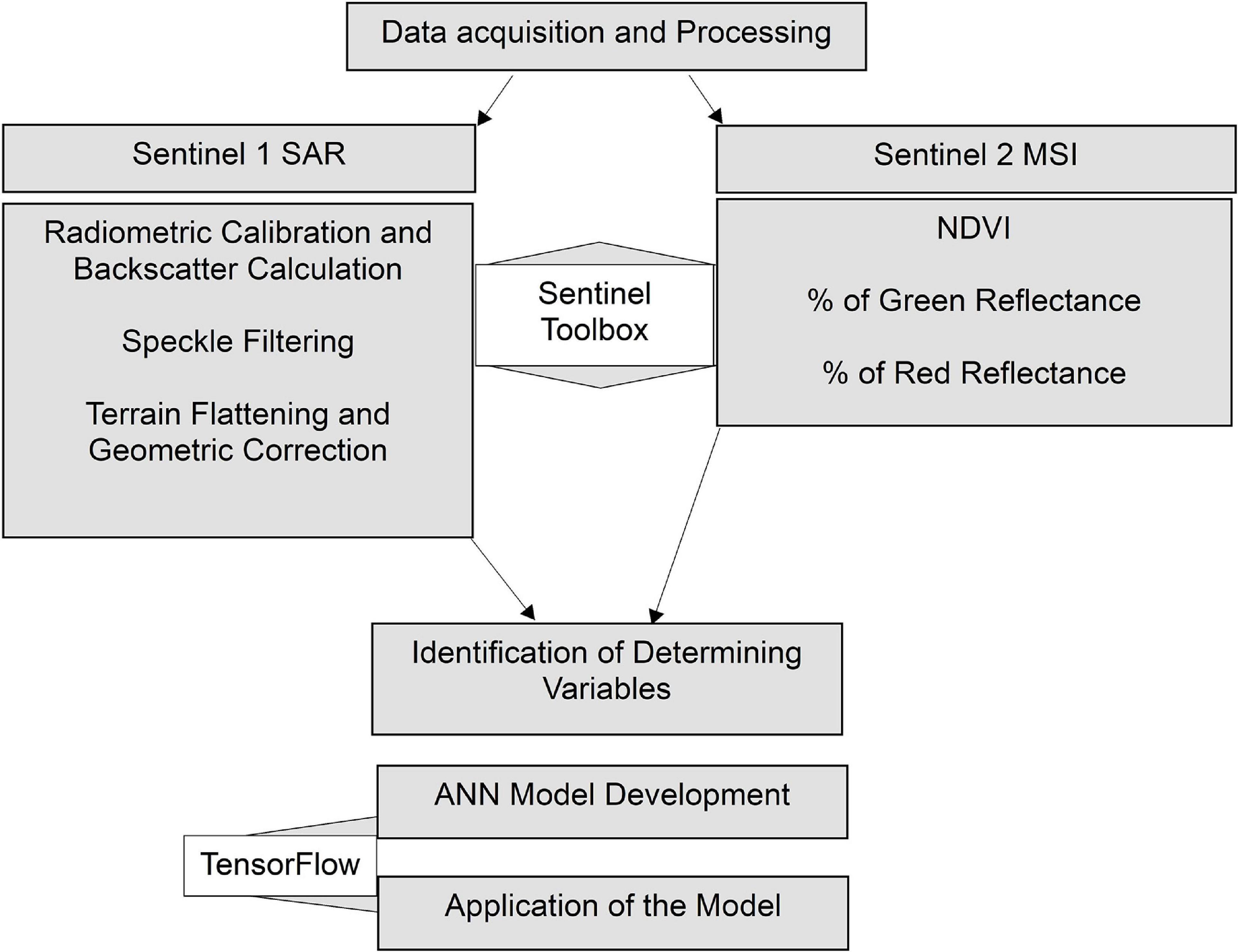
Figure 3. The workflow developed for computing biomass using ANN.

Data Acquisition and Processing

Sentinel-2 scenes acquired for mapping spatial coverage of Ulva blooms were also used for biomass calculation. In addition to NDVI, two more products, percentages of green and red reflectance, were calculated using visible and NIR bands. Altogether 11 Sentinel-2 scenes corresponding to biomass surveys were used for computing optical variables. Apart from optical data, Sentinel-1 SAR scenes, acquired from ESA’s site, provide the radar information in C-band at a spatial resolution of around 10 m. Sentinel-1 images were acquired in either ascending or descending modes covering the study area. The standard radar data processing chain (Small and Schubert, 2008; Small, 2011; Veci, 2016; Filipponi, 2019) were followed using ESA’s Sentinel Toolbox. The processing steps include:(i) radiometric calibration and calculation of radar backscatter; (ii) speckle filtering; and (iii) terrain flattening and geometric correction. The final product of the processing was radar backscatter in decibels (Raney et al., 1994). Sentinel-1 SAR is dual polarized, capable of HH/HV and VH/VV acquisition, but VH/VV is the default mode. Polarization can impact on the results, and cross-polarized (VH) data were found to provide better results. Altogether 16 radar scenes corresponding to the biomass field survey data were processed which were acquired within 5 days of the data collection. In addition to satellite derived variables at the resolution of around 10 m, biomass data collected at the field resolution of 0.5 via field survey were used in the study.

Identification of Determining Variables

The independent variables were identified, which would explain the variability of biomass in the study area. At first, all the potential variables that could be related to biomass were considered. Among such variables, NDVI, percentage reflectance in green, red, and infrared wavelengths were selected as determining variables. Similarly, radar backscatter was considered as one of the determining variables since it is the measure of surface roughness. The test of significance and redundancy was carried out using variance inflation factor (VIF) analysis (O’Brien, 2007) through correlation before selecting the independent variables, and only four variables were shortlisted for inclusion in the model training because these were found significant as well as non-redundant. Inclusion of these additional variables for their non-linear contribution is expected to prevent the potential saturation of NDVI at higher biomass values (Huete et al., 2002; Garroutte et al., 2016; Xiao et al., 2017).

Development of the Model

An ANN models the relationship between the dependent and independent variables with the help of training and validation data. The model consists of multiple inputs, activation functions, hidden layers, and an output which are connected via artificial neurons and transmit information through structured layers (Dayhoff and DeLeo, 2001). These interconnected neurons work exactly like the neurons present in the nervous system of organisms where it learns the relationship among input variables through multiple iterations or epochs (Zurada, 1992; Agatonovic-Kustrin and Beresford, 2000; Hu et al., 2018). An ANN consists of different combinations of input variables with associated empirical weights and bias terms (Huang, 2009). Backpropagation is one of the techniques where parameters such as the number of inputs, bias terms, and weights are adjusted in forward and backward fashion until the minimum error is achieved (Rumelhart et al., 1986; Aggarwal, 2018; Hu et al., 2018). The model training and, hence hyperparameter tuning, is attained in several iterations until a stable solution is achieved. With each iteration of the ANN model, these configurations are tuned so that the structured layers of neurons can model the expected output (Bardenet et al., 2013). During the ANN development, a small number of validation data sets are set aside to prevent overfitting (Shahin et al., 2005; Piotrowski and Napiorkowski, 2013). This step assures that the model is generalized enough, and its robustness does not degrade outside of the training samples. Thus, during the model training, the samples should be representative so that the neurons can learn to model the complex relationships adequately and appropriately.

The ANN model was developed using the total of 346 biomass samples where the magnitude of biomass (g/m²) was the response variable, and remaining variables (NDVI, percentage of green reflectance, percentage of red reflectance, and radar backscatter) were used as determining variables. Out of the total samples, 20% of the data points were used as validation data, where these prevent the model from overfitting due to excessive training. The hyperparameters, such as the number of hidden layers and the number of iterations to achieve a stable solution, were determined based on the error statistics reported by the model by using backpropagation-based learning algorithms (Huang, 2009). The fully trained ANN model was achieved with five hidden neurons when the number of epochs reached 50. The learning process was continued until the model performance plateaued where the error was minimal for both validation (20%) as well as training (80%) data sets. The entire process was accomplished using Google’s TensorFlow (Abadi et al., 2016), a free and open-source application using Python programming language. The input data preparation was done using ArcGIS, where a table consisting of all input variables was generated.

Application of the Model

After the development of the model, the ANN model was applied to generate the biomass values using the input variables. In order to apply the model, the input data sets were extracted and compiled in the form of a table. The TensorFlow generated results were later converted to geographic information system (GIS) raster for mapping and further analysis. The biomass quantity can be predicted for any area as long as input data sets are available for any area.

Results

Spatial Coverage of the Bloom

The extension of the macroalgal blooms from field surveys ranged between 213,100 and 5,425,900 m² for Lower Blackwater Estuary (2017) and Tolka (2017), respectively. There was a total of 22 EO estimates with corresponding field survey data, some of which are shown in Figure 4. A significant correlation between EO estimate and survey measurements was observed, which was independent of the satellite missions used (p-values < 0.01). All the correlation analyses yielded coefficients of determination close to 1 (between 0.93 and 0.98) and a good fit between the observations (Figure 5). The spatial coverages from EO show more detailed delineation than those mapped on the ground since the field campaign was more concentrated on the predominant and accessible regions of the Ulva blooms. The scatter plots for all the observations made for eight estuaries using Sentinel-2 and Landsat are presented in Figure 5 together with R² value, slope, and intercept for each plot.

FIGURE 4

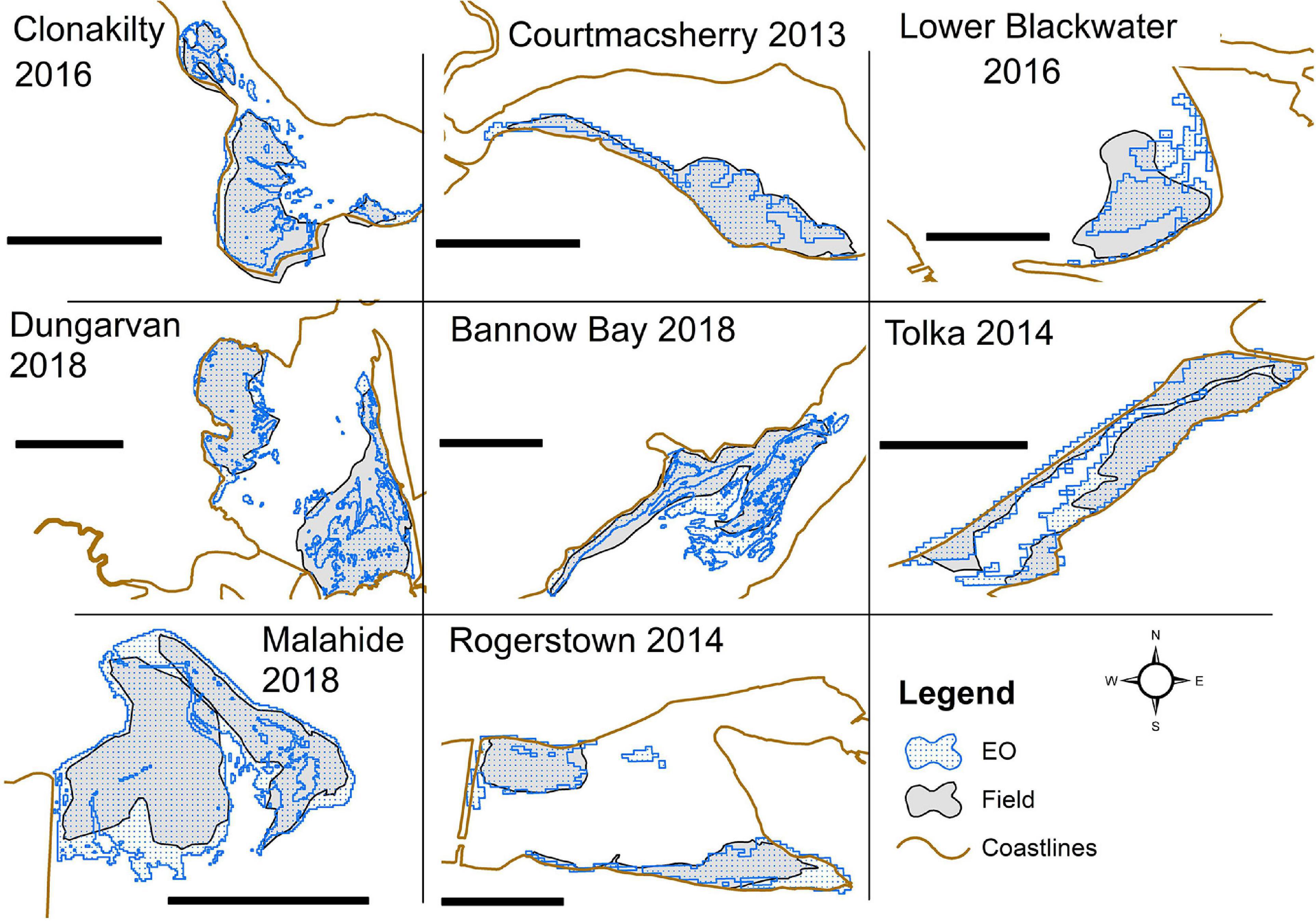
Figure 4. Eight locations showing selected sites with coverages from EO and the corresponding field surveys. Scale bar shows 1 km in all the locations.

FIGURE 5

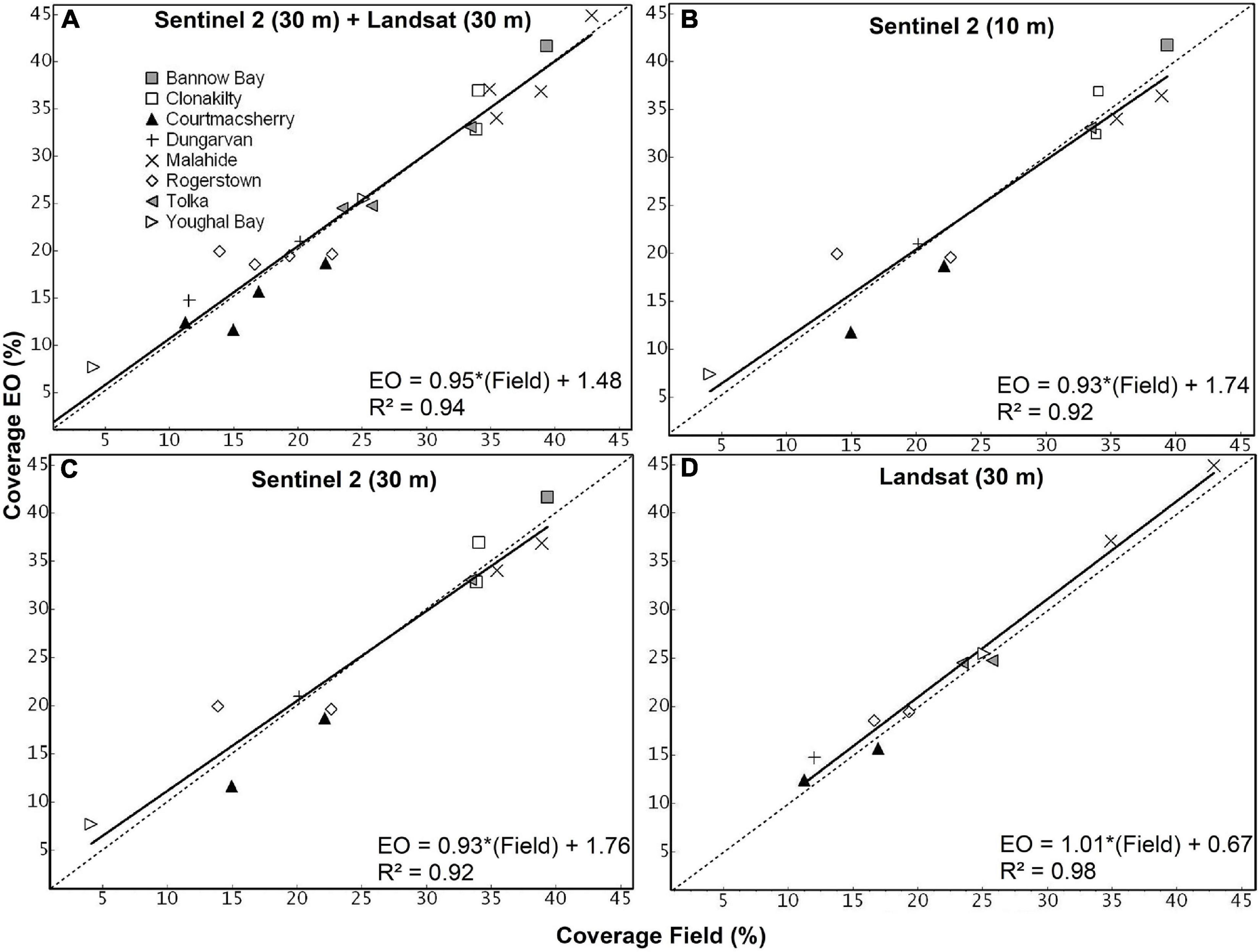
Figure 5. Scatterplots showing the comparison between coverage computed using the EO and coverage obtained using the field survey for four groups based on the resolutions of the EO data sets: (A) resampled Sentinel-2 30 m and Landsat 30 m, (B) Sentinel-2 10 m, (C) resampled Sentinel-2 30 m, and (D) Landsat 30 m. The equation of the trend line, the associated R² values have been shown for each plot. The 45° line with 1:1 correspondence between EO and field data has been shown as a dotted line for reference.

Although resampled Sentinel-2 bands, upscaled to 30 m, are a derivative of bands acquired originally at 10 m resolution, it provided a similar level of performance in terms of delineation of the green algal blooms and one-to-one correspondence with the field data. The EO data sets show a slight overestimation compared with the field data, as shown in Figure 5. This overestimation is slightly higher in Figures 5B,C which corresponds to Sentinel-2 original and resampled products, respectively. For each scatter plot, the equation of the trend line shows the magnitude of the bias, and the slope of the trend line shows the level of estimation (over or under) between EO and field survey. Comparing the rate of over- and underestimation, Landsat seems to be consistent, although exhibiting a slight overestimation as indicated by the upward shift of the trend line compared to the 1:1 dotted line. Sentinel-2, in contrast, shows overestimation for lower magnitudes and a slight underestimation for higher magnitudes of coverage. These under- and overestimations of Sentinel-2 and Landsat imagery seem to be compensating each other on the combined scatter plot in Figure 5A. The slope of the regression lines (Figure 5) was close to 1 for all correlation analyses, and the results of the paired t-test (Figure 6 and Table 2) suggest no methodological bias. The p-value for all groups of observations shows values higher than 0.05, as shown in Table 2. Overall, there was no bias as can be seen from Figure 5 and suggested by the paired t-test.

FIGURE 6

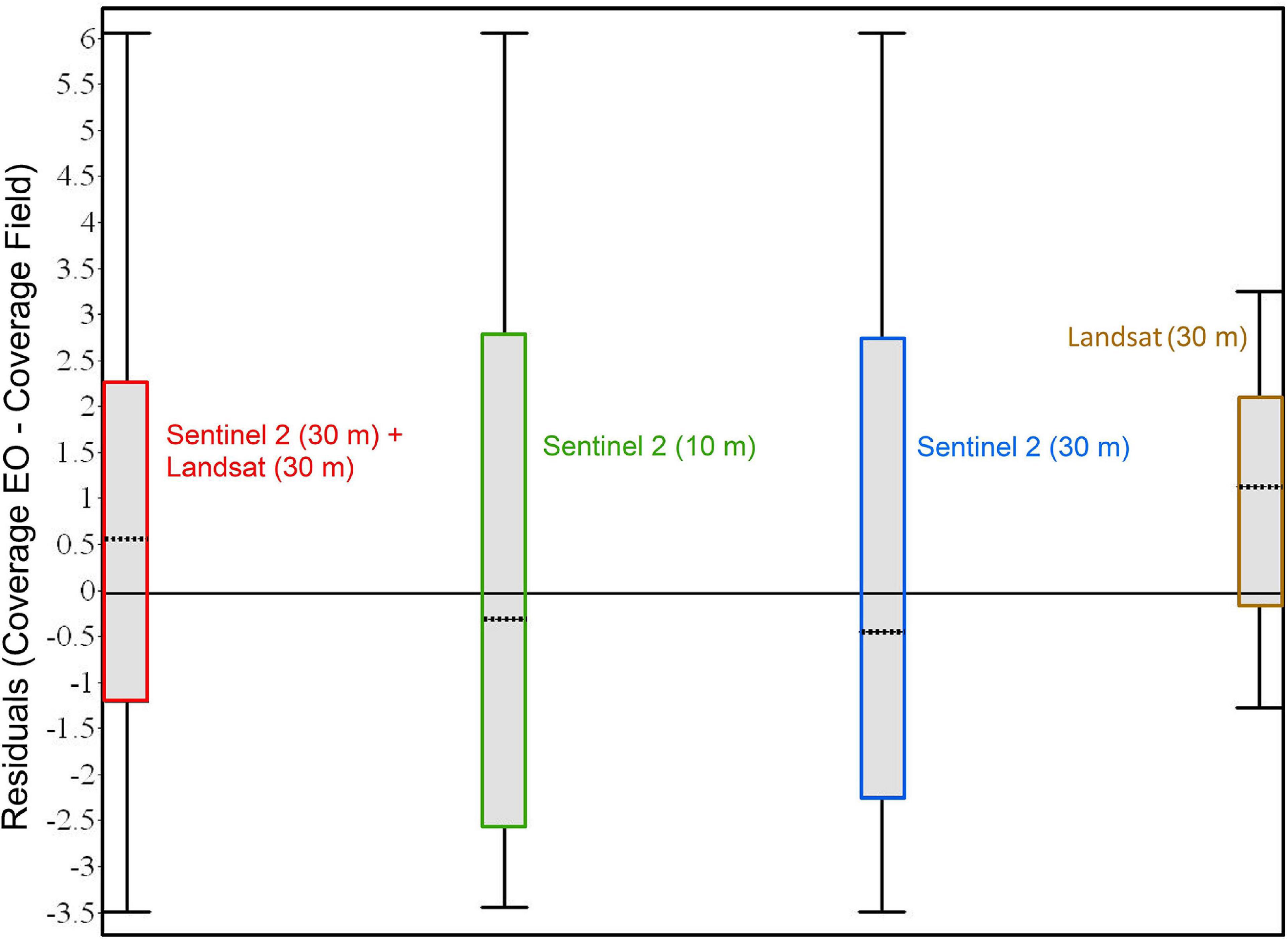
Figure 6. The box plots showing the residuals computed between the EO estimates and field coverages. The upper and lower bounds of the box represent the first and third quartiles, whereas the dotted line represents the median. The long horizontal line shows the zero value. The whisker shows the range of the residual data.

TABLE 2

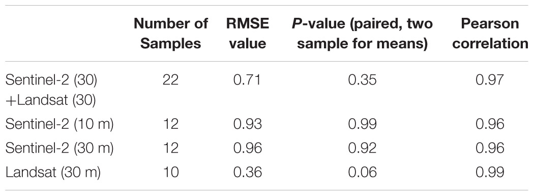
Table 2. Results of the two-sample paired t-test for EO estimates and field measurements.

Regarding the error statistics, the result of the t-test shows that the RMSE is lowest for Landsat, followed by the RMSE for the combination of resampled Sentinel-2 and native Landsat bands at 30 m. The Pearson correlation showed the correlation between EO estimates and field measurements, where Landsat shows the best results followed by the combination of Sentinel-2 and Landsat observations. Based on the RMSE and Pearson correlation values, the Landsat appears to have performed better than Sentinel with finer resolution. Nevertheless, the low number of observations for Landsat may not statistically prove that it is performing better than the Sentinel. Overall, the results show that native Sentinel-2 bands perform better than resampled bands, as evidenced by lower RMSE. In addition, the resampled Sentinel-2 still managed to provide better results and did not offer significantly higher error than the native bands.

The error analysis was done by comparing the distribution of the residuals computed between the EO estimates and the field survey data. After these inter-comparisons of the residuals, it is equally important to see if there was any notable correlation between the difference/discrepancies in percent coverage (EO estimates and field measurements) with the corresponding time lag between them. Thus, the relationship between the differences in percent coverage was analyzed against the time lags. Figure 6 shows the differences in bloom coverage estimated using EO and field surveys. From the magnitude of the residuals, it is evident that the differences cannot be considered different to zero in all the cases except marginal difference in the case of Landsat. With very few observations for less than 1 week and more than 2 weeks, it was difficult to draw any conclusion about the magnitude of the effect due to the time gap. Figure 7 shows the number of days between those observations and the absolute difference between the percentage coverages. The individual breakdown of Cohen’s kappa for each Sentinel-2 and Landsat observation is indicated by its label and color code. This figure aids visualization of the distribution of data in relation to Cohen’s kappa which highlights the measure of agreement between field and EO estimations. Cohen’s kappa value also provides important information about changes in the position of the bloom or the degree of spatial agreement between EO and field data. Most of the observations clustered around 10–13 days without showing any trend with the difference in the percentage coverage or Cohen’s kappa (Figure 7), and the Pearson correlation coefficient indicated no correlation (Pearson’s r < 0.01) between them.

FIGURE 7

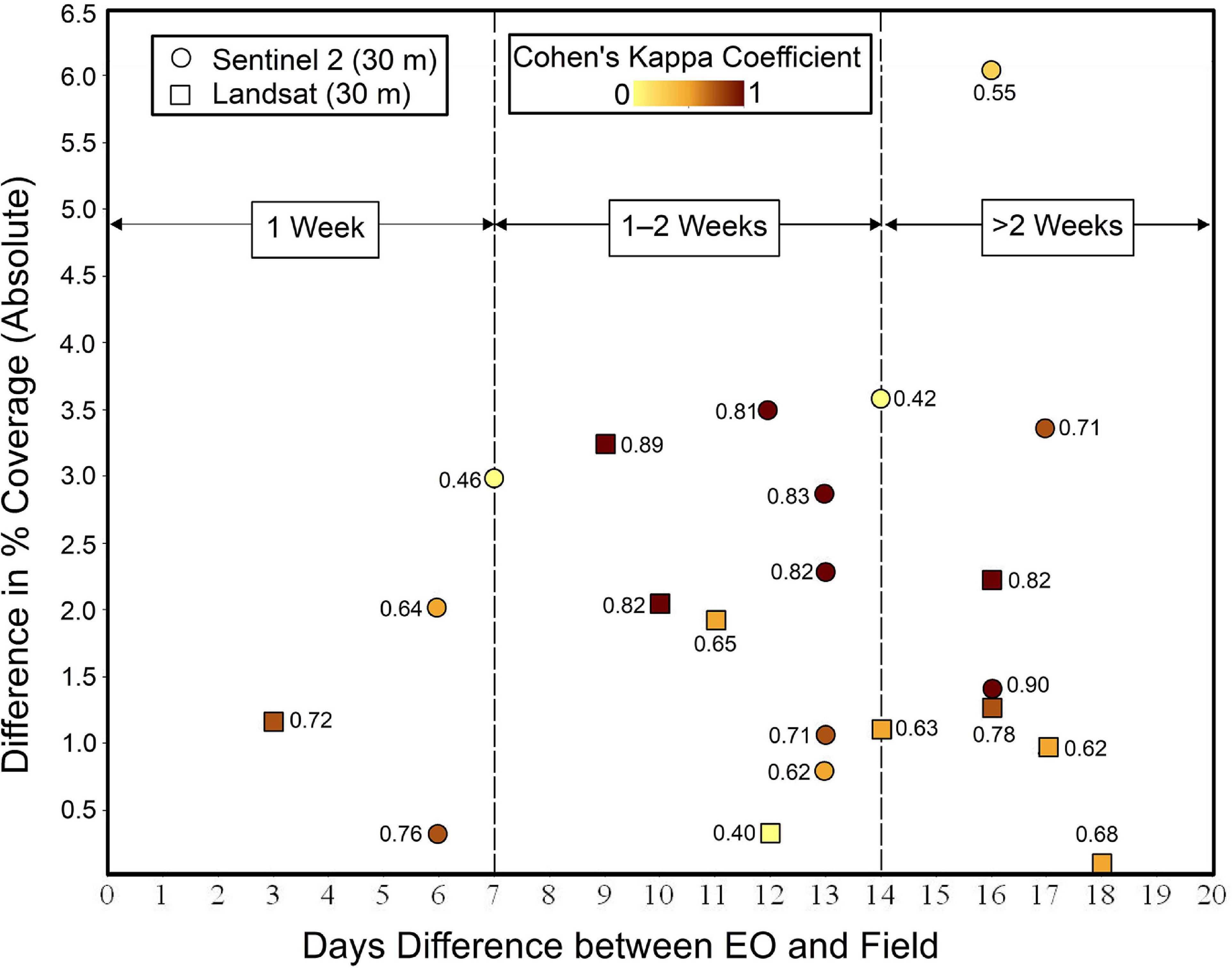
Figure 7. The scatter plot for the time gap between EO and field surveys versus the difference in percentage coverage. The number next to each observation and the intensity of color represent Cohen’s kappa coefficient and its magnitude.

Biomass Computation of the Algal Blooms

The ANN model was developed by using NDVI, percentages of green and red reflectance, and radar backscatter to compute the biomass in g/m². Only the non-redundant and significant variables were used in the ANN model development based on the result from the redundancy test using VIF (O’Brien, 2007) and correlation analysis. Figure 8 shows the scatter plots of biomass with each of the determining variables where the correlation with red reflectance was highest, followed by NDVI, green reflectance, and the radar backscatter. The predicted result was compared with the biomass data measured from the field survey with RMSE value of 471.70 and adjusted R² of 0.74, as shown in Figure 8E.

FIGURE 8

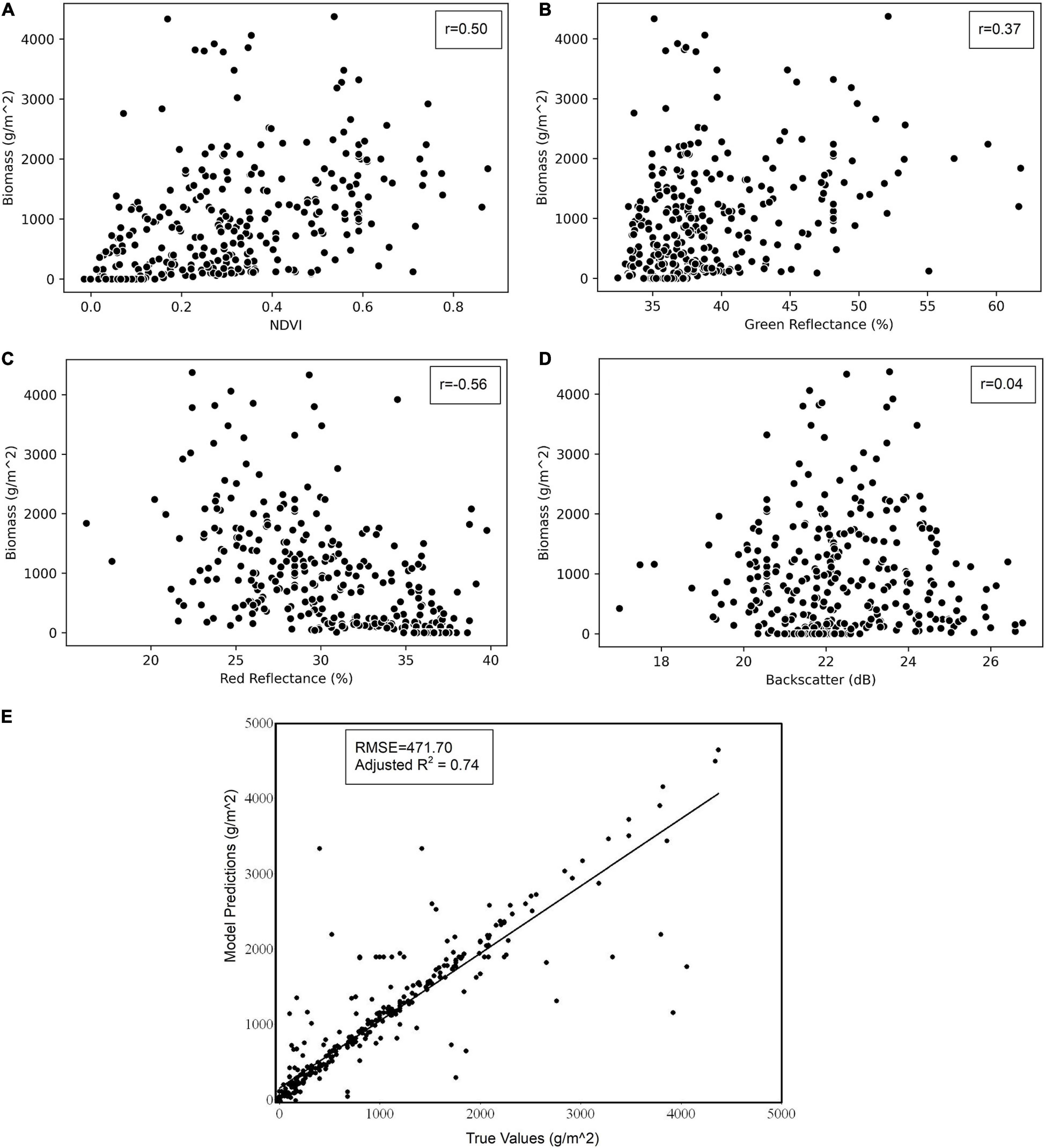
Figure 8. Scatterplots showing the correlation between biomass data from field surveys and other determining variables: (A) NDVI, (B) green reflectance, (C) red reflectance, and (D) radar backscatter. Scatterplot on the bottom (E) shows the field survey biomass data versus the predicted biomass from the ANN model.

The ANN model was used to compute the biomass images for several estuarine areas. The biomass image shows the distribution of biomass blooms within the areas delineated by the spatial coverage mapping technique based on NDVI. Figure 9 shows the biomass distribution where both the EO scenes acquisition and the field survey were conducted in the summer of 2016 and 2018 for Clonakilty (Figure 9A) and Courtmacsherry (Figure 9B), respectively. Similarly, the computed biomasses for Malahide and Tolka for the summer of 2017 are shown in Figures 9C,D, respectively.

FIGURE 9

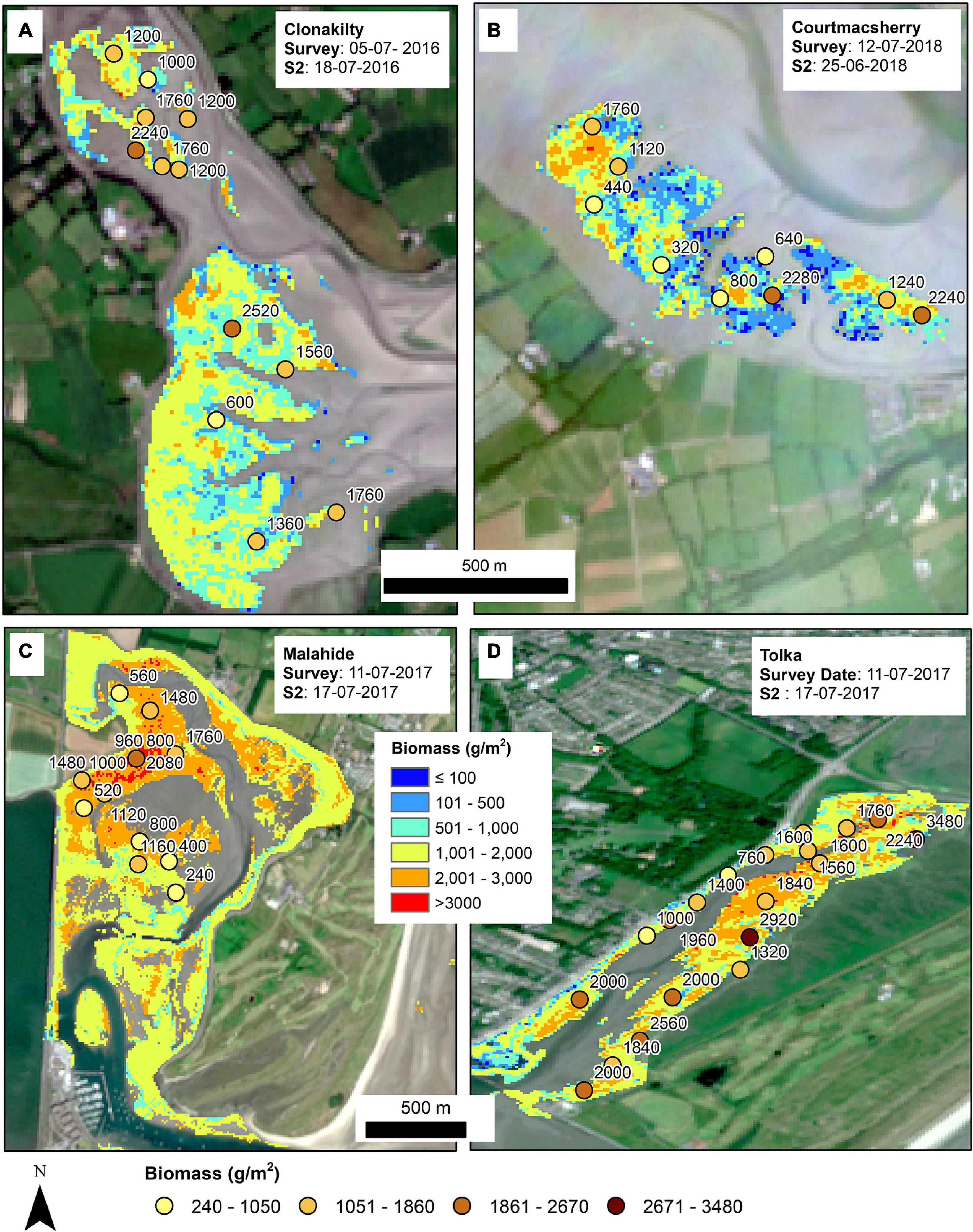
Figure 9. Biomass distribution for four estuaries: (A) Clonakilty, (B) Courtmacsherry, (C) Malahide, and (D) Tolka. The field measured samples from the in situ survey are shown as points. The dates of field survey and Sentinel-2 acquisitions are also shown.

Discussion

Spatial Coverage of the Bloom

The current study used the visible and NIR bands from the optical sensors and used the NDVI delineation technique along the tidal flats. Overall, the NDVI technique showed a fine-scale delineation of blooms than those measured in the field. The reason for a generally better delineation for the EO estimation could be due to its sensitivity to even small algal patches including microphytobenthos present in the sediment (Launeau et al., 2018). It seems more evident on Sentinel-2 than Landsat, most likely because of its higher spatial resolution. In contrast, the field survey is generally restricted to the main areas of the intertidal environment that can be accessed, as shown in Figure 4. Considering the increasing average monthly rainfall in Ireland (80–130 mm; Walsh, 2012) and associated cloud coverage, it is difficult to limit the temporal gaps to a couple of days or exclusively select scenes either before or after the field surveys. Despite this, a good correlation was obtained followed by a negligible bias and a slope close to one between satellite estimates and field survey results, as during the peak bloom phase (from June to September), the bloom extension might remain more or less constant (relative standard deviation 13–18%; Monagail et al., 2021, unpublished data).

Despite these satisfactory results, there may be small variations in the estimates due to the growth of the bloom during the time between the satellite overpass and the field surveys. This may explain relatively lower Cohen’s Kappa in few locations (around 0.4, Figure 7). Similarly, the movement of the large quantities of seaweed biomass because of wind and tidal currents (Gower et al., 2008; Qiao et al., 2009; Cui et al., 2012) has not been considered in this study because algal mats producing blooms in Irish estuaries are mostly attached to the substrate. Additionally, variation in NDVI can arise from the different stages of macroalgal blooms such as healthy and photosynthetically active versus decomposing macroalgal tissue that can give rise to slightly different measures of NDVI leading to small variations in the spatial coverage. The NDVI-based technique eliminates the need to filter out dead or decomposed vegetation mapped in contrast to other indices that rely entirely on the spectral reflectance on the visible part of the spectrum such as red, green, or blue regions. Due to the seasonal growth of the macroalgae, the rate of photosynthesis varies with time, thus the use of NDVI can correctly account for the corresponding variation in electromagnetic signals indicative of vegetation health (Erener, 2011; Turvey and Mclaurin, 2012). This is particularly important in our case because macroalgal blooms may consist of algae at various states of life cycle such as mature algal tissue or actively decomposing mass. Furthermore, minor discrepancies may have resulted from the methodologies currently being adopted during the field measurements including human error and sampling bias. These issues were unavoidable considering environmental constraints such as high-cloud coverage, high-tide conditions, and field limitations such as field safety and accessibility. Planning of the field surveys around the satellite overpass can help avoid inconsistencies due to daily changes in coverages (Carl et al., 2014). Additionally, there could be some unavoidable errors in the estimation due to the signal mixing that occurs when blooms are present along a pixel boundary. Regardless of the sources of error, our data showed an excellent fit when assessing bloom coverage with very high R² (0.94) value with average Kappa value of 0.69 ± 0.13 suggesting a good agreement between field and EO observation.

The above observations provide evidence that the mapping results from 10 and 30 m resolutions did not differ significantly at the current scale of monitoring of algal blooms. This finding is especially helpful in an Irish context, where the number of scenes is particularly limited by the cloud cover as well as low-tide conditions. For areas with optimal weather conditions, it offers the additional advantage of more frequent monitoring. Taking into account the average monthly rainfall of 80 mm even during the drier months (April–July) and 130 mm during the wetter months (October–January) (Walsh, 2012) in Ireland, it is important to note that rainfall and cloud conditions are relatively higher here than in many other countries. Amid these limitations, in the situation where appropriate Sentinel-2 scenes are not available, Landsat acquisitions could still be used for mapping the blooms in these estuaries without greatly compromising the quality of the results. In addition, data from the legacy Landsat acquisitions or any other optical missions could be utilized to reconstruct and analyze the trend of historical blooms in any area (e.g., Bermejo et al., 2020).

The results from the current study show the higher overall effectiveness of the NDVI technique compared to similar findings elsewhere (Cavanaugh et al., 2010; Siddiqui and Zaidi, 2016; Siddiqui et al., 2019; Taddia et al., 2019). Intertidal green algae and giant kelp were mapped using the Sentinel-2 imagery, where only 66% of field survey locations showed the presence of kelp within a distance of 300 m (Mora-Soto et al., 2020). A similar study (Fauzan et al., 2017) conducted using Sentinel-2 for acquiring the percentage coverage of seagrass showed an overall accuracy of 61% with a coefficient of determination of 0.51. Occasionally, the adopted technology was only limited to the size of the study area (area > 10,000 m²; Mora-Soto et al., 2020), whereas the current study could map the bloom to the minimum extent of a few pixels using the NDVI delineation technique. The greater effectiveness in the present study can be explained by the combination of the adopted AOI delineation technique and the greatly reduced biodiversity of eutrophic mudflats which are mostly covered with Ulva alone. This approach may be challenging to implement in other more biodiverse intertidal areas.

Biomass Computation of the Algal Blooms

The biomass showed a high level of correlation with the red reflectance of the Ulva bloom (Figure 8C). This is expected because of the increased reflectance of the plants in the visible and NIR region (Jensen, 1986). Reflectance in the green region of the electromagnetic spectrum also shows good correlation with the algal biomass, like any green vegetation. The radar indicates low levels of correlation, but the inclusion of the backscatter slightly improved the model performance, probably because of the non-linear contribution of radar that is considered in ANN. The correlation with red reflectance was negative, whereas it was positive with the rest of the variables. Inclusion of NDVI, which is a quantitative measure of healthy vegetation, ensured that only live and photosynthetically active algal tissue was considered. This is the reason why the biomass model was applied only in the area primarily delineated by the NDVI technique.

The biomass predicted using the input variables was compared with the biomass data collected from the field survey (Figure 8E). There seems to be a higher level of correspondence between the modeled and true value as exhibited by the R² value (0.74) and the low RMSE (471.70) considering the relatively small number of training samples (number size: 346). Movement of bloom patches due to tides, wind, positional error due to GPS, or the growth of blooms during the time period between field surveys and satellite acquisitions might be responsible for outliers in the scatterplot which are not explained by the independent variables (i.e., 26% unexplained by R²). With a greater number of iterations and the addition of hidden layers, the R² value could be increased further, but that could lead to model overfitting, thereby reducing model predictability (Zhang et al., 1998; Jin et al., 2004; Liu et al., 2008). Thus, to preserve the model generalization, the model was trained optimally with the help of error statistics reported during the ANN development. The model training was stopped when the model convergence was reached where the error was minimum for both training and validation.

The distribution pattern of the biomass corresponds with the point data collected during the field surveys. The range of the observed and computed biomass also matches for all the sites. Figure 9 shows the computed biomass for Clonakilty (2016), Courtmacsherry (2018), Malahide (2017), and Tolka (2017). The higher magnitude of biomass seems to be scattered uniformly over the areas where point samples were collected in Clonakilty. In contrast, higher biomass is concentrated mostly in the areas where most of the point samples were taken in case of Malahide which shows some level of sampling bias in the adopted methodology. The biomass distribution in both Courtmacsherry and Tolka show the uniform distribution and good correspondence with the field survey data points as shown in Figure 9. Although the results from the ANN are not optimal, the model can be significantly improved with the inclusion of more training samples. With the addition of more samples, the robust point-to-point data calibration and validation exercise could be accomplished in the field considering the biomass estimation at 10 m resolution.

Conclusion

This work involves the validation of EO data-processing techniques to develop a methodology for mapping spatial distribution and biomass of estuarine and coastal macroalgal blooms that can be easily implemented. The predicted results were compared with previously collected historical field survey data for ground-truthing the model outputs. The application of EO data sets from Sentinel-2, Landsat-5, and Landsat-8 was investigated to map seaweed blooms at eight different estuarine locations covering moderate, poor, and bad ecological status as designated by the WFD monitoring program. The study combined EO imagery and field survey data from 2010 to 2018 to map green algae, mostly Ulva blooms. The percentage coverage was computed and compared with the results from the ground, where EO estimates showed a good correlation with the corresponding field results which is very satisfactory for WFD monitoring. Both Sentinel-2 and Landsat imagery provided better estimates despite their different spatial resolutions. The findings show that the resampled Sentinel-2 bands still provide results close to the ones from the original bands.

An ANN model was developed using several determining variables to compute the biomass in the areas already delineated by the NDVI mapping technique. The results of the biomass computed using the ANN show excellent correspondence with the general distribution of the biomass survey results. The model presents significant potential for improvement with the addition of more data points. The current work presents the exploratory efforts to investigate the use of machine learning and artificial intelligence for remote sensing. The ANN model showed the R² value of 0.74 with an RMSE of 471.70. Therefore, this study demonstrates that with the combination of remote sensing derived variables, it is possible to delineate as well as quantify the magnitude of the seaweed blooms.

Future work could involve planning of fieldwork intending to study the influence of resolution on the estimation of coverage. The sampling methodology should be improved to reduce sampling bias and sampling coverage should be increased. These improvements will help to account for variance in the biomass currently not explained by the modeling. Preparation of the fieldwork includes scheduling of the fieldwork during the satellite overpass time around cloud-free days to optimize the number of scenes. This will help obtain more accurate estimates by minimizing the temporal gap between scene acquisition and field surveys. Additional biomass samples will be collected to retrain the ANN model so that the error could be minimized, and optimum performance could be achieved. The developed technique is easily replicable, cost-effective, and has the potential to be implemented as an effective monitoring tool because of its low overhead and extensive geographical coverage. The study has demonstrated that both the NDVI-based technique to map spatial coverage of macroalgal blooms and the ANN-based model to compute biomass have the potential to become an effective complementary tool for monitoring macroalgal blooms where the existing monitoring efforts can leverage the benefits of EO data sets.

Data Availability Statement

The original contributions presented in the study are included in the article/supplementary material. Further inquiries can be directed to the corresponding author/s.

Author Contributions

SK processed the remote sensing data and prepared the manuscript. LM secured the funding for the project. LM, RB, and RW supervised the project and helped in the manuscript development. RB, RW, LM, and MM collected the field data. RB helped in statistical analysis. AM supported in computing and technical works. ED, MH, JH, P-EM, and OF helped in interpreting the results. All authors contributed to the article and approved the submitted version.

Funding

The research was funded through the 2014-2020 EPA Research Strategy (EPA, Ireland, Project No: 2018-W-MS-32 “the MACRO-MAN” project).

Conflict of Interest

The authors declare that the research was conducted in the absence of any commercial or financial relationships that could be construed as a potential conflict of interest.

Acknowledgments

The authors would like to thank EPA for providing field survey and historical monitoring data.

Footnotes

1. ^ www.catchments.ie
2. ^ https://earthexplorer.usgs.gov/
3. ^ https://scihub.copernicus.eu/
4. ^ https://www.epa.ie/pubs/data/corinedata/

References

Abadi, M., Barham, P., Chen, J., Chen, Z., Davis, A., Dean, J., et al. (2016). “TensorFlow: a system for large-scale machine learning,” in Proceedings of the 12th USENIX Symposium on Operating Systems Design and Implementation (OSDI), Savannah, GA), 265–283.

Google Scholar

Agatonovic-Kustrin, S., and Beresford, R. (2000). Basic concepts of artificial neural network (ANN) modeling and its application in pharmaceutical research. J. Pharm. Biomed. Anal. 22, 717–727. doi: 10.1016/S0731-7085(99)00272-1

CrossRef Full Text | Google Scholar

Aggarwal, C. C. (2018). Neural networks and deep learning. Springer 10, 978–983.

Google Scholar

Airoldi, L., and Beck, M. W. (2007). Loss, status and trends for coastal marine habitats of Europe. Oceanogr. Mar. Biol. Ann. Rev. 45, 345–405.

Google Scholar

Ali, I., Greifeneder, F., Stamenkovic, J., Neumann, M., and Notarnicola, C. (2015). Review of machine learning approaches for biomass and soil moisture retrievals from remote sensing data. Remote Sens. 7, 16398–16421. doi: 10.3390/rs71215841

CrossRef Full Text | Google Scholar

Alwosheel, A., van Cranenburgh, S., and Chorus, C. G. (2018). Is your dataset big enough? Sample size requirements when using artificial neural networks for discrete choice analysis. J. Choice Model. 28, 167–182. doi: 10.1016/j.jocm.2018.07.002

CrossRef Full Text | Google Scholar

Apitz, S. E., Elliott, M., Fountain, M., and Galloway, T. S. (2006). European environmental management: moving to an ecosystem approach. Integr. Environ. Assess. Manag. 2, 80–85. doi: 10.1002/ieam.5630020114

CrossRef Full Text | Google Scholar

Bannari, A., Morin, D., Bonn, F., and Huete, A. R. (2009). A review of vegetation indices. Remote Sens. Rev. 13, 95–120. doi: 10.1080/02757259509532298

CrossRef Full Text | Google Scholar

Bardenet, R., Brendel, M., Kégl, B., and Sebag, M. (2013). “Collaborative hyperparameter tuning,” in Proceedings of the 30th International Conference on Machine Learning, PMLR, Friedrichshafen, 199–207.

Google Scholar

Bell, T. W., Cavanaugh, K. C., and Siegel, D. A. (2015). Remote monitoring of giant kelp biomass and physiological condition: an evaluation of the potential for the Hyperspectral Infrared Imager (HyspIRI) mission. Remote Sens. Environ. 167, 218–228. doi: 10.1016/j.rse.2015.05.003

CrossRef Full Text | Google Scholar

Bermejo, R., de la Fuente, G., Vergara, J. J., and Hernández, I. (2013). Application of the CARLIT index along a biogeographical gradient in the Alboran Sea (European Coast). Mar. Pollut. Bull. 72, 107–118. doi: 10.1016/j.marpolbul.2013.04.011

PubMed Abstract | CrossRef Full Text | Google Scholar

Bermejo, R., Heesch, S., Monagail, M. M., O’Donnell, M., Daly, E., Wilkes, R. J., et al. (2019a). Spatial and temporal variability of biomass and composition of green tides in Ireland. Harmful Algae. 81, 94–105. doi: 10.1016/j.hal.2018.11.015

PubMed Abstract | CrossRef Full Text | Google Scholar

Bermejo, R., Heesch, S., O’Donnell, M., Golden, N., MacMonagail, M., Edwards, M. D., et al. (2019b). Nutrient dynamics and ecophysiology of opportunistic macroalgal blooms in Irish estuaries and coastal bays (Sea-MAT). Environ. Protect. Agency Irel. Res. Rep. 285:156.

Google Scholar

Bermejo, R., Vergara, J. J., and Hernández, I. (2012). Application and reassessment of the reduced species list index for macroalgae to assess the ecological status under the Water Framework Directive in the Atlantic coast of Southern Spain. Ecol. 12, 46–57. doi: 10.1016/j.ecolind.2011.04.008

CrossRef Full Text | Google Scholar

Bermejo, R., MacMonagail, M., Heesch, S., Mendes, A., Edwards, M., Fenton, O., et al. (2020). The arrival of a red invasive seaweed to a nutrient over-enriched estuary increases the spatial extent of macroalgal blooms. Mar. Environ. Res. 158:104944. doi: 10.1016/j.marenvres.2020.104944

PubMed Abstract | CrossRef Full Text | Google Scholar

Boon, P. J., Clarke, S. A., and Copp, G. H. (2020). Alien species and the EU Water framework directive: a comparative assessment of European approaches. Biol. Invasions. 22, 1497–1512. doi: 10.1007/s10530-020-02201-z

CrossRef Full Text | Google Scholar

Borja, A. (2005). The European water framework directive: a challenge for nearshore, coastal and continental shelf research. Cont. Shelf Res. 25, 1768–1783. doi: 10.1016/j.csr.2005.05.004

CrossRef Full Text | Google Scholar

Borja, A., and Elliott, M. (2013). Marine monitoring during an economic crisis: The cure is worse than the disease. Mar. Pollut. Bull. 68, 1–3. doi: 10.1016/j.marpolbul.2013.01.041

PubMed Abstract | CrossRef Full Text | Google Scholar

Bourquin, J., Schmidli, H., van Hoogevest, P., and Leuenberger, H. (1998). Advantages of Artificial Neural Networks (ANNs) as alternative modelling technique for data sets showing non-linear relationships using data from a galenical study on a solid dosage form. Eur. J. Pharm. Sci. 7, 5–16. doi: 10.1016/S0928-0987(97)10028-8

CrossRef Full Text | Google Scholar

Carl, C., de Nys, R., and Paul, N. A. (2014). The seeding and cultivation of a tropical species of filamentous Ulva for algal biomass production. PLoS One. 9:e98700. doi: 10.1371/journal.pone.0098700

PubMed Abstract | CrossRef Full Text | Google Scholar

Carvalho, L., Mackay, E. B., Cardoso, A. C., Baattrup-Pedersen, A., Birk, S., Blackstock, K. L., et al. (2019). Protecting and restoring Europe’s waters: An analysis of the future development needs of the Water Framework Directive. Sci. Total Environ. 658, 1228–1238. doi: 10.1016/j.scitotenv.2018.12.255

PubMed Abstract | CrossRef Full Text | Google Scholar

Casal, G., Sánchez-Carnero, N., Sánchez-Rodríguez, E., and Freire, J. (2011). Remote sensing with SPOT-4 for mapping kelp forests in turbid waters on the south European Atlantic shelf. Estuar. Coast. Shelf Sci. 91, 371–378. doi: 10.1016/j.ecss.2010.10.024

CrossRef Full Text | Google Scholar

Cavanaugh, K. C., Siegel, D. A., Kinlan, B. P., and Reed, D. C. (2010). Scaling giant kelp field measurements to regional scales using satellite observations. Mar. Ecol. Prog. Ser. 403, 13–27. doi: 10.3354/meps08467

CrossRef Full Text | Google Scholar

Cavanaugh, K. C., Siegel, D. A., Reed, D. C., and Dennison, P. E. (2011). Environmental controls of giant-kelp biomass in the Santa Barbara Channel, California. Mar. Ecol. Prog. Ser. 429, 1–17. doi: 10.3354/meps09141

CrossRef Full Text | Google Scholar

Chang, J., and Shoshany, M. (2016). “Mediterranean shrublands biomass estimation using Sentinel-1 and Sentinel-2,” in Proceedings of the 2016 IEEE International Geoscience and Remote Sensing Symposium (IGARSS), Beijing, 5300–5303.

Google Scholar

Cloern, J. E. (2001). Our evolving conceptual model of the coastal eutrophication problem. Mar. Ecol. Prog. Ser. 210, 223–253. doi: 10.3354/meps210223

CrossRef Full Text | Google Scholar

Conser, E., and Shanks, A. L. (2019). Density of benthic macroalgae in the intertidal zone varies with surf zone hydrodynamics. Phycologia. 58, 254–259. doi: 10.1080/00318884.2018.1557917

CrossRef Full Text | Google Scholar

Costanza, R., d’Arge, R., de Groot, R., Farber, S., Grasso, M., Hannon, B., et al. (1997). The value of the world’s ecosystem services and natural capital. Nature 387, 253–260. doi: 10.1038/387253a0

CrossRef Full Text | Google Scholar

Crabbe, R. A., Lamb, D. W., Edwards, C., Andersson, K., and Schneider, D. (2019). A preliminary investigation of the potential of sentinel-1 radar to estimate pasture biomass in a grazed pasture landscape. Remote Sens. 11:872. doi: 10.3390/rs11070872

CrossRef Full Text | Google Scholar

Cristina, S., Icely, J., Goela, P., DelValls, T., and Newton, A. (2015). Using remote sensing as a support to the implementation of the European Marine Strategy Framework Directive in SW Portugal. Cont. Shelf Res. 108, 169–177. doi: 10.1016/j.csr.2015.03.011

CrossRef Full Text | Google Scholar

Cui, T. W., Zhang, J., Sun, L. E., Jia, Y. J., Zhao, W., Wang, Z. L., et al. (2012). Satellite monitoring of massive green macroalgae bloom (GMB): imaging ability comparison of multi-source data and drifting velocity estimation. Int. J. Remote Sens. 33, 5513–5527. doi: 10.1080/01431161.2012.663112

CrossRef Full Text | Google Scholar

Dayhoff, J. E., and DeLeo, J. M. (2001). Artificial neural networks: opening the black box. Cancer 91, 1615–1635.

Google Scholar

Diaz, R. J., and Rosenberg, R. (2008). Spreading dead zones and consequences for marine ecosystems. Science. 321, 926–929. doi: 10.1126/science.1156401

PubMed Abstract | CrossRef Full Text | Google Scholar

D’Odorico, P., Gonsamo, A., Damm, A., and Schaepman, M. E. (2013). Experimental evaluation of Sentinel-2 spectral response functions for NDVI time-series continuity. IEEE Trans. Geosci. Remote Sens. 51, 1336–1348. doi: 10.1109/TGRS.2012.2235447

CrossRef Full Text | Google Scholar

Donkersloot, R., and Menzies, C. (2015). Place-based fishing livelihoods and the global ocean: The Irish pelagic fleet at home and abroad. Marit. Stud. 14, 1–19. doi: 10.1186/s40152-015-0038-5

CrossRef Full Text | Google Scholar

Donnellan, M. D., and Foster, M. S. (1999). Effects of Small-Scale Kelp Harvesting on Giant Kelp Surface Canopy Dynamics in the Ed Ricketts Underwater Park Region, Final Report to the Monterey Bay National Marine Sanctuary and the Cities of Monterey and Pacific Grove. Monterey, CA: Bay National Marine Sanctuary.

Google Scholar

Duffy, J. P., Pratt, L., Anderson, K., Land, P. E., and Shutler, J. D. (2018). Spatial assessment of intertidal seagrass meadows using optical imaging systems and a lightweight drone. Estuar. Coast. Shelf Sci. 200, 169–180. doi: 10.1016/j.ecss.2017.11.001

CrossRef Full Text | Google Scholar

EPA (2006). EU Water Framework Directive Monitoring Programme. EPA. Available online at: http://www.epa.ie/pubs/reports/water/other/wfd/ (accessed December 1, 2019).

Google Scholar

EPA (2019). Water Quality in Ireland 2013-2018. EPA. Available online at: https://www.epa.ie/pubs/reports/water/waterqua/waterqualityinireland2013-2018.html (accessed December 1, 2019).

Google Scholar

Erener, A. (2011). Remote sensing of vegetation health for reclaimed areas of Seyitömer open cast coal mine. Int. J. Coal Geol. 86, 20–26. doi: 10.1016/j.coal.2010.12.009

CrossRef Full Text | Google Scholar

ESA (2019). Sentinel 2 resolution and swath. Available online at: https://sentinel.esa.int/web/sentinel/missions/sentinel-2/instrument-payload/resolution-and-swath (accessed March 10, 2019).

Google Scholar

European Commission (2000). Directive 2000/60/EC of the European Parliament and of the Council of 23 October 2000 establishing a framework for community action in the field of water policy. Off. J. Eur. Commun. 327, 1–72.

Google Scholar

European Commission (2008). Directive2008/56/EC of the European Parliament and of the Council of 17 June 2008, establishing a framework for community action in the field of marine environmental policy (Marine Strategy Framework Directive). Off. J. Eur. Commun. 164, 19–40.

Google Scholar

Eyre, B. D., and Ferguson, A. J. P. (2002). Comparison of carbon production and decomposition, benthic nutrient fluxes and denitrification in seagrass, phytoplankton, benthic microalgal and macroalgal dominated warm temperate Australian lagoons. Mar. Ecol. Prog. Ser. 229, 43–59. doi: 10.3354/meps229043

CrossRef Full Text | Google Scholar

Fauzan, M. A., Kumara, I. S. W., Yogyantoro, R. N., Suwardana, S. W., Fadhilah, N., Nurmalasari, I., et al. (2017). Assessing the capability of sentinel-2A data for mapping seagrass percent cover in Jerowaru. East Lombok. Indones. J. Geogr. 49, 195–203. doi: 10.22146/ijg.28407

CrossRef Full Text | Google Scholar

Filipponi, F. (2019). Sentinel-1 GRD preprocessing workflow. Proceedings 2019:11. doi: 10.3390/ECRS-3-06201

CrossRef Full Text | Google Scholar

Fyfe, J. E., Israel, S. A., Chong, A., Ismail, N., Hurd, C. L., and Probert, K. (1999). Mapping marine habitats in Otago, southern New Zealand. Geocarto Int. 14, 17–28. doi: 10.1080/10106049908542113

CrossRef Full Text | Google Scholar

Garroutte, E. L., Hansen, A. J., and Lawrence, R. L. (2016). Using NDVI and EVI to map spatiotemporal variation in the biomass and quality of forage for migratory elk in the Greater Yellowstone Ecosystem. Remote Sens. 8:404. doi: 10.3390/rs8050404

CrossRef Full Text | Google Scholar

Geng, X., Li, P., Yang, J., Shi, L., Li, X. M., and Zhao, J. (2020). “Ulva prolifera detection with dual-polarization GF-3 SAR data,” in Proceedings of the IOP Conference Series: Earth and Environmental Science, Vol. 502, 012026.

Google Scholar

Gower, J., Hu, C., Borstad, G., and King, S. (2006). Ocean color satellites show extensive lines of floating Sargassum in the Gulf of Mexico. IEEE Trans. Geosci. Remote Sens. 44, 3619–3625. doi: 10.1109/TGRS.2006.882258

CrossRef Full Text | Google Scholar

Gower, J., King, S., and Goncalves, P. (2008). Global monitoring of plankton blooms using MERIS MCI. Int. J. Remote. Sens. 29, 6209–6216. doi: 10.1080/01431160802178110

CrossRef Full Text | Google Scholar

Hame, T., Rauste, Y., Antropov, O., Ahola, H. A., and Kilpi, J. (2013). Improved mapping of tropical forests with optical and SAR imagery, Part II: above ground biomass estimation. IEEE J. Sel. Top. Appl. Earth. Obs. Remote Sens. 6, 92–101. doi: 10.1109/JSTARS.2013.2241020

CrossRef Full Text | Google Scholar

Hering, D., Borja, A., Carstensen, J., Carvalho, L., Carvalho, L., Feld, C. K., et al. (2010). The European water framework directive at the age of 10: a critical review of the achievements with recommendations for the future. Sci. Total Environ. 408, 4007–4019. doi: 10.1016/j.scitotenv.2010.05.031

PubMed Abstract | CrossRef Full Text | Google Scholar

Hernandez-Cruz, L. R., Purkis, S. J., and Riegl, B. M. (2006). Documenting decadal spatial changes in seagrass and Acropora palmata cover by aerial photography analysis in Vieques, Puerto Rico: 1937–2000. Bull. Mar. Sci. 79, 401–414.

Google Scholar

Hu, C., Wu, Q., Li, H., Jian, S., Li, N., and Lou, Z. (2018). Deep learning with a long short-term memory networks approach for rainfall-runoff simulation. Water. 10:1543. doi: 10.3390/w10111543

CrossRef Full Text | Google Scholar

Hu, L., Hu, C., and Ming-Xia, H. E. (2017). Remote estimation of biomass of Ulva prolifera macroalgae in the Yellow Sea. Remote Sens. Environ. 192, 217–227. doi: 10.1016/j.rse.2017.01.037

CrossRef Full Text | Google Scholar

Huang, Y. (2009). Advances in artificial neural networks—Methodological development and application. Algorithms 2, 973–1007. doi: 10.3390/algor2030973

CrossRef Full Text | Google Scholar

Huete, A., Didan, K., Miura, T., Rodriguez, E. P., Gao, X., and Ferreira, L. G. (2002). Overview of the radiometric and biophysical performance of the MODIS vegetation indices. Remote Sens. Environ. 83, 195–213. doi: 10.1016/S0034-4257(02)00096-2

CrossRef Full Text | Google Scholar

Jeffrey, D. W., Brennan, M. T., Jennings, E., Madden, B., and Wilson, J. G. (1995). Nutrient sources for in-shore nuisance macroalgae: The Dublin Bay case. Ophelia 42, 147–161. doi: 10.1080/00785326.1995.10431501

CrossRef Full Text | Google Scholar

Jensen, J. R. (1986). Introductory Digital Image Processing. Upper Saddle River, NJ: Prentice-Hall, 592.

Google Scholar

Jha, C. S., Rangaswamy, M., Murthy, M. S. R., and Vyjayanthi, N. (2006). Estimation of forest biomass using Envisat-ASAR data. Proc. SPIE 6410:641002.

Google Scholar

Jiang, X., Gao, Z., Zhang, Q., Wang, Y., Tian, X., Shang, W., et al. (2020). Remote sensing methods for biomass estimation of green algae attached to nursery-nets and raft rope. Pollut. Bull. 150:110678. doi: 10.1016/j.marpolbul.2019.110678

PubMed Abstract | CrossRef Full Text | Google Scholar

Jin, L., Kuang, X., and Haung, H. (2004). Study on the overfitting of the Artificial Neural Network forecasting model. Acta. Meteorol. Sin. 62, 62–69.

Google Scholar

Karki, S., Sultan, M., Elkadiri, R., and Elbayoumi, T. (2018). Mapping and forecasting onsets of harmful algal blooms using MODIS data over coastal waters surrounding Charlotte County. Florida. Remote Sens. 10:1656. doi: 10.3390/rs10101656

CrossRef Full Text | Google Scholar

Karlaftis, M. G., and Vlahogianni, E. I. (2011). Statistical methods versus neural networks in transportation research: differences, similarities and some insights. Transp. Res. Part C Emerg. Technol. 19, 387–399. doi: 10.1016/j.trc.2010.10.004

CrossRef Full Text | Google Scholar

Ke, Y., Im, J., Lee, J., Gong, H., and Ryu, Y. (2015). Characteristics of Landsat 8 OLI-derived NDVI by comparison with multiple satellite sensors and in-situ observations. Remote Sens. Environ. 164, 298–313. doi: 10.1016/j.rse.2015.04.004

CrossRef Full Text | Google Scholar

Kim, E., Kim, K., Kim, S. M., Cui, T., and Ryu, J. H. (2020). Deep learning based floating macroalgae classification using Gaofen-1 WFV images. Kor. J. Remote Sens. 36, 293–307. doi: 10.7780/kjrs.2020.36.2.2.6

CrossRef Full Text | Google Scholar

Kotta, J., Valdivia, N., Kutser, T., Toming, K., Rätsep, M., and Orav-Kotta, H. (2018). Predicting the cover and richness of intertidal macroalgae in remote areas: a case study in the Antarctic Peninsula. Ecol. Evol. 8, 9086–9094. doi: 10.1002/ece3.4463

PubMed Abstract | CrossRef Full Text | Google Scholar

Kutser, T., Hedley, J., Giardino, C., Roelfsema, C., and Brando, V. E. (2020). Remote sensing of shallow waters–A 50 year retrospective and future directions. Remote Sens. Environ. 240:111619. doi: 10.1016/j.rse.2019.111619

CrossRef Full Text | Google Scholar

Launeau, P., Méléder, V., Verpoorter, C., Barillé, L., Kazemipour-Ricci, F., Giraud, M., et al. (2018). Microphytobenthos biomass and diversity mapping at different spatial scales with a hyperspectral optical model. Remote Sens. 10:16. doi: 10.3390/rs10050716

CrossRef Full Text | Google Scholar

Laurin, G. V., Balling, J., Corona, P., Mattioli, W., Papale, D., Puletti, N., et al. (2018). Above-ground biomass prediction by Sentinel-1 multitemporal data in central Italy with integration of ALOS2 and Sentinel-2 data. J. Appl. Remote Sens. 12:016008. doi: 10.1117/1.JRS.12.016008

CrossRef Full Text | Google Scholar

Le Toan, T., Quegan, S., Davidson, M. W. J., and Baltzer, H. (2011). The BIOMASS mission: mapping global forest biomass to better understand the terrestrial carbon cycle. Remote Sens. Environ. 115, 2850–2860. doi: 10.1016/j.rse.2011.03.020

CrossRef Full Text | Google Scholar

Liang, X. J., Qin, P., Xiao, Y. F., Kim, K. Y., Liu, R. J., Chen, X. Y., et al. (2019). Automatic remote sensing detection of floating macroalgae in the yellow and east china seas using extreme learning machine. J. Coast. Res. 90, 272–281. doi: 10.2112/SI90-034.1

CrossRef Full Text | Google Scholar

Liu, Y., Starzyk, J. A., and Zhu, Z. (2008). Optimized approximation algorithm in neural networks without overfitting. IEEE Trans. Neural. Netw. 19, 983–995. doi: 10.1109/TNN.2007.915114

PubMed Abstract | CrossRef Full Text | Google Scholar

Lotze, H. K., Lenihan, H. S., Bourque, B. J., Bradbury, R. H., Cooke, R. G., Kay, M. C., et al. (2006). Depletion, degradation, and recovery potential of estuaries and coastal seas. Science 312, 1806–1809. doi: 10.1126/science.1128035

PubMed Abstract | CrossRef Full Text | Google Scholar

Mora-Soto, A., Palacios, M., Macaya, E. C., Gómez, I., Huovinen, P., Pérez-Matus, A., et al. (2020). A high-resolution global map of giant kelp (Macrocystis pyrifera) forests and intertidal green algae (Ulvophyceae) with Sentinel-2 imagery. Remote Sens. 12:694. doi: 10.3390/rs12040694

CrossRef Full Text | Google Scholar

Nadikattu, R. R. (2017). The supremacy of artificial intelligence and neural networks. Int. J. Creat. Res. Thoughts 5, 950–954.

Google Scholar

Navarro, J. A., Algeet, N., Fernández-Landa, A., Esteban, J., Rodríguez-Noriega, P., and Guillén-Climent, M. L. (2019). Integration of UAV, sentinel-1, and sentinel-2 data for mangrove plantation aboveground biomass monitoring in Senegal. Remote Sens. 11:77. doi: 10.3390/rs11010077

CrossRef Full Text | Google Scholar

Ndikumana, E., Ho Tong Minh, D., Dang Nguyen, H. T., Baghdadi, N., Courault, D., Hossard, L., et al. (2018). Estimation of rice height and biomass using multitemporal SAR Sentinel-1 for Camargue, Southern France. Remote Sens. 10:1394. doi: 10.3390/rs10091394

CrossRef Full Text | Google Scholar

Nezlin, N. P., Kamer, K., and Stein, E. D. (2007). Application of color infrared aerial photography to assess macroalgal distribution in an eutrophic estuary, upper Newport Bay, California. Estuaries Coast. 30, 855–868. doi: 10.1007/BF02841339

CrossRef Full Text | Google Scholar

Ní Longphuirt, S., Boyle, S. O., Wilkes, R., Dabrowski, T., and Stengel, D. B. (2016). Influence of hydrological regime in determining the response of macroalgal blooms to nutrient loading in two Irish estuaries. Estuaries Coast. 39, 478–494. doi: 10.1007/s12237-015-0009-5

CrossRef Full Text | Google Scholar

Norton, D., Hynes, S., and Boyd, J. (2018). Valuing Ireland’s Coastal, Marine and Estuarine Ecosystem Services, Vol. 80. Washington, DC: Environmental Protection Agency.

Google Scholar

O’Brien, R. M. A. (2007). Caution regarding rules of thumb for Variance Inflation Factors. Qual. Quant. 41, 673–690. doi: 10.1007/s11135-006-9018-6

CrossRef Full Text | Google Scholar

Periasamy, S. (2018). Significance of dual polarimetric synthetic aperture radar in biomass retrieval: an attempt on Sentinel-1. Remote Sens. Environ. 217, 537–549. doi: 10.1016/j.rse.2018.09.003

CrossRef Full Text | Google Scholar

Pfister, C. A., Berry, H. D., and Mumford, T. (2017). The dynamics of kelp forests in the northeast Pacific Ocean and the relationship with environmental drivers. J. Ecol. 17, 1–14. doi: 10.1111/1365-2745.12908

CrossRef Full Text | Google Scholar

Piotrowski, A. P., and Napiorkowski, J. J. (2013). A comparison of methods to avoid overfitting in neural networks training in the case of catchment runoff modelling. J. Hydrol. 476, 97–111. doi: 10.1016/j.jhydrol.2012.10.019

CrossRef Full Text | Google Scholar

Praeger, C., Vucko, M. J., McKinna, L., de Nys, R., and Cole, A. (2020). Estimating the biomass density of macroalgae in land-based cultivation systems using spectral reflectance imagery. Algal Res. 50:102009. doi: 10.1016/j.algal.2020.102009

CrossRef Full Text | Google Scholar

Qiao, F., Dai, D., Simpson, J., and Svendsen, H. (2009). Banded structure of drifting macroalgae. Pollut. Bull. 58, 1792–1795. doi: 10.1016/j.marpolbul.2009.08.006

PubMed Abstract | CrossRef Full Text | Google Scholar

Qiu, Z., Li, Z., Bilal, M., Wang, S., Sun, D., and Chen, Y. (2018). Automatic method to monitor floating macroalgae blooms based on multilayer perceptron: case study of Yellow Sea using GOCI images. Opt. Express. 26, 26810–26829. doi: 10.1364/OE.26.026810

PubMed Abstract | CrossRef Full Text | Google Scholar

Raney, K., Freeman, A., Hawkins, B., and Bamler, R. (1994). “A plea for radar brightness,” in Proceedings of the IGARSS ‘94 – 1994 IEEE International Geoscience and Remote Sensing Symposium, Pasadena, CA, 1090–1092.

Google Scholar

Richards, J. A. (2013). Supervised Classification Techniques: Remote Sensing Digital Image Analysis. Berlin: Springer.

Google Scholar

Rossi, F., Incera, M., Callier, M., and Olabarria, C. (2011). Effects of detrital non-native and native macroalgae on the nitrogen and carbon cycling in intertidal sediments. Mar. Biol. 158, 2705–2715. doi: 10.1007/s00227-011-1768-6

CrossRef Full Text | Google Scholar

Rumelhart, D. E., Hinton, G. E., and Williams, R. J. (1986). Learning representations by back-propagating errors. Nature 323, 533–536. doi: 10.1038/323533a0

CrossRef Full Text | Google Scholar

Salarux, C., and Kaewplang, S. (2020). Estimation of algal bloom biomass using UAV-based remote sensing with NDVI and GRVI. Mahasar. Int. J. Eng. Technol. 6, 1–6.

Google Scholar

Scanlan, C. M., Foden, J., Wells, E., and Best, M. A. (2007). The monitoring of opportunistic macroalgal blooms for the water framework directive. Mar. Pollut. Bull. 55, 162–171. doi: 10.1016/j.marpolbul.2006.09.017

PubMed Abstract | CrossRef Full Text | Google Scholar

Schroeder, S. B., Dupont, C., Boyer, L., Juanes, F., and Costa, M. (2019). Passive remote sensing technology for mapping bull kelp (Nereocystis luetkeana): a review of techniques and regional case study. Glob. Ecol. Conserv. 19:e00683. doi: 10.1016/j.gecco.2019.e00683

CrossRef Full Text | Google Scholar

Sfriso, A., Pavoni, B., Marcomini, A., and Orio, A. A. (1992). Macroalgae, nutrient cycles, and pollutants in the lagoon of Venice. Estuaries 14, 517–528. doi: 10.2307/1352394

CrossRef Full Text | Google Scholar

Shahin, M. A., Maier, H. R., and Jaksa, M. B. (2005). “Investigation into the robustness of artificial neural networks for a case study in civil engineering,” in Proeccedings of the MODSIM 2005 International Congress on Modelling and Simulation. Modelling and Simulation Society of Australia and New Zealand, Melbourne, 79–83.

Google Scholar

Siddiqui, M. D., Zaidi, A. Z., and Abdullah, M. (2019). Performance evaluation of newly proposed Seaweed Enhancing Index (SEI). Remote Sens. 11:1434. doi: 10.3390/rs11121434

CrossRef Full Text | Google Scholar

Siddiqui, M., and Zaidi, A. Z. (2016). Worldview-2 and landsat 8 satellite data for seaweed mapping along karachi coast. Pakist. J. Eng. Technol. Sci. 5:920. doi: 10.22555/pjets.v5i2.920

CrossRef Full Text | Google Scholar

Silleos, N. G., Alexandridis, T. K., Gitas, I. Z., and Perakis, K. (2006). Vegetation indices: advances made in biomass estimation and vegetation monitoring in the last 30 years. Geocarto Int. 21, 21–28.

Google Scholar

Small, D. (2011). Flattening gamma: radiometric terrain correction for SAR imagery. IEEE Trans. Geosci. Remote Sens. 49, 3081–3093. doi: 10.1109/TGRS.2011.2120616

CrossRef Full Text | Google Scholar

Small, D., and Schubert, A. (2008). Guide to ASAR Geocoding, RSL. Paris: European Space Agency (ESA).

Google Scholar

Smetacek, V., and Zingone, A. (2013). Green and golden seaweed tides on the rise. Nature 504, 84–88. doi: 10.1038/nature12860

PubMed Abstract | CrossRef Full Text | Google Scholar

Taddia, Y., Russo, P., Lovo, S., and Pellegrinelli, A. (2019). Multispectral UAV monitoring of submerged seaweed in shallow water. Appl. Geomat. 12, 19–34. doi: 10.1007/s12518-019-00270-x

CrossRef Full Text | Google Scholar

Teichberg, M., Fox, S. E., Olsen, Y. S., Valiela, I., Martinetto, P., Iribarne, O., et al. (2010). Eutrophication and macroalgal blooms in temperate and tropical coastal waters: nutrient enrichment experiments with Ulva spp. Glob. Chang. Biol. 16, 2624–2637. doi: 10.1111/j.1365-2486.2009.02108.x

CrossRef Full Text | Google Scholar

Tucker, C., and Sellers, P. (1986). Satellite remote sensing of primary production. Int. J. Remote Sens. 7, 1395–1416. doi: 10.1080/01431168608948944

CrossRef Full Text | Google Scholar

Turvey, C. G., and Mclaurin, M. K. (2012). Applicability of the normalized difference vegetation index (NDVI) in index-based crop insurance design. Weather Clim. Soc. 4, 271–284. doi: 10.1175/WCAS-D-11-00059.1

CrossRef Full Text | Google Scholar

USGS (2020). A Landsat Timeline. Available online at: https://landsat.gsfc.nasa.gov/a-landsat-timeline/ (accessed January 20, 2019).

Google Scholar

Valiela, I., McClelland, J., Hauxwell, J., Behr, P. J., Hersh, D., and Foreman, K. (1997). Macroalgal blooms in shallow estuaries: controls and ecophysiological and ecosystem consequences. Limnol. Oceanogr. 42, 1105–1118. doi: 10.4319/lo.1997.42.5_part_2.1105

PubMed Abstract | CrossRef Full Text | Google Scholar

Veci, L. (2019). SAR basics tutorial, Sentinel-1 Toolbox. European Space Agency. Available online at: http://step.esa.int/docs/tutorials/S1TBX SAR Basics Tutorial.pdf (accessed August 10, 2019).

Google Scholar

Volent, Z., Johnsen, G., and Sigernes, F. (2007). Kelp forest mapping by use of airborne hyperspectral imager. J. Appl. Remote Sens. 1:011503. doi: 10.1117/1.2822611

CrossRef Full Text | Google Scholar

Walsh, S. (2012). A Summary of Climate Averages for Ireland, 1981-2010, Report, Met Éireann, 14, Climatological Note, 2012-05. Glasnevin Hill: Met Éireann.

Google Scholar

Wells, E., Wilkinson, M., Wood, P., and Scanlan, C. (2007). The use of macroalgal species richness and composition on intertidal rocky seashores in the assessment of ecological quality under the European Water Framework Directive. Mar. Pollut. Bull. 55, 151–161. doi: 10.1016/j.marpolbul.2006.08.031

PubMed Abstract | CrossRef Full Text | Google Scholar

Wan, A. H. L., Wilkes, R. J., Heesch, S., Bermejo, R., Johnson, M. P., and Morrison, L. (2017). Assessment and characterisation of Ireland’s green tides (Ulva species). PLoS One 12:e0169049. doi: 10.1371/journal.pone.0169049

PubMed Abstract | CrossRef Full Text | Google Scholar

Wang, J., Xiao, X., Bajgain, R., Starks, P., Steiner, J., Doughty, R. B., et al. (2019). Estimating leaf area index and aboveground biomass of grazing pastures using Sentinel-1, Sentinel-2 and Landsat images. ISPRS J. Photogramm. Remote Sens. 154, 189–201. doi: 10.1016/j.isprsjprs.2019.06.007

CrossRef Full Text | Google Scholar

Wilkes, R., Bennion, M., McQuaid, N., Beer, C., McCullough-Annett, G., Colhoun, K., et al. (2017). Intertidal seagrass in Ireland: pressures, WFD status and an assessment of trace element contamination in intertidal habitats using Zostera noltei. Ecol. Indic. 82, 117–130. doi: 10.1016/j.ecolind.2017.06.036

CrossRef Full Text | Google Scholar

Wilkes, R., Best, M. A., Scanlan, C. M., Rossi, N., Kolbe, K., and Herrero, S. (2018). Coastal and Transitional Waters North East Atlantic Geographic Intercalibration Group: Opportunistic Macroalgae Ecological Assessment Methods. EUR 29594, Publications Office of the European Union, Luxembourg, ISBN 978-92-79-98481-5, JRC115074. Denmark: European Union. doi: 10.2760/167718

CrossRef Full Text | Google Scholar

Xiao, Y. F., Zhang, J., and Cui, T. (2017). High-precision extraction of nearshore green tides using satellite remote sensing data of the Yellow Sea, China. Int. J. Remote Sens. 38, 1626–1641. doi: 10.1080/01431161.2017.1286056

CrossRef Full Text | Google Scholar

Xiao, Y., Zhang, J., Cui, T., Gong, J., Liu, R., Chen, X., et al. (2019). Remote sensing estimation of the biomass of floating Ulva prolifera and analysis of the main factors driving the interannual variability of the biomass in the Yellow Sea. Mar. Pollut. Bull. 140, 330–340. doi: 10.1016/j.marpolbul.2019.01.037

PubMed Abstract | CrossRef Full Text | Google Scholar

Xing, Q., and Hu, C. (2016). Mapping macroalgal blooms in the Yellow Sea and East China Sea using HJ-1 and Landsat data: application of a virtual baseline reflectance height technique. Remote Sens. Environ. 178, 113–126. doi: 10.1016/j.rse.2016.02.065

CrossRef Full Text | Google Scholar

Xu, F., Gao, Z., Jiang, X., Ning, J., Zheng, X., Song, D., et al. (2017). Mapping of green tide using true color aerial photographs taken from a unmanned aerial vehicle. Rem. Sens. Model. Ecosyst. Sustainabil. XIV:104050M. doi: 10.1117/12.2271724

CrossRef Full Text | Google Scholar

Xu, M., Fralick, D., Zheng, J. Z., Wang, B., Tu, X. M., and Feng, C. (2017). The differences and similarities between Two-sample T-Test and Paired T-Test. Shangh. Arch Psychiatry 29, 184–188.

Google Scholar

Xue, J., and Su, B. (2017). Significant remote sensing vegetation indices: A review of developments and applications. J. Sens. 2017:1353691. doi: 10.1155/2017/1353691

CrossRef Full Text | Google Scholar

Zavalas, R., Ierodiaconou, D., Ryan, D., Rattray, A., and Monk, J. (2014). Habitat classification of temperate marine macroalgal communities using bathymetric LiDAR. Remote Sens. 6, 2154–2175. doi: 10.3390/rs6032154

CrossRef Full Text | Google Scholar

Zhang, G., Patuwo, B. E., and Hu, M. Y. (1998). Forecasting with artificial neural networks: the state of the art. Int. J. Forecast. 14, 35–62. doi: 10.1016/S0169-2070(97)00044-7

CrossRef Full Text | Google Scholar

Zhang, H. K., Roy, D. P., Yan, L., Li, Z., Huang, H., Vermote, E., et al. (2018). Characterization of Sentinel-2A and Landsat-8 top of atmosphere, surface, and nadir BRDF adjusted reflectance and NDVI differences. Remote Sens. Environ. 215, 482–494. doi: 10.1016/j.rse.2018.04.031

CrossRef Full Text | Google Scholar

Zhang, J., Shi, J., Gao, S., Huo, Y., Cui, J., Shen, H., et al. (2019). Annual patterns of macroalgal blooms in the Yellow Sea during 2007–2017. PLoS One 14:e0210460. doi: 10.1371/journal.pone.0210460

PubMed Abstract | CrossRef Full Text | Google Scholar

Zhang, Z., Beck, M. W., Winkler, D. A., Huang, B., Sibanda, W., and Goyal, H. (2018). Opening the black box of neural networks: methods for interpreting neural network models in clinical applications. Ann. Transl. Med. 6:216. doi: 10.21037/atm.2018.05.32

PubMed Abstract | CrossRef Full Text | Google Scholar

Zhu, X., and Liu, D. (2015). Improving forest aboveground biomass estimation using seasonal Landsat NDVI time-series. ISPRS J. Photogramm. Remote Sens. 102, 222–231. doi: 10.1016/j.isprsjprs.2014.08.014

CrossRef Full Text | Google Scholar

Zhu, Z., Wulder, M. A., Roy, D. P., Woodcock, C. E., Hansene, M. C., Radeloff, V. C., et al. (2019). Benefits of the free and open Landsat data policy. Remote Sens. Environ. 224, 382–385. doi: 10.1016/j.rse.2019.02.016

CrossRef Full Text | Google Scholar

Zurada, J. M. (1992). Introduction to Artificial Neural System. Boston MA: PWS Publishing.

Google Scholar