Evaluating Uncertainties in Reconstructing the Pre-eutrophic State of the North Sea

Introduction

Eutrophication, i.e., the increase in the supply rate of organic matter (Nixon, 1995), and the inter-linked consequences associated with it, such as hypoxia (Fennel and Testa, 2019), harmful algal blooms (Anderson et al., 2012), and loss of diversity and ecological resilience (Elliott and Whitfield, 2011), are a major concern in coastal systems across the globe, including, but not limited to, the Baltic Sea (e.g., Gustafsson et al., 2012), Black Sea (e.g., Capet et al., 2016), Chesapeake Bay (e.g., Harding et al., 2016), Gulf of Mexico (e.g., Fennel and Laurent, 2018), northern Adriatic Sea (Giani et al., 2012), and Yellow Sea (e.g., Xiao et al., 2017). A recent inter-regional assessment of eutrophication in European seas is presented by Friedland et al. (2021).

In all the above-mentioned examples, eutrophication processes have been “cultural” (Smith, 1998) by means of increased nutrient loading from riverine and atmospheric sources, driven mainly by anthropogenic activities such as intensified farming and industrial activities, as well as dense human populations, resulting in excessive primary production rates in response (Smith, 2006). Such “cause-effect relationship” is also central to the definition of eutrophication by the Oslo-Paris Commission (OSPAR; for an overview to abbreviations see Table 1) as “the enrichment of water by nutrients causing an accelerated growth of algae and higher forms of plant life to produce an undesirable disturbance to the balance of organisms present in the water and to the quality of the water concerned.” It refers to the undesirable effects resulting from anthropogenic enrichment by nutrients (OSPAR, 2017).

TABLE 1

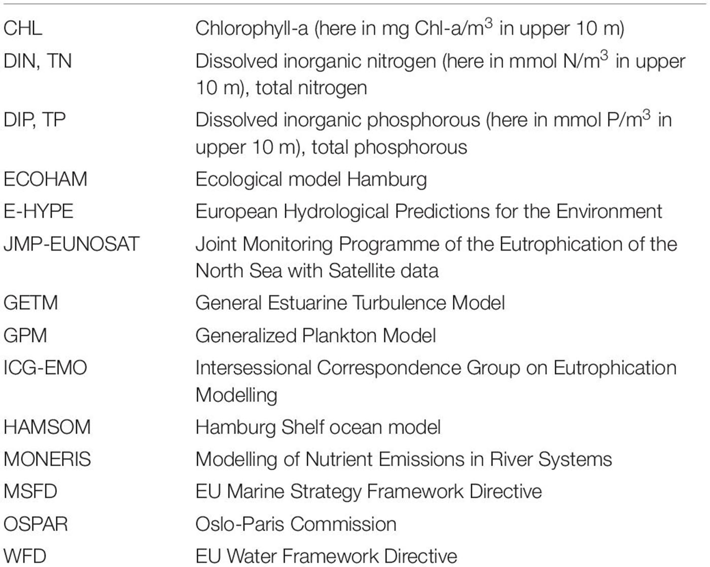
Table 1. List of abbreviations and acronyms.

Natural factors, such as hydrodynamical processes, can modulate the eutrophication response (Cloern, 2001). For instance, in systems characterized by long water residence times or persistent salinity stratification, such as the Baltic Sea and Black Sea, sensitivity to nutrient loading tends to be stronger and meteorological variability or climatic trends can become highly relevant (Oguz et al., 2006; Carstensen et al., 2014). In systems characterized by weak stratification and high turbidity, the primary production response can become dampened, such as in San Francisco Bay (e.g., Cloern and Jassby, 2012). The fact that eutrophication responses are determined by the combination of physical and biogeochemical processes highlights the inter-disciplinary nature of the problem, and the necessity to utilize coupled physical-biogeochemical models.

The North Sea is a semi-enclosed shelf sea adjacent to the northeast Atlantic Ocean. Its circulation is characterized by an anti-cyclonic pattern, driven by a southward Atlantic inflow in the northern North Sea, of which about 85% is recirculated north of the Dogger Bank (Lenhart and Pohlmann, 1997; Pätsch et al., 2017). The circulation south of the Dogger Bank is governed by the English Channel inflow, which follows the continental coast and finally joins the Baltic outflow to leave the North Sea at its north-eastern boundary along the Norwegian Trench. The catchment area covers heavily industrialized and populated regions, that have led to increased eutrophication mainly within the Southern North Sea (SNS) (Emeis et al., 2015), despite the relatively high flushing rates driven by this very dynamic circulation system. Eutrophication problems have been reported for the south-eastern North Sea since the early 1970s (Jickells, 1998). Within the coastal region, increased residence times (Schwichtenberg et al., 2017) and an estuarine-like circulation that leads to trapping of organic matter (Hofmeister et al., 2017) result in an exacerbation of these problems, depending on the distance to riverine inputs and bathymetric features (van Beusekom et al., 2019).

In 1987, OSPAR agreed on a commitment to aim to achieve a substantial reduction (in the order of 50%) of nutrients into regions where these inputs are likely to cause pollution. The ambitious target set for phosphorus has been met, while the reduction target for nitrogen has not yet been achieved by all OSPAR Contracting Parties bordering the North Sea because of the particular difficulties of achieving reductions in nutrients from agricultural sources (Claussen et al., 2009). This led to an increased N:P ratio of the nutrient loads of the major rivers entering the North Sea, likely influencing phytoplankton communities (Brauer et al., 2012) and being less effective in diminishing the risk of harmful algal blooms (Burson et al., 2016). To gain estimates and a realistic timeframe for limiting eutrophication, OSPAR established the Intersessional Correspondence Group on Eutrophication Modelling (ICG-EMO). In a first model comparison, the OSPAR objective to provide nutrient reduction targets that result in more balanced N:P ratios was analyzed (Lenhart et al., 2010). It was the first time that model-based nutrient reduction scenarios have been used in an OSPAR eutrophication assessment. In the meantime, the EU put two legal frameworks into practice: the Water Framework Directive (WFD; European Commission, 2000, 2009) and the Marine Strategy Framework Directive (MSFD; European Commission, 2008). While the WFD mainly focuses on transitional and near-coastal waters, the MSFD covers the European marine waters, like the North Sea and adjacent seas. The aim of the MSFD under Descriptor 5 Eutrophication is to achieve (or restore) the “Good Environmental Status” (GES) in the marine environment (OSPAR, 2003, 2017).

Gathering the OSPAR assessment reports (OSPAR, 2003, 2017), which are based on national assessment reports under the so-called Common Procedure, the EU Commission critically remarked the use of national threshold levels for the eutrophication indicators and demanded a harmonized assessment. In response, OSPAR referred to a model study within the JMP-EUNOSAT project (Enserink et al., 2019; EUNOSAT report). They defined internationally coherent assessment levels and assessment areas that reflect natural conditions independent of national boundaries. To derive ecological relevant threshold values for the assessment areas, it is necessary to determine the reference status of the North Sea not impacted by human-induced pressures (European Commission, 2003; Borja et al., 2012). However, such unaffected regions are not available anymore in the North Sea. Therefore, hindcasts of so-called “historic” conditions that represent the “pre-eutrophic” state of the system need to be considered as background level (European Commission, 2003).

Thereby, two main problems have to be addressed: Firstly, “historic” does not define a specific year. Thus, it was interpreted by the OSPAR forum, in which the historic scenario was defined in view of the MSFD application, that a period with little influence of anthropogenic activities should be selected. This implies a situation before the intensification of industrialization and agricultural production by the use of inorganic nitrogen fertilizer based on the Haber–Bosch process, which corresponds roughly to the end of the 19th century. Secondly, hardly any measurements are available for this period, but just anecdotal evidence that, for example, the water transparency and the macrophyte coverage in the German Bight was still high. In the absence of historical data with sufficient coverage, modeling becomes a viable tool for estimating the reference conditions of a system (European Commission, 2003). To allow the marine models to estimate the reference state (e.g., Schernewski et al., 2015), they need reliable information about the historic nutrient inputs, which were also not observed. Hence, catchment models are applied, e.g., the fine scale model MONERIS was used by Kerimoglu et al (2018), which covers German and Dutch nutrient inputs. The JMP-EUNOSAT project (Enserink et al., 2019; EUNOSAT report) utilized estimates from the Swedish E-HYPE model, which covers the whole North Sea catchment including adjacent sea regions (Blauw et al., 2019).

Since the nutrient inputs from two catchment models, MONERIS and E-HYPE, differ strongly in the complexity of their process formulation, which for example, explains a higher need for more detailed input data for MONERIS that leads to a lower coverage of catchment areas, their impacts on marine environmental conditions are considered separately in the presented study. This is necessary to assess the uncertainty of the simulated historic concentrations of DIN, DIP, and chlorophyll-a, which form the basis for the derivation of the GES target concentration under MSFD. Therefore, investigating the variability in the reaction of the eutrophication indicators under different historic conditions will help to identify problems in the derivation of the threshold values and in the use of the newly defined assessment areas.

In this study, we analyze how different assumptions, like nutrient influx and plankton dynamics, influence the historical status in the North Sea. We further estimate how the resulting differences in the historic simulation can be judged based on comparisons against the differences between the results produced by two different biogeochemical models, and through natural sources of uncertainty. Here, uncertainty is accounted for by spatial, seasonal, and inter-annual variability as resolved by the applied models. Specifically, we determine how uncertainty ranges in model estimates for historic reference conditions compare to ranges of natural variability of nutrient and phytoplankton concentrations.

Materials and Methods

The Model System

For the analysis, we used a nested model system consisting of two ecosystem models. ECOHAM (ECOlogical model HAMburg) has already been used in early stages of the OSPAR modeling activities (OSPAR ICG-EMO; Lenhart et al., 2010). The application for the Northwest European continental shelf (NECS setup) includes the relevant nutrient cycles (nitrogen, phosphorous, and silicate), as well as two state variables for phytoplankton, detritus and zooplankton, bacteria, and oxygen (Lorkowski et al., 2012). ECOHAM uses the same regular 20 km grid as the HAMSOM model, which provides the hydrodynamical forcing files (Figure 1 left). Große et al. (2017) provide an extensive description of this setup and further details of the ECOHAM biogeochemical model. With the NECS-setup ECOHAM covers all national river contributions that are affected by the two scenarios.

FIGURE 1

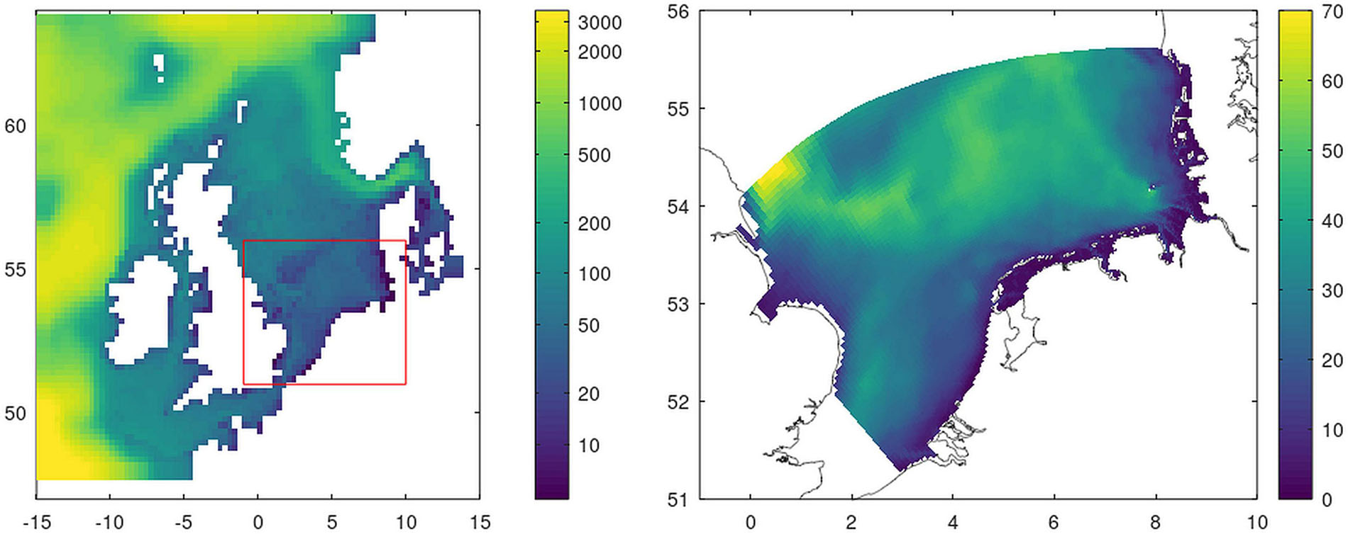
Figure 1. Model systems with model bathymetry. Left: ECOHAM (the red box indicates the region on the right) and Right: GPM.

For a better representation of the steep gradients both in the hydrodynamic (e.g., salinity) as well as for the biogeochemical (e.g., nutrients) conditions in the nearshore regions, we use a second model, which offers a fine-scale grid for the SNS and German Bight. This SNS setup includes GETM as hydrodynamical component (Burchard and Bolding, 2002) to which the newly established biogeochemical “Generalized Plankton Model,” GPM (Kerimoglu et al., 2020) is coupled. GPM consists of a flexible generic plankton module and an ECOHAM-based geochemical component. The setup is established on an irregular grid with a horizontal grid cell resolution of 1.5 km in the coastal region and up to 4.5 km toward the outer boundary (Figure 1 right; Kerimoglu et al., 2017). Along the open ocean boundaries, we used clamp boundary conditions for temperature, salinity, oxygen and all variables bound to DIM, DOM and detritus pools (see Kerimoglu et al., 2020) from ECOHAM, whereas we assume zero-gradient boundary conditions for the variables bound to phytoplankton and zooplankton variables. Therefore, this nested setup is capable of taking into account changes in the river loads outside the SNS-domain and consider them in the representation of GPM.

Forcing Data

Nutrient inputs are based on a riverine database developed within ICG-EMO by Sonja van Leeuwen (NIOZ) covering about 250 rivers within the Northwest European Shelf domain. As part of this database, the river information for the German and Dutch rivers including the Scheldt are provided by the University of Hamburg and described in a technical report (Pätsch and Lenhart, 2019). For the representation of the atmospheric nitrogen deposition, we used data from EMEP¹ (Iversen et al., 1989; Bartnicki et al., 2011) for the relevant years for both models.

Reconstruction of the Historical State

We compared two reconstructions of the historical riverine nutrient inputs from two different watershed models: MONERIS and E-HYPE. The “Modelling of Nutrient Emissions in River Systems” (MONERIS; Venohr et al., 2011) has been used by Hirt et al. (2014) for a reconstruction of the pre-industrial nutrient regime in the German Baltic region based on historical records back to 1880. Gadegast and Venohr (2015) adopted this approach for the SNS catchment areas. The authors provided historic concentrations for seven river systems: Rhine, Meuse, Lake Ijssel, Ems, Weser, Elbe, and Eider. For all other European rivers not covered by MONERIS, we applied a discharge-weighted average reduction calculated from the reductions for the rivers considered by MONERIS (Table 2).

TABLE 2

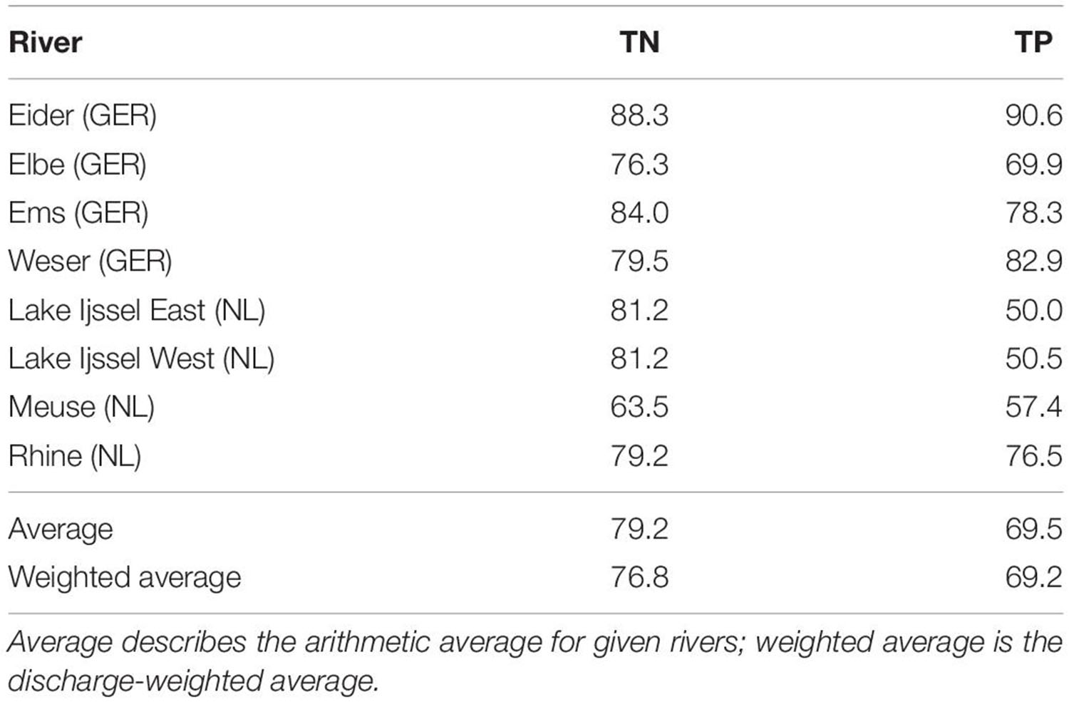
Table 2. Percentage reduction between MONERIS estimate for historic state and measured concentrations based on the ICG-EMO database for the period 2006–2014.

The “Hydrological Predictions for the Environment” model (HYPE; Lindström et al., 2010; Donnelly et al., 2016) calculates water cycle and quality for various regions around the globe, from which we used the application to Europe (thus, E-HYPE). We calculated the discharge-weighted change between 1900 and the control run and applied the reduction value for each river.

Both GPM and ECOHAM require specification of organic (ON and OP) and dissolved inorganic (DIN and DIP) forms of N and P in rivers. Historic estimates were available only for total nitrogen (TN) and total phosphorous (TP) from E-HYPE and TN, DIN, and TP from MONERIS (Gadegast and Venohr, 2015). The historical estimates for DIN and TN by MONERIS correspond to very similar reductions in DIN and ON for most rivers (Kerimoglu et al, 2018; Table 2). We therefore assumed that the reductions in DIN and DIP are equal to those in ON and OP, and we calculated these based on the reductions in TN and TP. As in Kerimoglu et al (2018), considering the loss of historical denitrification potential of major estuaries like Rhine and Elbe (e.g., de Jonge and de Jong, 2002; Dähnke et al., 2008) that have not been taken into account, we assumed 50% lower TN concentrations, reflecting an upper limit for N removal in estuaries (Seitzinger, 1988).

We use EMEP data of atmospheric nitrogen deposition with their original load information for the control run. For the historic scenarios the data are scaled to estimate values back to 1880 (1900 for the E-HYPE run) based on the method described in Schöpp et al. (2003), which were applied in the same form for both scenarios. More details on this method are given in Große et al. (2016).

Variables and Evaluation Areas

For the assessment, we calculated the OSPAR eutrophication indicators (OSPAR, 2003) of dissolved inorganic nitrogen (DIN as sum of nitrate, NO₃, and ammonium, NH₄) and phosphorous (DIP as phosphate, PO₄) and chlorophyll-a (CHL) standing stock. In ECOHAM, we derived CHL from phytoplankton carbon concentration using a fixed CHL:C ratio of 50 mg Chl (g C)^–1. GPM estimates CHL prognostically, based on a photo-acclimation scheme (Kerimoglu et al., 2020).

DIN and DIP concentrations are calculated as average winter values from December to February and CHL as average concentration over the growing season (shortly “summer” hereafter) from March to September following OSPAR definitions. Changes in phytoplankton in the rivers due to the scenarios are not taken into account, however the phytoplankton biomass from the rivers enters the models as detritus contribution. The model results were assessed for the years 2006–2014, but the sensitivity of the results to different definitions of seasons and year intervals was also tested. When comparing the results averaged for the intervals 2002–2008 and 2009–2014, the largest differences occurred for DIN, but these were still insignificant (<5%). When the winter season included November according to the WFD definition (European Commission, 2003), winter nutrient concentrations were not significantly affected (<1%). When the growing season included October according to the WFD definition (European Commission, 2003), largest differences occurred at ECOHAM (up to 9% higher), whereas excluding March (e.g., as in Kerimoglu et al, 2018) led to CHL differences of max. 4% (higher or lower, depending on the model). However, none of these differences affected the findings of the presented study qualitatively.

The OSPAR Hazardous Substances and Eutrophication Committee (HASEC) has agreed on adopting the subdivision of the North Sea based on ecologically relevant assessment areas, as established in the JMP-EUNOSAT project (Enserink et al., 2019; EUNOSAT report) with some adaptations, but the process is not entirely finished. We use the latest shapefile (version COMP4 v7e) that represents the current setup of these assessment areas as provided by OSPAR ICG-EMO in August 2020 (Figure 2).

FIGURE 2

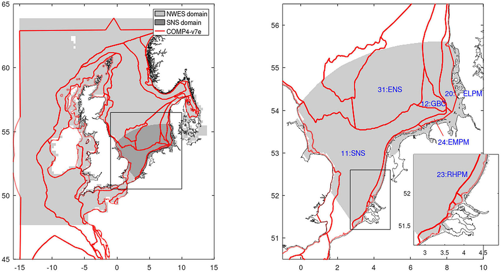
Figure 2. Assessment areas as defined for the eutrophication assessment by OSPAR (solid lines; COMP4 as of August 2020). In gray shades, the model extents of ECOHAM (left panel) and GPM (both panels) are given. The right panel shows the focus region of the central and Southern North Sea including numbers and acronyms of analyzed COMP-areas: SNS, Southern North Sea; ENS, Eastern North Sea; GBC, German Bight Central; RHPM, Rhine plume; EMPM, Ems plume; ELPM, Elbe plume.

Simulations and Analysis

We simulated with both model systems the current state of the ecosystem as a Control run “C” for the years 2006–2014 (with eight years spin-up prior to this period) for comparison with the historical state. To represent the historical scenarios based on MONERIS (“M”) and E-HYPE (“E”), we applied the same physical forcing, but adapted the nutrient loads to historical status (see section “Reconstruction of the Historical State”). Hereafter, we refer to “model” as the biogeochemical models ECOHAM and GPM and to “scenarios” distinguishing simulations using river loads based on MONERIS and E-HYPE (though these are models themselves).

To compare changes in concentrations of DIN, DIP, and CHL, we calculate the percentage difference for the analysis. Thus, in section “Historical State According to the Two Scenarios” the percentage deviation of control concentrations (C) from historic state (H_E and H_M) are calculated as:

$$\mathrm{\Delta }{}_X=(H{}_X-C)/C\times 100,withXforMONERIS$$

$$\mathrm{}and\text{E-HYPE}$$

We normalized the absolute differences in historic concentrations as estimated by E-HYPE and MONERIS also by the control concentration C to compare better the scenario uncertainty:

$$D=(H{}_E-H{}_M)/C\times 100.$$

Quantifying Variability

To quantify different sources of uncertainty we considered the lateral, seasonal and inter-annual variabilities for both scenario runs for each model. To achieve this, we calculated in a first step the daily mean concentration for DIN, DIP, and CHL resulting in a time series of daily values for 2006–2014 at each horizontal grid cell for each simulation. To quantify the seasonal variability, we calculated the seasonal variance (winter for nutrients and summer for CHL) for each year and then the average standard deviation across years for each grid cell. For the inter-annual variability, we first calculated the inter-annual variance for each day and from this the average standard deviation within the season on the model grid. Additionally, we calculated the seasonal mean concentration for each assessment area (see section “Variables and Evaluation Areas”) as climatology for each cell on a refined high-resolution grid. Finally, we calculated the standard deviation within the assessment area (representing the lateral variability).

The main objective is to gain insight into the significance of the differences emerging through the use of different biogeochemical models (GPM and ECOHAM) and historical riverine loading scenarios (MONERIS and E-HYPE), in relation to these natural sources of variability, and how these relations vary in different regions. This means that we first look at the differences in the mean concentrations between the scenarios for each of the two models, and then relate these differences to the variability represented by the related standard deviation. For better comparability, we calculate the percentage deviation as standard deviation relative to mean value for each source of variability as well as between models and scenarios.

Results

Current State According to the Two Biogeochemical Models

First, we investigated the differences in the model setups to reproduce the nutrient distributions in the control run “C” (Figure 3). The average spatial patterns over years 2006–2014 for respective seasons estimated by the two models are similar: Winter DIN and DIP are highest in the coastal region (exceeding 10 mmol N m^–3 and 1 mmol P m^–3 for DIN and DIP, respectively) with maxima close to river outlets of rivers Thames, Rhine, Weser, and Elbe. Nutrient concentrations decrease in the offshore region to 3–5 mmol N m^–3 and 0.4–0.5 mmol P m^–3. For the summer standing stock of CHL, the coastal concentrations exceed 4 mg Chl m^–3, while in the open North Sea these are below 3 mg Chl m^–3. Differences between model estimates exist as well: GPM shows a more distinct near-shore nutrient front. In the offshore zones, differences are less pronounced. Nearshore DIN and CHL concentrations estimated by GPM are overall higher, while ECOHAM estimates higher offshore DIP concentrations.

FIGURE 3

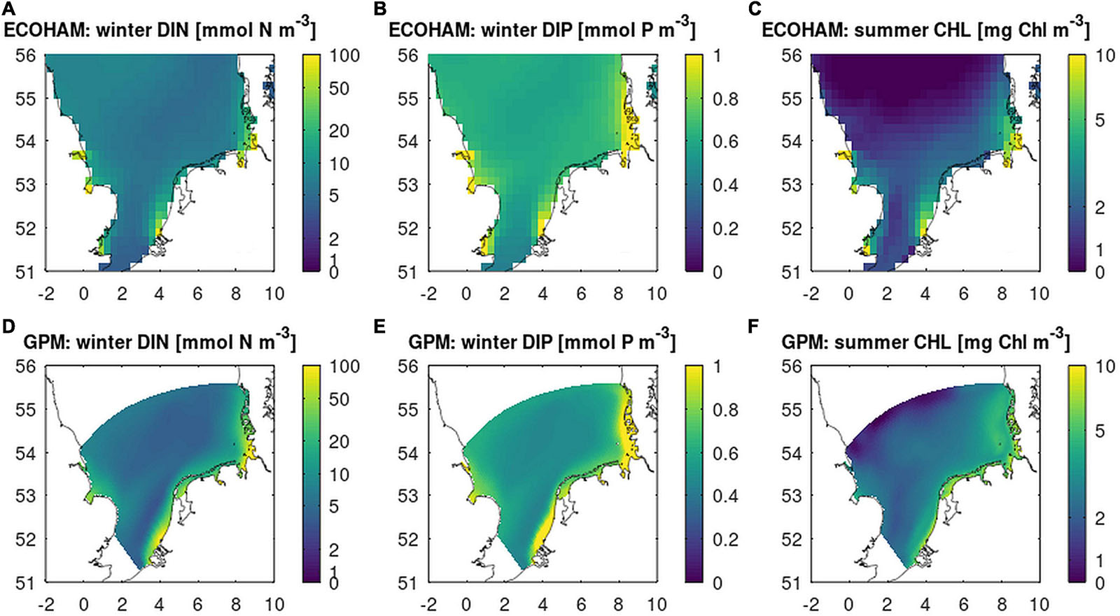
Figure 3. Results from the Control run (“C”): DIN (A,D), DIP (B,E) concentration as December–February average, and CHL (C,F) concentration as March–September average from ECOHAM (A–C, upper panel) and GPM (lower panel, D,E). DIN and CHL colors are on a log₁₀ scale.

Historical State According to the Two Scenarios

The historical nutrient input estimates from MONERIS for the Dutch and German rivers are reduced by 76.8% for TN compared to the control run (Table 2). This is substantially above the reduction estimated by E-HYPE (63%; Table 3) for these rivers. For TP the difference between the two catchment models is even more pronounced: while MONERIS estimate of the historic state corresponds to, on average, 69% reduction (Table 2), the average estimated reduction of E-HYPE is 45% (Table 3), i.e., a difference of 24% relative to the current conditions.

TABLE 3

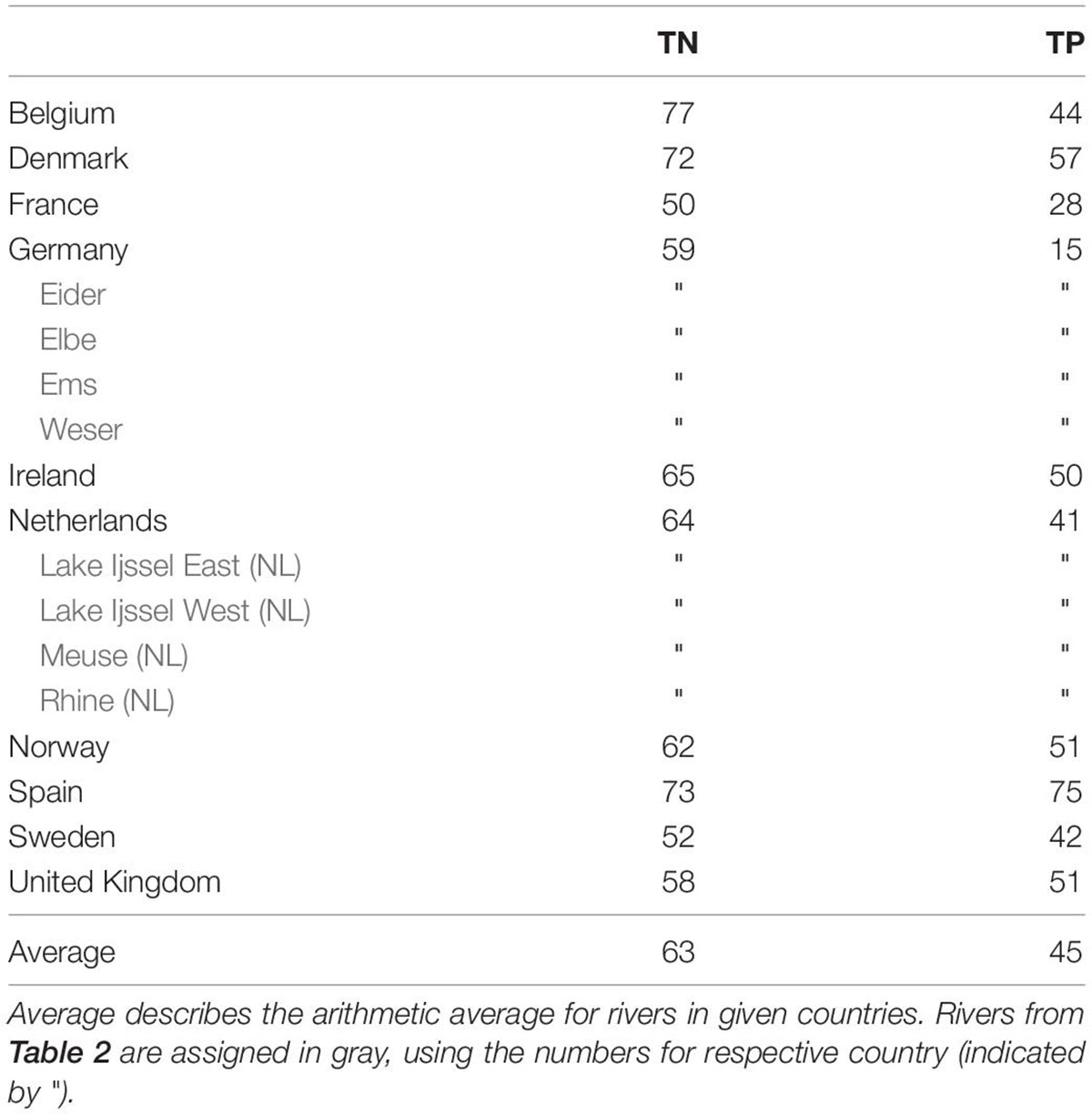
Table 3. Percentage reduction between E-HYPE estimate for the historic state and measured concentrations based on the ICG-EMO database for the period 2006–2014.

The response from the average (2006–2014) values of DIN, DIP, and CHL as obtained by GPM to the reductions in riverine loadings based on MONERIS and E-HYPE historic estimates are shown in Figure 4. In comparison to the control run, DIN shows for both catchment models the largest reductions in the range of 50–90% except for the north-western model region (Figures 4A,D). For DIP, reductions are below 20% for most of the model domain with larger reductions only in the coastal regions (Figures 4B,E). For CHL the changes compared to the control run are less pronounced than for nutrients. Changes reach 20–50% in the coastal region but are <10% in the offshore region, decreasing toward the north-western part of the model domain. In this area, the CHL concentration is higher in the historical run compared to the control run (Figures 4C,F). This increase is due to the combination of surplus Si in the historic state (as a result of earlier N and P depletion), and the maintenance of low N-limitation in this area, driven by the relatively high DIN concentrations prescribed at the boundary, resulting in a southward N-flux governed by the dominant circulation pattern (results not shown). Based on both scenarios, the change of CHL concentration in the river mouth zones of Rhine and Elbe are less changed than in the other coastal regions (<20%), which is more pronounced in the comparison for the E-HYPE scenario.

FIGURE 4

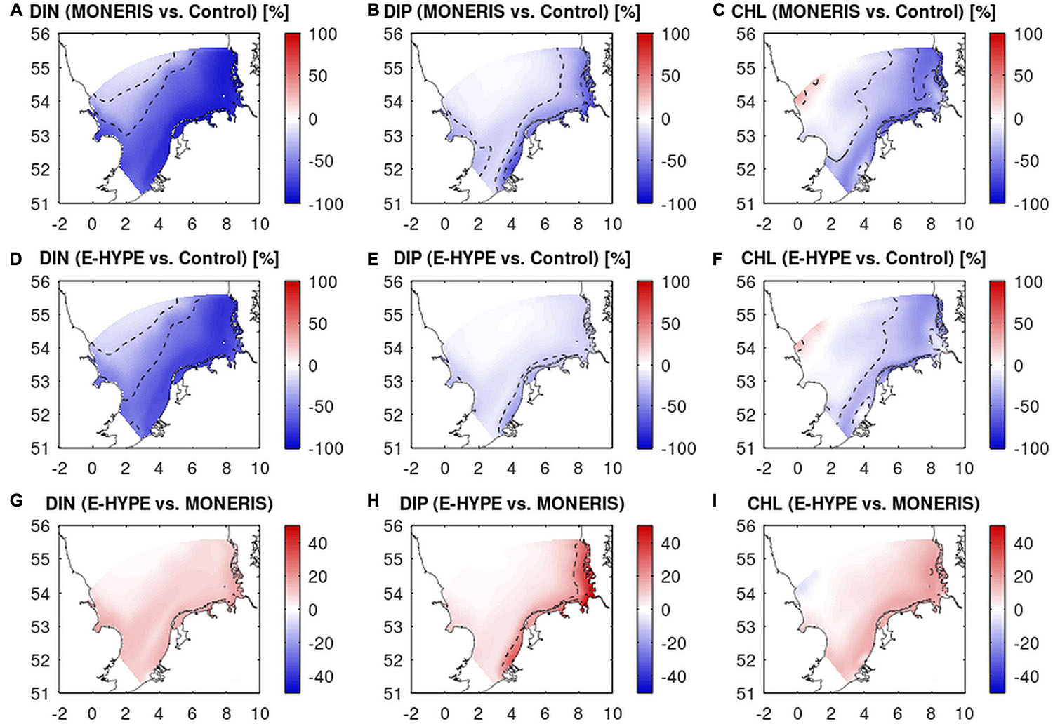
Figure 4. Percentage change between historical run (“H”) and control run (“C”) from GPM based on river discharge from MONERIS (A–C) and E-HYPE (D–F) as Δ_X = (H_x – C)/C × 100, where H_X and C stand for the concentration of each variable [DIN (left), DIP (center), and CHL (right)] in the Historic (X for MONERIS and E-HYPE) and Control state C, averaged within the respective seasons. (G–I) Percentage difference between concentrations according to the two historical scenarios normalized by the control run (C_E – C_M)/C_C × 100. Dashed lines indicate the 20 and 50% isolines. Mind the different color scale for the lower panels.

To understand better the differences in the projections according to the two historical scenarios, we calculated D, defined as the percentage difference of historic concentrations based on E-HYPE from those based on MONERIS, relative to the control concentrations. Reductions of all three variables are overall larger based on MONERIS compared to using E-HYPE, i.e., concentrations in the historical scenario based on E-HYPE are higher (Figures 4G–I) and D is positive. D is largest for DIP, reaching 50% in the coastal region (Figure 4H), whereas in the offshore region D of DIN is more pronounced, though for both nutrients the difference is low (<20%), decreasing toward Northwest reaching zero north of the Dogger Bank. Like for nutrients, CHL is higher in the E-HYPE scenario than in the MONERIS forced run, though its D-value in the coastal zone is less pronounced than for nutrients especially in the vicinity of the Rhine and Elbe inlet and remains below 20% (Figure 4I) throughout the model domain. The results based on ECOHAM are qualitatively comparable for nutrients and thus not shown here (but are available in Supplementary Figure A1). However, for CHL ECOHAM shows largest differences in simulations from MONERIS and E-HYPE in the Weser and Elbe region (Supplementary Figure A1I) in contrast to the minima calculated with GPM.

Internal Sources of Variability Within Assessment Areas

We compare (Figures 5, 6) the outcome of the two scenarios for each of the two model applications against different variability ranges as described in section “Quantifying Variability.” Here, the mean represents the average concentration for each assessment area. This value is independent of the analysis of the variability, i.e., it is identical in all categories of variability (for all bars of the same color). For the representation of the variability, we considered three categories of variability: lateral (within each area), seasonal and inter-annual. The given numbers in Figures 5, 6 indicate standard deviation as percentage of the mean to obtain comparability between the parameters.

FIGURE 5

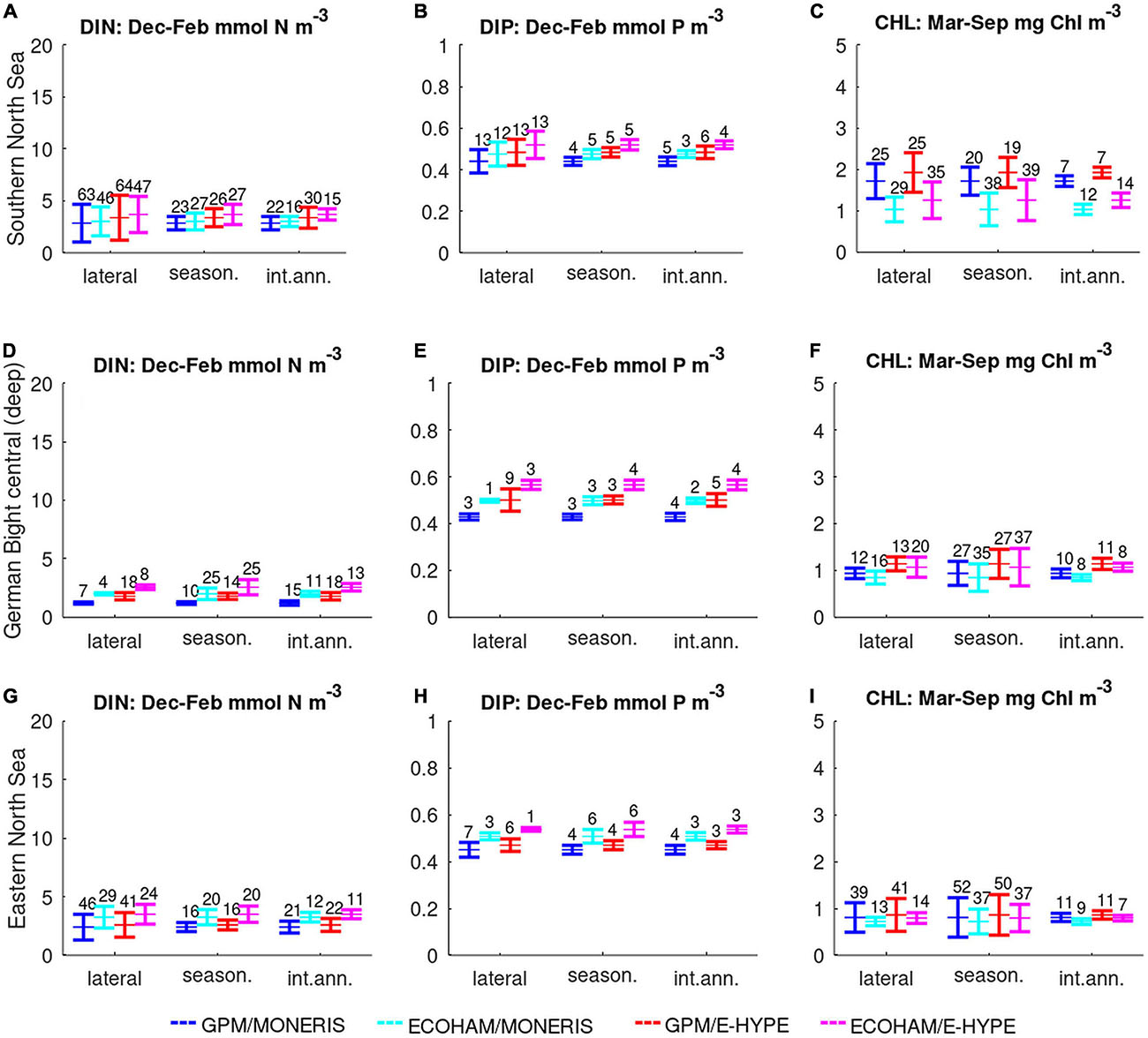
Figure 5. Bar-plots of mean and standard deviations for each biogeochemical model (GPM: bars 1 and 3; ECOHAM: 2 and 4) and hydrological model (MONERIS: 1 and 2; E-HYPE: 3 and 4) based on lateral, seasonal, and inter-annual variability in three off-shore areas (from top to bottom): Southern North Sea (A–C), German Bight (D–F), and Eastern North Sea (G–I). Numbers above the bars indicate relative variability (i.e., SD/mean × 100).

FIGURE 6

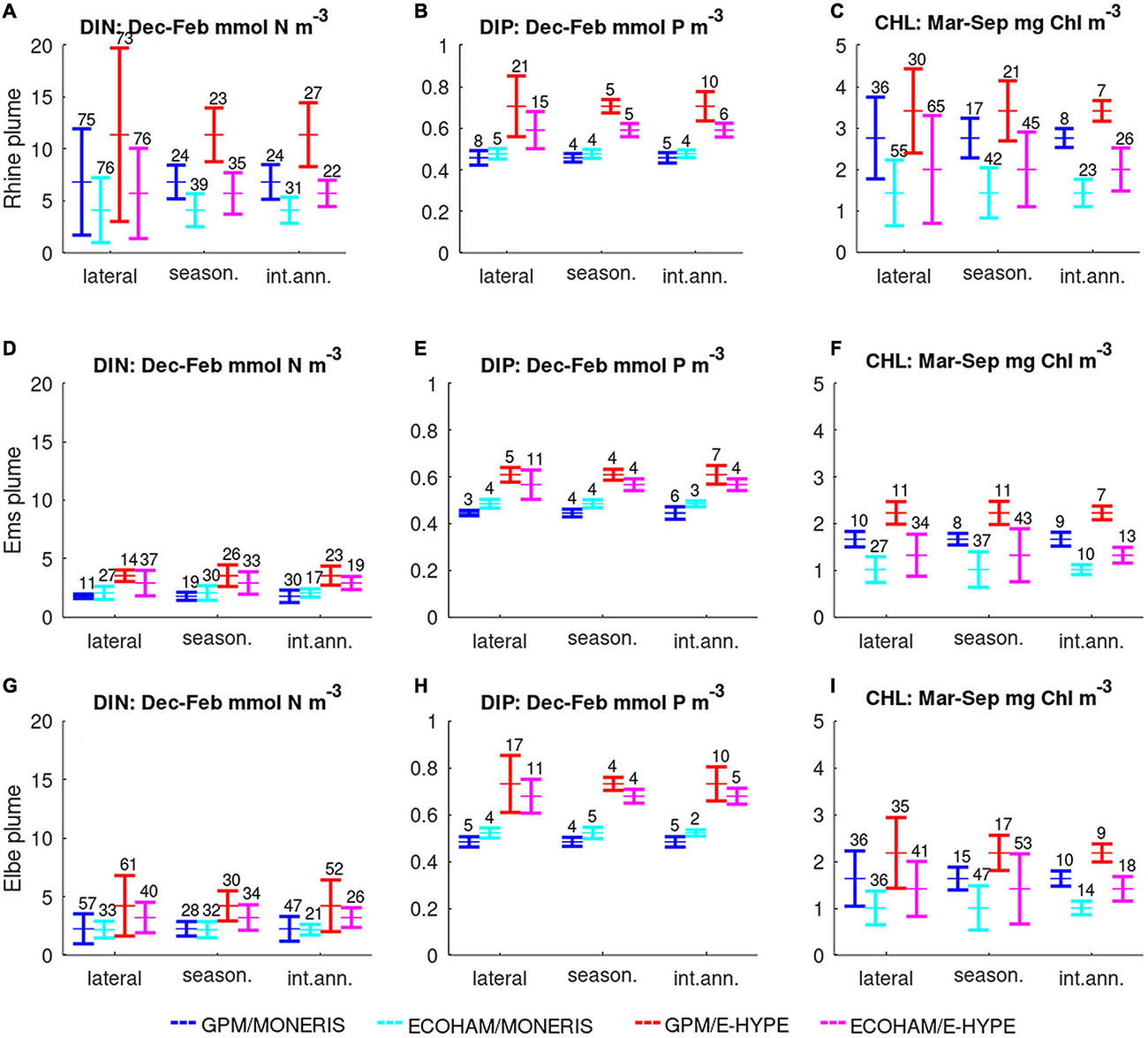
Figure 6. Bar-plots of mean and standard deviations for each biogeochemical model (GPM: bars 1 and 3; ECOHAM: 2 and 4) and hydrological model (MONERIS: 1 and 2; E-HYPE: 3 and 4) based on lateral, seasonal, and inter-annual variability in three river plume areas (from top to bottom): Rhine plume (A–C), Ems plume (D–F), and Elbe plume (G–I). Numbers above the bars indicate relative variability (i.e., SD/mean × 100).

The results for three offshore areas are shown in Figure 5:

Southern North Sea area (No. 11, SNS): The water in this assessment area is influenced by the English Channel and covers most of the western part of the Southern North Sea, reaching up to the Humber plume. The mean concentrations are similar for both scenarios for DIN and DIP, while CHL estimates from GPM are significantly higher than those of ECOHAM. Because of the large extent, the lateral variability in nutrients is higher than temporal variabilities in both models: Lateral variability for DIN exceeds 60% in GPM and 45% in ECOHAM for both scenarios, while for DIP both models reach 12–13% for each of the scenarios. The variability of CHL is similar for lateral and seasonal variability: Deviations in GPM are 25% for lateral compared to 19–20% for seasonal variability. ECOHAM shows larger variability with seasonal variability (38–39%) exceeding lateral variability (29–35%).

German Bight central (No. 12, GBC): The German Bight area has a triangular shape and represents the deep Elbe channel extension. In general, the differences in all four simulations are small. The results are more sensitive to the river load estimates than to the biogeochemical model. One exception are the higher mean values for the E-HYPE scenario. The difference between the mean values for the models and the scenarios are small for DIN and larger for DIP, while the results for CHL are similar. The variability for DIN and DIP is small except for the lateral variability of the GPM/E-HYPE. For CHL, the highest variability is in the seasonal component.

Eastern North Sea (No. 31, ENS): The Eastern North Sea area represents a region east of the Dogger Bank, which reaches up to the northern tip of Denmark. The area is characterized by offshore conditions, but is most susceptible for oxygen depletion events because of its shallow depth. Small but obvious differences can be seen between scenarios and models for DIN and DIP, but these differences vanish for mean chlorophyll concentration. For DIN, these differences are within the range of the lateral variability for all model simulations, while for DIP we found distinct difference between the two GPM simulations and those from ECOHAM. For CHL the seasonal variability is largest, followed by the lateral variability for the GPM model results in both scenarios.

Overall, the variability is within 3–64% for all scenarios and areas and generally highest for DIN. The differences between mean concentrations among the biogeochemical models and the two scenarios are mostly <10%. In addition to these offshore regions, we compared three river plume areas, which results we show in Figure 6:

Rhine plume (No. 23, RHPM): This area does not cover the region of the direct Rhine input but corresponds to the narrow coastal part along the Dutch coast up to Texel Island. There are large discrepancies between the mean concentrations of the different scenarios and models. The lateral variability is high for all variables, but most prominent for DIN (73–76% for all models/scenarios). Therefore, the lateral variability covers a larger range than the differences between the mean concentrations for the different models and scenarios. For the seasonal and inter-annual variability, this is not the case. For DIN and DIP the differences of mean concentrations between the models and scenarios exceed the seasonal and inter-annual variability. For CHL, mean values are higher for the E-HYPE scenarios compared to respective MONERIS-based runs with both biogeochemical models for all variables, while both GPM simulations reveal higher concentrations than the ECOHAM runs except for DIP using MONERIS. ECOHAM shows higher variability in CHL (23–65%) than GPM (7–36%). However, the differences in the mean values for the models and the scenarios are larger than this range of variability.

Ems plume (No. 24, EMPM): This area corresponds to the narrow coastal part between the two large rivers Rhine and Elbe. The mean nutrient concentrations show a clear distinction between the scenarios but are close for the two models. The overall variability is much less than in the Rhine river plume area. Higher variability can be seen for the lateral and seasonal variability for CHL, especially for the ECOHAM model results.

Elbe Plume (No. 20, ELPM): The key results in the Elbe plume area, extending along the North Frisian and Danish coast, are similar to the Ems area, as the simulations with E-HYPE have higher concentrations than those with MONERIS, especially for DIP (Figure 6H). These differences between the scenarios for DIP are much larger than all the related variability plots. For CHL, we see the same pattern as for nutrients, but the differences between models are larger. The most prominent source of variability in DIN is the spatial component of about 60% for GPM in both scenarios (35–40% with ECOHAM). Here the lateral variability covers the range between the mean for the different scenarios. For DIP, the variability is about 5% for most runs, except for lateral variability of both models (10–18%). Even though the lateral variability is high for the E-HYPE scenario in both models, it does not cover the mean values from the MONERIS scenario. For CHL, the variabilities differ between models: While with GPM the lateral variability is highest at 35%, at ECOHAM this component is similar, but seasonal variability is dominating at 45–50%. Here, the differences between the models are larger than the respective variability. Nevertheless, the larger phosphorus reduction generally results in lower CHL values for both models in the MONERIS scenario.

The river plume regions have higher mean values as well as larger variability in comparison to the offshore regions as shown in Figure 6. In these regions, also the differences between the two models and the two historical scenarios become more prominent. Overall, the variability was larger in ECOHAM in the plume regions, while GPM showed more often larger variability in the offshore regions, specifically for the inter-annual variability of nutrients. The differences in variability were also broader in the coastal regions when comparing simulations with the two biogeochemical models. In contrast, for simulations using MONERIS or E-HYPE variability was similar. Concerning the mean values, simulations with E-HYPE resulted in higher concentrations than those with MONERIS.

Inter-Comparison of Uncertainties Against Internal Sources of Variability

Based on these findings, we relate the sources of internal variability (lateral, seasonal, and inter-annual) to the variability between the models and the river input scenarios (Figure 7). This comparison shows that lateral variability is most often the largest source (indicated bold in Supplementary Table A1), followed by variability through river scenarios and models. Seasonal variability has a secondary influence, while inter-annual variability is least in most cases. However, the sources are differently distributed among indicators: For DIN, lateral variability is the most prominent source, while seasonal and river variability are less. In contrast, for DIP the river loads induce the largest variability with lateral being less notable. For CHL lateral and seasonal variability are similarly large. Among the river plume areas, we find distinct differences specifically between the Rhine plume area (21, RHPM) and the Elbe plume area (20, ELPM), two major rivers entering the North Sea, that shape the nutrient dynamics of the south-western North Sea. The Rhine plume area has the highest variability that is mostly pronounced for the lateral variability. Differences between the two scenarios or simulations are relatively lower, indicating that the natural variability exceeds the respective model uncertainties. The Rhine plume area shows the largest variability for all indicators, followed by the Elbe plume and the SNS (see Supplementary Table A1 for the numbers).

FIGURE 7

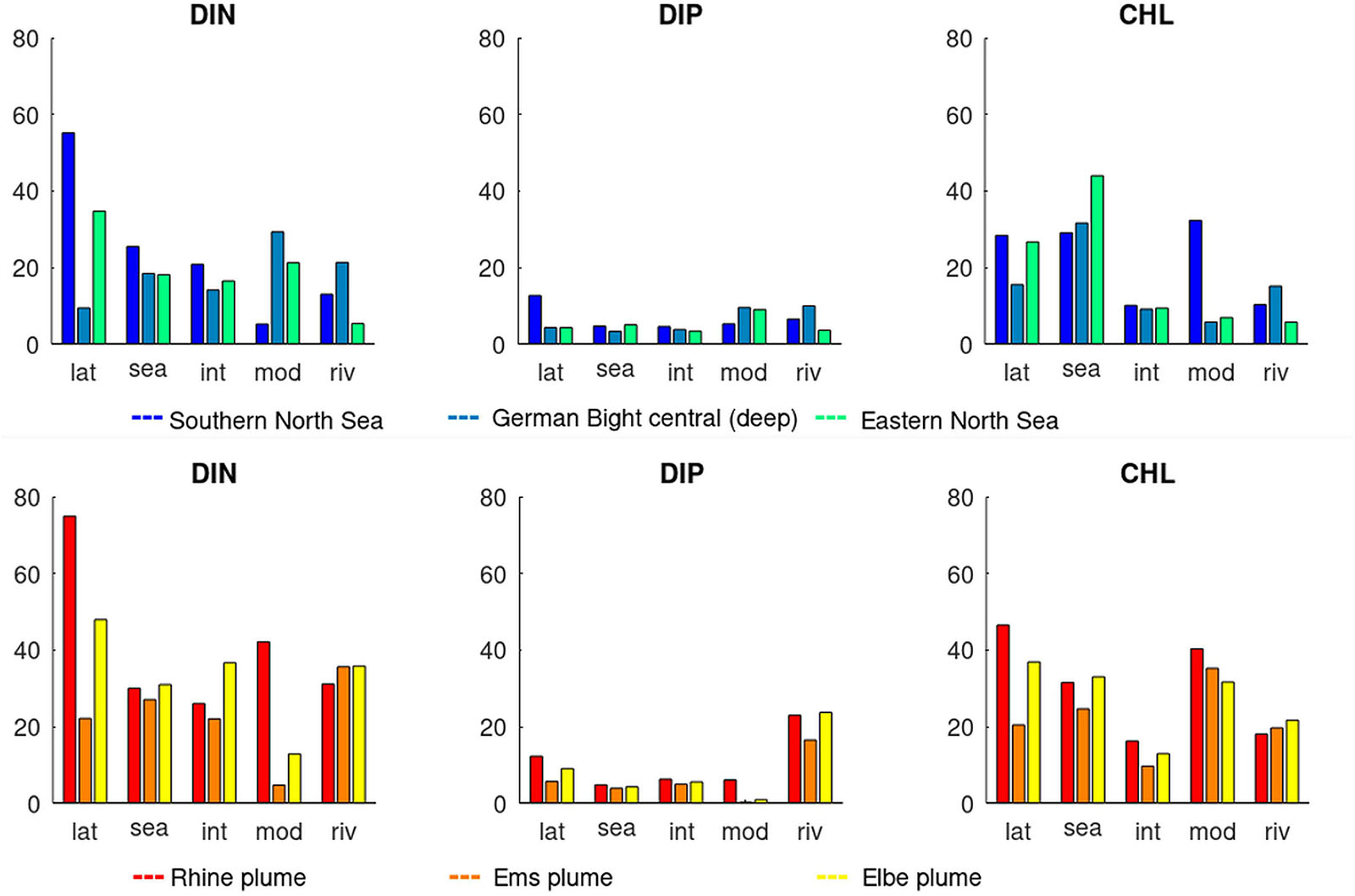
Figure 7. Comparisons of sources of variability (lateral, seasonal, inter-annual, model, and river scenario) of DIN, DIP, and CHL in six assessment areas. Top: offshore-regions Southern North Sea (blue), German Bight (turquoise), and Eastern North Sea (green). Bottom: coastal plume regions Rhine (red), Ems (orange), and Elbe (yellow). Variability is given as standard deviation normalized by mean values (as percentage).

Discussion

To assess the health of an ecosystem, establishing reference conditions is important (Borja et al., 2012). While biogeochemical models are considered as useful tools to meet this objective, various sources of uncertainty pose challenges to obtain reliable and representative model-based projections. Among a number of potential sources of uncertainty, the presented study focused on the impact of the model representation (both on the grid resolution and the description of the biogeochemical processes like phytoplankton growth) of the physical-biogeochemical model, and the riverine loading scenarios, which were used to obtain the model-based reconstruction of the historical (i.e., pre-eutrophic) state of the North Sea. Here, we discuss some specific findings before we analyze in more detail the relevance of the river load scenarios (see section “Relevance of the Riverine Loading Scenario”), the biogeochemical models (see section “Relevance of the Biogeochemical Model”) and the uncertainty from the different simulations (see section “Importance of Model-Based Uncertainties Relative to Internal Sources of Variability”), and giving some suggestions for future studies (see section “Suggestions for Future Modeling Studies”).

First, reductions of the historic state as estimated by the two catchment models, MONERIS and E-HYPE, are more pronounced for TP (69.2 vs. 45%) than for TN (76.8 vs. 63%, see Tables 2, 3). The disparities especially for TP between MONERIS and E-HYPE have been found to be related with differences in the representation of the urban population, connectedness to sewage systems and the level of treatment applied (OSPAR ICG-EUT, personal communication). How does this translate into the model results from GPM and ECOHAM?

One interesting feature is that reductions of CHL close to rivers Rhine and Elbe are small, specifically in the simulation using E-HYPE. This is explained by higher DIP concentration in the E-HYPE scenario that promotes phytoplankton growth, whereas P-limitation is more pronounced in the MONERIS simulations.

For ECOHAM, this follows a picture that has been described in Emeis et al. (2015) where a major reduction within the vicinity of the Rhine and the Elbe could only be achieved by an additional reduction of DIP. In contrast, the GPM model reacts to the general reduction in both scenarios nearly in the same way for CHL, resulting in nearly no contrast for these areas in the comparison of the river input scenarios (Figure 4I). These differences compared to the control simulations help to understand the state of the pre-eutrophic North Sea.

Second, when models are used for projecting the state of a system under different (past or future) conditions, various sources of uncertainty become relevant: specific models used, definition of scenarios, or the interaction with other models, if these are used as “forcing.” It is often not straightforward to evaluate the relative importance of these various sources of uncertainties, and to decide how significant they are. Here, we aimed to consistently quantify these uncertainties in terms of variability, and assess their importance by comparing these to the internal sources of variability (Figure 7). Pappenberger and Beven (2006), in the context of hydrological modeling, address the importance of naming uncertainty of modeling studies in (political) decision-making. Allen et al. (2006) describe different methods to quantify uncertainty as a means of (single) model validation (against data). Here, we consider three sources of internal variability: lateral (spatial), (intra-) seasonal, and inter-annual, and we assess these in various COMP-areas for each variable: DIN, DIP, and CHL.

The isolines of DIN and DIP in general, with an exception of the E-HYPE scenario from GPM, are related to the small band of Elbe dominated water, which can be seen in the analysis from Lenhart and Große (2018; Figures 4A,B). The variability analysis for the Ems plume (Figures 6D–F) provides a similar picture, only with a reduced variability for CHL. The generally low variability can be related to the fact that the area is rather narrow along the East Frisian coast. In the German Bight area, the differences in all four simulations are small, even though the assessment area represents a region with distinct gradients from the coast to the offshore regions. This indicates that this area represents a rather homogeneous water body.

For the Rhine plume (Figures 6D–F), the differences between the two scenarios are large for all displayed concentration and comparable with the differences between the models. Here, the wide range within the DIN concentrations stands out, especially within the lateral variation, compared to the rather narrow band for DIP. From our analysis, we could not distinguish, whether this is related to the narrow coastal region this area represents or variations in the nitrogen load of the Rhine. As a result, the lateral variations within CHL are substantial, and cover a wider range than the differences between the scenarios and the models. Despite the large extent covered by the SNS area (area 11), including a coastal gradient in the parameters, we found only small variability, except for the lateral variability in DIN. This can be explained by the influence of a large varying nitrogen transport from the Rhine plume, which also influences the variability in the lateral and seasonal CHL concentration.

Relevance of the Riverine Loading Scenario

Since the WFD as well as the MSFD demand a historic perspective for the definition of the “pre-eutrophic” state of the marine environment, the question remains how to achieve estimates of the nutrient loadings associated with these (historic) conditions. So far, only one method is known for the North Sea, which is based on measurements. While making use of the distinctive isotopic signature of river-borne nitrogen, and by reconstructing the isotopic ratios in sediment cores with an ecosystem model, Serna et al. (2010) provided an estimate of the historic state of the system. However, since the sediment core data do not provide information on the relative contribution of different rivers, the authors assumed a uniform level of nitrogen reduction (90% reduction compared to the present loads) in all rivers, which is not necessarily realistic. Some restoration efforts have been done for certain rivers (see Topcu et al., 2011 for an overview), whereas for some others, such efforts have been lacking.

An alternative is applying catchment models, which, for each river, provide nutrient load estimates based on the historical records and estimates of population density and land use. The studies by Desmit et al. (2018) and Kerimoglu et al (2018) followed this approach, based on the estimates by the catchment models “Riverstrahler” focusing on the English Channel/Bay of Biscay regions and “MONERIS,” investigating the SNS region, respectively.

Here, we considered the reductions in river loads as estimated by two different hydrological models, MONERIS and E-HYPE. The calculations from MONERIS are based on historical records, for example on land use, population density and other factors around 1880, which lead to detailed estimates on the historic loads for a number of rivers (Venohr et al., 2011). In contrast, the E-HYPE estimates are based on a spatially large model with assumptions on the reduced impact from point and rural sources, land use and fertilization, which are available for all European river systems around 1900 (Blauw et al., 2019). When comparing the two model approaches, they differ in the per capita production of N and P and in the application of atmospheric nitrogen deposition. Nevertheless, the estimates are comparable for nitrogen, whereas they differ considerably for phosphorus without a plausible explanation so far (see Tables 2, 3). The assumption of nitrogen retention has a significant impact on the actual reduction. Neglecting retention, the average nutrient reduction from the MONERIS reduction estimates would have been 54% in the weighted average (compared to 77% used here). We can conclude therefore that the differences between the years of the application of the catchment models are less than the differences in the methods applied.

In the scenario application of the ecosystem models based on MONERIS input, the simulation results show larger nutrient reductions in comparison to the control run than those using estimates by E-HYPE. Consequently, the simulations using E-HYPE loadings returned consistently higher CHL concentrations than those from MONERIS. In the offshore regions, differences between both scenarios became less pronounced. For nitrogen, the difference between the two catchment models (13%) in river input has translated approximately to the differences estimated for the marine waters, while marine phosphorous concentrations differ clearly. The percentage change in river input differs by about 24%, but increases up to 50% in the North Sea (see Figure 4G). This can partly be explained by the distribution of riverine input. While the average reduction in E-HYPE-based TP-loads is 45%, largest reductions have been estimated for Spain (75%), Denmark (57%), Norway and United Kingdom (51%), and Ireland (50%). Spanish and Irish river discharges hardly influence nutrient dynamics of the North Sea, whereas the influence of Danish (mostly toward the Skagerrak/Kattegat) and Norwegian river outputs is rather limited to the north-eastern part of the North Sea (and not covered by GPM). In contrast, reductions of historical river loads for France (28%), Netherlands (41%), and Germany (15%), which substantially influence nutrient dynamics in the SNS, are significantly lower in the MONERIS scenario.

Relevance of the Biogeochemical Model

When considering the differences between the scenarios and the resulting ecosystem simulation results, applying the same river input scenario to two different models provides an outlook on the differences of the marine model simulation results. Consistent to the variations between the river input scenarios, differences between the models were larger in the coastal regions than in the off-shore areas. CHL concentrations were thereby consistently higher in the river plume regions in GPM than in ECOHAM.

GPM predicts larger cross-shore nutrient gradients, which is owed to the much finer spatial resolution of 1.5–4.5 km along the continental coast. In HAMSOM/ECOHAM the mesh size of 20 km restrains the model from resolving the coastal zone and supports increased mixing with inflowing Atlantic water from the English Channel. The similar concentrations in the offshore regions as estimated by GPM and ECOHAM are as expected, given that GPM uses boundary conditions for dissolved inorganic nutrient, dissolved organic material and detritus pools estimated by ECOHAM, and suggest that the resolution of ECOHAM is sufficient for simulating these regions. Slightly higher offshore nutrients in ECOHAM may be due to the differences in the parameterization of limitation and plankton stoichiometry. ECOHAM uses a fixed N:P ratio for phytoplankton, while GPM represents prognostic variables for phytoplankton-N and -P.

In general, one can conclude from the scenario simulations presented here that differences between the biogeochemical models were smaller than the differences between the historic input scenarios (Figure 7). This can be attributed to the fact that both models have been validated and thus general structures are similar. Thus, biogeochemical model-based uncertainties are rather structural – defined by Arhonditsis et al. (2008) as difference in equations as described above, rather than input uncertainties.

Importance of Model-Based Uncertainties Relative to Internal Sources of Variability

For most instances, we found that within the single scenarios, the variability among the three analyzed eutrophication indicators is least for DIP and that lateral variability is highest for the nutrients, while for CHL the seasonal variability is similar or higher than the spatial one (Figure 7). Since CHL undergoes a distinct seasonal cycle of spring bloom, summer depletion and fall bloom, the maximum CHL concentration as considered by the OSPAR Common Procedure (OSPAR, 2003) is a useful supplementary indicator.

In the SNS (11, “SNS” in Figure 2), the largest considered assessment area, lateral variabilities are largest, compared to the other offshore areas. These can be explained by the considerable salinity gradient in this region (Desmit et al., 2015). In contrast, the German Bight central area (12, GBC) is less affected by this lateral variability.

The lateral variability depends on how homogeneous the water mass is reflected by the assessment area definition. This is not only related to typical water mass characteristics, like temperature and salinity, but also to homogeneity in the overall environmental parameter like SPM which in relation to the light limitation can govern the response of CHL to historic reduction levels in the riverine nutrient input. Different levels of DIP reduction can cause variations in the resulting response of the CHL concentration especially within the vicinity of the major rivers entering the North Sea like Rhine and Elbe. These differences have been shown to be larger than the differences in the model representation.

In this context, the question arises in which way the OSPAR definition of the time intervals representing “winter” for nutrients and “growing season” for CHL have influence on the outcome. However, our analysis with different time intervals showed no significant influence on the outcome of each of the tested scenarios (see Supplementary Tables A2, A3). Some changes can be related to differences in the biogeochemical models, like those found for changes in variation of growing season: ECOHAM showed a more pronounced fall bloom with increased concentrations in October as well as the bloom in March compared to GPM. The effect on nutrient levels was similar in both models and reduced values is expected with nutrients depleted at that time. Variation in the period had no significant impact supporting to use shorter periods, which can save on computational time and effort.

The variables we focused on in this study, DIN, DIP, and CHL, all represent concentrations that can be easily compared to observations. As such, they have been also selected by OSPAR as assessment indicators. However, these variables are not necessarily the most representative of the ecosystem functioning or most comparable between different modeling approaches. For instance, CHL can acclimatively respond to changes in light or nutrient availability, and this can significantly modify the apparent eutrophication response (Kerimoglu et al, 2018). Moreover, modeled CHL can be strongly sensitive to “cosmetic” assumptions that do not affect any other modeled quantity, such as CHL:C ratio being a certain fixed factor (like in ECOHAM). In contrast, Net Primary Production (NPP) is more directly related with the functioning of an ecosystem, and the model estimates are more robust. It should be noted that the mean NPP estimates of different models can not be expected a priori to be similar relative to their CHL estimates: depending on the prevailing environmental conditions, the variability in NPP can be indeed smaller than CHL (e.g., lateral and between model variability in the Rhine Plume, compare Supplementary Figure A2B vs. Figure 6C), but they can also be larger (e.g., between-model variability in the Eastern North Sea, compare Supplementary Figure A2E vs. Figure 5I). However, due to the scarcity of respective observation data, skill of models are often not evaluated with regard to such alternative quantities like NPP.

When it comes to the use of the model simulation for decision support, the question of the reliability of the model results is equally important as a transparency of the processes within the model simulation. Even well validated models provide different results for different regions, despite the fact that the setup was carefully planned, like the use of common river loads, boundary condition, and atmospheric nitrogen deposition. It needs to be pointed out that in model comparison studies the fact of nudging of boundary to models that cover smaller domains is an important aspect to include effects of river nutrient load reduction from sources that are outside their own domain (Lenhart et al., 2010). Only by nudging the boundary condition the comparability of the results within the smaller domains in comparison to the wider domain models can be guaranteed, which is an important aspect in the use of the model results as the basis for deriving threshold values. It should be noted that this introduces some dependency between the models we used: if we had compared two entirely independent models (i.e., no exchange of information at the boundaries), the variability among the models (Figures 5–7) might have been larger.

Suggestions for Future Modeling Studies

In the current study, we aimed to gain an overview of the relative importance of uncertainties related to model choice and scenario definitions, and evaluate the importance of each in various assessment regions. It is possible to refine such comparisons further to the level of sub-modules or individual process descriptions or specific assumptions, to assess their relevance in particular. Modular schemes that allow coupling various model components (see, e.g., Bruggeman and Bolding, 2014; Lemmen et al., 2018) would facilitate such a task.

In addition to the changes within the eutrophication indicators, one also want to have a deeper understanding of the contributions from different riverine sources in relation to the newly defined assessment areas. For this purpose, the so-called “trans-boundary nutrient transports” (TBNT) approach provides a method for the tracing of an element, like nitrogen, from individual sources throughout the entire biogeochemical cycle, including the physical transport processes (Ménesguen and Hoch, 1997). By the use of this method, the relative contribution of river loadings can be quantified for different regions (e.g., Lenhart and Große, 2018).

An established method for coping with the difference between model results is the application of the so-called “weighted ensemble modelling.” In a first step, the ensemble means are calculated, and then each ensemble member can be weighed based on its skill score (e.g., Skogen et al., 2014). This skill score is usually based on a cost function, which judges the performance of one model output on some key parameter vs. in situ data. While this method is well established within the hydrodynamical modeling community, the drawback for its use in ecosystem modeling application is the amount and especially the spatial coverage of in situ data that are needed.

The findings from this study show different sources of variability in biogeochemical model simulations. When using such models for the projection of future or target states, further sources need to be considered: temperature, which is projected to further increase in the future, is a main factor for the timing of the spring bloom (Wiltshire et al., 2015). Additionally, other influences such as changes in the food web can further influence the peak as well as regional differences of the spring bloom (Mills et al., 1994). Such changes in the ecosystem structure can be further sources of variability and need to be captured by biogeochemical models.

Conclusion

In this study, we considered different influences that can affect the simulation of the pre-eutrophic North Sea, which shall provide a basis for estimating the reference state and GES thresholds. Since the available reductions provided by both catchment models differed considerably both for TN and even more in TP, we analyzed these differences in the context of the internal variability and in comparison to two biogeochemical models.

Our results show that (i) both, the biogeochemical models and the hydrological models have an impact on the nutrient and chlorophyll-a levels, but less than lateral and seasonal variability, in general; (ii) close to the regions of freshwater influence (ROFI) of major rivers, specifically the Rhine plume, uncertainties owed to riverine loading scenarios become more important, exceeding the natural sources of variability; (iii) for other coastal regions, like in the Ems/Elbe plume areas, uncertainties due to the biogeochemical models are more pronounced than those related with the river load scenarios; (iv) in the offshore areas, the natural variability generally dominates over the model-induced uncertainties; (v) in some offshore areas, such as SNS, differences in scenarios are subject to a high degree of spatio-temporal variability, indicating a need for an improvement of process descriptions in biogeochemical models employed, or more refined description of assessment areas. Overall, we conclude that the model uncertainty is sufficiently low for use in eutrophication assessment.

These findings are expected to assist decision makers and researchers in gaining insight into the degree of confidence when evaluating the model results, and prioritizing the need for refinement of models and scenarios for the production of reliable projections. For the influence of the biogeochemical model, we propose using a larger ensemble of models, which can provide a more robust estimate, even though the need for in situ data makes the approach far more demanding. For the comparisons of scenario application, we suggest to apply only one change at a time so that the differences between the models can be analyzed in this context. Thereby, we expect our results to be relevant for the model-based assessment of the eutrophication status of coastal systems.

Data Availability Statement

The raw data supporting the conclusions of this article will be made available by the authors on request, without undue reservation.

Author Contributions

OK and H-JL conceptualized the study with contributions from CS, WL, and AB. CS and OK carried out the simulation runs. CS performed the analyses. RF provided and contributed to the analysis tools. CS, OK, and H-JL wrote the manuscript with contributions from all co-authors. All authors contributed to the article and approved the submitted version.

Funding

This work was supported by the Umweltbundesamt (UBA, grant no. 3718252110). OK was additionally supported by DFG through the project KE 1970/2-1.

Conflict of Interest

The authors declare that the research was conducted in the absence of any commercial or financial relationships that could be construed as a potential conflict of interest.

Acknowledgments

The authors want to thank Sonja van Leeuwen for providing river load data and Jerzy Bartnicki for providing EMEP data. The authors appreciate the support of Johannes Pätsch for help with setting up the ECOHAM model as well as integrating relevant forcing data (like rivers, atmospheric deposition). The authors are grateful for the constructive comments and suggestions by the two reviewers, which helped to improve the manuscript. The model simulations were conducted on “Mistral,” the Atos bullx DLC B700 mainframe at the German Climate Computing Center (DKRZ) in Hamburg.

Supplementary Material

The Supplementary Material for this article can be found online at: https://www.frontiersin.org/articles/10.3389/fmars.2021.637483/full#supplementary-material

Footnotes

1. ^ http://www.emep.int

References

Allen, J. I., Somerfield, P. J., and Gilbert, F. J. (2006). Quantifying uncertainty in high-resolution hydrodynamic-ecosystem models. J. Mar. Syst. 64, 3–14. doi: 10.1016/j.jmarsys.2006.02.010

CrossRef Full Text | Google Scholar

Anderson, D. M., Cembella, A. D., and Hallegraeff, G. M. (2012). Progress in understanding harmful algal blooms: paradigm shifts and new technologies for research, monitoring, and management. Ann. Rev. Mar. Sci. 4, 143–176. doi: 10.1146/annurev-marine-120308-081121

PubMed Abstract | CrossRef Full Text | Google Scholar

Arhonditsis, G. B., Perhar, G., Zhang, W., Massos, E., Shi, M., and Das, A. (2008). Addressing equifinality and uncertainty in eutrophication models. Water Resour. Res. 44:W01420. doi: 10.1029/2007WR005862

CrossRef Full Text | Google Scholar

Bartnicki, J., Semeena, V. S., and Fagerli, H. (2011). Atmospheric deposition of nitrogen to the Baltic Sea in the period 1995–2006 Atmos. Chem. Phys. 11, 10057–10069. doi: 10.5194/acp-11-10057-2011

CrossRef Full Text | Google Scholar

Blauw, A., Eleveld, M., Priens, T., Zijl, F., Groenenboom, J., Winter, G., et al. (2019). Coherence in assessment framework of chlorophyll a and nutrients as part of the EU project ‘Joint monitoring programme of the eutrophication of the North Sea with satellite data’ (Ref: DG ENV/MSFD Second Cycle/2016). Activity 1 Report. 86.

Google Scholar

Borja, Á, Dauer, D. M., and Grémare, A. (2012). The importance of setting targets and reference conditions in assessing marine ecosystem quality. Ecol. Indic. 12, 1–7. doi: 10.1016/j.ecolind.2011.06.018

CrossRef Full Text | Google Scholar

Brauer, V. S., Stomp, M., and Huisman, J. (2012). The nutrient-load hypothesis: patterns of resource limitation and community structure driven by competition for nutrients and light. Am. Nat. 179, 721–740. doi: 10.1086/665650

PubMed Abstract | CrossRef Full Text | Google Scholar

Bruggeman, J., and Bolding, K. (2014). A general framework for aquatic biogeochemical models. Environ. Model. Softw. 61, 249–265. doi: 10.1016/j.envsoft.2014.04.002

CrossRef Full Text | Google Scholar

Burchard, H., and Bolding, K. (2002). GETM: A General Estuarine Transport Model. Italy: Joint Research Centre.

Google Scholar

Burson, A., Stomp, M., Akil, L., Brussaard, C. P. D., and Huisman, J. (2016). Unbalanced reduction of nutrient loads has created an offshore gradient from phosphorus to nitrogen limitation in the North Sea. Limnol. Oceanogr. 61, 869–888.

Google Scholar

Capet, A., Stanev, E. V., Beckers, J.-M., Murray, J. W., and Grégoire, M. (2016). Decline of the Black Sea oxygen inventory. Biogeosci. Discuss. 13, 1287–1297. doi: 10.5194/bg-13-1287-2016

CrossRef Full Text | Google Scholar

Carstensen, J., Andersen, J. H., Gustafsson, B. G., and Conley, D. J. (2014). Deoxygenation of the Baltic Sea during the last century. PNAS 111, 5628–5633. doi: 10.1073/pnas.1323156111

PubMed Abstract | CrossRef Full Text | Google Scholar

Claussen, U., Zevenboom, W., Brockmann, U., Topcu, D., and Bot, P. (2009). Assessment of the eutrophication status of transitional, coastal and marine waters within OSPAR. Hydrobiologia 629, 49–58. doi: 10.1007/s10750-009-9763-3

CrossRef Full Text | Google Scholar

Cloern, J. E. (2001). Our evolving conceptual model of the coastal eutrophication problem. Mar. Ecol. Progr. Ser. 210, 223–253.

Google Scholar

Cloern, J. E., and Jassby, A. D. (2012). Drivers of change in estuarine-coastal ecosystems: discoveries from four decades of study in San Francisco Bay. Rev. Geophys. 50, 1–33. doi: 10.1029/2012RG000397

CrossRef Full Text | Google Scholar

Dähnke, K., Bahlmann, E., and Emeis, K. (2008). A nitrate sink in estuaries? An assessment by means of stable nitrate isotopes in the Elbe estuary. Limnol. Oceanogr. 53, 1504–1511. doi: 10.4319/lo.2008.53.4.1504

CrossRef Full Text | Google Scholar

de Jonge, V. N., and de Jong, D. J. (2002). Global change’ impact of inter-annual variation in water discharge as a driving factor to dredging and spoil disposal in the river Rhine system and of turbidity in the Wadden Sea. Estuar. Coast. Shelf Sci. 55, 969–991.

Google Scholar

Desmit, X., Ruddick, K., and Lacroix, G. (2015). Salinity predicts the distribution of chlorophyll a spring peak in the southern North Sea continental waters. J. Sea Res. 103, 59–74. doi: 10.1016/j.seares.2015.02.007

CrossRef Full Text | Google Scholar

Desmit, X., Thieu, V., Billen, G., Campuzano, F., Dulière, V., Garnier, J., et al. (2018). Reducing marine eutrophication may require a paradigmatic change. Sci. Total Environ. 635, 1444–1466. doi: 10.1016/j.scitotenv.2018.04.181

PubMed Abstract | CrossRef Full Text | Google Scholar

Donnelly, C., Andersson, J. C. M., and Arheimer, B. (2016). Using flow signatures and catchment similarities to evaluate the E-HYPE multi-basin model across Europe. Hydrol. Sci. J. 61, 255–273. doi: 10.1080/02626667.2015.1027710

CrossRef Full Text | Google Scholar

Elliott, M., and Whitfield, A. K. (2011). Challenging paradigms in estuarine ecology and management. Estuar. Coast. Shelf Sci. 94, 306–314. doi: 10.1016/j.ecss.2011.06.016

CrossRef Full Text | Google Scholar

Emeis, K. C., van Beusekom, J., Callies, U., Ebinghaus, R., Kannen, A., Kraus, G., et al. (2015). The North Sea - a shelf sea in the Anthropocene. J. Mar. Syst. 141, 18–33. doi: 10.1016/j.jmarsys.2014

CrossRef Full Text | Google Scholar

Enserink, L., Blauw, A., van der Zande, D., and Markager, S. (2019). Summary report of the EU project ‘Joint monitoring programme of the eutrophication of the North Sea with satellite data’ (Ref: DG ENV/MSFD Second Cycle/2016). Belgium: REMSEM, 21.

Google Scholar

European Commission. (2000). Directive 2000/60/EC of the European Parliament and of the Council of 23 October 2000 establishing a framework for Community action in the field of water policy. Off. J. Eur. Parliam. L327, 1–82.

Google Scholar

European Commission (2003). Common Implementation Strategy for the Water Framework Directive (2000/60/EC) Guidance Document No. 5: Transitional and Coastal Waters– Typology, Reference Conditions and Classification Systems. Brussels: Directorate General Environment of the European Commission.

Google Scholar

European Commission. (2008). Directive 2008/56/EC of the European Parliament and of the Council of 17 June 2008, establishing a framework for community action in the field of marine environmental policy (Marine Strategy Framework Directive), Vol. L164. Brussels: Official Journal of the European Union, 19–40.

Google Scholar

European Commission. (2009). Common implementation strategy for the water framework directive (2000/60/EC). Guidance Document No. 23 on Eutrophication Assessment in the Context of European Water Policies. Technical Report ISBN 978-92-79-12987-2. Brussels: Official Journal of the European Union

Google Scholar

Fennel, K., and Laurent, A. (2018). N and P as ultimate and proximate limiting nutrients in the northern Gulf of Mexico: implications for hypoxia reduction strategies. Biogeosci. Discuss. 15, 3121–3131. doi: 10.5194/bg-15-3121-2018

CrossRef Full Text | Google Scholar

Fennel, K., and Testa, J. M. (2019). Biogeochemical Controls on Coastal Hypoxia. Ann. Rev. Mar. Sci. 11, 4.1–4.26. doi: 10.1146/annurev-marine-010318-095138

PubMed Abstract | CrossRef Full Text | Google Scholar

Friedland, R., Macias, D., Coassarini, G., Daewel, U., Estournel, C., Garcia-Gorriz, E., et al. (2021). Effects of nutrient management scenarios on the marine eutrophication indicators: a Pan-European, multi-model assessment in support of the Marine Strategy Framework Directive. Front. Mar. Sci. 8:596126. doi: 10.3389/fmars.2021.596126

CrossRef Full Text | Google Scholar

Gadegast, M., and Venohr, M. (2015). Modellierung historischer Nährstoffeinträge und - frachten zur Ableitung von Nährstoffreferenz- und Orientierungswerten für mitteleuropäische Flussgebiete. Technical Report. Berlin: Leibniz-Institut für Gewässerökologie.

Google Scholar

Giani, M., Djakovac, T., Degobbis, D., Cozzi, S., Solidoro, C., and Umani, S. F. (2012). Recent changes in the marine ecosystems of the northern Adriatic Sea. Estuar. Coast. Shelf Sci. 115, 1–13. doi: 10.1016/j.ecss.2012.08.023

CrossRef Full Text | Google Scholar

Große, F., Greenwood, N., Kreus, M., Lenhart, H.-J., Machoczek, D., Pätsch, J., et al. (2016). Looking beyond stratification: a model-based analysis of the biological drivers of oxygen deficiency in the North Sea. Biogeosciences 13, 2511–2535. doi: 10.5194/bg-13-2511-2016

CrossRef Full Text | Google Scholar

Große, F., Kreus, M., Lenhart, H.-J., Pätsch, J., and Pohlmann, T. (2017). A novel modeling approach to quantify the influence of nitrogen inputs on the oxygen dynamics of the North Sea. Front. Mar. Sci. 4:383. doi: 10.3389/fmars.2017.00383

CrossRef Full Text | Google Scholar

Gustafsson, B. G., Schenk, F., Blenckner, T., Eilola, K., Meier, H. E. M., Müller-Karulis, B., et al. (2012). Reconstructing the Development of Baltic Sea Eutrophication 1850–2006. AMBIO 41, 534–548. doi: 10.1007/s13280-012-0318-x

PubMed Abstract | CrossRef Full Text | Google Scholar

Harding, L. W. Jr., Gallegos, C. L., Perry, E. S., Miller, W. D., Adolf, J. E., Mallonee, M. E., et al. (2016). Long-term trends of nutrients and phytoplankton in Chesapeake Bay. Estuaries Coast. 39, 664–681. doi: 10.1007/s12237-015-0023-7

CrossRef Full Text | Google Scholar

Hirt, U., Mahnkopf, J., Gadegast, M., Czudowski, L., Mischke, U., Heidecke, C., et al. (2014). Reference conditions for rivers of the German Baltic Sea catchment: reconstructing nutrient regimes using the model MONERIS. Reg. Environ. Change 14, 1123–1138.

Google Scholar

Hofmeister, R., Flöser, G., and Schartau, M. (2017). Estuary-type circulation as a factor sustaining horizontal nutrient gradients in freshwater-influenced coastal systems. Geo Mar. Lett. 37, 179–192. doi: 10.1007/s00367-016-0469-z

CrossRef Full Text | Google Scholar

Iversen, T., Saltbones, J., Sandnes, H., Eliassen, A., and Hov, O. (1989). Airborne Transboundary Transport of Sulphur and Nitrogen over Europe, Model Descriptions and Calculations. EMEP MSC-W Report 2/89, Norway, 92. Brussels: Official Journal of the European Union

Google Scholar

Jickells, T. D. (1998). Nutrient biogeochemistry of the coastal zone. Science 281, 217–222. doi: 10.1126/science.281.5374.217

PubMed Abstract | CrossRef Full Text | Google Scholar

Kerimoglu, O., Große, F., Kreus, M., Lenhart, H.-J., and van Beusekom, J. E. (2018). A model-based projection of historical state of a coastal ecosystem: relevance of phytoplankton stoichiometry. Sci. Total Environ. 639, 1311–1323. doi: 10.1016/j.scitotenv.2018.05.215

PubMed Abstract | CrossRef Full Text | Google Scholar

Kerimoglu, O., Hofmeister, R., Maerz, J., Riethmüller, R., and Wirtz, K. W. (2017). The acclimative biogeochemical model of the southern North Sea. Biogeosciences 14, 4499–4531. doi: 10.5194/bg-14-4499-2017

CrossRef Full Text | Google Scholar

Kerimoglu, O., Voynova, Y. G., Chegini, F., Brix, H., Callies, U., Hofmeister, R., et al. (2020). Interactive impacts of meteorological and hydrological conditions on the physical and biogeochemical structure of a coastal system. Biogeosci. Discuss.17, 5097–5127. doi: 10.5194/bg-17-5097-2020

CrossRef Full Text | Google Scholar

Lemmen, C., Hofmeister, R., Klingbeil, K., Nasermoaddeli, M. H., Kerimoglu, O., Burchard, H., et al. (2018). Modular System for Shelves and Coasts (MOSSCO v1.0) – a flexible and multi-component framework for coupled coastal ocean ecosystem modelling. Geosci. Model Dev. 11, 915–935. doi: 10.5194/gmd-11-915-2018

CrossRef Full Text | Google Scholar

Lenhart, H.-J., and Große, F. (2018). Assessing the Effects of WFD Nutrient Reductions Within an OSPAR Frame Using Trans-boundary Nutrient Modeling. Front. Mar. Sci. 5:447. doi: 10.3389/fmars.2018.00447

CrossRef Full Text | Google Scholar

Lenhart, H.-J., Mills, D., Baretta-Bekker, H., van Leeuwen, S., van der Molen, J., Baretta, J., et al. (2010). Predicting the consequences of nutrient reduction on the eutrophication status of the North Sea. J. Mar. Syst. 81, 148–170. doi: 10.1016/j.jmarsys.2009.12.014

CrossRef Full Text | Google Scholar

Lenhart, H.-J., and Pohlmann, T. (1997). The ICES-boxes approach in relation to results of a North Sea circulation model. Tellus A 49, 139–160. doi: 10.1034/j.1600-0870.1997.00010.x

PubMed Abstract | CrossRef Full Text | Google Scholar

Lindström, G., Pers, C., Rosberg, J., and Strömqvist, J. (2010). Development and testing of the HYPE (Hydrological Predictions for the Environment) water quality model for different spatial scales. Hydrol. Res. 41, 295–319. doi: 10.2166/nh.2010.007

CrossRef Full Text | Google Scholar

Lorkowski, I., Pätsch, J., Moll, A., and Kühn, W. (2012). Interannual variability of carbon fluxes in the North Sea from 1970 to 2006 - competing effects as abiotic and biotic drivers on the gas-exchange of CO2. Estuar. Coast. Shelf Sci. 100, 38–57. doi: 10.1016/j.ecss.2011.11.037

CrossRef Full Text | Google Scholar

Ménesguen, A., and Hoch, T. (1997). Modelling the biogeochemical cycles of elements limiting primary production in the English Channel. I. Role of thermohaline stratification. Mar. Ecol. Prog. Ser. 146, 173–188. doi: 10.3354/meps146173

CrossRef Full Text | Google Scholar

Mills, D. K., Tett, P. B., and Novarino, G. (1994). The spring bloom in the South Western North Sea in 1989. Neth. J. Sea Res. 33, 65–80. doi: 10.1016/0077-7579(94)90052-3

CrossRef Full Text | Google Scholar

Nixon, S. W. (1995). Coastal Marine Eutrophication: a definition, social causes, and future concerns. Ophelia 41, 199–219. doi: 10.1080/00785236.1995.10422044

CrossRef Full Text | Google Scholar

Oguz, T., Dippner, J. W., and Kaymaz, Z. (2006). Climatic regulation of the Black Sea hydro-meteorological and ecological properties at interannual-to-decadal time scales. J.Mar. Syst. 60, 235–254. doi: 10.1016/j.jmarsys.2005.11.011

CrossRef Full Text | Google Scholar

OSPAR. (2003). Integrated Report 2003 on the Eutrophication Status of the OSPAR Maritime Area Based Upon the First Application of the Comprehensive Procedure, OSPAR Commission, Eutrophication Series, Publication nr. Brussels: Official Journal of the European Union

Google Scholar

OSPAR. (2017). Third Integrated Report on the Eutrophication Status of the OSPAR Maritime Area. London: OSPAR.

Google Scholar

Pappenberger, F., and Beven, K. J. (2006). Ignorance is bliss: or seven reasons not to use uncertainty analysis. Water Resour. Res. 42:W05302. doi: 10.1029/2005WR004820

CrossRef Full Text | Google Scholar

Pätsch, J., Burchard, H., Dieterich, C., Gräwe, U., Gröger, M., Mathis, M., et al. (2017). An evaluation of the North Sea circulation in global and regional models relevant for ecosystem simulations. Ocean Model. 116, 70–95. doi: 10.1016/j.ocemod.2017.06.00

CrossRef Full Text | Google Scholar

Pätsch, J., and Lenhart, H.-J. (2019). Daily Loads of Nutrients, Total Alkalinity, Dissolved Inorganic Carbon and Dissolved Organic Carbon of the European Continental Rivers for the Years 1977–2017. Technical Report. Hamburg: Institut für Meereskunde, Universität.

Google Scholar

Schernewski, G., Friedland, R., Carstens, M., Hirt, U., Leujak, W., Nausch, G., et al. (2015). Implementation of European marine policy: new water quality targets for German Baltic waters. Mar.Policy 51, 305–321. doi: 10.1016/j.marpol.2014.09.002

CrossRef Full Text | Google Scholar

Schöpp, W., Posch, M., Mylona, S., Johansson, M., Posch, M., Mylona, S., et al. (2003). Long-term development of acid deposition (1880–2030) in sensitive freshwater regions in Europe. Hydrol. Earth Syst. Sci. 7, 436–446. doi: 10.5194/hess-7-436-2003

CrossRef Full Text | Google Scholar

Schwichtenberg, F., Callies, U., and van Beusekom, J. E. E. (2017). Residence times in shallow waters help explain regional differences in Wadden Sea eutrophication. Geo. Mar. Lett. 37, 171–177. doi: 10.1007/s00367-016-0482-2

CrossRef Full Text | Google Scholar

Seitzinger, S. P. (1988). Denitrification in freshwater and coastal marine ecosystems: ecological and geochemical significance. Limnol. Oceanogr. 33, 702–724. doi: 10.4319/lo.1988.33.4_part_2.0702

CrossRef Full Text | Google Scholar

Serna, A., Pätsch, J., Dähnke, K., Wiesner, M. G., Hass, H. C., Zeiler, M., et al. (2010). History of anthropogenic nitrogen input to the German Bight/SE North Sea as reflected by nitrogen isotopes in surface sediments, sediment cores and hindcast models. Cont. Shelf Res. 30, 1626–1638. doi: 10.1016/j.csr.2010.06.010

CrossRef Full Text | Google Scholar

Skogen, M. D., Eilola, K., Hansen, J. L. S., Meier, H. E. M., Molchanov, M. S., and Ryabchenko, V. A. (2014). Eutrophication status of the North Sea, Skagerrak, Kattegat and the Baltic Sea in present and future climates: a model study. J. Mar. Syst. 132, 174–184. doi: 10.1016/j.jmarsys.2014.02.004

CrossRef Full Text | Google Scholar

Smith, V. H. (1998). “Cultural Eutrophication of Inland, Estuarine, and Coastal Waters,” in Successes, Limitations, and Frontiers in Ecosystem Science, eds M. L. Pace and P. M. Groffman (New York, NY: Springer), doi: 10.1007/978-1-4612-1724-4_2

CrossRef Full Text | Google Scholar

Smith, V. H. (2006). Responses of estuarine and coastal marine phytoplankton to nitrogen and phosphorus enrichment. Limnol. Oceanogr. 51, 377–384. doi: 10.4319/lo.2006.51.1_part_2.0377

CrossRef Full Text | Google Scholar

Topcu, D., Behrend, H., Brockmann, U., and Claussen, U. (2011). Natural background concentrations of nutrients in the German Bight area (North Sea). Environ. Monit. Assess. 174, 361–388. doi: 10.1007/s10661-010-1463-y

PubMed Abstract | CrossRef Full Text | Google Scholar

van Beusekom, J. E., Carstensen, J., Dolch, T., Grage, A., Hofmeister, R., Lenhart, H., et al. (2019). Wadden Sea Eutrophication: long-Term Trends and Regional Differences. Front. Mar. Sci. 6:370. doi: 10.3389/fmars.2019.00370

CrossRef Full Text | Google Scholar

Venohr, M., Hirt, U., Hofmann, J., Opitz, D., Gericke, A., Wetzig, A., et al. (2011). Modelling of nutrient emissions in river systems – MONERIS – methods and background. Int. Rev. Hydrobiol. 96, 435–483.

Google Scholar

Wiltshire, K. H., Boersma, M., Carstens, K., Kraberg, A. C., Peters, S., and Scharfe, M. (2015). Control of phytoplankton in a shelf sea: determination of the main drivers based on the Helgoland Roads Time Series. J. Sea Res. 105, 42–52. doi: 10.1016/j.seares.2015.06.022

CrossRef Full Text | Google Scholar

Xiao, X., Agusti, S., Lin, F., Li, K., Pan, Y., Yu, Y., et al. (2017). Nutrient removal from Chinese coastal waters by large-scale seaweed aquaculture. Sci. Rep. 7:46613. doi: 10.1038/srep46613

PubMed Abstract | CrossRef Full Text | Google Scholar