Spatio-Temporal Variations of Winter Phytoplankton Blooms Northwest of the Luzon Island in the South China Sea

Introduction

The South China Sea (SCS), extending roughly from the equator to 23.5°N and from 99°E to 121°E, with an area of about 3.5 × 10⁶ square kilometers, is the largest marginal sea in the western tropical Pacific (Figure 1A). Luzon Strait, connecting the northwestern Pacific Ocean and the SCS, is about 250 km wide and 2400 m deep (Zhou et al., 2014). It is the primary channel between the SCS and the open northwestern Pacific Ocean (Shaw, 1991; Liu et al., 2002).

FIGURE 1

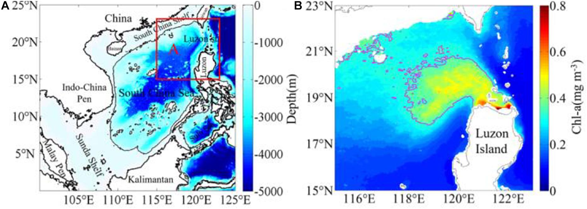
Figure 1. (A) Map of the South China Sea with the 200-m isobath; (B) the winter (December–February) mean chlorophyll-a (mg m^–3) concentration in the study region. The magenta contour, the Chl-a isoline of 0.35 mg m^–3, and the Chl-a data in the (B) is removed where the depth is shallower than 200 m; Box A (15–23°N, 115–123°E) in the (A), is the region of (B).

The upper SCS (i.e., the upper 200 m layer) is characterized by oligotrophic conditions and is nutrient (nitrogen/phosphate) limited (Wu et al., 2003) with strong light penetration all year round (Liu et al., 2002; Zhao and Tang, 2007). The mean SCS primary productivity is only about 350 mg m^–2 d^–1 (Liu et al., 2002). Nevertheless, higher Chl-a blooms are frequently observed in the vicinity of Luzon Strait in winter (Tang et al., 1999; Chen et al., 2006; Peñaflor et al., 2007; Wang et al., 2010; Shang et al., 2012) with the primary productivity of over 600 mg m^–2 d^–1 (Chen et al., 2006). This phenomenon of higher Chl-a bloom in winter was firstly reported by Tang et al. (1999) using remote sensing data. Also, Chen et al. (2006) confirmed the presence of phytoplankton blooms in the winter of 1999 using in situ data. And in-situ observations indicated also that the Nitrogen/Phosphate (N/P) ratio in winter is about 15 in the vicinity of Luzon Strait, very close to the Redfield value of 16. Since then, the prominent spatial and temporal characteristics and significances as well as the mechanisms of the phytoplankton blooms northwest of Luzon Island, have been investigated by many subsequent studies. Peñaflor et al. (2007) suggested the highest Chl-a concentration near the western slope of Luzon Strait to be related to the upwelling and the interaction of the northward Luzon coastal current with the intrusion of the Kuroshio during the northeast monsoon. Wang et al. (2010) emphasized that phytoplankton blooms are mainly regulated by the entrainment of the upper mixed layer by analyzing the seasonal variation of the phytoplankton southwest of Luzon Strait from 2000 to 2006. Using satellite remote sensing data from 1997 to 2007, Zhao et al. (2012) analyzed the spatial and inter-annual variations of phytoplankton blooms northwest of Luzon Island, and indicated that the Ekman pumping induced by the wind stress is the main factor causing high Chl-a concentration in winter. Shang et al. (2012) studied the phytoplankton blooms in January 2010, and their results suggested that phytoplankton blooms in the region near Luzon Strait were related to the mesoscale processes caused by the Kuroshio intrusion. Lu et al. (2015) developed a coupled physical-biological model to study the mechanisms of the winter bloom in Luzon Strait. The simulation for January 2010 showed that the nutrient supply was mainly caused by vertical mixing and subsurface upwelling while the advection of relative vorticity primarily contributed to the subsurface upwelling. Guo et al. (2017) proposed that the Kuroshio intrusion fronts enhanced chlorophyll concentration in the context of physical-biogeochemical interactions. To summarize, most of the aforementioned studies examined roles of wind stress curl, mixed-layer entrainment, coastal currents, and Kuroshio intrusion in individual winter blooms northwest of Luzon. Research is needed on interannual variability of the winter bloom in this region.

In this paper, we investigate the inter-annual variability and the spatial distribution of winter phytoplankton Chl-a blooms northwest of Luzon Island for the period from 1999 to 2015. We comprehensively consider the contribution of background environmental factors and examine the roles of various physical processes in the formation of winter phytoplankton bloom to provide an insight into the possible mechanism which drives the phytoplankton blooms.

Materials and Methods

Study Area

The study area lies in the northeastern SCS, approximately between 15°N to 23°N and from 115°E to 123°E (Figure 1B), where phytoplankton blooms occur frequently in winter (Tang et al., 1999; Chen et al., 2006; Peñaflor et al., 2007; Wang et al., 2010). In this area, the northeast monsoon first starts in September, covers the entire SCS in November, and peaks in December–January. The Kuroshio is a strong western boundary current of the North Pacific Ocean. The intrusions of the Kuroshio as a loop into the northeastern SCS and eddies shed from the Kuroshio into the SCS have been observed by previous studies (e.g., Shaw, 1991). The pattern of the intrusion circulation together with the wind stress curl and alongshore wind may be favorable for the occurrence of the upwelling in the region. As shown later in the paper, the higher Chl-a concentration is found mostly to begin in early November, lasting about 4 months. To investigate the complete process of the phytoplankton blooms from the bloom beginning, peak to slack-off, we consider 4 months (i.e., November, December, January, and February) as winter in the present study. To reduce the topographic influence of the shallow continental shelf on resuspension of sediments, including organic detritus and colored matter from the seafloor, as well as the influence of turbid Case-2 waters, the Chl-a data used in this study are limited to the open ocean with water depth deeper than 200 m.

Data

Chl-a data derived from SeaWiFS (Sea-Viewing Wide Field-of-View Sensor), MODIS (Moderate Resolution Imaging Spectroradiometer), MERIS (Medium Resolution Imaging Spectrometer), and VIIRS (Visible Infrared Imaging Radiometer) with the Garver-Siegel-Maritorena (GSM) Model (Maritorena and Siegel, 2005; Maritorena et al., 2010) are available from GlobColour database provided by HERMES. These data provide a large set of ocean color products with a time span ranging from 1997 to the present. The merged daily/monthly L3m Chl-a product, with a spatial resolution of 4 km, is utilized in this study for the period of 1999 – 2015.

Satellite-derived daily sea surface temperature (SST) data are obtained from the AVHRR (Advanced Very High Resolution Radiometer) in a spatial resolution of 0.25°. NOAA’s optimum interpolation sea surface temperature (OISST, also known as Reynolds’ SST) is also used in the present study. The OISST is a series of global analysis products from infrared satellite data spanning 1981 to the present.

The sea surface wind speed (WS) products are obtained from the QuikSCAT (Quick Scatterometer, 1999–2009) and ASCAT (Advanced Scatterometer, 2009–2015) provided by the Remote Sensing Systems in Santa Rosa, California with a spatial resolution of 0.25° × 0.25°. Both QuikSCAT and ASCAT wind fields are at 10 m above the sea surface.

Daily multi-mission merged Sea Level Anomalies (SLA) and Absolute Dynamic Topographies (ADT) both with 0.25° × 0.25° resolutions are available from the French Archiving, Validation, and Interpretation of Satellite Oceanographic data (AVISO) project. The dataset covers the period from 1993 to the present.

The World Ocean Atlas (WOA) is available from the Ocean Climate Laboratory of the National Oceanographic Data Center. World Ocean Atlas 2018 consists of a long-term set of climatology (annual, seasonal, and monthly) for temperature, salinity, oxygen, phosphate, silicate, and nitrate. There are 102 levels from the surface to 5500 m deep. The spatial resolution of seasonal temperature is 0.25°, and the spatial resolution of seasonal nutrient (phosphate, silicate, and nitrate) is 1°.

Expendable bathythermograph (XBT) data are the major component of the ocean temperature profile observations from the late 1960s through the early 2000s, and XBTs still continue to provide critical data to monitor surface and subsurface currents, meridional heat transport, and ocean heat content. The XBT profiles dataset corrected by Cheng et al. (2014) were used in our study, which can be obtained via the website¹.

In situ data during the period from the 27th to the 30th of January 2010 are also used in the study, which are from a transect survey that contained seven stations west of Luzon Strait, including Chl-a, temperature, and salinity profiles that are derived from the work of Shang et al. (2012) and Guo et al. (2017). The detailed data information can be found in Shang et al. (2012) and Guo et al. (2017).

Methods

The Sampling Region

In order to evaluate further the relationship between Chl-a and oceanic conditions, the time series of Chl-a and other oceanic parameters (i.e., WS, SLA, and SST) were produced for the three typical sub-domains in the study area. The following processes for choosing the Chl-a typical region are employed: first, the pixels with Chl-a pixel values greater than 0.35 mg m^–3 is selected for the value is roughly over two times of the mean annual Chl-a concentration; second, the center of the selected pixels is calculated according to the selected pixels; then, a “cell” is built that extends 1° eastward, northward, westward, and southward from the center respectively; at last, the average of the Chl-a values for all pixels is calculated within the cell. WS and SLA are processed into time series by a similar approach as Chl-a by using the threshold of 8 m s^–1 and 0.01 m. Considering that the maximum of Ekman transport (ET) and Ekman pumping velocity (EPV) occur offshore, we selected the two fixed cells located in 118.5–120.5°E, 18–20°N for ET and in 118–120°E, 16.5–18.5°N for EPV, where the variations of ET and EPV are more notable respectively. The time series of SST is also produced for the fixed cell located in 118.5–120.5°E, 18–20°N.

There are only 1–3 suites of XBT data in winter from 1999 to 2009. The XBT data in the study area are averaged if there are two suites or more for a winter. The averaged values are used to represent the XBT profile for that winter. The data after processing will be utilized to analyze the inter-annual variation of the temperature profiles.

Ekman Transport and Ekman Pumping Velocity

Ekman transport and Ekman pumping velocity are calculated with the wind stress vector $\overrightarrow{\tau }$, and the calculation formula of ET is:$\overline{M}=\frac{1}{\mathrm{\rho }f}\overrightarrow{\tau }\times \stackrel{\mathrm{\wedge }}{\mathit{t}}$, Ekman pumping velocity (EPV) is:EPV=-curl$\left(\frac{\stackrel{-}{\tau }}{\mathrm{\rho }f}\right)$, where ρ is sea water density (1.025 × 10³kg m^–3), f is Coriolis parameter (f = 2ωsin⁡φ),t∧ is a unit vector tangent to the local coastline. The wind stress is calculated as follows:τ = C_Dρ_a⋅u², where ρ_a is the air density close to the sea surface (here,ρ_a = 1.29kgm⁻³), u is wind speed, C_D is the drag coefficient and it is a function of wind speed, sea air temperature difference, and sea condition. In order to weigh the relative influence of ET and EPV, the vertical/upwelling speed derived from the offshore ET is further calculated by$ETV=\frac{M}{R_0}$, where R₀ is first baroclinic Rossby radius, and the value of R₀ is about 50 km northwest of Luzon Island (Cai et al., 2008).

EOF Analysis

The method of empirical orthogonal function (EOF) analysis (Bjornsson and Venegas, 1997) is a decomposition of a signal or data set in terms of orthogonal basis functions which are determined from the data. It is similar to performing a principal component analysis of the data, except that the EOF method finds both time series and spatial patterns. The essence of the EOF analysis is to identify and extract the spatial-temporal modes that are ordered in terms of their representations of data variance. It decomposes the data matrix of the original variable field into the eigenvector matrix (spatial function) and the time coefficient matrix (time function), which is suitable for extracting the main data characteristics of the elements. Each of these orthogonal functions is ranked by its temporal variance (Xu et al., 2011). The typical distribution structure of the variable field is expressed by the first few unrelated feature vectors, the time coefficient corresponding to the eigenvector represents the time variation characteristic of the different distribution form. The positive value indicates that the variable field is decomposed at this time and the spatial distribution of the eigenvector as present showed, while the negative value is the opposite. And the larger the absolute value of the time coefficient, the more typical the distribution pattern is, the closer the coefficient is to the zero, the distribution of the form is less significant.

The Multiple Correlation Analysis

The multiple correlation analysis is a statistical technique that predicts values of one variable on the basis of two or more other variables. The closer the multiple correlation coefficient is to 1, the stronger the linear relationship between the dependent and causative variables. The partial correlation method is used to describe the relationship between two variables, while the effect of all other variables is removed from this relationship. It allows us to determine the correlation between any two variables (hypothetically), if all other variables are held constant. The coefficient of multiple correlation can be computed as follows: $R_{y\cdot 12\mathrm{\cdots }m}=\sqrt{1-\frac{|R|}{R_{yy}}}$, and the partial correlation coefficients between x_i and y are given by: $R_{yi\cdot 1,2,\mathrm{\cdots },m}=\frac{R_{yi}}{\sqrt{R_{yy}{R}_{ii}}}$. Here, y is the dependent variable and x₁,x₂,…,x_m is the causative variables, R is the correlation matrix between variables x₁, x₂, …, x_m, y: $R=\begin{array}{ccccc}{r}_{11}& r_{12}& \cdots & r_{1m}& r_{1y}\\ r_{21}& r_{22}& & r_{2m}& r_{2y}\\ & ⋮& \ddots & ⋮& \\ r_{m1}& r_{m2}& \dots & r_{mm}& r_{my}\\ r_{y1}& r_{y2}& & r_{ym}& r_{yy}\end{array}$; Here r_ij is the simple correlation coefficient between x_i and x_j. r_iy and r_yj are the simple correlation coefficient between x_i and y and between y and x_j, respectively. Moreover, r_ii=1, r_ij = r_ji, and r_iy = r_yt. | R| is the determinant of the matrix R; R_yy is the algebraic cofactor of the matrix after removing the m + 1 row and the m + 1 column in |R|;R_yy, R_ii and R_yi are the algebraic cofactors of r_yy, r_ii, and r_yt in |R|, respectively (Zhao and Wang, 2018).

Stepwise Regression

Stepwise regression (Jennrich, 1977) is a systematic method for adding and removing terms from a multi-linear model based on their statistical significance in a regression. The method begins with an initial model and then compares the explanatory power of incrementally larger and smaller models. At each step, the p-value of an F-statistic is computed to test models with and without a potential term. If a term is not currently in the model, the null hypothesis is that the term would have a zero coefficient if added to the model. If there is sufficient evidence to reject the null hypothesis, the term is added to the model. Conversely, if a term is currently in the model, the null hypothesis is that the term has a zero coefficient. If there is insufficient evidence to reject the null hypothesis, the term is removed from the model.

The stepwise regression selects variables in a step-by-step manner. The procedure adds or removes independent variables one at a time using the variable’s statistical significance. It either adds the most significant variable or removes the least significant variable.

Results

Distribution of Chl-a Concentration Northwest of Luzon Island

The monthly mean Chl-a concentration averaged for 16 years shows the general seasonal cycle of Chl-a distribution northwest of Luzon Island during the period 1999–2014 (Figure 2). The Chl-a in coastal waters is generally higher than that in offshore waters. The Chl-a in winter is the highest among the four seasons. The lowest Chl-a concentration is observed west of Luzon Island (south of 19°N) in summer and east of Luzon Strait almost all year round. The highest Chl-a concentration is only observed near the northern SCS shelf in summer. However, the patch of relatively high Chl-a concentration exists in the offshore waters northwest of Luzon Island during the northeastern monsoon, which can’t be observed in the other seasons. The high Chl-a concentration patch occurs first in November (i.e., the initiation period), peaks in December or January (i.e., the peak period), and then decays in February (i.e., the decay period).

FIGURE 2

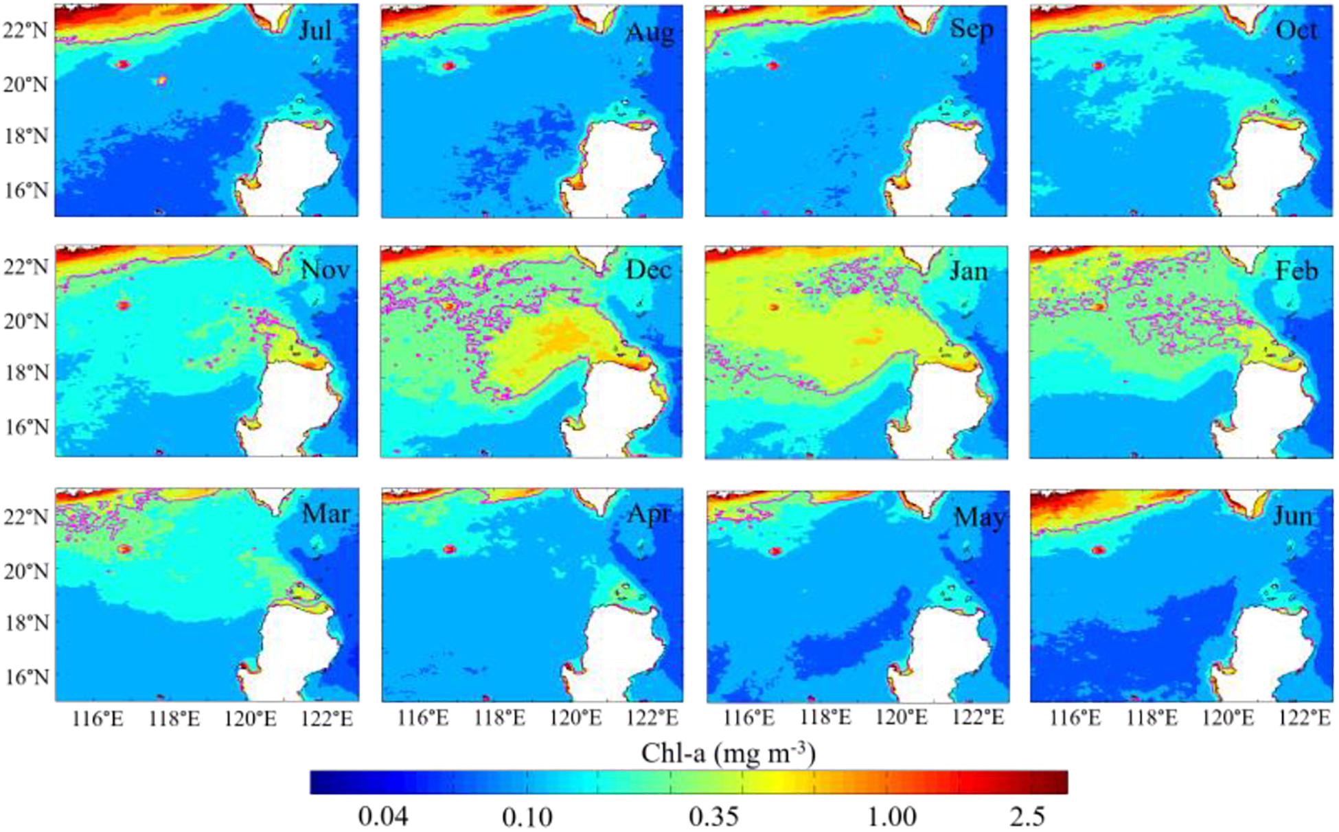
Figure 2. Monthly mean merged Chl-a concentration with a spatial resolution of 4 km in the period 1999–2015. Magenta contours depict the Chl-a concentration is 0.35 mg m^–3.

The first EOF mode also shows the typical spatial and temporal distribution of Chl-a northwest of Luzon Island. There are high weighted-values (Figure 3A) northwest of Luzon Island. Combined with the first EOF mode, the first principal component (with the contribution of 38.23% to the total variability of Chl-a) indicates that the highest Chl-a concentrations are presented in winter, suggesting that the blooms prevail frequently in winter. The spatial patterns show a strong positive signal of Chl-a concentrations over a 2° by 2° area centered at about (119.5°E, 19.5°N). The seasonal variability is reflected by the time-series of amplitude coefficient (Figure 3B) associated with the spatial pattern of the first mode (Figure 3A). The relatively high temporal amplitude coefficient of the first mode (Figure 3B) occurs 12 times in January and four times in December. In addition, the highest amplitude occurs in January of 2015, followed by December of 2003, January of 2012, January of 2014, and so on.

FIGURE 3

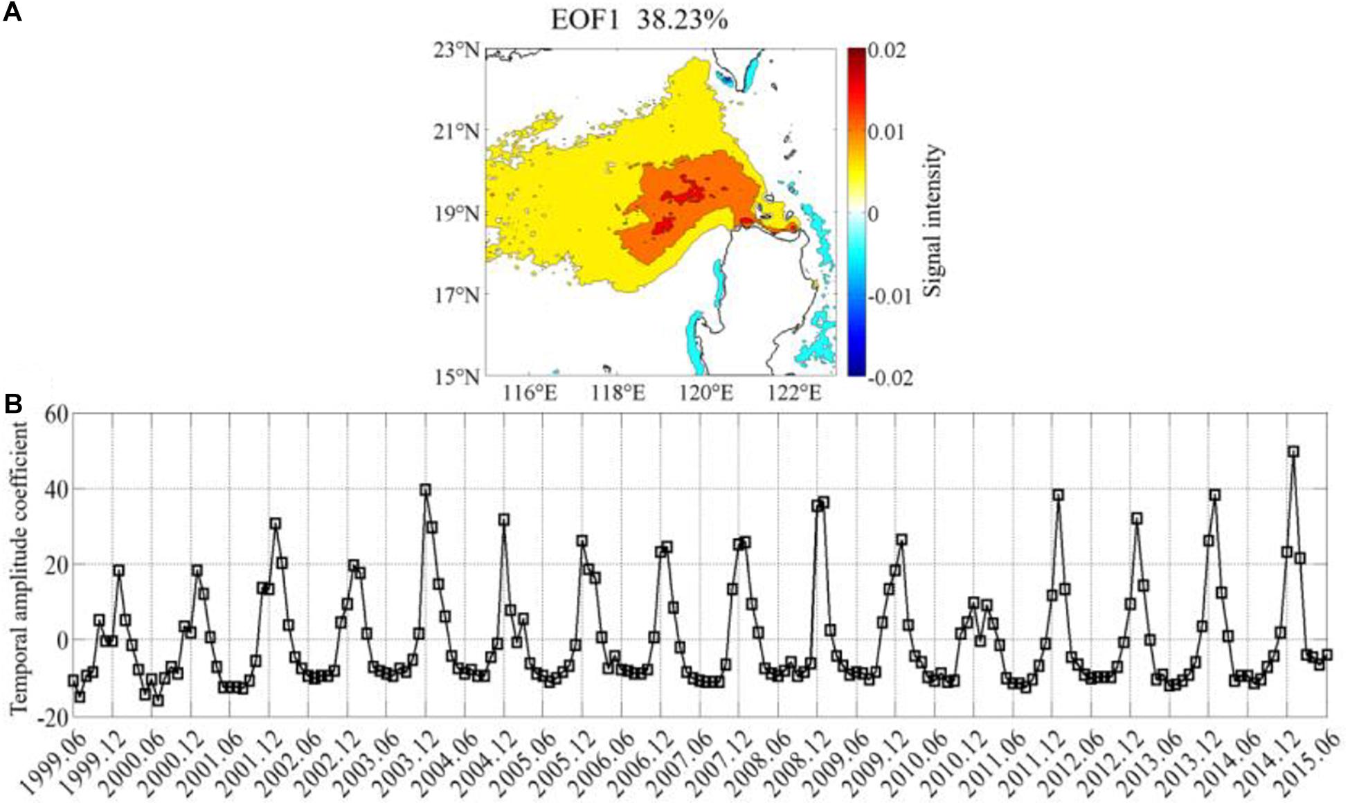
Figure 3. The first EOF mode of the chlorophyll-a concentration in the study area: (A) spatial pattern of the first EOF mode, the percentage of variance explained is 38.23%; (B) time series of the amplitude of the first EOF mode (The Chl-a data in EOF analysis is investigated in the offshore region with water depth over 200 m).

According to the winter time-series of averaged Chl-a in the 2° × 2° cell from 1999 to 2014 (Figure 4), Chl-a concentration is found considerably higher in December or January than in November and February. Higher Chl-a concentration is seen in the winters of 2003, 2007, 2013, and 2014, but a minimum is presented in the winter of 2010. Also, there is no significant intra-seasonal variation of Chl-a distribution in the winter (i.e., November–February) of 2007. The winter (November–February) Chl-a concentration in 2001, 2003, 2005, 2007, 2009, 2013, and 2014 exceeds the winter Chl-a climatology over 1999–2014. At the same time, the total Chl-a concentrations in these winters are higher than in other winters. Furthermore, the variation of this time series is qualitatively similar to the temporal amplitude coefficient of the first mode (Figure 3B), with the highest Chl-a concentration in the 2014 winter and the lowest in the 2010 winter.

FIGURE 4

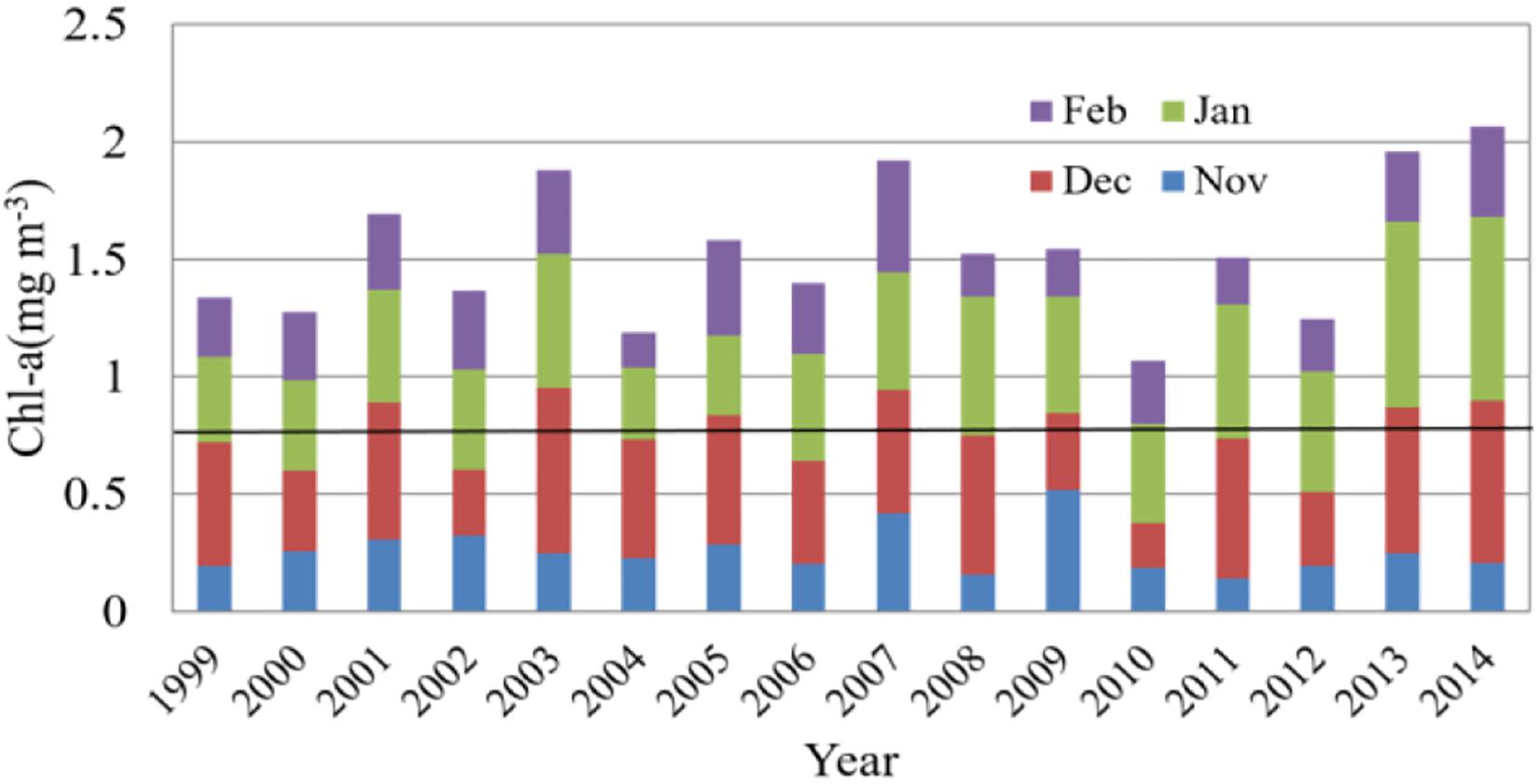
Figure 4. Time-series of the winter Chl-a concentration in the 2° × 2° cell from 1999 to 2014. The bold black line in figure represents half of the cumulative Chl-a concentration averaged for winter of 1999–2014.

Satellite Observation of Environmental Conditions

Wind-Induced ET and EPV

The wind stirring in the upper ocean, wind-induced Ekman transport (ET) and Ekman pumping can bring nutrient-rich deeper water into the surface layer, which may exert important effects on the distribution of Chl-a. In our study area, during the prevailing northeast monsoon, the mean sea surface wind speed reaches 8 m s^–1 or more, and the wind speed is over 10 m s^–1 west of Luzon Strait. Winds could trigger coastal upwelling by wind-induced offshore Ekman transport. Ekman transport northwest of Luzon Island is the strongest in December, the weakest in February, and comparable in November and January (Figure 5A). The strong ET is roughly located in (118.5–120.5°E, 17.5–20.5°N) northwest of Luzon Island (Figure 5A). Wind also can regulate Ekman pumping. Significant Ekman pumping caused by the wind stress curl is located about at 118–120°E, 16–19°N (Figure 5B), and the variation of EPV is roughly consistent with that of ET. Both higher ET and EPV occur in the nearshore region west of Luzon Island. Wind-induced offshore ET reaches about 4 m² s^–1, which can induce the upwelling speed of about 8 × 10^–5 m s^–1 in the coastal waters, while the upwelling caused by EPV of ∼1.5 × 10^–5 m s^–1, the upwelling in the coastal waters by ET is over five times of the mean EPV. Also, higher ET extends westward (perpendicular to the coast) while higher EPV extends southwestward.

FIGURE 5

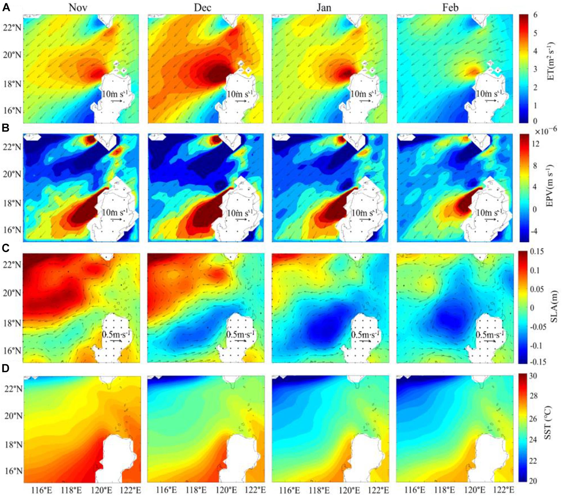
Figure 5. Monthly mean (A) Ekman Transport (ET), and (B) Ekman Pumping velocity (EPV) derived from Sea surface wind speed (WS) products of the QuikSCAT and ASCAT, (C) Sea Level Anomalies (SLA) from AVISO, (D) Sea Surface Temperature (SST) from AVHRR with a spatial resolution of 0.25° in winter. The arrows in (A,B) indicate the direction and size of wind speed. The arrows in (C) indicates the direction and size of the geostrophic flow.

SLA and Geostrophic Flow

There exists a relatively lower SLA (Figure 5C) northwest of Luzon Island during winter. The lower SLA is approximately located in 116.5–120.5°E, 16.5–19°N (Figure 5C). The low SLA center is spatially variable, approximately at 117.5°E, 17°N during November, 118.5°E, 17.5°N during December and 119°E, 18°N during January, while in February it lies farther northward than in other 3 months. The sea surface height in the upwelling region is usually lower than that in the surrounding area. The region of low SLA centers suggests the existence of upwelling. The direction of the geostrophic currents is roughly aligned with the direction of the higher Chl-a center moving. These phenomena imply that the center of the Chl-a bloom might be affected by the ocean currents (i.e., the advection effect).

Temperature Distribution

The study area is located in the tropical–subtropical ocean, so the annual mean SST is relatively high. Since strong northeast monsoon can result in severe sea surface heat loss in winter, the average winter SST in the study area is 25.29°C. The SST shows lower temperature northwest of Luzon Strait, which extends toward the southwest (Figure 5D). The temperature range of 20–25°C is generally suitable for phytoplankton growth (Eppley, 1972; G-Yull and Gotham, 1981; Grimaud et al., 2017). Thus, the temperature of the study area is more suitable for phytoplankton growth in winter, compared with higher SST in other seasons.

In situ Observations Northwest of Luzon Island

Climatological Temperature and Nutrients Distribution From WOA

The distribution of the WOA climatology temperature (Figure 6A) in the upper ∼25 m layer in winter is consistent roughly with that of satellite observational SST (Figure 5D). However, the WOA climatology temperature (Figure 6A) in the 50–100 m layer northwest of Luzon Island displays an evident cold-water patch of 117.5–120.5°E, 16.5–19.5°N. The patch of the low temperature below the 50-m layer presented in the climatology WOA temperature data (Figure 6A) also confirms the existence of upwelling in the region. Besides, with the increase of depth (from the depth of 50 m to the depth of 100 m), the cold-water center shifts slightly northward.

FIGURE 6

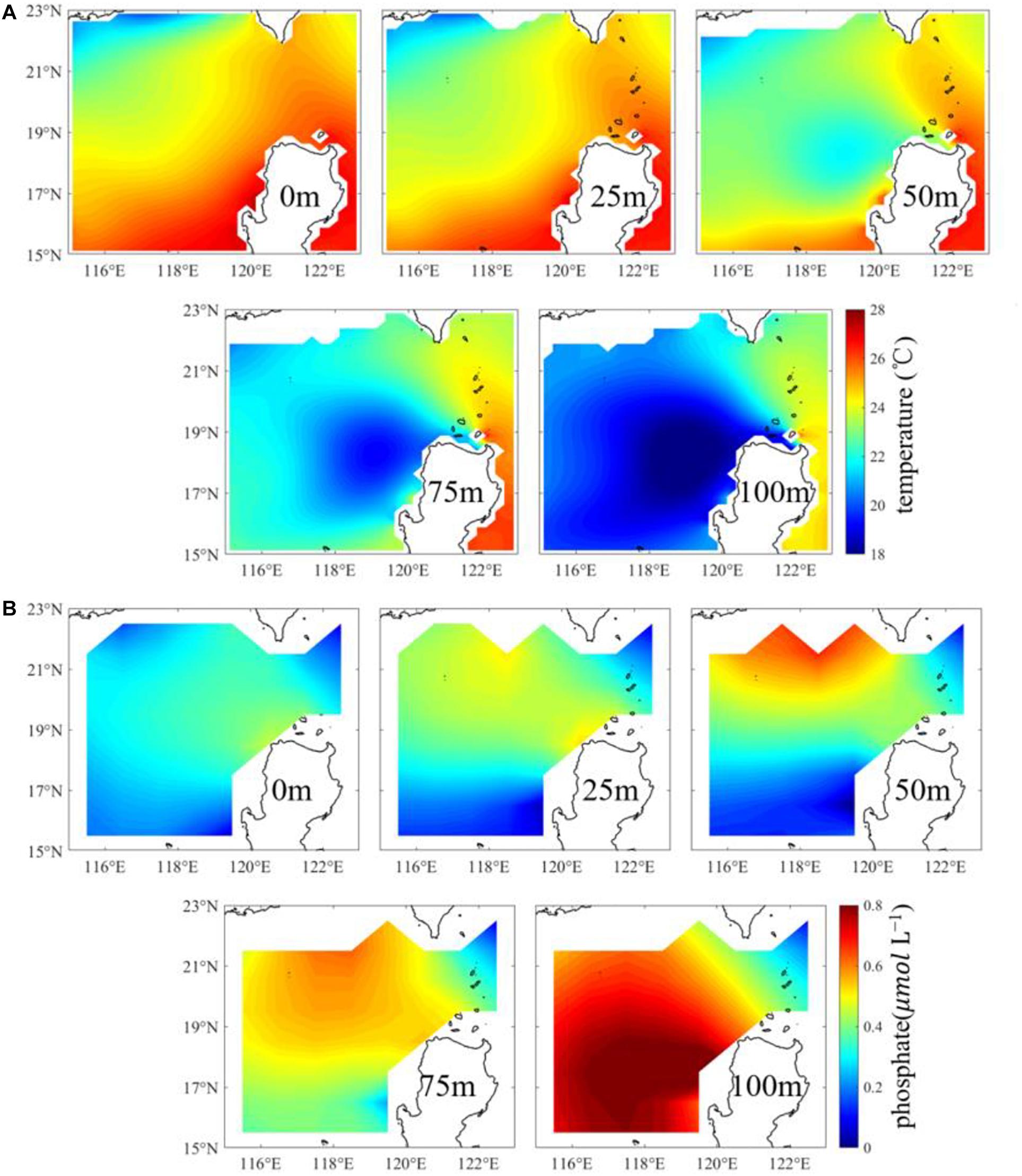
Figure 6. The winter seasonal climatology of (A) temperature and (B) phosphate at depths of 0, 25, 50, 75, and 100 m from WOA18 with a spatial resolution of 0.25° and 1° respectively.

In the upper oligotrophic tropical oceans like the SCS with abundant sunlight, the maximum euphotic layer depth can reach 110 m with evident seasonal changes (Shang et al., 2011; Zhao and Wang, 2018). Nutrients are generally low in the upper euphotic layer because of consumption by phytoplankton photosynthesis and barrier of nutrients injection into the upper layer by the pycnocline (Ledwell et al., 1993). Phosphate content ranges from 0 to 0.8 μmol L^–1 (Figure 6B). There exists a high phosphate center (116–120°E, 16–19.5°N) at the depth of 100 m northwest of Luzon Island. This high concentration distribution of phosphate at the 100 m depth is matched with the low temperature center at the corresponding depth. However, the high phosphate concentration shifts further north at the depth shallower than 75 m.

Interannual Variation of Temperature From XBT in Winter

Here, we select a set of XBT sections northwest of Luzon Islands (located in 118–121°E, 18–21°N) in winter from 1999 to 2009 as a proxy of the vertical water temperature every year (Figure 7). The phytoplankton growth is deeply influenced by temperature, due to the temperature is an important factor affecting the stability of the upper ocean. The XBT profiles in the upper 50 m indicate the high mean temperature in 1999 and 2002 and low mean temperature in 2007. Table 1 presents the temperature difference between the sea surface and the 50 m depth and the depths where the temperature decreases by 0.5 °C from the surface temperature for each year. Combined with the temperature profile of the upper 100 m, it can be found that the difference of temperature between the sea surface and the 50-m depth is relatively smaller and the depth where the temperature is 0.5°C lower from the sea surface is relatively larger in 2001, 2003, 2008, and 2009 (Figure 7 and Table 1).

FIGURE 7

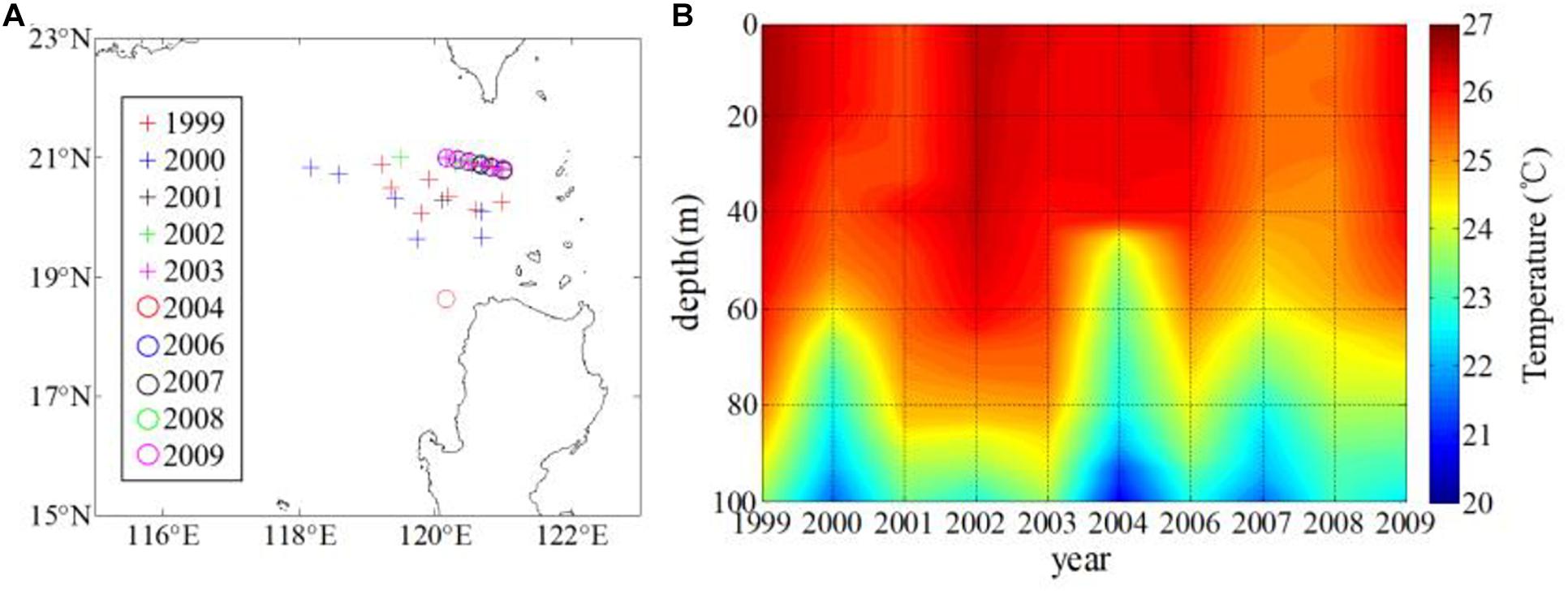
Figure 7. (A) Location of selected XBT set and (B) profile of temperature in the upper 100 m in winter.

TABLE 1

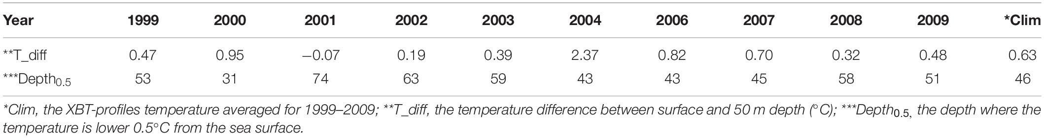
Table 1. Temperature difference between the surface and the 50 m depth and the depth where the surface temperature is 0.5°C colder than the surface.

Ship-Based Observations West of Luzon Strait During 27–30 January 2010

The ship-based observations are used in our study. The near surface (the 5-m layer) Chl-a concentrations at all sites (Figure 8B) are similar to the surface Chl-a concentrations observed by satellite (the background shading in Figure 8A), with a high correlation coefficient (Figure 9) between them (r = 0.86, p < 0.05). From north to south, the near surface Chl-a is relatively high at sites of E402, E403, E404, and E405 (>0.4 mg m^–3). According to the vertical profiles of Chl-a (Figure 8B), the maximum Chl-a concentration appears in the subsurface layer instead of the surface layer except station E403. Although the near surface layer Chl-a concentration is lower at the station E406, its Chl-a concentration in the 50-m layer is higher than that at most other stations. Contours of temperature (Figure 8C), salinity (Figure 8D) and density (Figure 8E) elevated upwards around 19°N, which indicates the existence of upwelling and mixing.

FIGURE 8

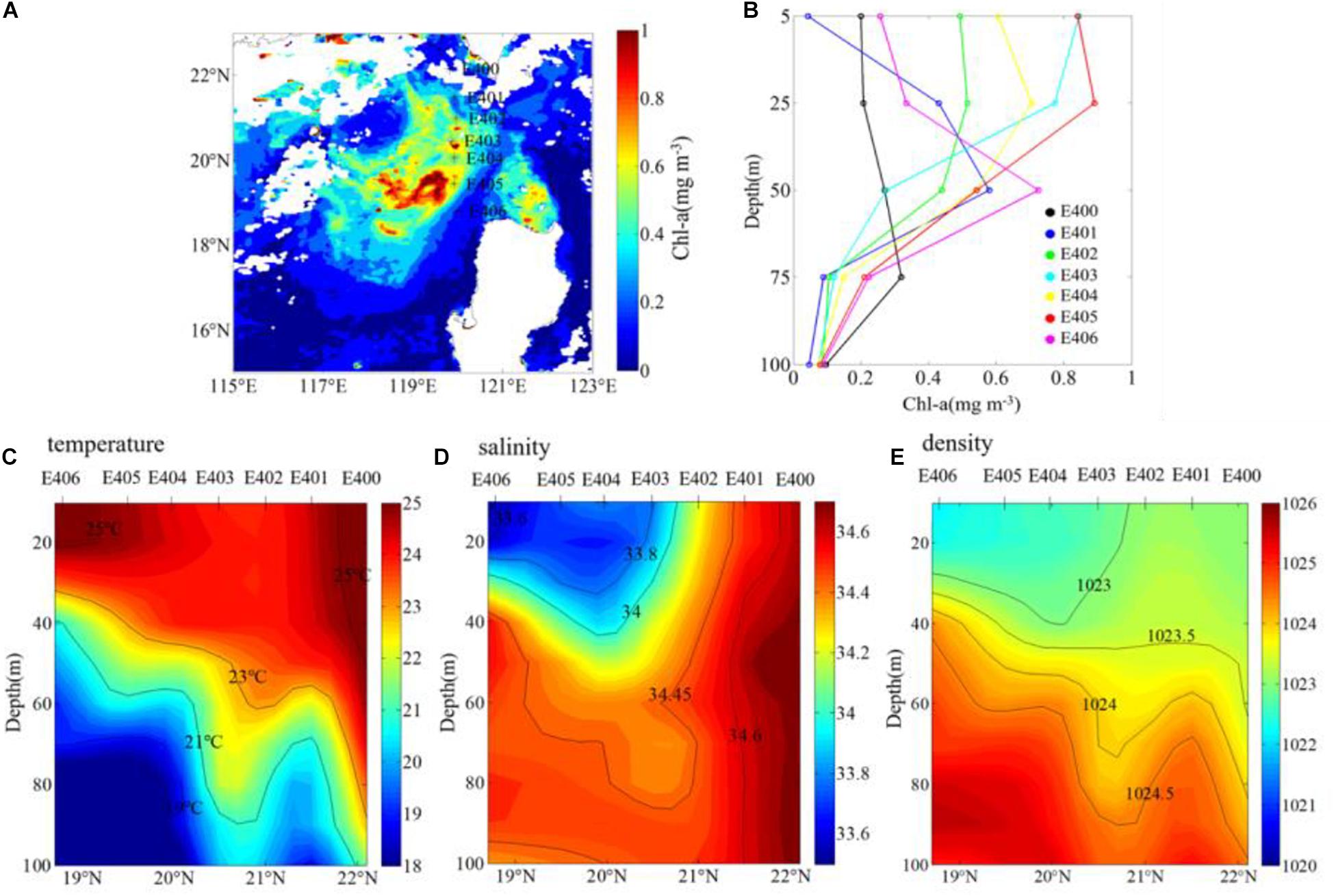
Figure 8. In situ observations during 27–30 January 2010: (A) the location of Stations E400–E406, the background shading denotes surface mean Chl-a during 27–30 January 2010 which obtained from GlobColour (daily data) (B) vertical profiles of Chl-a (mg m^–3). Cross-section diagram of (C) temperature (°C), (D) salinity (psu), and (E) density (kg m^–3) along the E transect.

FIGURE 9

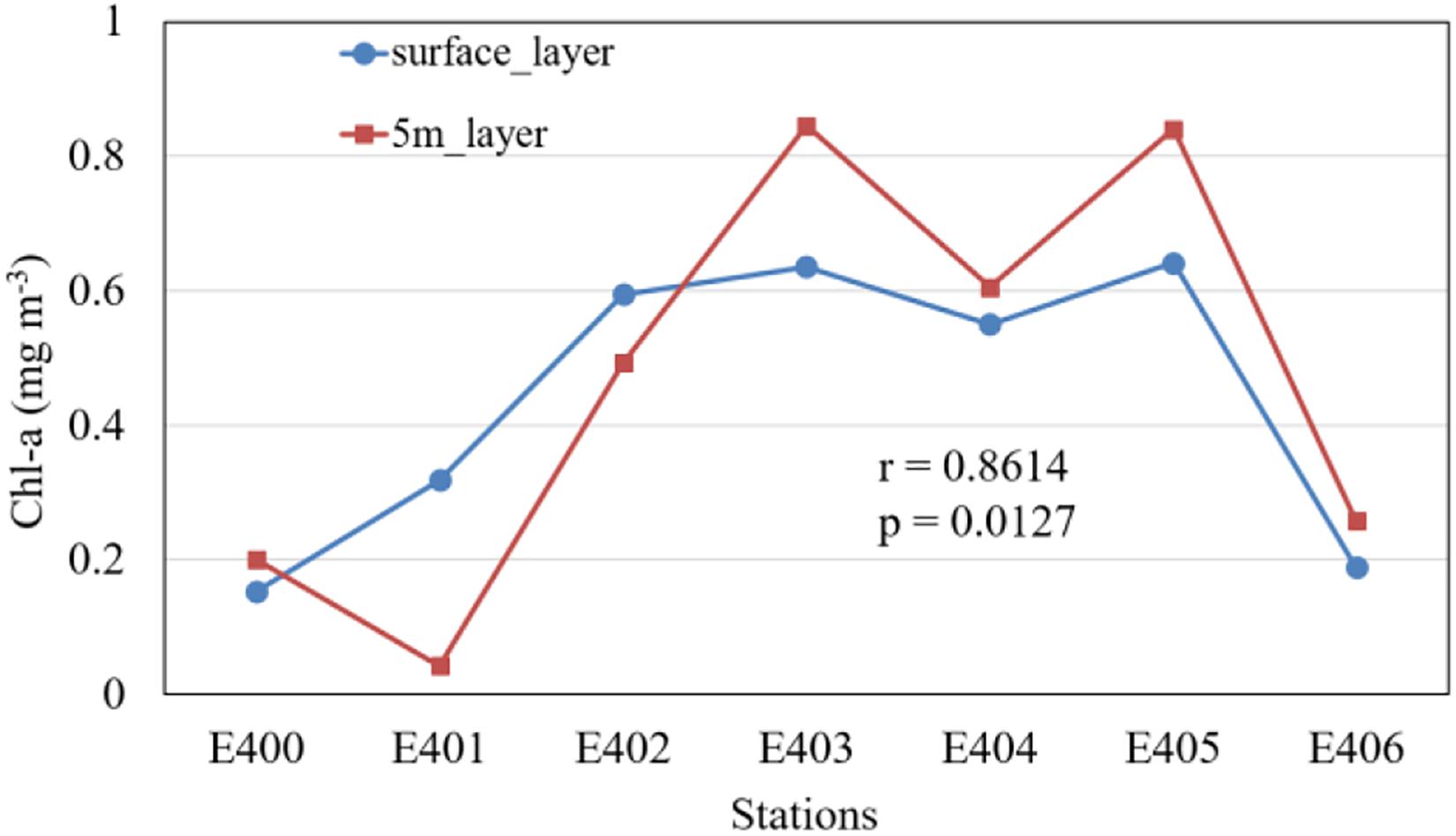
Figure 9. Comparison of chlorophyll concentration at each station derived from satellites (i.e., surface layer) and in situ observation (i.e., 5 m-layer). The surface-layer Chl-a is produced through averaging Chl-a values for 2 pixels by 2 pixels near the in-situ stations, based the Chl-a data averaged for daily GlobColour data of 27–30 January 2010.

Time Series of Chl-a and EPV, ET, WS, SLA, SST in Winter

Simple correlation analysis indicates that Chl-a (Table 2) is positively correlated with EPV, ET, and WS, and negatively correlated with SLA and SST (Chl-a vs. EPV, r = 0.37, p < 0.01; Chl-a vs. ET, r = 0.52, p < 0.01; Chl-a vs. WS, r = 0.48, p < 0.01). The pattern of Chl-a variation is similar to that of EPV, ET, and WS (Figure 10), usually with higher wind speed, EPV, or ET accompanied by higher Chl-a. Chl-a also shows a good correlation with SLA and SST (Chl-a vs. SLA, r = −0.37, p < 0.01; Chl-a vs. SST, r = −0.48, p < 0.01). The above results indicate the covariant characteristics of Chl-a concentration and marine environmental conditions.

TABLE 2

Table 2. The simple correlation coefficients between Chl-a blooms and ocean conditions.

FIGURE 10

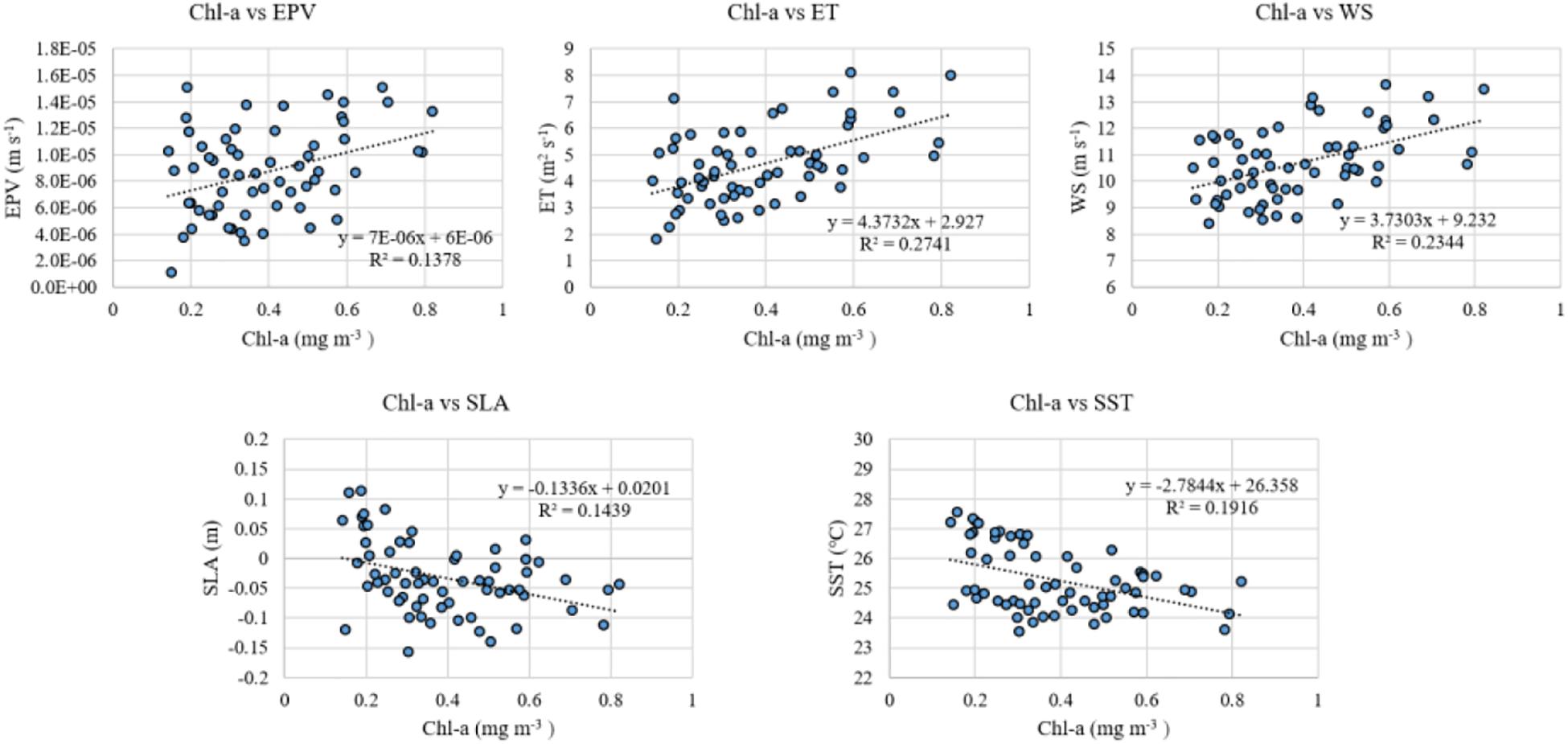
Figure 10. Scatter diagrams of monthly Chl-a, EPV, ET, WS, SLA, and SST in winter averaged for the selected regions, respectively. The boxes used in time series of Chl-a, EPV, ET, SLA, and SST are chosen according to the rule mentioned in Section “The Sampling Region.”

The multiple correlation analysis indicates that the coefficient of multiple correlation (Table 3) between Chl-a and environmental factors (i.e., EPV, ET, WS, SLA, and SST) is significant (R = 0.785, p < 0.01). The partial coefficients of Chl-a concentration with EPV, ET, SLA, and SST are −0.061, 0.255, 0.205, −0.123, and −0.362, respectively (Table 3), indicating that ET and SST played important roles in the winter blooms.

TABLE 3

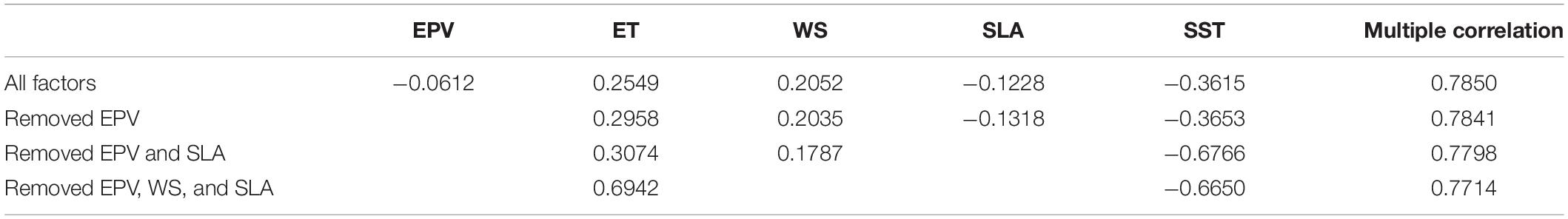
Table 3. The multiple correlation and partial coefficients between the Chl-a and other oceanic factors.

Using a Stepwise Multiple Linear Regression (Table 4), we verify the relationship between Chl-a and oceanic factors (WS, EPV, ET, SLA, and SST), and examine the relative importance of the five factors (Table 4). Chl-a is chosen as the dependent variable, and WS, EPV, ET, SLA, and SST the independent variables in the stepwise multiple linear regression to determine their relationship. ET is first included due to its smallest p-value, which indicates that the ET is important in the variation of Chl-a. The SST is then added into the regression equation, better correlation coefficient between ET, SST and Chl-a is obtained. Subsequently, there are no terms which could be added. Thus, the regression equation has two variables (i.e., ET and SST), which suggests the significant importance of ET and SST played in the variation of Ch-a.

TABLE 4

Table 4. Correlation coefficient using a stepwise multiple linear regression, significance level, F-statistic, RMSE and regression equation.

Discussion

Marine phytoplankton productivity is usually limited by nutrient supply and light intensity (Tang et al., 2004; Siegel et al., 2007). Our study area is located in a tropical-subtropical ocean with light intensity adequate for phytoplankton photosynthesis in the upper layer (Liu et al., 2002; Chen et al., 2006; Peñaflor et al., 2007; Zhao and Tang, 2007). The phytoplankton growth in the upper layer of the study area may be mainly regulated by nutrients availability. Therefore, the key to better understand the dynamical mechanism of winter phytoplankton blooms in the study area is to investigate the physical processes of the upper sea associated with the supply of nutrients. We focus on the physical processes of the upper ocean affecting the supply of nutrients in the present study. The complex marine physical processes in this area mainly include the upwelling induced by wind stress, and the horizontal/vertical movement of the water column caused by the ocean currents, all of which require further investigation.

Influence of Environmental Elements on the Winter Phytoplankton Blooms

A good consistency (r = 0.86, p < 0.05) of the surface Chl-a concentrations (Figure 9) is found between the in situ observations and the satellite remote sensing observations, suggesting that the satellite ocean color data used in the study region are reliable in the study region to a certain degree. In our study, the winter phytoplankton bloom (Figure 2) occurs firstly in November, peaks in December or January, and decays in February. The ET, EPV, WS, and SLA also show monthly changes during November – February (Figure 5). The Chl-a presents a high correlation with various environmental conditions (EPV, ET, WS, SST, and SLA) based on the simple correlation analysis (Table 2). The multiple correlation coefficient (Table 3) between Chl-a and these environmental factors including EPV, ET, WS, SST, and SLA (r = 0.785, p < 0.01) also indicates further that all these environmental factors exert important impacts on the winter Chl-a bloom northwest of Luzon Island.

According to the analysis of multiple and partial correlations (Table 3), we find that ET and SST have more significant effects on the Chl-a bloom. Though Ekman pumping also shows a good simple correlation coefficient with Chl-a (r = 0.37, p < 0.01), there exists an insignificant partial correlation (r = −0.0612) between Chl-a and EPV, suggesting less influence of EPV on surface Chl-a. After removing EPV, we find that the multiple correlation coefficient has only a slight drop, also indicating a weak impact of EPV on Chl-a. This finding is obviously different from previous studies (Chen et al., 2006; Shang et al., 2012; Zhao et al., 2012) that Ekman pumping was thought to play an important role in the winter phytoplankton bloom, which however, focus on individual cases of winter blooms only. After EPV, SLA, and WS are removed from the multiple correlation analysis, the winter Chl-a bloom still shows a significant correlation (multiple correlation coefficient, R = 0.7714, p < 0.01) with ET and SST along with partial correlation coefficients of 0.6942 and −0.6650, respectively. Besides, the analysis obtained by the multivariate stepwise linear regression also indicates that the two remaining items (i.e., ET and SST) cannot be removed, implying that the variations of ET and SST are of essential importance in the winter Chl-a bloom.

Significant variation of ET is more consistent with that of Chl-a when compared with those of EPV, SLA and vorticity derived from geostrophic currents, as indicated by the partial coefficients. ET-induced upwelling, which accounts for the total upwelling more than Ekman pumping-induced upwelling (∼8 × 10^–5 m s^–1 for ET vs. ∼1.5 × 10^–5 m s^–1 for EPV), can provide a continuous source of cold, nutrient-rich water to the surface euphotic zone, replacing the nutrient-depleted water (Chereskin and Price, 2001). Moreover, the strong ET area is much closer to the high Chl-a location than the strong EPV area. According to the distribution of temperature (Figure 6A) and nutrients (i.e., phosphate in Figure 6B), the locations of lower temperature and higher phosphate concentrations in the upper 75–100 m layers are roughly the same, which coincide with the location of the ET-induced upwelling region. The phenomenon suggests the existence of ET-induced upwelling, which may cause the high Chl-a concentration at the sea surface.

The pattern of temperature (e.g., SST) is usually taken as an important indicator for not only upwelling, but also mixing intensity (Tang et al., 2002). Lower SST would enhance the instability of the upper-layer water column, favorable for vertical mixing (Phillips, 1966), increasing nutrients in the euphotic layer. Therefore, the lower SST reflects a higher probability of available nutrients into the euphotic zone, showing the higher correlation between the Chl-a and the SST (Figure 8E and Table 2). A high temperature gradient reflects upwelling tendency as well as stable stratification. There is higher instability of the upper ocean in 2001, 2003, 2008, and 2009 (Figure 7 and Table 1), when Chl-a concentrations are relatively high (Figure 4). On the contrary, stratification northwest of Luzon is stronger in 2000, 2004, and 2006. The increase in the instability of stratification is favorable to the nutrient-rich water being mixed into the shallower layer, and vice versa. Thus, the vertical movement in the upper ocean is stronger (weaker) in the years of 2001, 2003, 2008, and 2009 with the stronger winter Chl-a blooms (in the years of 2000, 2004, and 2006 with the weaker winter Chl-a blooms) (Table 1 and Figure 4). Therefore, the instability of stratification associated with the vertical temperature difference is probably the reason that SST presented a better correlation with the winter Chl-a bloom.

Role of the Northward Flow in the Dislocation of the Phytoplankton Bloom and Wind-Induced Upwelling Centers

The existence of upwelling and the phenomenon of phytoplankton blooms northwest of Luzon in winter have been reported in different ways as mentioned above. Our results from multiple correlation analyses also indicated that upwelling is the principal reason for the winter blooms, but our conclusions are somewhat different.

Generally, upwelling regions are usually of high biological productivity (McGillicuddy et al., 2007; Etourneau et al., 2009; Ganachaud et al., 2010; Tremblay et al., 2011; García-Reyes et al., 2014). Upwelling is usually calculated by Ekman pumping velocity or Ekman transport. Ekman pumping and Ekman transport in our study area are strong (Figures 5A,B) during winter, suggesting the existence of the prevailing upwelling northwest of Luzon Island. And this region is famous for the Luzon cold eddy, divergence in cold eddy also contribute to the upwelling. According to the temperature distribution below the 50-m depth (Figure 6A) and nutrients with depth (Figure 6B) below the 75-m depth from WOA18, there is an evident center of low temperature southwest of Luzon Island (50 – 100 m layers in Figure 6A), which is especially closer to the center of ET, suggesting also the existence of upwelling. Moreover, the cross-section diagrams of temperature (Figure 8C) and density (Figure 8E) along the E transect indicate also the existence of the evident upwelling and mixing around 19°N in the 2010 winter. Therefore, winter upwelling plays an important role in the formation of phytoplankton bloom in the region.

The center of upwelling induced by EPV (∼119.5°E, 17.5°N, Figure 5B), the center of low SLA (116.5–120.5°E, 16.5–19°N, Figure 5C) and the center of low temperature below 50 m layers (∼119°E, 18°N in Figure 6A) are inconsistent with the surface high Chl-a concentration center (∼119.5°E, 19.5°N, Figures 1B, 2). Although the center of ET (∼120°E, 18.5°N) is closer to the center of Chl-a, the two centers are not the same. There exists a strong northward coastal current west of Luzon (NCCWL) in winter (Chao et al., 1996; Shaw et al., 1996). The NCCWL region (Figure 11) is in a region approximately from 16 to 19.5°N and from 119 to 121°E. The northward geostrophic flow velocity calculated by the Absolute Dynamic Topography (ADT) northwest of Luzon is about 0.13 m s^–1 in winter. Thus, the water mass in the upwelling area can be transported northward about 160 km in 2 weeks. The northward movement of NCCWL may exert a certain effect on the difference between the locations of phytoplankton blooms and wind-induced upwelling. The upwelling around 16–19°N (i.e., EPV, SLA, the temperature below 50 m and ET) bringing nutrient-rich deeper water into subsurface (high phosphate concentration at 100 m), and is carried by northward flow to the surface layer. Also, according to the vertical profiles of Chl-a (Figure 8B), the station E406 shows relatively low Chl-a concentration at the surface, but it shows higher concentration at the depth of 25 and 50 m, which may imply the northward movement. Moreover, ET-induced upwelling near the coastal northwest Luzon Island is located on the southeast side of the high Chl-a center, the northward geostrophic flow ends around 19.5°N, then move to the west (Figure 11), affecting nutrients and phytoplankton near ET-induced upwelling move to the northwest. The westward geostrophic flow velocity northwest of Luzon Island is also relatively strong, which is consistent with the Chl-a distribution. The oceanic temperature in the nearshore region northwest of Luzon (Figures 5D, 6A) is higher than elsewhere in the same latitude, which also affirms the existence of NCCWL.

FIGURE 11

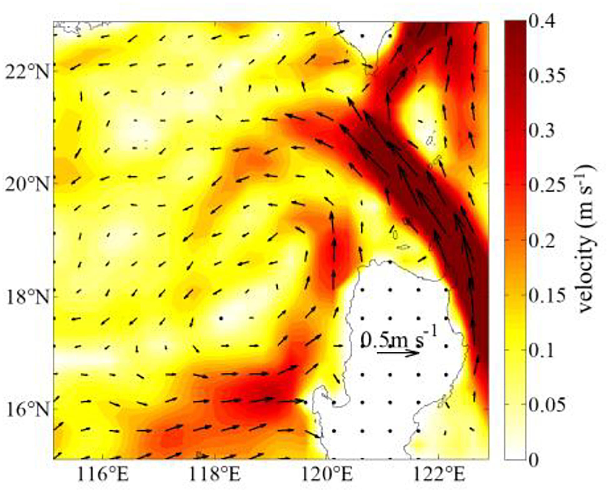
Figure 11. The geostrophic flow velocity northwest of Luzon Island. The arrow indicates the direction and size of the geostrophic flow.

The relationship among upwelling, horizontal advection by geostrophic flow, and phytoplankton bloom is supported by the vertical distribution of phosphate (Figure 6B). The center of high phosphate content is farther northward in the upper 75-m layers than that in the layers below the depth of 75 m and the location of the higher phosphate content below the depth of 75 m coincides roughly with the region of upwelling. The variation in the position of the high phosphate content at the depth of 75–100 m further suggests that the inconsistency between upwelling and phytoplankton bloom is due to horizontal advection by the geostrophic flow.

Conclusion

The present study investigated the spatial distribution and inter-annual variation of the winter phytoplankton blooms northwest of Luzon Island. The concentration of the high Chl-a patch in winter has significant partial correlations with EPV, ET, WS, SST, and SLA. However, a further analysis using the multiple stepwise correlation reveals that the wind-induced coastal upwelling (Ekman transport) and SST play more important roles in the winter Chl-a blooms than the EPV-induced upwelling (i.e., EPV), the current-induced eddy (i.e., SLA) and WS. A novel finding is that the advective effect of the geostrophic flow in the study area causes the northward deviation of the phytoplankton bloom area from the upwelling area associated with the Ekman transport and pumping. During the winter northeast monsoon, the upwelling subsurface water with abundant nutrients to the surface layer, leading to the winter phytoplankton blooms; subsequently the surface flow advects phytoplankton northward, leading to the displacement of the phytoplankton bloom center from the upwelling center induced by ET.

Data Availability Statement

Publicly available datasets were analyzed in this study. This data can be found here: Chl-a data http://hermes.acri.fr, SST products ftp://eclipse.ncdc.noaa.gov/san2/oisst/NetCDF-uncom press/, World Ocean Atlas 2018 ftp://eclipse.ncdc.noaa.gov/san2/oisst/NetCDF-uncompress/, sea surface wind http://www.remss.com/, sea surface height products http://www.aviso.altimetry.fr/duacs/, XBT profiles dataset ftp://ds1.iap.ac.cn/ftp/ds182_XBT-dataset_19662014-ChengLi Jing_0_0_netcdf/ or http://www.nodc.noaa.gov/OC5/SELECT/dbsearch/dbsearch.html.

Author Contributions

HG and HZ conceived of the presented idea. HG processed the data, performed the analysis, drafted the manuscript, and designed the figures. HZ involved in planning and supervised the funding of this work. GH helped HG and HZ to apply the stepwise method to this study. HG and HZ wrote the manuscript in consultation with GH and CD. All the authors provided critical feedback and helped shape the research, analysis and contributed to the final manuscript.

Funding

The present research is fully supported by the National Natural Science Foundation of China (No. 42076162) and the Natural Science Foundation of Guangdong Province, China (Grant No. 2020A1515010496).

Conflict of Interest

The authors declare that the research was conducted in the absence of any commercial or financial relationships that could be construed as a potential conflict of interest.

Acknowledgments

We thank GlobColor’s Working Group for providing merged Chl-a data (http://hermes.acri.fr). The National Ocean Data Center (NODC) for providing monthly SST products derived from the AVHRR (ftp://eclipse.ncdc.noaa.gov/san2/oisst/NetCDF-uncompress/), and the World Ocean Atlas 2018 climatology of nutrients and temperature data (https://www.nodc.noaa. gov/OC5/woa18/woa18data.html). The Remote Sensing Systems for providing sea surface wind (http://www.remss.com/). The AVISO project for providing sea surface height products (http://www.aviso.altimetry.fr/duacs/). And the XBT profiles dataset (ftp://ds1.iap.ac.cn/ftp/ds182_XBT-dataset_19662014-ChengLiJing_0_0_netcdf/ or http://www.nodc.noaa.gov/OC5/SELECT/dbsearch/dbsearch.html) corrected by Cheng et al. (2014) CH14 method.

Footnotes

1. ^ ftp://ds1.iap.ac.cn/ftp/ds182_XBT-dataset_19662014-ChengLiJing_0_0_netcdf/

References

Bjornsson, H., and Venegas, S. A. (1997). A Manual for EOF and SVD Analyses of Climate Data. Montréal, QC: McGill University, 52. CCGCR Report No. 97–1.

Google Scholar

Cai, S., Long, X., Wu, R., and Wang, S. (2008). Geographical and monthly variability of the first baroclinic Rossby radius of deformation in the South China Sea. J. Mar. Syst. 74, 711–720. doi: 10.1016/j.jmarsys.2007.12.008

CrossRef Full Text | Google Scholar

Chao, S. Y., Shaw, P. T., and Wu, S. Y. (1996). Deep water ventilation in the South China Sea. Deep Sea Res. Part I Oceanogr. Res. Pap. 43, 445–466. doi: 10.1016/0967-0637(96)00025-8

CrossRef Full Text | Google Scholar

Chen, C. C., Shiah, F. K., Chung, S. W., and Liu, K. K. (2006). Winter phytoplankton blooms in the shallow mixed layer of the South China Sea enhanced by upwelling. J. Mar. Syst. 59, 97–110. doi: 10.1016/j.jmarsys.2005.09.002

CrossRef Full Text | Google Scholar

Cheng, L., Zhu, J., Cowley, R., Boyer, T., and Wijffels, S. (2014). Time, probe type, and temperature variable bias corrections to historical expendable bathythermograph observations. J. Atmos. Oceanic Technol. 31, 1793–1825. doi: 10.1175/JTECH-D-13-00197.1

CrossRef Full Text | Google Scholar

Chereskin, T. K., and Price, J. F. (2001). “Ekman transport and pumping,” in Encyclopedia of Ocean Sciences, eds J. H. Steele, S. A. Thorpe, and K. K. Turekian (Amsterdam: Elsevier Science), 222–227. doi: 10.1016/B978-012374473-9.00155-7

CrossRef Full Text | Google Scholar

Eppley, R. W. (1972). Temperature and phytoplankton growth in the sea. Fish. Bull. Natl. Ocean. Atmos. Adm. 70, 1063–1085.

Google Scholar

Etourneau, J., Martinez, P., Blanz, T., and Schneider, R. (2009). Pliocene–Pleistocene variability of upwelling activity, productivity, and nutrient cycling in the Benguela region. Geology 37, 871–874. doi: 10.1130/G25733A.1

CrossRef Full Text | Google Scholar

Ganachaud, A., Vega, A., Rodier, M., Dupouy, C., Maes, C., Marchesiello, P., et al. (2010). Observed impact of upwelling events on water properties and biological activity off the southwest coast of New Caledonia. Mar. Pollut. Bull. 61, 449–464. doi: 10.1016/j.marpolbul.2010.06.042

PubMed Abstract | CrossRef Full Text | Google Scholar

García-Reyes, M., Largier, J. L., and Sydeman, W. J. (2014). Synoptic-scale upwelling indices and predictions of phyto- and zooplankton populations. Prog. Oceanogr. 120, 177–188. doi: 10.1016/j.pocean.2013.08.004

CrossRef Full Text | Google Scholar

Grimaud, G. M., Mairet, F., Sciandra, A., and Bernard, O. (2017). Modeling the temperature effect on the specific growth rate of phytoplankton: a review. Rev. Environ. Sci. Bio Technol. 16, 625–645. doi: 10.1007/s11157-017-9443-0

CrossRef Full Text | Google Scholar

Guo, L., Xiu, P., Chai, F., Xue, H., Wang, D., and Sun, J. (2017). Enhanced chlorophyll concentrations induced by Kuroshio intrusion fronts in the northern South China Sea. Geophys. Res. Lett. 44, 11,565–11,572. doi: 10.1002/2017GL075336

CrossRef Full Text | Google Scholar

G-Yull, R., and Gotham, I. J. (1981). The effect of environmental factors on phytoplankton growth: temperature and the interactions of temperature with nutrient limitation. Limnol. Oceanogr. 26, 635–648. doi: 10.4319/lo.1981.26.4.0635

CrossRef Full Text | Google Scholar

Jennrich, R. I. (1977). “Stepwise regression,” in Statistical Methods for Digital Computers, Vol. 3, eds K. Enslein, A. Ralston, and H. S. Wilf Vol (New York, NY: Wiley-Interscience), 58–75.

Google Scholar

Ledwell, J. R., Watson, A. J., and Law, C. S. (1993). Evidence for slow mixing across the pycnocline from an open-ocean tracer-release experiment. Nature 364, 701–703. doi: 10.1038/364701a0

CrossRef Full Text | Google Scholar

Liu, K. K., Chao, S. Y., Shaw, P. T., Gong, G. C., Chen, C. C., and Tang, T. Y. (2002). Monsoon-forced chlorophyll distribution and primary production in the South China Sea: observations and a numerical study. Deep Sea Res. Part I Oceanogr. Res. Pap. 49, 1387–1412. doi: 10.1016/S0967-0637(02)00035-3

CrossRef Full Text | Google Scholar

Lu, W., Yan, X. H., and Jiang, Y. (2015). Winter bloom and associated upwelling northwest of the Luzon Island: a coupled physical-biological modeling approach. J. Geophys. Res. Oceans 120, 533–546. doi: 10.1002/2014JC010218

CrossRef Full Text | Google Scholar

Maritorena, S., d’Andon, O. H. F., Manginet, A., and Siegel, D. A. (2010). Merged satellite ocean color data products using a bio-optical model: characteristics, benefits and issues. Remote Sens. Environ. 114, 1791–1804. doi: 10.1016/j.rse.2010.04.002

CrossRef Full Text | Google Scholar

Maritorena, S., and Siegel, D. A. (2005). Consistent merging of satellite ocean color data sets using a bio-optical model. Remote Sens. Environ. 94, 429–440. doi: 10.1016/j.rse.2004.08.014

CrossRef Full Text | Google Scholar

McGillicuddy, D. J. Jr., Anderson, L. A., Bates, N. R., Bibby, T., Buesseler, K. O., Carlson, C. A., et al. (2007). Eddy/Wind interactions stimulate extraordinary mid-ocean plankton blooms. Science 316, 1021–1026. doi: 10.1126/science.1136256

PubMed Abstract | CrossRef Full Text | Google Scholar

Peñaflor, E. L., Villanoy, C. L., Liu, C. T., and David, L. T. (2007). Detection of monsoonal phytoplankton blooms in Luzon Strait with MODIS data. Remote Sens. Environ. 109, 443–450. doi: 10.1016/j.rse.2007.01.019

CrossRef Full Text | Google Scholar

Phillips, O. M. (1966). “The dynamics of the upper ocean,” in Cambridge Monographs on Mechanics and Applied Mathematics, eds C. G. Batchelor, M. J. Ablowitz, S. H. Davis, E. J. Hinch, University Lecturer Damtp A Iserles J. Ockendon, et al. (Cambridge: Cambridge University Press), 261.

Google Scholar

Shang, S., Lee, Z., and Wei, G. (2011). Characterization of MODIS-derived euphotic zone depth: results for the China Sea. Remote Sens. Environ. 115, 180–186. doi: 10.1016/j.rse.2010.08.016

CrossRef Full Text | Google Scholar

Shang, S., Li, L., Li, J., Li, Y., Lin, G., and Sun, J. (2012). Phytoplankton bloom during the northeast monsoon in the Luzon Strait bordering the Kuroshio. Remote Sens. Environ. 124, 38–48. doi: 10.1016/j.rse.2012.04.022

CrossRef Full Text | Google Scholar

Shaw, P. T. (1991). The seasonal variation of the intrusion of the Philippine sea water into the South China Sea. J. Geophys. Res. 96, 821–828. doi: 10.1029/90JC02367

CrossRef Full Text | Google Scholar

Shaw, P. T., Chao, S. Y., Liu, K. K., Pai, S. C., and Liu, C. T. (1996). Winter upwelling off Luzon in the northeastern South China Sea. J. Geophys. Res. Oceans 101, 16435–16448. doi: 10.1029/96JC01064

CrossRef Full Text | Google Scholar

Siegel, H., Ohde, T., Gerth, M., Lavik, G., and Leipe, T. (2007). Identification of coccolithophore blooms in the SE Atlantic Ocean off Namibia by satellites and in-situ methods. Continental Shelf Res. 27, 258–274. doi: 10.1016/j.csr.2006.10.003

CrossRef Full Text | Google Scholar

Tang, D. L., Kawamura, H., Dien, T. V., and Lee, M. A. (2004). Offshore phytoplankton biomass increase and its oceanographic causes in the South China Sea. Mar. Ecol. Prog. 268, 31–41. doi: 10.3354/meps268031

CrossRef Full Text | Google Scholar

Tang, D. L., Kester, D. R., Ni, I. H., Kawamura, H., and Hong, H. (2002). Upwelling in the Taiwan Strait during the summer monsoon detected by satellite and shipboard measurements. Remote Sens. Environ. 83, 457–471. doi: 10.1016/S0034-4257(02)00062-7

CrossRef Full Text | Google Scholar

Tang, D. L., Ni, I. H., Kester, D. R., and Muller-Karger, F. E. (1999). Remote sensing observations of winter phytoplankton blooms southwest of the luzon strait in the South China Sea. Mar. Ecol. Prog. 191, 43–51. doi: 10.3354/meps191043

CrossRef Full Text | Google Scholar

Tremblay, J. É, Bélanger, S., Barber, D. G., Asplin, M., Martin, J., Darnis, G., et al. (2011). Climate forcing multiplies biological productivity in the coastal Arctic Ocean. Geophys. Res. Lett. 38, 113–120. doi: 10.1029/2011GL048825

CrossRef Full Text | Google Scholar

Wang, J. J., Tang, D. L., and Sui, Y. (2010). Winter phytoplankton bloom induced by subsurface upwelling and mixed layer entrainment southwest of Luzon Strait. J. Mar. Syst. 83, 141–149. doi: 10.1016/j.jmarsys.2010.05.006

CrossRef Full Text | Google Scholar

Wu, J., Chung, S. W., Wen, L.-S., Liu, K. K., Chen, Y. L. L., Chen, H. Y., et al. (2003). Dissolved inorganic phosphorus, dissolved iron, and Trichodesmium in the oligotrophic South China Sea. Glob. Biogeochem. Cycles 17:1008. doi: 10.1029/2002GB001924

CrossRef Full Text | Google Scholar

Xu, Y., Chant, R., Gong, D., Castelao, R., Glenn, S., and Schofield, O. (2011). Seasonal variability of chlorophyll a in the Mid-Atlantic Bight. Cont. Shelf Res. 31, 1640–1650. doi: 10.1016/j.csr.2011.05.019

CrossRef Full Text | Google Scholar

Zhao, H., Sui, D., Xie, Q., Han, G., Wang, D., Chen, N., et al. (2012). Distribution and interannual variation of winter phytoplankton blooms northwest of Luzon Islands from satellite observations. Aquat. Ecosyst. Health Manag. 15, 53–61. doi: 10.1080/14634988.2012.648875

CrossRef Full Text | Google Scholar

Zhao, H., and Tang, D. L. (2007). Effect of 1998 El Niño on the distribution of phytoplankton in the South China Sea. J. Geophys. Res. 112, 117–128. doi: 10.1029/2006JC003536

CrossRef Full Text | Google Scholar

Zhao, H., and Wang, Y. (2018). Phytoplankton increases induced by tropical cyclones in the South China Sea during 1998–2015. J. Geophys. Res. 123, 2903–2920. doi: 10.1002/2017JC013549

CrossRef Full Text | Google Scholar

Zhou, C., Zhao, W., Tian, J., Yang, Q., and Qu, T. (2014). Variability of the deep-water overflow in the luzon strait^∗. J. Phys. Oceanogr. 44, 2972–2986. doi: 10.1175/JPO-D-14-0113.1

CrossRef Full Text | Google Scholar