Energetics of Eddy-Mean Flow Interactions in the Amery Ice Shelf Cavity

Introduction

The Amery Ice Shelf (AIS) is the third largest Antarctic ice shelf located in East Antarctica, with an area of about 62,000 km² (Herraiz-Borreguero et al., 2016a). The AIS is mainly fed by the Lambert-Mellor-Fisher tributary glacial systems (Wen et al., 2007; Yu et al., 2010), and it contains some of the deepest Antarctic floating ice (more than 2,500 m below sea level; Fricker et al., 2000). Antarctic ice shelves are key for global sea level rise and Southern Ocean circulation, by exchanging mass, heat, and salt with the Southern Ocean (Heil et al., 1996; Williams et al., 2002; Shepherd et al., 2010; Joughin and Alley, 2011; Pritchard et al., 2012). In addition, the ocean circulation under the AIS also has great impacts on marine bio-geochemical and ecological processes (Williams et al., 2010; Post et al., 2014; Herraiz-Borreguero et al., 2016b).

To better understand the important impacts of ocean-ice shelf interaction on the Antarctic climate system and ecosystem, a deeper understanding of ocean dynamics in the sub-ice-shelf cavity is essential. For this purpose, we conducted a thorough examination of the eddy-mean flow interaction by analyzing the Lorenz energy cycle (LEC). LEC is a useful method to analyze the oceanic and atmospheric energy cycle and corresponding dynamic processes (Lorenz, 1955; Oort and Peixoto, 1983; Oort et al., 1994; Wunsch and Ferrari, 2004). For example, using a number of ocean observations, Oort et al. (1994) analyzed the energetics of the global ocean including energy generation, conversion and dissipation terms, and Wunsch and Ferrari (2004) depicted major energy reservoirs and energy dissipation mechanisms. Based on fully compressible Navier-Stokes equations, Tailleux (2009) developed the framework of available potential energy (APE), despite the challenging nature of the accurate definition of APE (Huang, 2005); and the importance of buoyancy power input has been highlighted (Tailleux, 2010). In the sub-ice-shelf cavity, for example, the buoyancy power input supplies almost all the energy to drive the circulation as wind stress cannot be exerted on sea water (Foldvik and Kvinge, 1974; Lewis, 1985; Schodlok et al., 2016).

Benefitting from high-resolution numerical models, detailed investigations of the global ocean energy cycle have been advanced (Cox, 1985; Liang and Robinson, 2005, 2007; Maltrud et al., 2010; Lucarini and Ragone, 2011; Olbers et al., 2012; von Storch et al., 2012; Chen et al., 2014; Kang and Curchitser, 2015; Zemskova et al., 2015; Yang and Liang, 2016; Wu et al., 2017a, 2021). For example, Wu et al. (2017a) analyzed the response of the LEC for the Southern Ocean to intensified westerlies. They found that all energy conversions are enhanced under stronger wind forcing, and the conversion rates in the Southern Ocean are strongly influenced by large topography where energy is converted from eddy kinetic energy (EKE) to mean kinetic energy (MKE). In addition, a number of studies (Eden and Boning, 2002; Xie et al., 2007; Shore et al., 2008; Zhai et al., 2010; Yang et al., 2013; Kang and Curchitser, 2015, 2016; Zhan et al., 2016) have also investigated the energetics of a regional ocean using a similar method as that used in von Storch et al. (2012) and Wu et al. (2017a). These investigations found that the eddies are generated by two pathways: the barotropic pathway (where MKE transfers energy directly to EKE) and the baroclinic pathway (where eddies gain energy from available potential energy), with the baroclinic pathway being dominant (Kang and Curchitser, 2015; Wu et al., 2017a, 2021). Recently, model results and observations have demonstrated that eddy processes play an important role in transporting warm Circumpolar Deep Water (CDW) onto the continental shelf where it can enter the ice shelf cavity (Moffat et al., 2009; Martinson and McKee, 2012; Stewart and Thompson, 2015; Couto et al., 2017). St-Laurent et al. (2013) also found that eddies are necessary to represent the interaction between a Rossby wave along the shelf break and a bathymetric trough, leading to trough-induced intrusions of CDW. The importance of eddy-mediated heat transfer onto the continental shelf has also been found in the East Antarctic, Amundsen Sea, western Antarctic Peninsula, and Prydz Bay by realistic ocean models (Hattermann et al., 2014; Nakayama et al., 2014; St-Laurent et al., 2015; Graham et al., 2016; Liu et al., 2017). In addition, a comprehensive modeling study of on-shelf heat transport around Antarctica found that eddies drive the net shoreward heat transport onto the continental shelves (Stewart et al., 2018). However, a detailed investigation on the eddy-mean flow interaction in an Antarctic sub-ice-shelf cavity has not been conducted so far. One principal difficulty arises from the limited spatial and temporal coverage of oceanographic observational data underneath Antarctic ice shelves. Another difficulty is that the typical value of Rossby deformation radius is about 5 km on the Antarctic continental shelves (Hallberg, 2013; Nurser and Bacon, 2014; Mack et al., 2019) and hence most models with coarse spatial resolutions cannot fully resolve eddies on the Antarctic continental shelves and in sub-ice-shelf cavities (Wu et al., 2017a; Mack et al., 2019). Closer to the ice shelf front, the brine rejection induced by sea ice formation, especially in polynya regions, is key to the water mass transformation by increasing salinity and mediating surface freezing point (Naughten et al., 2019). Thus, the detailed investigation of eddy-mean flow interaction in a sub-ice-shelf cavity requires a high-resolution coupled ocean-sea ice-ice shelf model.

There are also a number of differences between the energy cycles in a sub-ice-shelf cavity and the open ocean. In the open ocean, the ocean general circulation is driven by external forcing such as the winds, tides, the exchanges of heat and freshwater with the atmosphere; particularly, the wind supplies most energy to the ocean circulation (Wunsch, 1998; Huang et al., 2006; von Storch et al., 2007; Hughes and Wilson, 2008; Scott and Xu, 2009; Wu et al., 2016, 2017b), and most of that is deposited into the Southern Ocean (Roquet et al., 2011; Zhai et al., 2012; Wu et al., 2017a, 2020). However, as mentioned above, wind power input cannot be exerted on sea water beneath an ice shelf. Instead, the ice pump mechanism mainly drives the circulation in the vast majority of big sub-ice-shelf cavities (Foldvik and Kvinge, 1974; Lewis, 1985; Schodlok et al., 2016). The ice pump mechanism involves freshwater generation by ice shelf melting resulting in an increase of buoyancy and then generating kinetic energy. The increase in the freezing with the ascending water can lead to direct marine ice accretion with subsequent brine rejection which might in turn modify the in situ ocean condition. Hence, a quantitative analysis of the ice pump mechanism through investigating the eddy-mean flow interaction is useful for understanding the unique dynamics in a sub-ice-shelf cavity.

In Prydz Bay, the main ocean circulation is characterized by a large cyclonic gyre, centered in the Amery Depression (Smith et al., 1984; Nunes Vaz and Lennon, 1996). Previous numerical studies have simulated the ocean circulation in Prydz Bay and beneath the AIS (Williams et al., 2001; Galton-Fenzi et al., 2012; Liu et al., 2017). The cyclonic Prydz Bay gyre is reproduced in the previous numerical simulations; these simulations further suggest the existence of cyclonic circulation beneath the ice shelf, i.e., inflow of dense shelf waters in the eastern flank of the cavity and outflow of cold and low salinity Ice Shelf Water (ISW) in the western flank (Figure 1). The inflow of modified CDW along the eastern flank of the AIS can induce a basal melting rate of up to 2 m yr^–1 at the northeastern corner of the AIS (Herraiz-Borreguero et al., 2015).

FIGURE 1

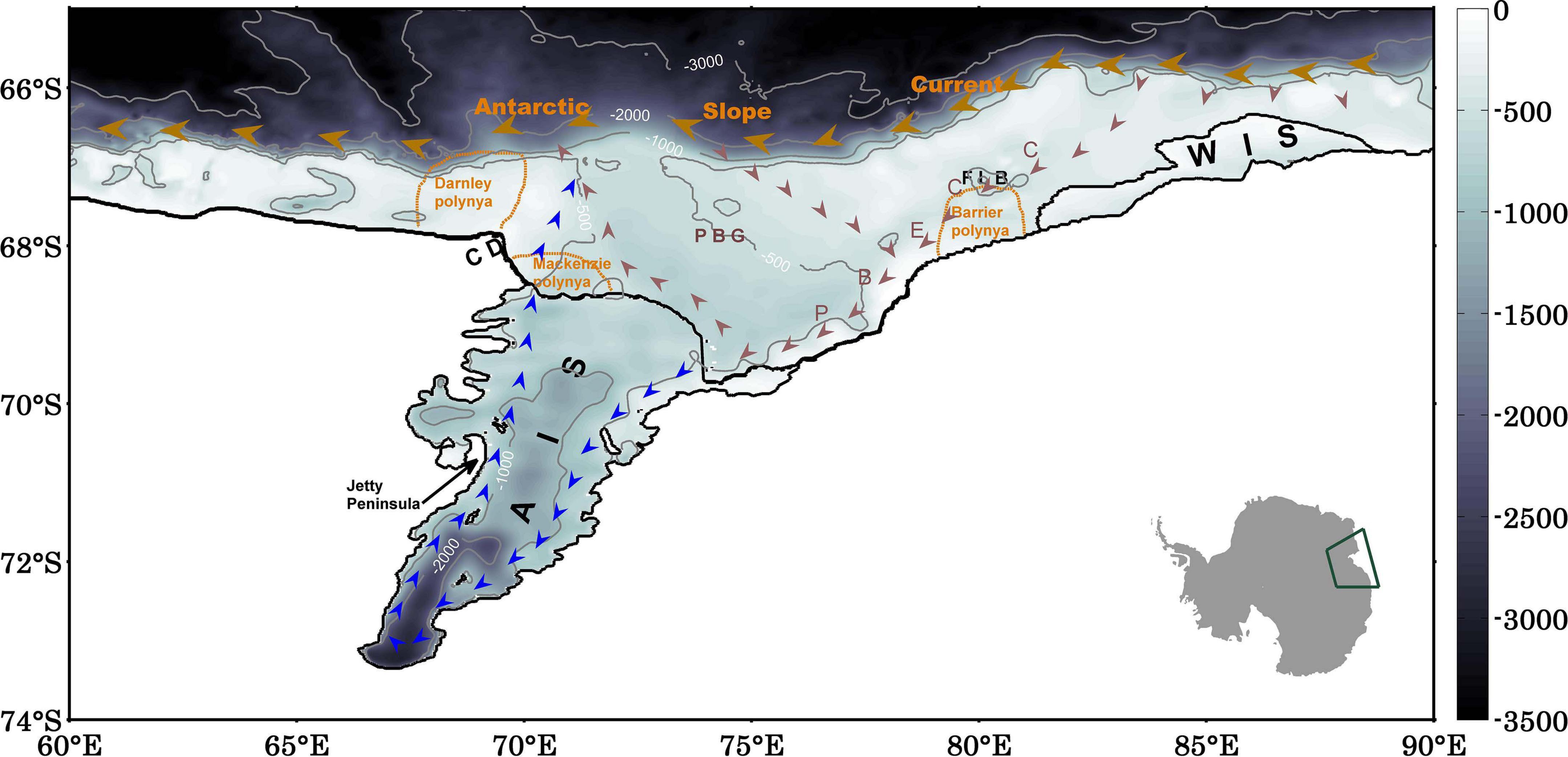
Figure 1. A schematic diagram of the general ocean circulation in Prydz Bay and underneath the Amery Ice Shelf. The orange dashed lines show the locations of Darnley, Barrier and Mackenzie polynyas. The color scale shows the water column thickness in unit of m. The contours show the bathymetry. Inset: the location of Prydz Bay and the Amery Ice shelf in East Antarctica.

In this paper, we used the outputs of a recently developed eddy-resolving ocean-sea ice-ice shelf model (Liu et al., 2017) to conduct a quantitative study on the LEC in the sub-ice-shelf cavity of the AIS. The remainder of this paper is structured as follows. Sections “Materials and Methods” and “Results” provide brief descriptions of the theoretical framework and the numerical model used in this study. The detailed analysis of the eddy-mean flow energetics under the AIS is presented in section “Results”. This paper is summarized with a conclusion and discussion in section “Concluding Remarks and Discussion”.

Materials and Methods

Diagnostic Framework

Following von Storch et al. (2012) and Wu et al. (2017a), the four energy reservoirs, namely, MKE (_km), EKE (_ke), mean available potential energy (MAPE,_Pm), eddy available potential energy (EAPE, _Pe), are defined as follows:

$MKE(k_m)=\frac{1}{2}{\mathrm{\rho }}_0({\overline{u}}^2+{\overline{v}}^2),(1)$

$\text{EKE}(k_e)=\frac{1}{2}{\mathrm{\rho }}_0(\overline{u^{\prime 2}+v^{\prime 2}}),(2)$

$\text{MAPE}(P_m)=-\frac{g}{2n_0}\overline{{\mathrm{\rho }}^{*2}},\text{and}(3)$

$\text{EAPE}(P_e)=-\frac{g}{2n_0}\overline{{\mathrm{\rho }}^{\prime 2}},(4)$

where _ρ0 is a constant reference density (1,038 kg m^–3), _u is the zonal velocity, and _v is the meridional velocity, with the over bar denoting monthly means over the 5-year period and the prime denoting the deviation from these time means, as the general life period of the eddy activities in the AIS cavity is less than 1 week. It will be shown later that the annual cycle makes large contributions to the eddy reservoirs and the associated energy conversion terms in the AIS cavity especially near the ice front region (Dinniman et al., 2015), if the annual cycle is included in the eddy terms. n₀ is the vertical gradient of the time (monthly) and area mean (over the whole AIS cavity) of local potential density ρ, which can be split into two parts, as following$\mathrm{\rho }(x,y,z,t)={\mathrm{\rho }}^{*}(x,y,z,t)+<\overline{\mathrm{\rho }(x,y,z,t)}>$; and, < ⁣⋅⁣ > represents the total area mean at a given depth. $<\overline{\mathrm{\rho }(x,y,z,t)}>$ is the reference density defined by the whole area average of the monthly density over the AIS cavity. The value of n₀is different for each month. It is noted that this definition of APE is just an approximation, particularly in the regions with weak stratification and big topography (Stewart et al., 2014; Zemskova et al., 2015). The MAPE field is found to be sensitive to the choice of density reference stratification (ρ_r). Both its spatial distribution and integrated value change largely when evaluated with alternative ρ_r profiles, especially for the one over the region near the ice shelf front (not shown). However, the density reference stratification has a negligible influence on EAPE and the associated conversion rates (_MAPE→EAPE and _MAPE→MKE; not shown).

Briefly, the dissipation terms of KE induced by the drag stress at ice shelf base and bottom topography, and the generation terms of APE are given by

$\text{D}(k_m)=\overline{{\mathrm{\tau }}_{IS}}\overline{{\mathbf{\text{u}}}_{IS}}+\overline{{\mathrm{\tau }}_{\text{B}}}\overline{{\mathbf{\text{u}}}_{\text{B}}},(5)$

$D(k_e)=\overline{{\mathrm{\tau }}_{IS}^{\prime }{\mathbf{\text{u}}}_{IS}^{\prime }}+\overline{{\mathrm{\tau }}_{\text{B}}^{\prime }{\mathbf{\text{u}}}_{\text{B}}^{\prime }},(6)$

$G(P_m)=-\frac{\overline{{\mathrm{\rho }}^{*}}}{n_0}{\overline{B}}_0,(7)$

and

$G(P_e)=-\overline{\frac{{\mathrm{\rho }}^{\prime }}{n_0}{B}^{\prime }},(8)$

where _τIS and _τB denote the horizontal ice shelf-ocean drag stress and bottom drag stress, _uIS and _uB are the ice shelf-ocean interface horizontal velocity and the bottom horizontal velocity, $B_0=\frac{g}{{\mathrm{\rho }}_0}(\frac{\mathrm{\alpha }{Q}^{*}}{C_w}+{\mathrm{\rho }}_0\mathrm{\beta }S{E}^{*})$, $\mathrm{\alpha }={(\frac{\partial \mathrm{\rho }}{\partial \mathrm{\theta }})}_{S,z}$, $\mathrm{\beta }={(\frac{\partial \mathrm{\rho }}{\partial S})}_{\mathrm{\theta },z}$, θ and S denote the potential temperature and salinity, _Cw is the heat capacity of seawater, _Q^* and _E^* are the net ice shelf-ocean heat and freshwater fluxes. Note that wind stress does not supply wind power to the sea water beneath the AIS; conversely, the ice shelf-ocean and the bottom drag stresses (Eqs. 5, 6), which are estimated using the quadratic bulk formula (Hibler and Bryan, 1987; McPhee, 2008), extract KE from the ocean. And, the quadratic drag coefficients at the ice shelf and sea bed are set as 2 × 10^–3. Note that the dissipation terms of KE are just approximations, as it can also be dissipated through interior vertical viscosity and biharmonic viscosity in this model (Wu et al., 2017a).

In addition, the conversion terms are the following:

$C(k_m,k_e)=-{\mathrm{\rho }}_0(\overline{u^{\prime }{u}^{\prime }}\cdot \nabla \overline{u}+\overline{v^{\prime }{u}^{\prime }}\cdot \nabla \overline{v}),(9)$

$C(P_e,P_m)=-\frac{g}{n_0}\overline{{\mathrm{\rho }}^{\prime }{u}^{\prime }}\cdot \nabla \overline{{\mathrm{\rho }}^{*}},(10)$

$C(P_m,k_m)=-g\overline{{\mathrm{\rho }}^{*}}\overline{w},(11)$

and

$C(P_e,k_e)=-g\overline{{\mathrm{\rho }}^{\prime }{w}^{\prime }},(12)$

where _w is the vertical velocity, _u and _uh denote the three-dimensional and horizontal velocity vectors. The positive value of C (A, B) means the energy is converted from A to B. Conversely, a negative value of C (A, B) means the energy is converted from B to A. The lateral transport terms of MKE (_B(km)), EKE (_B(ke)), MAPE (_{B (Pm)}), and EAPE (_{B (Pe)}) are given by

$B(k_m)={\int }_{{\mathrm{\Omega }}_N}(\overline{v}{k}_m+\overline{v}\overline{p})\mathit{d}S,(13)$

$B(k_e)={\int }_{{\mathrm{\Omega }}_N}(\overline{(v\frac{1}{2}{\mathrm{\rho }}_0(u^{\prime 2}+v^{\prime 2}))}+\overline{v^{\prime }{p}^{\prime }})\mathit{d}S,(14)$

$B(P_m)={\int }_{{\mathrm{\Omega }}_N}\overline{v}{P}_m\mathit{d}S,(15)$

and

$B(P_e)={\int }_{{\mathrm{\Omega }}_N}\overline{v{P}_e}\mathit{d}S,(16)$

where_pis the pressure, _ΩN denotes the northern boundary at the AIS calving front. We refer readers to Wu et al. (2017a) for the detailed derivation of the energy budget equations used here.

Model

A high-resolution coupled regional ocean-sea ice-ice shelf model (Liu et al., 2017) is used to investigate the energetics under the AIS based on the equations given in section “Materials and Methods.” The simulation is performed using the Massachusetts Institute of Technology General Circulation Model (MITgcm; Marshall et al., 1997a,b; Losch, 2008), which solves the primitive equations with the Boussinesq approximation and hydrostatic assumption. The model domain extends from 74 to 65 S and from 60 to 90 E with a spherical grid projection, including Prydz Bay and the AIS cavity (Figure 1). The mean zonal and meridional grid spacings of the model are 0.045° and 0.014°, respectively. Hence, the zonal grid spacing is between 1.4 and 2.2 km at the southern and northern boundaries, respectively, and the meridional grid spacing is 1.5 km. In addition, there are 70 unevenly spaced vertical levels whose thickness increases from 10 m near the surface to 250 m near the ocean bottom. This high-resolution horizontal grid spacing is necessary for resolving meso-scale eddies, as the Rossby radius of deformation here is only a few kilometers (Mack et al., 2019). Note that it can become less than 1 km, especially in destratified water column as commonly observed under cold ice shelves in polar winter condition (Nurser and Bacon, 2014; Mack et al., 2019). With our model resolution a majority of mesoscale eddies can be captured in the AIS cavity; It cannot capture all eddies with scales down to 1 km which could decrease shelf transport of modified CDW (St-Laurent et al., 2013; Stewart and Thompson, 2015; Mack et al., 2019). The ice draft and bathymetry used here are obtained from a global 1-min Refined Topography data set (RTopo-1) (Timmermann et al., 2010), which has the deepest part of the AIS being about 2,500 m and the water column thickness greater than 1,500 m (Figure 1). The model allows the ice shelf to move up and down in hydrodynamic balance with the ocean.

The horizontal sub-grid-scale viscosity and diffusion is set as strain rate-dependent diffusivity (Smagorinsky, 1963). The background mixing of potential temperature and salinity is realized by a vertical diffusivity of 5 × 10^–7 m² s^–1, supplemented by the K-Profile Parameterization (Large et al., 1994). Bottom stress is parameterized using the quadratic drag law; and the quadratic drag coefficients at the ice shelf and sea bed are set as 2 × 10^–3 (Griffies and Hallberg, 2000). The dissipation rate of kinetic energy will change with different quadratic drag coefficients. The oceanic equation of state is the same as that used in Jackett and McDougall (1995). The parameterization used to model the ice-ocean thermodynamic exchanges are obtained from solving a system of three equations that is derived from the heat and freshwater balance at the ice ocean interface (Hellmer and Olbers, 1989; Holland and Jenkins, 1999; Jenkins et al., 2001; Losch, 2008; Naughten et al., 2019). The transfer coefficients for temperature and salinity at the ice shelf-ocean interface are functions of the friction velocity (Holland and Jenkins, 1999; Dansereau et al., 2014). This model does not explicitly include tides. This flaw may lead to a weaker eddy activity and lower freezing/melting rates (Liu et al., 2017; Mueller et al., 2018). The vertical diffusivity and viscosity coefficients of 10^–5 m² s^–1 and 10^–4 m² s^–1 are applied, respectively. It can partially mimic the tide mixing, as used in Naughten et al. (2019). Details of the model configuration and the model assessments can be found in Liu et al. (2017).

Experiments

The model was spun up for 20 years using the monthly climatology (averaged over 1979–2012) of the atmospheric data from the Japanese Reanalysis (JRA-55) dataset at a spatial resolution of 1.125°× 1.125° (Kobayashi et al., 2015). After the 20-yr spin-up phase, the kinetic energy in the sub-ice-shelf cavity reaches a steady state (Liu et al., 2017). Afterward, the simulation (CONTROL) is integrated for another 5 years (1979–1983) driven by the 6-hourly atmospheric forcing and the 1-day mean outputs for these 5 years were analyzed in this study. The JRA-55 used here includes net long wave radiation, net shortwave radiation, humidity, 2 m air temperature, precipitation, and 10 m winds. The monthly eastern, western and northern boundary conditions are specified by the outputs from the Estimating the Circulation and Climate of the Ocean phase II: high resolution global-ocean and sea-ice data synthesis (ECCO2) (Menemenlis et al., 2008). Benefiting from hydrographic and satellite observations, the model performance has been assessed in Liu et al. (2017).

To further diagnose the influence of the ice pump mechanism on the LEC beneath the AIS, another experiment (Exp-shutdown) has been conducted. The only difference from the CONTROL experiment is that the thermodynamic influence of the AIS on the ocean is excluded in Exp-shutdown, i.e., the heat and freshwater fluxes at the ice shelf-ocean interface are set to zero. Unless otherwise stated, model outputs from CONTROL over the last 5 years are used for this study. And, the annual means of energy reservoirs and conversion rates are analyzed.

Results

Energy Reservoirs

Figure 2 shows the annual mean distributions of the vertically integrated MKE (Figure 2A), EKE (Figure 2B), MAPE (Figure 2C) and EAPE (Figure 2D). Two subdomains representing the inner (AIS1) and outer (AIS2) parts of the sub-ice-shelf cavity are outlined and labeled in Figure 2B. All four energy components exhibit distinctive spatial patterns. The distribution of MKE is dominated by two narrow strips of large MKE along the eastern and western flanks of the AIS cavity, with the MKE on the eastern side being weaker than that on the western side in the AIS2 region (Figure 2A). As the kinetic energy mainly concentrates in the ocean circulation, the distribution of MKE reflects the main cyclonic circulations beneath the ice shelf, i.e., inflow of shelf water in the east and outflow of ISW in the west (Williams et al., 2001, 2002; Hemer et al., 2006; Galton-Fenzi et al., 2012). The relatively large MKE in the eastern flank in the outer part (AIS2) reflects the simulated intrusion of the outside water until 70 S, while the re-emerging of large MKE in the inner part (AIS1) is apparently driven by the ice pump mechanism (Figure 2A).

FIGURE 2

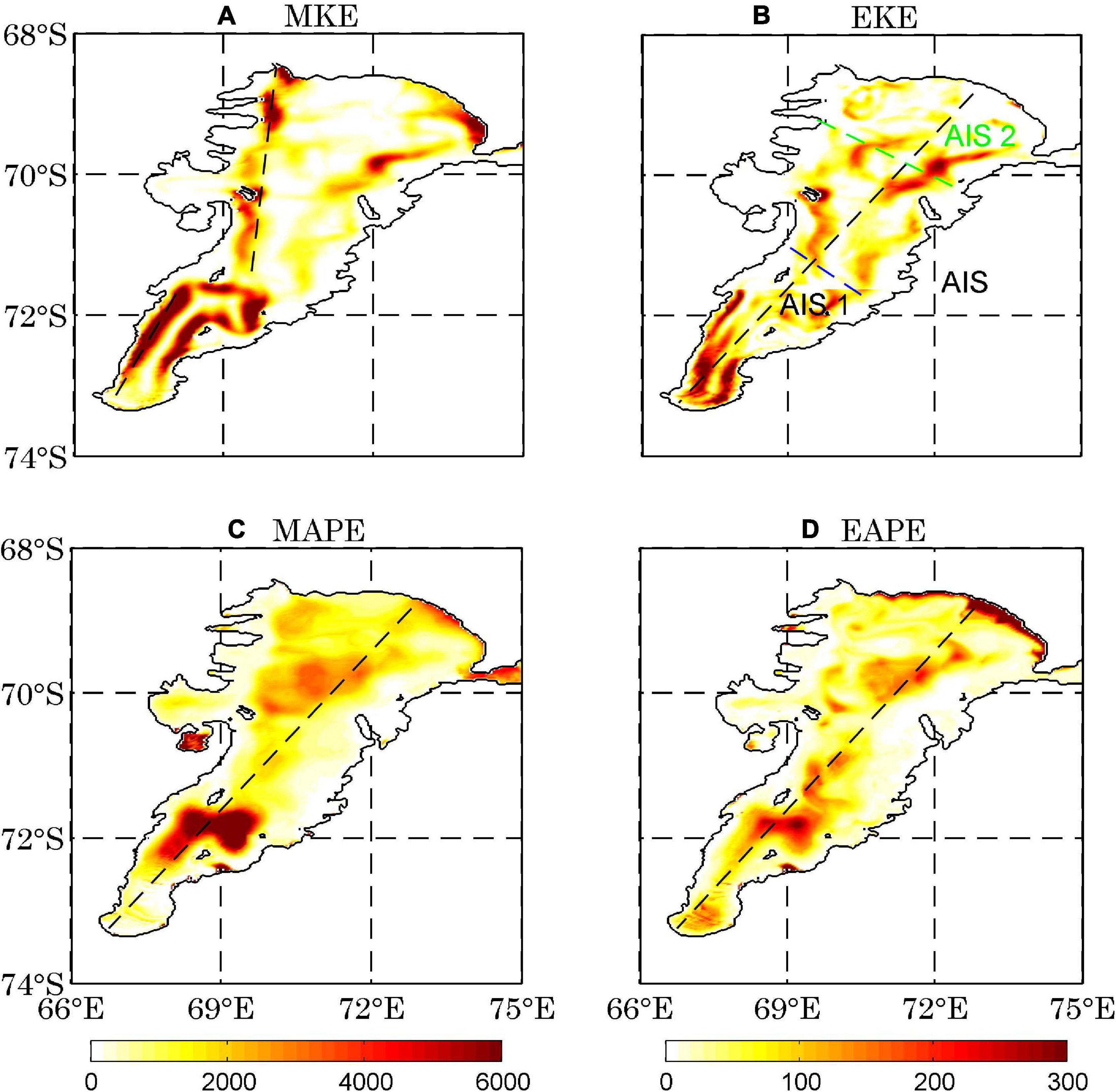
Figure 2. The annual mean distributions of the vertically integrated energy components (J m^–2). The black dashed lines in (A–D) mark the locations of the vertical cross sections in Figure 5. The inner and outer subdomains are outlined by the blue and green lines and marked by AIS1 and AIS2, respectively, in Figure 2B.

The EKE shows a different pattern from MKE, characterized by large and well spread EKE in the interior areas, especially in regions AIS1 (Figure 2B). Large EKE on the eastern side of AIS2 is induced by the flow of EKE from the outside. Large EKE also exists in region AIS1, especially near the grounding line where the maximal melt rate is about 30 m yr^–1 (Wen et al., 2007; Galton-Fenzi et al., 2012). The remarkable release of freshwater near the grounding line makes the seawater buoyant; hence, APE is available to generate vigorous eddy activity there. When the seawater ascends along the upward-sloping base of the ice shelf, refreezing of this water diminishes buoyancy through brine rejection. Notably, the large EKE is also concentrated in the depression region near 72 S (Figure 1) where MKE (Figure 2A), MAPE (Figure 2C), and EAPE (Figure 2D) are also large, implying strong barotropic and baroclinic instability there. In addition, the relative vorticity shows that abundant eddies exist in the AIS cavity, especially in the regions near the boundaries and the ice front (not shown). There are substantial high-frequency variabilities in time series of temperature, salinity and velocities at the top two model levels in the AIS cavity (not shown). Power spectra analysis of these high-frequency fluctuations show that the most visible period is from 2 to 6 days (not shown).

Figures 2C,D show the distributions of vertically integrated MAPE and EAPE, respectively. Broadly, the pattern of EAPE is similar to that of MAPE. The MAPE and EAPE distributions feature larger values in region AIS2 and the region around 72 S than in region AIS1. The ocean gains large MAPE in the eastern AIS calving front caused by basal melt of up to 2 m yr^–1 (melting causes an increase in MAPE in the form of buoyancy release; Herraiz-Borreguero et al., 2015); Another region of high MAPE is near the grounding line which is induced by basal melting as large as 30 m yr^–1, consistent with previous modeling studies (Galton-Fenzi et al., 2012). Also, the pattern of EAPE is basically similar to that of EKE, especially in region AIS1. The resemblance of the horizontal structure between EAPE and EKE was also found in the global ocean and the Southern Ocean (Roullet et al., 2014; Wu et al., 2017a). It will be shown later that the similar spatial distributions of these three reservoirs (MAPE, EAPE, and EKE) imply that the energy under the ice shelf mainly transfers through the baroclinic pathway, especially near 72 S.

The eddy term is redefined to examine the effect of annual cycle on the reservoirs and the associated energy conversion terms. The “mean” denotes time mean over the 5-yr model outputs and the “eddy” denotes the deviation from this annual mean. Variables included the annual cycle are defined as “variable_{_annual}.” When the seasonal cycle is included, the patterns of eddy reservoirs change slightly except the AIS2 region (Figure 3). Also, the life period of the eddies in the AIS cavity is less than 1 week (not shown). Hence, the monthly mean is chosen to decompose the “mean” and the “eddy” in this study. In addition, the volume integrated values of EKE and EKE_{_annual} are 5.5 TJ to 15.7 TJ, respectively; the volume integrated EAPE and EAPE_{_annual} increase from 10.1 to 34.9 TJ when the annual cycle is included. Additionally, the new defined eddy term shows that the annual cycle accounts for roughly 60% of variability in the G(EAPE_{_annual}), D(EKE_{_annual}) and the associated conversion terms (_{MAPE__ annual →EAPE__ annual →EKE__ annual} and _{MKE__ annual→EKE__ annual}), especially in the AIS front region (not shown). These results further indicate suppressed eddy activities in a sub-ice-shelf cavity as both the stresses at the ice shelf base and bottom topography dissipate the kinetic energy.

FIGURE 3

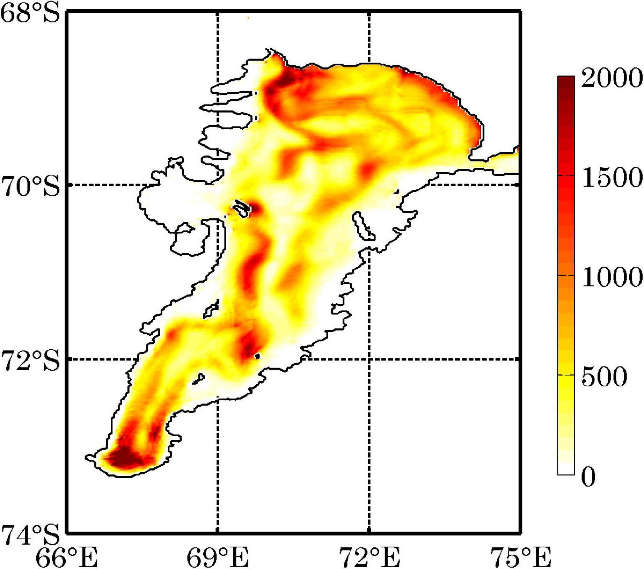
Figure 3. The annual mean distributions of the vertically integrated EKE_{_annual} (J m^–2). Note that the time-mean used here is the 5-year mean which is different from monthly mean used in Figure 2B.

The sections across the areas with large reservoirs are chosen to illustrate the vertical distributions of the four energy components; both the MKE and EKE extend throughout the whole water column (Figures 4A,B). Larger MKE concentrates in the inner part of the ocean cavity from the ice shelf draft to bedrock (Figure 4A); large EKE can also be identified throughout the whole water column near the grounding line (Figure 4B). In contrast, large MAPE and EAPE concentrate near the base of the AIS. It is interesting to note that the relatively large MAPE and EAPE in the region from 69 to 70 S (Figures 4C,D) result from strong transports of MAPE and EAPE from near the grounding line where large buoyancy power input exists (see below). The corresponding EKE increase shifts to the eastern side of this selected cross section (Figure 2). The basal melting only occurs at the interface between the ice shelf base and ocean water. Hence, APE is confined mostly to the upper water column (Figures 4C,D). When the APE is transferred to the kinetic energy, the vertical structure of the mean circulation and eddy activity extends through the column (Figures 4A,B). The down sloping feature at 71.5 E in the EAPE is most likely induced by large eddy activity present in this location (Figure 4D).

FIGURE 4

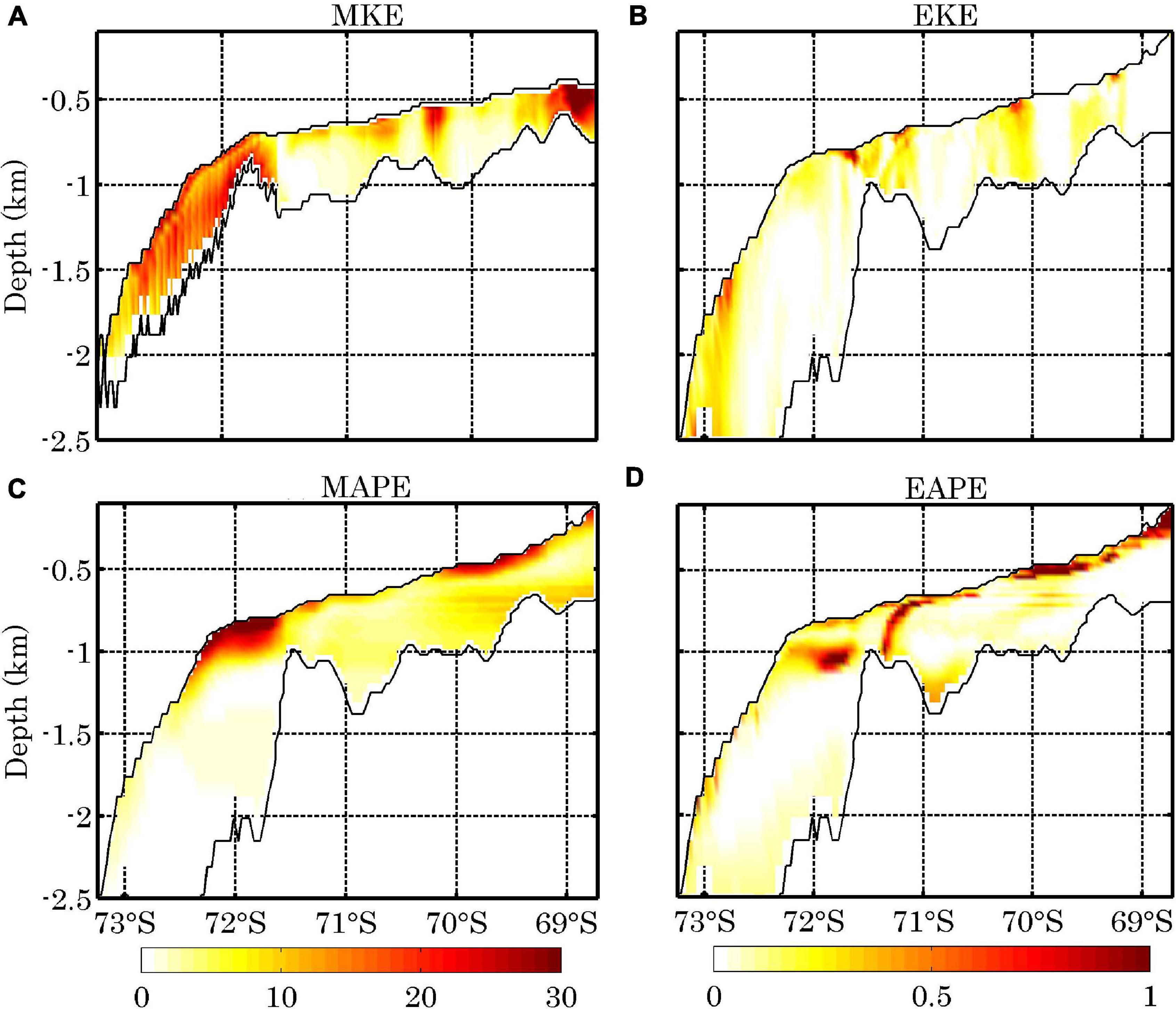
Figure 4. The annual mean vertical distributions of MKE (A, J m^–3), EKE (B, J m^–3), MAPE (C, J m^–3), and EAPE (D, J m^–3) along the sections indicated in Figure 2. Note that the location of the vertical cross section of MKE is different from those of MAPE, EAPE, and EKE.

The magnitudes of averaged MKE over the whole AIS domain generally decrease toward the deeper ocean (Figure 5A), except in the upper 200 m. The profile of EKE is visibly different from that of MKE in such a way that the EKE decreases dramatically in the upper 600 m, and then changes slightly below 1,000 m. Another feature is that the area average MKE is larger than EKE in almost all the model layers except the upper layers. This is contrast to earlier findings that EKE is much more dominant than MKE in most areas of the Southern Ocean (Wu et al., 2017a) and the global ocean (von Storch et al., 2012), reflecting again that eddies are greatly suppressed by both the stresses at ice shelf base and bottom topography. The larger MKE reservoir than EKE reflects that the current under the AIS, driven by the ice pump mechanism, is steadier than that in the open ocean. It is noted that EKE is larger than MKE in the upper tens of meters which is presumably influenced by the combined effects of CDW, dense shelf water (DSW), ISW, the formation of marine ice, and the vertical shear. The area average MAPE and EAPE (Figure 5A) over the AIS cavity are different from each other: above 150 m, MAPE increases with depth and decreases dramatically below, whereas EAPE decreases with depth dramatically above 200 m and shows a moderate decrease below; in addition, MAPE is much larger than EAPE. The vertical profile of EAPE is roughly similar to that of EKE, implying that the energy exchange between these reservoirs is dominated by the baroclinic pathway (i.e., _{MAPE→EAPE→ EKE}).

FIGURE 5

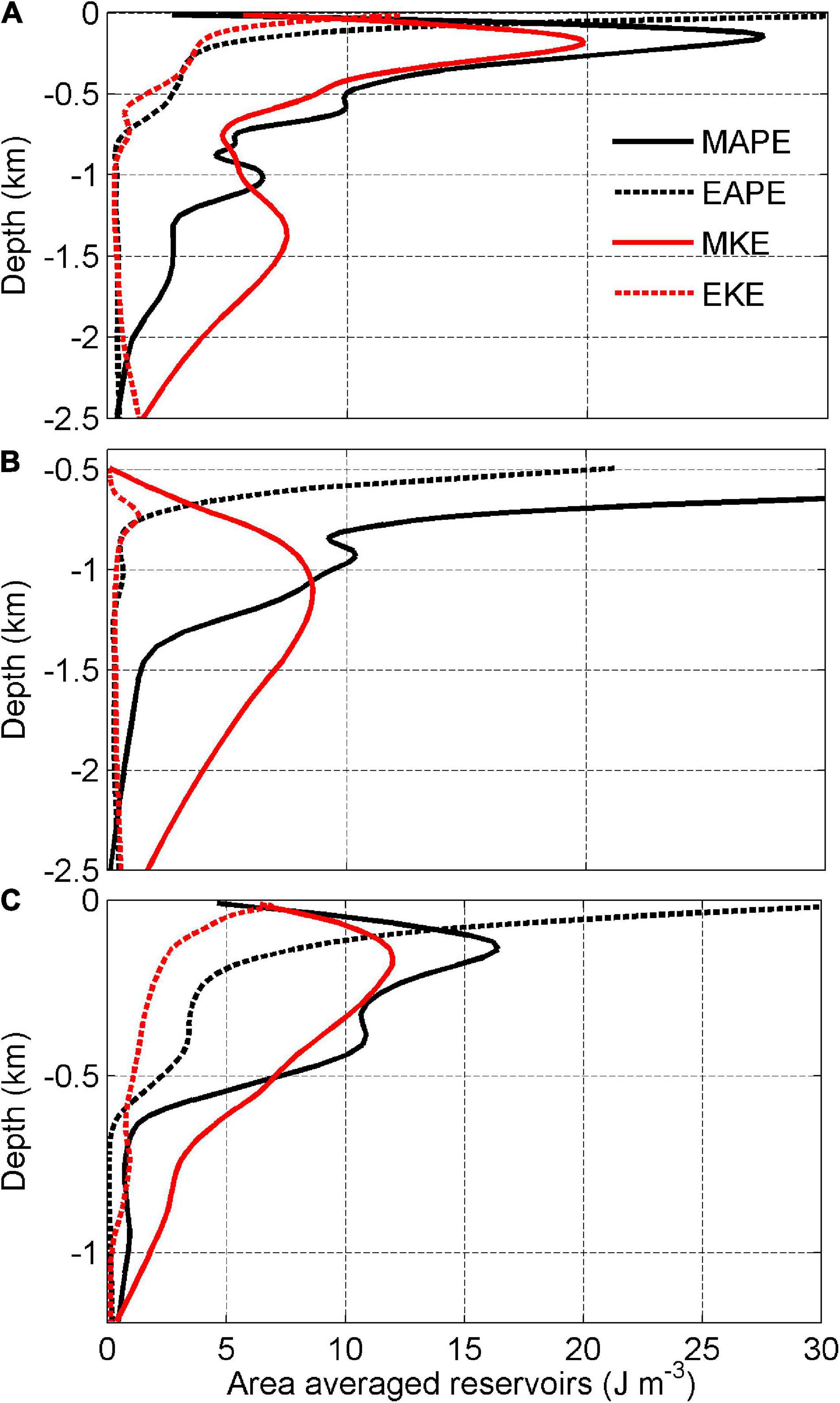
Figure 5. Vertical profiles of area average MAPE (J m^–3), EAPE (J m^–3), MKE (J m^–3), and EKE (J m^–3) over the whole AIS cavity (A), region AIS1 (B), and region AIS2 (C).

Furthermore, the vertical profiles of the four reservoirs are separated into regions AIS1 and AIS2 (Figures 5B,C). In region AIS1, the MKE profile is different from that of MAPE in such a way that the values of MKE increase gradually from 500 to 1,000 m and decrease slightly from 1,000 m to the bottom (Figure 5B). The vertical profiles of MAPE and EAPE in region AIS1 have similar patterns featured by the larger values rapidly decreasing in the upper 800 m. The averaged value of EKE is much smaller than the other reservoirs in region AIS1 with larger values in the depth from 600 to 800 m (Figure 5B). The profiles of energy components in region AIS2 are similar to those over the whole AIS cavity, featured by large values concentrating in the upper 200 m and a large decrease below (Figure 5C).

Generation of APE and Dissipation of KE

Generation of APE

As revealed by Herraiz-Borreguero et al. (2015, 2016a), the modified CDW intrusions are found at the eastern flank of the AIS calving front in the early austral winter. The ice shelf base melting/freezing rate is determined by the temperature difference between the seawater contacting with the ice shelf and the in situ freezing point. Generally, freezing occurs along the west and north of the AIS, and melting occupies the east and south of the AIS, consistent with previous studies (Galton-Fenzi et al., 2012; Depoorter et al., 2013; Rignot et al., 2013; Herraiz-Borreguero et al., 2015). The simulated net basal melt rate is relatively larger than previous modeling studies and observations (Hellmer and Jacobs, 1992; Galton-Fenzi et al., 2012; Depoorter et al., 2013; Rignot et al., 2013), and it might be due to the absence of a frazil ice parameterization in our model (Galton-Fenzi et al., 2012; Herraiz-Borreguero et al., 2013) and the relatively thick vertical layers at the base of the ice shelf in our simulation (Schodlok et al., 2016). The southernmost ISW is formed by the mixing of the inflow water with ice shelf melt water. The maximal melt rate amounts to 30 m yr^–1 at the grounding line. The high melt rate at the grounding line agrees with estimations from previous studies (Wen et al., 2007; Galton-Fenzi et al., 2012). In the western flank of the ocean cavity, ISW ascends along the AIS base and gradually becomes super cooled (cooler than the in situ freezing point temperature), leading to areas of re-freezing (Figures 6A,B). Note that the generation of APE is the total effect including the ice shelf melting and the seawater re-freezing.

FIGURE 6

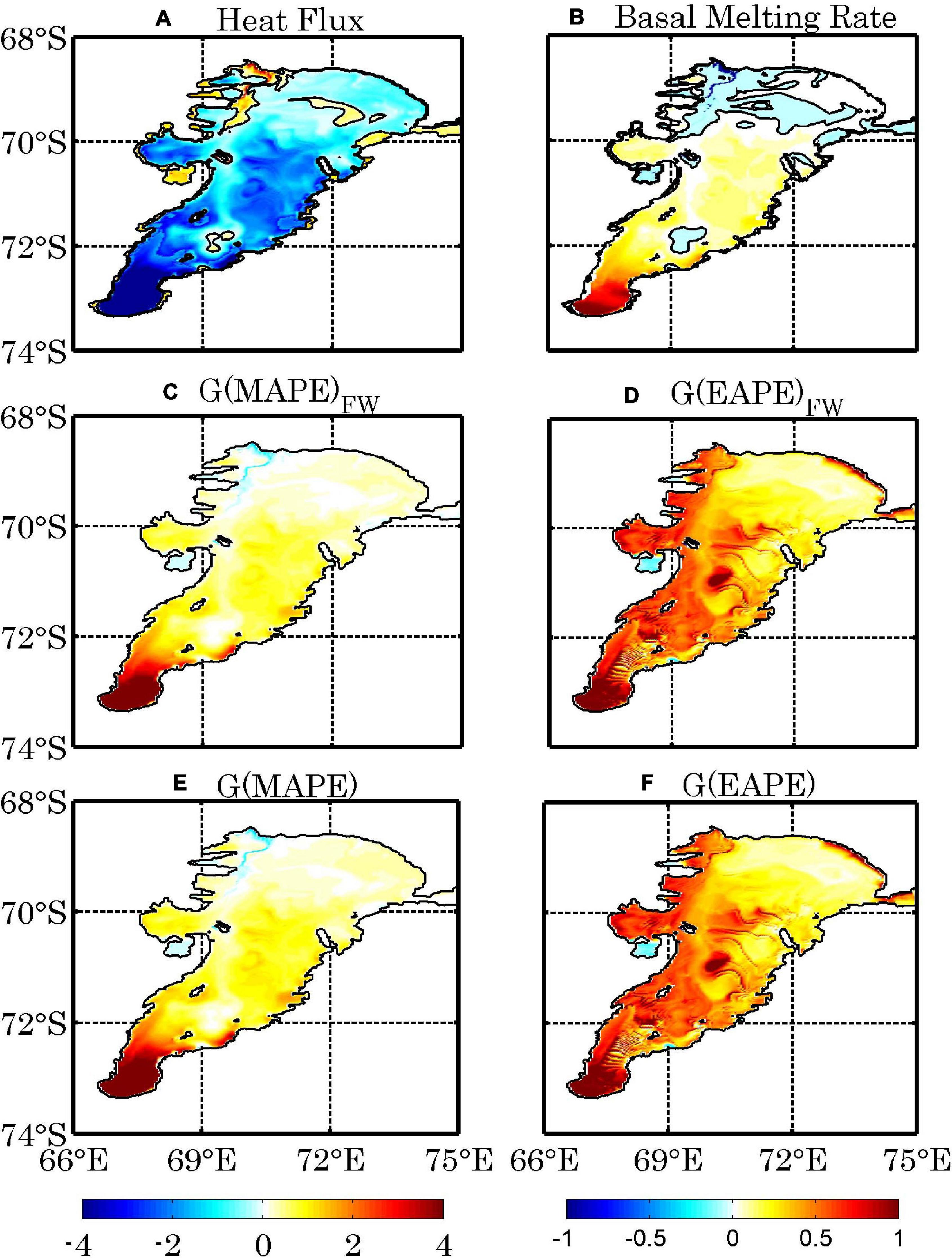
Figure 6. The annual mean net heat flux (1 × 10 W m^–2) (A) and basal melting rate (1 × 10 m yr^–1) (B), the generation rates induced by the freshwater flux for MAPE (1 × 10^–2 W m^–2) (C) and EAPE (1 × 10^–5 W m^–2) (D) at the ice shelf-ocean interface. (E,F) Are the generation rates induced by the total buoyancy flux for MAPE (1 × 10^–2 W m^–2) and EAPE (1 × 10^–5 W m^–2), respectively.

Figures 6E,F show the distributions of the MAPE and EAPE generated by total buoyancy flux, respectively. The pattern of MAPE generation is similar to that of freshwater flux at the ocean-ice shelf interface. Similarly, the pattern of EAPE generation features larger values near the grounding line, and spreads much more evenly over region AIS1. As expected, the APE generation is dominated by the freshwater flux, as salinity is a dominant factor in determining the potential density of cold seawater with temperature close to the in situ freezing point (Figures 6C,D). These regional patterns of MAPE and EAPE generation are important for driving ocean circulation.

Dissipation of KE

The time-mean ice shelf-ocean drag stress and bottom drag stress are shown in Figures 7A,D, which are estimated using the quadratic bulk formula (Hibler and Bryan, 1987; McPhee, 2008). The spatial distributions of ice shelf-ocean drag stress and bottom drag stress are characterized by large values in the eastern and western edges (Figures 7A,D). These patterns reflect that the stresses are induced by the strong inflow and outflow in the eastern and western flanks. The distributions of energy extracted from the ocean by the time-mean ice shelf-ocean drag stress and the bottom drag stress are very similar to the distributions of time-mean drag stresses (Figures 7B,E), featured by notably negative values near the eastern and western flanks. In addition, the patterns of energy dissipation induced by time-varying drag stress (Figures 7C,F) are similar to the distribution of EKE (Figure 2B). The EKE is significantly suppressed by the stresses both at ice shelf base and the bottom topography. Note that the KE in this model can also be dissipated through interior vertical viscosity and biharmonic viscosity, which varies at each time step. Thus, the dissipation terms of KE (D terms) presented here are just approximations, as the focus of this study is to investigate the important effect of the ice pump mechanism on driving the circulation beneath the AIS.

FIGURE 7

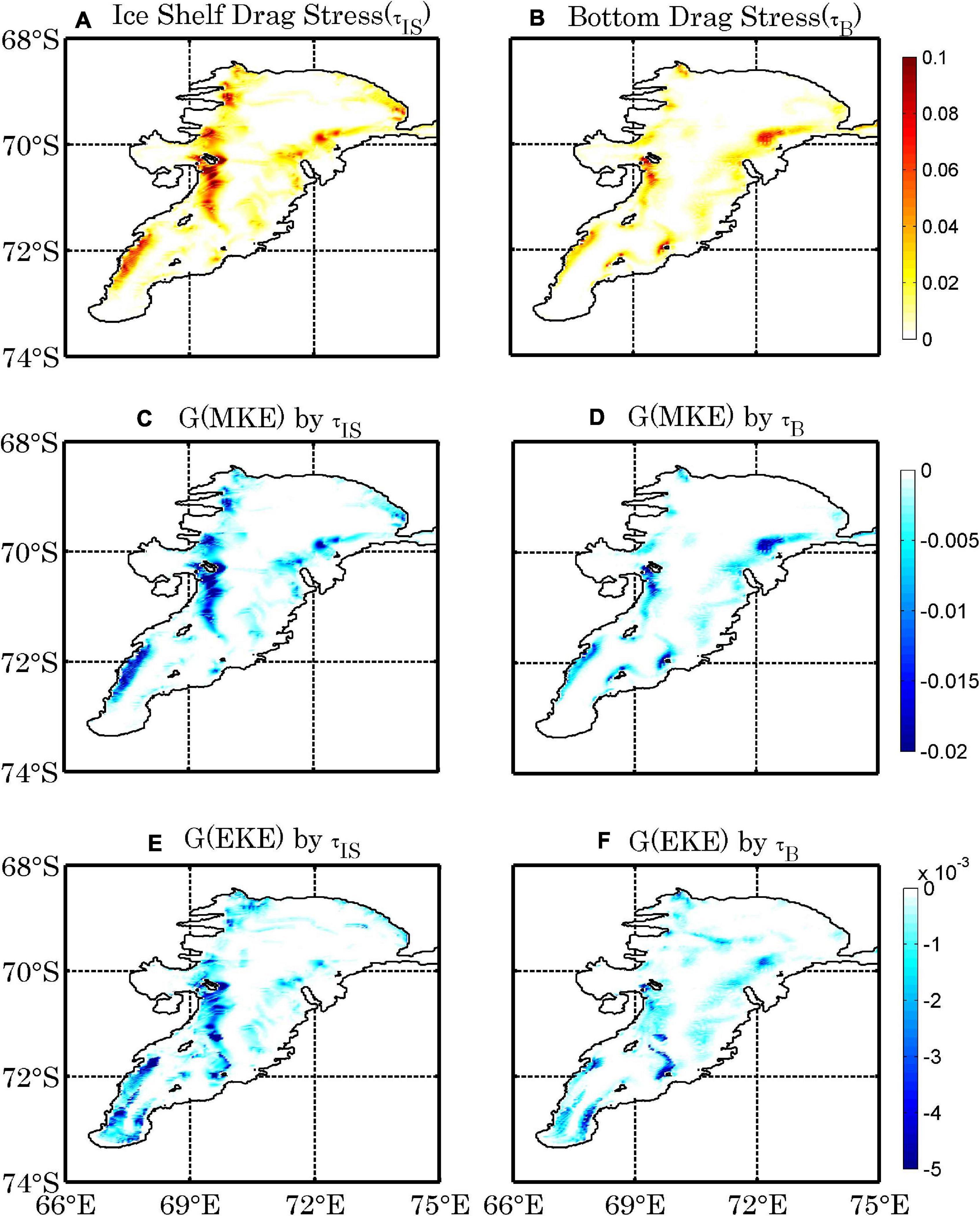
Figure 7. The magnitudes of time-mean drag stress (N m^–2) (A), and the energy dissipations induced by the time-mean (B) and time-varying (C) drag stress at the ice shelf-ocean interface (W m^–2). (D–F) as in (A–C), but for the bottom drag stress and the relevant dissipations.

Energy Conversions

According to equation (10), MAPE is converted into EAPE when the eddy density flux ${}_{\overline{{\mathrm{\rho }}^{\prime }{u}_h^{\prime }}}$ is directed down the mean density gradient. Figure 8A presents the vertically integrated distribution of the conversion from MAPE to EAPE. A positive value indicates energy being transferred from MAPE to EAPE, and a negative value indicates transfer from EAPE to MAPE. The distribution is featured by large positive values concentrated in the western flank of the ocean cavity and in the eastern flank from 69 S to the calving front, while some negative values exist in the central region of AIS2. Similarly, the vertically integrated distribution of energy conversion between EAPE and EKE is characterized by the relatively small positive values across the majority of the AIS cavity and large positive values toward the grounding line (Figure 8B). These results indicate that substantial eddy activities are generated in the AIS1 and the western boundary current in the AIS cavity. In region AIS1, the spatial pattern of energy conversion from EAPE to EKE is featured with mixed positive and negative values. The excess buoyancy obtained through the interactions between the ocean and ice shelf is released by the baroclinic instability, as the buoyant water ascends along the upward-sloping base of the ice shelf. The energy conversions between MAPE, EAPE and EKE indicate a baroclinic pathway in the AIS cavity, which is especially visible in AIS1 and western boundary current regions.

FIGURE 8

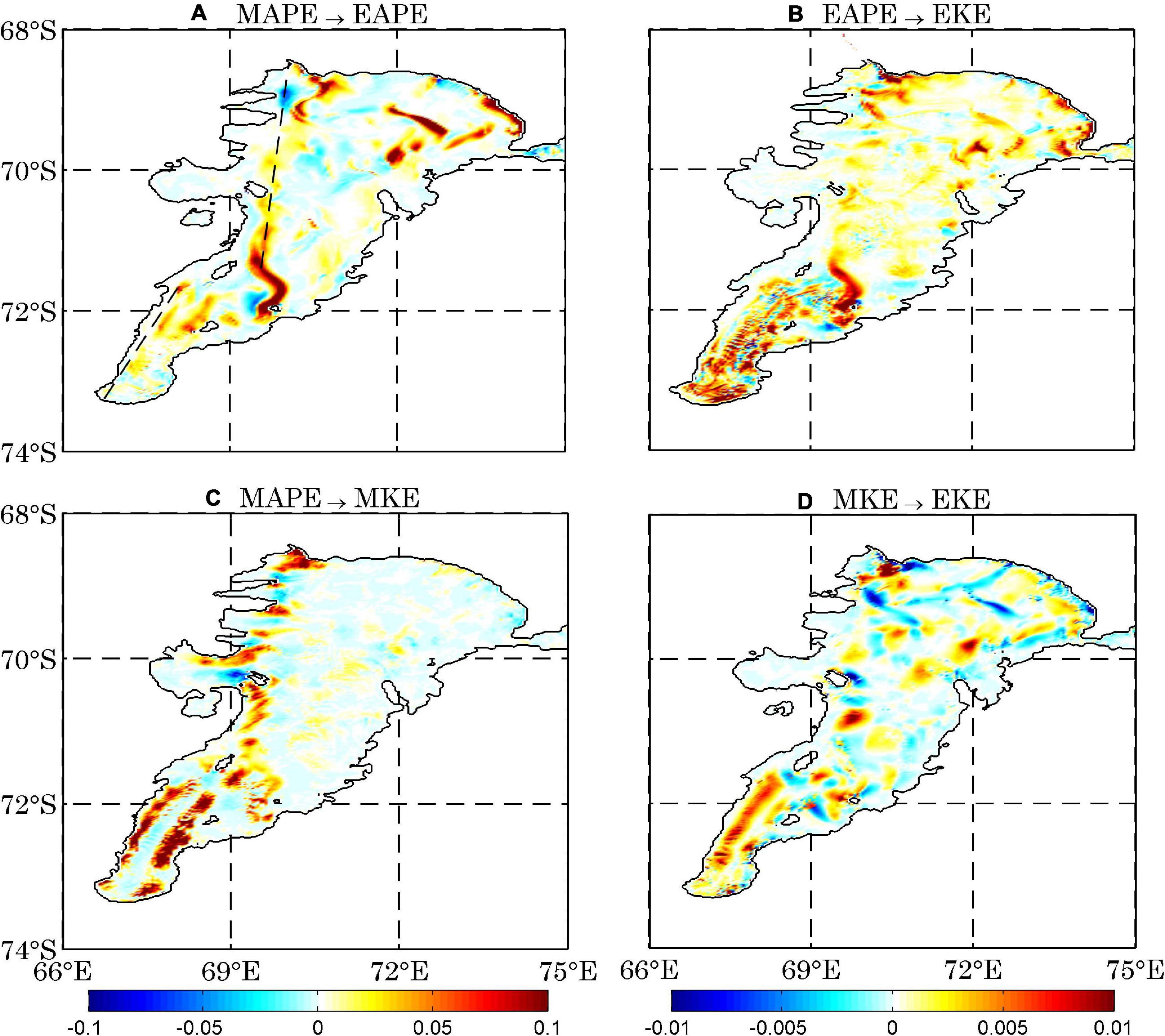
Figure 8. The annual mean distributions of vertically integrated conversion rates between MAPE and EAPE (1 × 10^–1 W m^–2) (A), EAPE and EKE (W m^–2) (B), MAPE and MKE (W m^–2) (C), and MKE and EKE (W m^–2) (D). The positive (negative) value means energy is transferred from MAPE to EAPE (EAPE to MAPE).

Figure 8C gives the vertically integrated distribution of energy conversion between MAPE and MKE, featured by mixed large positive and negative values along the western flank of the AIS cavity in region AIS2 and large positive values in region AIS1, and similar to that between EAPE and EKE (Figure 8B). The large MAPE generation rate in region AIS1 (Figure 6C) is generally balanced by the large conversion rate from MAPE to MKE (Figure 8C), leading to very small MAPE there (Figure 2C). In contrast to the patterns of energy conversions between MAPE, EAPE, and EKE, the energy conversion between MKE and EKE is characterized by mixed positive and negative values over region AIS2 (Figure 8D). However, in region AIS1, the energy is mainly transferred from MKE to EKE especially in the west flank of region AIS1. The energy conversions from MAPE to MKE and then to EKE indicates a different energy conversion pathway rather than the baroclinic one, which is particularly strong over region AIS1. The large energy conversion rate from MAPE to MKE generates much stronger and wider mean current concentrated in the western and eastern boundary regions of AIS1 and western boundary region of AIS2 which is strikingly different from the open ocean. However, the spread and strength of mean current in the open ocean are much narrower and weaker than those of eddy activities (von Storch et al., 2012; Wu et al., 2017a). In the AIS cavity, the buoyancy forcing (i.e., ice pump) is major factor driving the circulation. Hence, the significant positive energy conversion rate from MAPE to MKE is confined in the western AIS cavity (Figur 1). As APE is the only generating source of eddy activity, the energy conversion rate from EAPE to EKE is positive under most of the shelf. The heterogenous pattern of energy conversion rate from MKE to EKE is induced by the interaction between the ocean circulation and the topography as shown in previous studies (Kang and Curchitser, 2015, 2016; Wu et al., 2017a).

Figure 9 presents the vertical distributions of energy conversion rates between the four energy reservoirs. The vertical pattern of the energy conversion between MAPE and EAPE (Figure 9A) is similar to that of the energy conversion between EAPE and EKE (Figure 9B), featured by large values near the interface between the ice shelf and the ocean, especially in region AIS1 (Figures 9A,B). The vertical structure of the energy conversion from MAPE to MKE shows a pattern of large positive values in the upper water column and large negative values in the lower water column from 72 to 73 S (Figure 9C). These large negative values indicate that the MAPE extracts energy from the mean current in the lower water column, similar to the pathway of energy conversion in open ocean. The lower density water from ice shelf melting leads to a more tilted isopycnal surface. Consequently, the energy is transferred from MKE to MAPE in the lower water column. This suggests that stronger currents arise from here than in other areas of the AIS cavity. The vertical distribution of energy conversion rate between MKE and EKE (Figure 9D) is much more homogeneous. In region AIS1, the conversion rate from MKE to EKE is largely positive in the entire water column, except for some negative values close to the ice shelf base (Figure 9D). The positive values mean that the eddy activity is generated by the shear instability there. In region AIS2, there are mixed large positive and negative values but vertically homogenous (Figure 9D). The positive values indicate that the eddy activity is generated by the mean flow through the shear instability. Negative values mean that eddy activity can also supply energy to the mean flow through the energy inverse cascade, such as by the interaction between the mean flow and the topography (Kang and Curchitser, 2015, 2016; Wu et al., 2017a). For all conversion terms it holds that they are dominated by smaller scale structures of positive and negative values. Consequently, only in an integrated sense can a sign or direction be associated with each of the conversions (von Storch et al., 2012; Wu et al., 2017a).

FIGURE 9

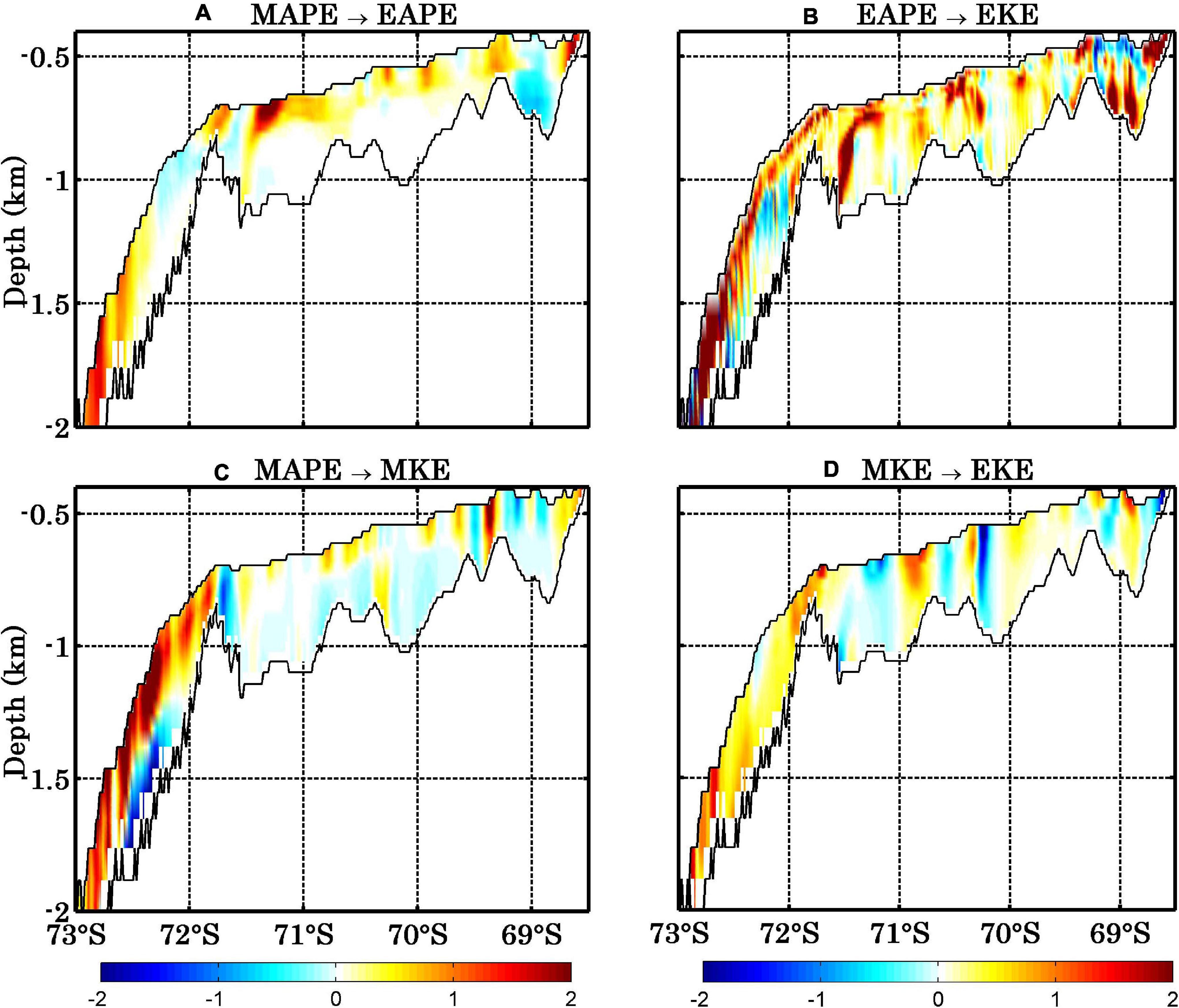
Figure 9. The annual mean vertical distributions of energy conversion rates from MAPE to EAPE (1 × 10^–3 W m^–3) (A), EAPE to EKE (1 × 10^–3 W m^–3) (B), MAPE to MKE (1 × 10^–2 W m^–3) (C), and MKE to EKE (1 × 10^–3 W m^–3) (D), along the sections marked in Figure 9A.

Energy Budget and the Ice Pump Mechanism

Energy Budget

In this section, we present the eddy-mean flow energy budgets integrated over the entire ocean cavity and over two subdomains indicated in Figure 2B. We first examine the energy reservoirs. Over the whole AIS domain, MAPE is the largest energy reservoir (111.6 TJ, 1 TJ = 10¹² J) which is almost two times as large as MKE (70.1 TJ) and more than eleven times larger than EAPE (10.1 TJ). The ratio of EKE to MKE is roughly 8% (Figure 10A), in contrast to that for the Southern Ocean and global ocean, where ratios of EKE to MKE are almost 200 and 280% times, respectively (von Storch et al., 2012; Wu et al., 2017a). However, MKE is the leading energy reservoir in region AIS1 which is 1.4, 8 and 12.2 times as large as MAPE, EAPE, and EKE, respectively. These results indicate a strong conversion of MAPE to MKE and significant suppression of EKE over the whole AIS cavity, especially in region AIS1 (Figures 10A,B). After the much larger MAPE reservoir (63.5 TJ), the MKE reservoir (26.6 TJ) contains much more energy than EAPE and EKE which is roughly 7.8 and 16.7 times as large as EAPE and EKE (Figure 10C) in region AIS2.

FIGURE 10

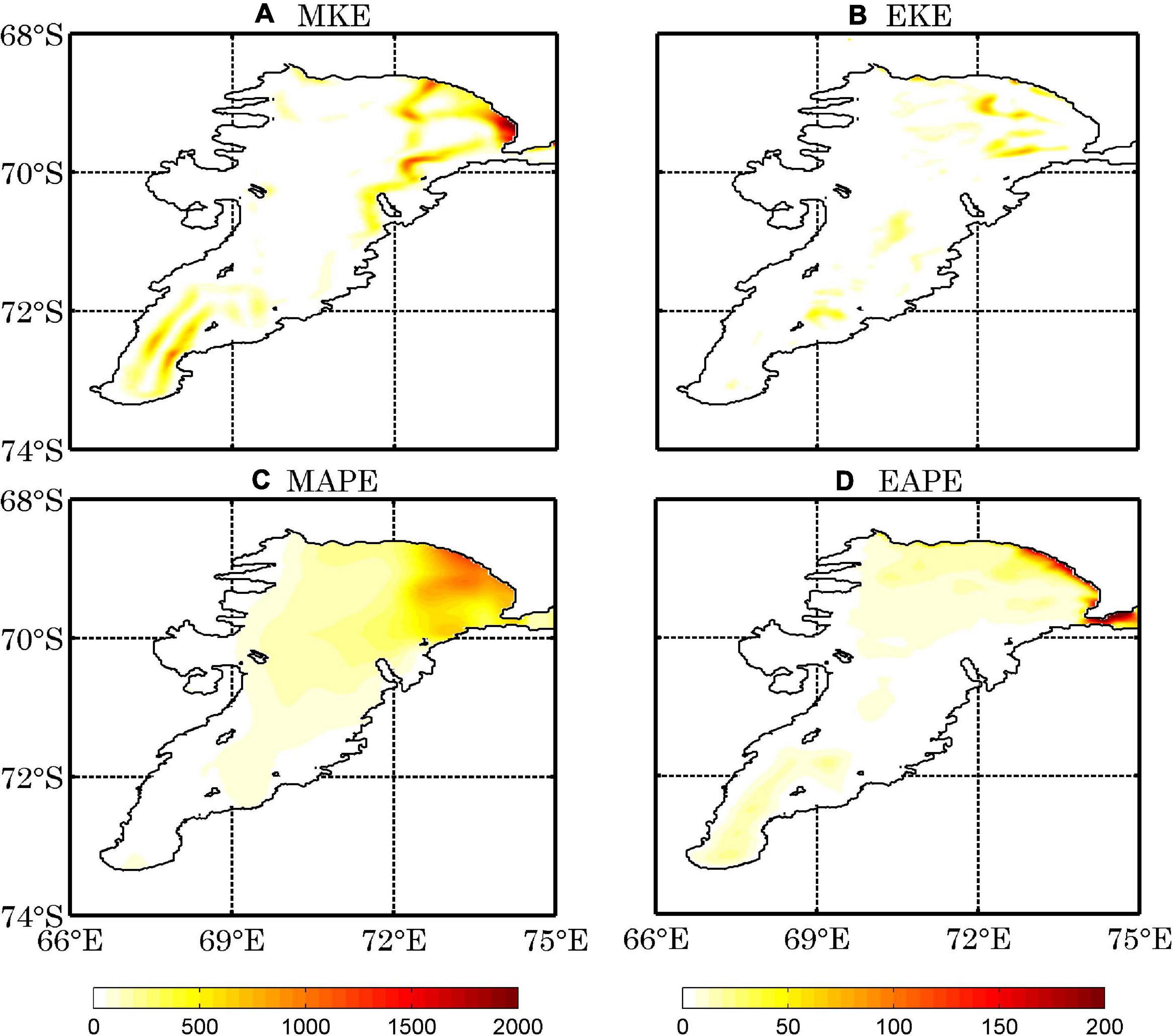
Figure 10. The annual mean distributions of the vertically integrated MKE (A), EKE (B), MAPE (C), and EAPE (D) in the Exp-shutdown experiment (J m^–2).

Integrated over the AIS cavity, the total MAPE generation rate is 0.9 GW (1GW = 10⁹W), dominated by the freshwater forcing with a very small contribution from the heat flux forcing indicating that the thermal contribution to density modification is almost negligible at near freezing point temperature (Figures 6C,E). Similarly, the total EAPE generation rate of 26.9 MW (1MW = 10⁶ W) is composed of a dominant contribution from time-varying freshwater flux (Figure 6D). These results reveal the basal melting is the dominant forcing to drive the current under the AIS cavity. This ice pump generated energy is mainly dissipated by the ice shelf-ocean drag stress and bottom drag stress. The integrated values of _D(MKE) and _D(EKE) induced by ice shelf-ocean drag stress (bottom drag stress) are −0.25 and −0.07 GW (−0.0.15 and −0.03 GW), respectively (Figure 11A).

FIGURE 11

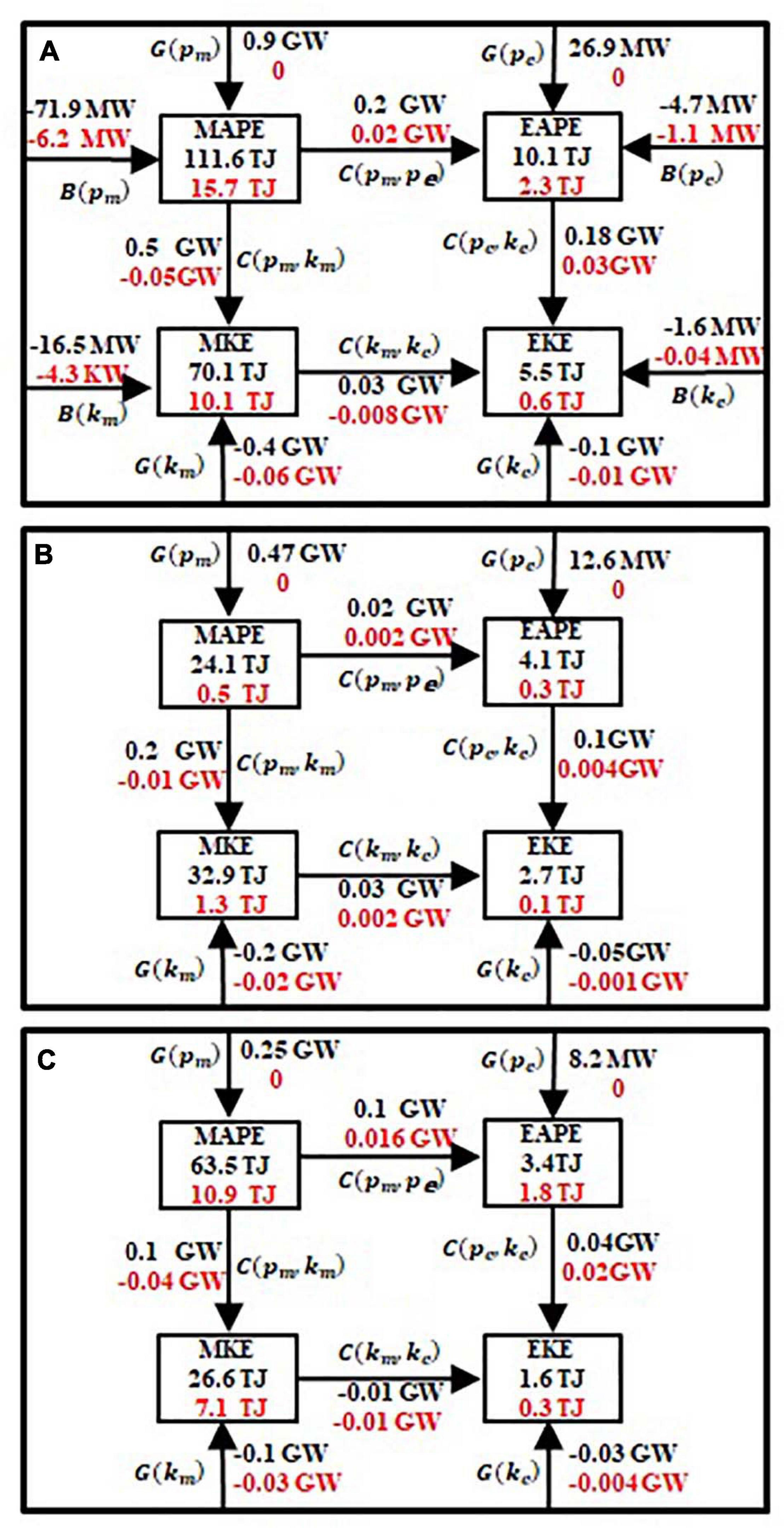
Figure 11. Schematics of energy budgets in the CONTROL (black) and the Exp-shutdown (red) experiments over the whole AIS cavity (A), region AIS1 (B) and region AIS2 (C). The B terms in (A) represent the energy flows through the northern boundary at the AIS calving front.

Regarding the energy conversions among the reservoirs for the entire AIS cavity, the energy is transferred away from the mean flow to the eddy field with an APE conversion rate of 0.2 GW and a KE conversion rate of 0.03 GW. The EKE is generated through two pathways: the barotropic pathway _{MAPE→MKE→EKE}(0.03 GW) and the baroclinic pathway MAPE→EAPE→EKE (0.18 GW), with the baroclinic pathway being dominant. The ratio of barotropic to baroclinic contribution to EKE production is 17%, similar to the ratio for the global ocean, but quite different from the ratio (about 7%) for the Southern Ocean (von Storch et al., 2012; Chen et al., 2014; Wu et al., 2017a). In addition, the MAPE reservoir also supplies 0.5 GW of energy to MKE and facilitates the barotropic pathway (Figure 11A). Region AIS1 has the same energy conversion pathway as the whole AIS cavity, showing two major energy transferring pathways from MAPE: MAPE→EAPE→EKE and MAPE→MKE→EKE with conversion rates of 0.1 GW and 0.03 GW to the EKE, respectively (Figure 11B). In region AIS2, despite the baroclinic pathway having a rate of 0.04 GW, no energy is transferred from MKE to EKE; instead, there is a weak energy transfer from EKE to MKE (Figure 11C). These results indicate that the eddies, on average, are mainly generated in region AIS1, and then act to accelerate the mean flow slightly in region AIS2. The energy flows at the AIS calving front are significantly weaker than the energy conversion rates in the AIS cavity. The circulation in the AIS cavity slightly loses APE and KE at the coastal-portion of the AIS (Figure 11A). The generation of EKE is dominated by the baroclinic pathway, which is driven by the buoyancy input of basal melting in the AIS cavity. This is evidence that general circulation models need to include ice/ocean interaction, with full descriptions of cavity dynamics, to fully measure the energy budgets of the ocean.

The Ice Pump Mechanism

Unlike the open-ocean circulation driven by the atmospheric forcing, the circulation beneath the AIS is mainly driven by the buoyancy power input supplied by the ice shelf basal melting i.e., the ice pump mechanism (Foldvik and Kvinge, 1974; Lewis, 1985; Schodlok et al., 2016). To quantify the impact of ice pump mechanism on the LEC for the circulation in the AIS cavity, we conducted a sensitivity experiment in which the heat and freshwater fluxes at the ice shelf-ocean interface are set to zero. When the buoyancy effects of basal melting and freezing are removed, all the energy reservoirs become very small (Figure 10). The inflow and outflow also become very weak, except for near the eastern calving front (Figure 10), stressing the dominant role of the ice pump mechanism in regulating the cyclonic circulations beneath the ice shelf. The integrated values of the four energy reservoirs, energy conversions and dissipations are also summarized in Figure 11. Again, these results present the dominate role of basal melting in driving the circulation in the AIS cavity. Note that the energy reservoirs in the eastern part of AIS2 are induced by the intrusion of the ocean circulation, and the values of MKE and EAPE in the deepest regions of the ice shelf cavity are probably from the model initial condition. If the model runs for an enough long time, these energy reservoirs will be dissipated.

Concluding Remarks and Discussion

In this study, we conducted a detailed energetic analysis for the circulation in the sub-ice-shelf cavity of the AIS, by using the daily outputs of a high-resolution coupled regional ocean-sea ice-ice shelf model. We examined the characteristics of the four energy components, their generations, dissipations and conversions in the AIS cavity. In particular, the critical role of the ice pump mechanism in driving the energy cycle for the ocean circulation beneath the AIS is investigated quantitatively. By analyzing the model outputs, we obtained the following results:

• The MKE shows a distinct spatial pattern, with the most energetic motions being concentrated in the eastern and western flanks of the AIS cavity, while the EKE is more smoothly spread. The total EKE (5.5 TJ) is just 8% of the MKE (70.1 TJ), indicating a visible suppression of eddy by the stresses of ice shelf and bottom topography in the AIS cavity, which is different from the results for the Southern Ocean and global ocean where the EKE is much larger than MKE. The total EAPE (10.1 TJ) is about 2 times larger than the total EKE.

• The total generation rate of APE amounts to 1.0 GW, almost all of which is generated by the ice pump mechanism. This ice pump generated energy is mainly dissipated by the ice shelf-ocean drag stress and bottom drag stress, amounting to 0.32 and 0.18 GW, respectively.

• The energy is transferred away from MAPE by two pathways: the barotropic pathway MAPE→MKE→EKE and the baroclinic pathway MAPE→EAPE→EKE. The conversion rates from MAPE to MKE and EAPE are 0.5 and 0.2 GW, respectively. In the inner region near the grounding line, the energy pathway is the same as that in the entire AIS region, while in the outer region near the calving front, the eddies act to accelerate the mean flow slightly.

• EKE is mainly generated by baroclinic instability, with 0.18 GW being converted into the EKE from the EAPE, while the barotropic pathway is rather weak, with only 0.03 GW being converted into the EKE from MKE.

These model results elucidated the dynamic processes of eddy generation in the AIS, which differs but complements the results from the recent observational and modeling studies on the AIS and other ice shelves (Galton-Fenzi et al., 2012; Depoorter et al., 2013; Herraiz-Borreguero et al., 2013; Rignot et al., 2013; Schodlok et al., 2016; Liu et al., 2017; Mack et al., 2019). Furthermore, we explored the underlying physical processes quantitatively and gave a description of dynamics in AIS cavity. The distinct characteristics of the energy cycle in the AIS cavity are revealed. The results obtained in this study offer useful benchmarks for analyzing energy cycles in other sub-ice-shelf cavities and provide a more complete understanding of the ocean dynamics in the sub-ice-shelf cavities. The potential energy is stored in the titled isopycnal surfaces and it is increased by adding buoyancy from lighter water masses or by extracting buoyancy from denser water masses. Likewise, potential energy is decreasing by extracting buoyancy from lighter water masses or by adding buoyancy to denser water masses. The ice shelf basal melting supplies most potential energy in the AIS cavity by influencing the sea water density. The density of sea water in the ice shelf cavity is strongly influenced by buoyancy flux through heat and freshwater exchanges between ice shelf and sea water. The relaxation of isopycnal surfaces is mainly through the processes associated with topography features (Wu et al., 2017a). The released energy is used to generate eddy activities. This energy pathway is usually named baroclinic pathway which is the dominated one to generate eddy activity. The other energy pathway of eddy activity generation is named barotropic pathway that MKE supplies energy to the eddy activity by the shear instability. The patterns of energy conversion terms are dominated by smaller scale structures of positive and negative values. Consequently, an integrated sense is needed to find the energy conversion pathway. The ice shelf base and bottom topography both dissipate the kinetic energy of ocean circulation in the ice shelf cavity. Hence, the eddy activities are suppressed significantly in the ice shelf cavity. This is different from the open ocean where the wind can supply energy to the eddy activity.

We acknowledge that this study has some limitations. Firstly, the definition of APE is an approximation, especially in the high-latitude deep convection regions (Zemskova et al., 2015). Secondly, there are several numerical model limitations, such as the uncertain geometry of the sub-ice-shelf cavity (Galton-Fenzi et al., 2012), the uncertain treatments of heat and freshwater exchanges at the interface of ocean-ice shelf, and the coarse model resolution which cannot fully capture the eddy activity in the cavity, especially in destratified water column as commonly observed in polar winter conditions and under cold ice shelves it can become very small < 1 km (Nurser and Bacon, 2014; Mack et al., 2019). For example, Mack et al. (2019) calculated a mean deformation radius for on-shelf winter conditions in the Ross Sea of 1.7 km. They noted a resolution of 350 m or less would be required to capture 95% of the eddy activity especially in the cavity. However, it is not computationally feasible at this time (Mack et al., 2019). Lastly, our model does not include a frazil ice parameterization.

It is also noted that the frazil-ice formation process was found important in determining the basal melting/freezing rate of the AIS (Galton-Fenzi et al., 2012; Herraiz-Borreguero et al., 2013). The frazil ice formation can lead to increased salinity, and hence moderate the circulation pattern and the maximum amount of super-cooling beneath the ice shelf. The frazil crystals can also input more buoyancy to the ocean to accelerate the current under the AIS (Jenkins and Bombosch, 1995). The lack of this process leads to a decrease of marine ice formation (Galton-Fenzi et al., 2012; Herraiz-Borreguero et al., 2013; Hughes et al., 2014), influences the ISW outflow properties (Jordan et al., 2015). Our model also does not include the tidal forcing which is important in modulating the ice shelf basal melting and altering the thermohaline circulation in the sub-ice-shelf cavity by pumping warm water into the sub-ice-shelf cavity and increasing the friction at the ice water interface (Holland and Jenkins, 1999; Padman et al., 2003; Robertson, 2013; Jendersie et al., 2018). Hence, the lack of tidal forcing leads to a decrease of the basal melting and the energy dissipation, and hence influences the whole energy cycle in the AIS cavity. Additionally, the radar surveys and in situ measurements revealed a mass of sinuous subglacial channels typically 500 m to 3 km wide, and up to 200 m high, in the ice-shelf base (Vaughan et al., 2012; Stanton et al., 2013). These channels in the ice shelf base enhance the ice shelf basal melting of Pine Island Glacier as large as 0.06 m/day at the channel apex (Stanton et al., 2013). While large channels in the AIS base were found many decades ago (Mellor and McKinnon, 1960), the impact of channels on AIS basal melting has not been investigated. The channels would enhance the AIS basal melting and then lead to a much more buoyant melt water and increased the APE of the circulation under the ice shelf cavity, and therefore strengthen the whole energy cycle. In addition, the presence of these channels are likely to contribute to significant form drag that will increase the ocean/ice drag coefficient in the cavity part of the model domain, and strengthen mesoscale eddy dissipation rates.

Future studies should thus be devoted to the following aspects. Firstly, an understanding of the impacts of frazil ice processes on the energy pathway, and a more complete understanding of the energy cycle in a sub-ice-shelf cavity is needed. Secondly, the effects of tidal forcing on the energy pathway in the ice shelf cavity need systematic study. Thirdly, the 3-D structure of mesoscale eddy and the energetics of the eddy activity during its whole life cycle within the ice shelf cavity need detailed investigation. Additionally, the detailed study of the seasonal variability of energy budget in the AIS cavity is underway.

Data Availability Statement

The data used to reproduce these figures in this manuscript can be found below: https://pan.baidu.com/s/1T4pLmvCb5bLG7mw5_iGBXw (code: 1234). The model outputs used in this study are available upon request (yang.wu@njxzc.edu.cn).

Author Contributions

YW performed the methodology, ran the numerical model, data analyses, and wrote the original manuscript draft. YW, ZW, CL, and LY participated in the manuscript revision and improvement. All authors contributed to the article and approved the submitted version.

Funding

This study was supported by the National Natural Science Foundation of China (Grant Nos. 41941007, 41806216, and 41876220), the China Postdoctoral Science Foundation (Grant Nos. 2019T120379 and 2018M630499), and the Talent start-up fund of Nanjing Xiaozhuang University (Grant No. 4172111).

Conflict of Interest

The authors declare that the research was conducted in the absence of any commercial or financial relationships that could be construed as a potential conflict of interest.

Acknowledgments

The MITgcm code was obtained freely from http://mitgcm.org/. The atmospheric forcing data were obtained freely from the NCAR’s research data archive (JRA-55: https://rda.ucar.edu/datasets/ds625.0/). We thank the editor and two reviewers for their positive and constructive comments and suggestions.

References

Chen, R., Flierl, G. R., and Wunsch, C. (2014). A description of local and nonlocal eddy-mean flow interaction in a global eddy-permitting state estimate. J. Phys. Oceanogr. 44, 2336–2352. doi: 10.1175/jpo-d-14-0009.1

CrossRef Full Text | Google Scholar

Couto, N., Martinson, D. G., Kohut, J., and Schofield, O. (2017). Distribution of upper circumpolar deep water on the warming continental shelf of the West Antarctic Peninsula. J. Geophys. Res. 119, 5306–5315.

Google Scholar

Cox, M. D. (1985). An eddy resolving model of the ventilated thermocline. J. Phys. Oceanogr. 15, 1312–1324. doi: 10.1175/1520-0485(1985)015<1312:aernmo>2.0.co;2

CrossRef Full Text | Google Scholar

Dansereau, V., Heimbach, P., and Losch, M. (2014). Simulation of subice shelf melt rates in a general circulation model: velocity-dependent transfer and the role of friction. J. Geophys. Res. 119, 1765–1790. doi: 10.1002/2013jc008846

CrossRef Full Text | Google Scholar

Depoorter, M. A., Bamber, J. L., Griggs, J. A., Lenaerts, J. T. M., Ligtenberg, S. R. M., van den Broeke, M. R., et al. (2013). Calving fluxes and basal melt rates of Antarctic ice shelves. Nature 502, 89–92. doi: 10.1038/nature12567

PubMed Abstract | CrossRef Full Text | Google Scholar

Dinniman, M. S., Klinck, J. M., Bai, L. S., Bromwich, D. H., Hines, K. M., and Holland, D. M. (2015). The effect of atmospheric forcing resolution on delivery of ocean heat to the Antarctic floating ice shelves. J. Clim. 28, 6067–6085. doi: 10.1175/jcli-d-14-00374.1

CrossRef Full Text | Google Scholar

Eden, C., and Boning, C. (2002). Sources of eddy kinetic energy in the Labrador Sea. J. Phys. Oceanogr. 2, 3346–3363. doi: 10.1175/1520-0485(2002)032<3346:soekei>2.0.co;2

CrossRef Full Text | Google Scholar

Foldvik, A., and Kvinge, T. (1974). Conditional instability of sea-water at freezing-point. Deep Sea Res. 21, 169–174. doi: 10.1016/0011-7471(74)90056-4

CrossRef Full Text | Google Scholar

Fricker, H. A., Hyland, G., Coleman, R., and Young, N. W. (2000). Digital elevation models for the Lambert Glacier-Amery Ice Shelf system, East Antarctica, from ERS-1 satellite radar altimetry. J. Glaciol. 46, 553–560. doi: 10.3189/172756500781832639

CrossRef Full Text | Google Scholar

Galton-Fenzi, B. K., Hunter, J. R., Coleman, R., Marsland, S. J., and Warner, R. C. (2012). Modeling the basal melting and marine ice accretion of the Amery Ice Shelf. J. Geophys. Res. 117, 1–19.

Google Scholar

Graham, J. A., Dinniman, M. S., and Klinck, J. M. (2016). Impact of model resolution for on-shelf heat transport along the West Antarctic Peninsula. J. Geophys. Res. 121, 7880–7897. doi: 10.1002/2016jc011875

CrossRef Full Text | Google Scholar

Griffies, S. M., and Hallberg, R. W. (2000). Biharmonic friction with a Smagorinsky-like viscosity for use in large-scale eddy-permitting ocean models. Mon. Weather Rev. 128, 2935–2946. doi: 10.1175/1520-0493(2000)128<2935:bfwasl>2.0.co;2

CrossRef Full Text | Google Scholar

Hallberg, R. (2013). Using a resolution function to regulate parameterizations of oceanic mesoscale eddy effects. Ocean Model. 72, 92–103. doi: 10.1016/j.ocemod.2013.08.007

CrossRef Full Text | Google Scholar

Hattermann, T., Smedsrud, L. H., Nøst, O. A., Lilly, J. M., and Galton-Fenzi, B. K. (2014). Eddy-resolving simulations of the Fimbul Ice Shelf cavity circulation: basal melting and exchange with open ocean. Ocean Model. 82, 28–44. doi: 10.1016/j.ocemod.2014.07.004

CrossRef Full Text | Google Scholar

Heil, P., Allison, I., and Lytle, V. I. (1996). Seasonal and interannual variations of the oceanic heat flux under a land fast Antarctic sea ice cover. J. Geophys. Res. 101, 25741–25752. doi: 10.1029/96jc01921

CrossRef Full Text | Google Scholar

Hellmer, H. H., and Jacobs, S. S. (1992). Ocean interactions with the base of the Amery Ice Shelf, Antarctica. J. Geophys. Res. 97, 20305–20317. doi: 10.1029/92jc01856

CrossRef Full Text | Google Scholar

Hellmer, H. H., and Olbers, D. J. (1989). A two-dimensional model of the thermohaline circulation under an ice shelf. Antarct. Sci. 1, 325–336. doi: 10.1017/s0954102089000490

CrossRef Full Text | Google Scholar

Hemer, M. A., Hunter, J. R., and Coleman, R. (2006). Barotropic tides beneath the Amery Ice Shelf. J. Geophys. Res. 111, 1–13.

Google Scholar

Herraiz-Borreguero, L., Allison, I., Craven, M., Nicholls, K. W., and Rosenberg, M. A. (2013). Ice shelf/ocean interactions under the Amery Ice Shelf: seasonal variability and its effect on marine ice formation. J. Geophys. Res. Oceans 118, 7117–7131. doi: 10.1002/2013jc009158

CrossRef Full Text | Google Scholar

Herraiz-Borreguero, L., Church, J. A., Allison, I., Peña-Molino, B., Coleman, R., Tomczak, M., et al. (2016a). Basal melt, seasonal water mass transformation, ocean current variability, and deep convection processes along the Amery Ice Shelf calving front, East Antarctica. J. Geophys. Res. Oceans 121, 4946–4965. doi: 10.1002/2016jc011858

CrossRef Full Text | Google Scholar

Herraiz-Borreguero, L., Coleman, R., Allison, I., Rintoul, S. R., Craven, M., and Williams, G. D. (2015). Circulation of modified circumpolar deep water and basal melt beneath the Amery Ice Shelf, East Antarctica. J. Geophys. Res. Oceans 120, 3098–3112. doi: 10.1002/2015jc010697

CrossRef Full Text | Google Scholar

Herraiz-Borreguero, L., Lannuzel, D., van der Merwe, P., Treverrow, A., and Pedro, J. B. (2016b). Large flux of iron from the Amery Ice Shelf marine ice to Prydz Bay, East Antarctica. J. Geophys. Res. Oceans 121, 6009–6020. doi: 10.1002/2016jc011687

CrossRef Full Text | Google Scholar

Hibler, W. D., and Bryan, K. (1987). A diagnostic ice-ocean model. J. Phys. Oceanogr. 17, 987–1015. doi: 10.1175/1520-0485(1987)017<0987:adim>2.0.co;2

CrossRef Full Text | Google Scholar

Holland, D. M., and Jenkins, A. (1999). Modeling thermodynamic ice-ocean interactions at the base of an ice shelf. J. Phys. Oceanogr. 29, 1787–1800. doi: 10.1175/1520-0485(1999)029<1787:mtioia>2.0.co;2

CrossRef Full Text | Google Scholar

Huang, R. X. (2005). Available potential energy in the world’s oceans. J. Mar. Res. 63, 141–158. doi: 10.1357/0022240053693770

CrossRef Full Text | Google Scholar

Huang, R. X., Wang, W., and Liu, L. L. (2006). Decadal variability of wind-energy input to the world ocean. Deep Sea Res. II Top. Stud. Oceanogr. 53, 31–41. doi: 10.1016/j.dsr2.2005.11.001

CrossRef Full Text | Google Scholar

Hughes, C. W., and Wilson, C. (2008). Wind work on the geostrophic ocean circulation: an observational study on the effect of small scales in the wind stress. J. Geophys. Res. 113, 1–10.

Google Scholar

Hughes, K. G., Langhorne, P. J., Leonard, G. H., and Stevens, C. L. (2014). Extension of an ice shelf water plume model beneath sea ice with application in McMurdo Sound, Antarctica. J. Geophys. Res. Oceans 119, 8662–8687. doi: 10.1002/2013jc009411

CrossRef Full Text | Google Scholar

Jackett, D. R., and McDougall, T. J. (1995). Minimal adjustment of hydrostatic profiles to achieve static stability. J. Atmos. Ocean. Technol. 12, 381–389. doi: 10.1175/1520-0426(1995)012<0381:maohpt>2.0.co;2

CrossRef Full Text | Google Scholar

Jendersie, S., Williams, M., Langhorne, P. J., and Robertson, R. (2018). The density-driven winter intensification of the Ross Sea circulation. J. Geophys. Res. 123, 7702–7724. doi: 10.1029/2018jc013965

CrossRef Full Text | Google Scholar

Jenkins, A., and Bombosch, A. (1995). Modelling the effects of frazil ice crystals on the dynamics and thermodynamics of ice shelf water plumes. J. Geophys. Res. 100, 6967–6981. doi: 10.1029/94jc03227

CrossRef Full Text | Google Scholar

Jenkins, A., Hellmer, H. H., and Holland, D. M. (2001). The role of meltwater advection in the formulation of conservative boundary conditions at an ice-ocean interface. J. Phys. Oceanogr. 31, 285–296. doi: 10.1175/1520-0485(2001)031<0285:tromai>2.0.co;2

CrossRef Full Text | Google Scholar

Jordan, J. R., Kimura, S., Holland, P. R., Jenkins, A., and Piggott, M. D. (2015). On the conditional frazil ice instability in seawater. J. Phys. Oceanogr. 45, 1121–1138. doi: 10.1175/jpo-d-14-0159.1

CrossRef Full Text | Google Scholar

Joughin, I., and Alley, R. B. (2011). Stability of the West Antarctic ice sheet in a warming world. Nat. Geosci. 4, 506–513. doi: 10.1038/ngeo1194

CrossRef Full Text | Google Scholar

Kang, D. J., and Curchitser, E. N. (2015). Energetics of eddy-mean flow interactions in the Gulf Stream region. J. Phys. Oceanogr. 45, 1103–1120. doi: 10.1175/jpo-d-14-0200.1

CrossRef Full Text | Google Scholar

Kang, D. J., and Curchitser, E. N. (2016). Seasonal variability of the Gulf Stream kinetic energy. J. Phys. Oceanogr. 46, 1189–1207. doi: 10.1175/jpo-d-15-0235.1

CrossRef Full Text | Google Scholar

Kobayashi, S., Ota, Y., Harada, Y., Ebita, A., Moriya, M., Onoda, H., et al. (2015). The JRA-55 reanalysis: general specifications and basic characteristics. J. Meteorol. Soc. Japan 93, 5–48. doi: 10.2151/jmsj.2015-001

PubMed Abstract | CrossRef Full Text | Google Scholar

Large, W., McWilliams, J., and Doney, S. (1994). Oceanic vertical mixing: a review and a model with a nonlocal boundary layer parameterization. Rev. Geophys. 32, 363–403. doi: 10.1029/94rg01872

CrossRef Full Text | Google Scholar

Lewis, E. L. (1985). The “Ice Pump”, A Mechanism for Ice-Shelf Melting, in Glaciers, Ice Sheets, and Sea Level: Effect of a CO₂-Induced Climate Change. Rep. DOE/EV/60235-1. Washington, DC.: U.S. Dep. of Energy, 275–278.

Google Scholar

Liang, X. S., and Robinson, A. R. (2005). Localized multiscale energy and vorticity analysis: I. Fundamentals. Dyn. Atmos. Oceans 38, 195–230. doi: 10.1016/j.dynatmoce.2004.12.004

CrossRef Full Text | Google Scholar

Liang, X. S., and Robinson, A. R. (2007). Localized multi-scale energy and vorticity analysis: II. Finite-amplitude instability theory and validation. Dyn. Atmos. Oceans 44, 51–76. doi: 10.1016/j.dynatmoce.2007.04.001

CrossRef Full Text | Google Scholar

Liu, C., Wang, Z., Cheng, C., Xia, R., Li, B., and Xie, Z. (2017). Modeling modified circumpolar deep water intrusions onto the Prydz Bay continental shelf, East Antarctica. J. Geophys. Res. Oceans 122, 5198–5217.

Google Scholar

Lorenz, E. N. (1955). Available potential energy and the maintenance of the general circulation. Tellus 7, 157–167. doi: 10.1111/j.2153-3490.1955.tb01148.x

CrossRef Full Text | Google Scholar

Losch, M. (2008). Modeling ice shelf cavities in a z coordinate ocean general circulation model. J. Geophys. Res. 113, 1–15.

Google Scholar

Lucarini, V., and Ragone, F. (2011). Energetics of climate models: net energy balance and meridional enthalpy transport. Rev. Geophys. 49, 1–29. doi: 10.1002/9783527698844.ch1

CrossRef Full Text | Google Scholar

Mack, S. L., Dinniman, M. S., Klinck, J. M., McGillicuddy, D. J. Jr., and Padman, L. (2019). Modeling ocean eddies on Antarctica’s cold water continental shelves and their effects on ice shelf basal melting. J. Geophys. Res. Oceans 124, 5067–5084. doi: 10.1029/2018jc014688

CrossRef Full Text | Google Scholar

Maltrud, M. E., Bryan, F. O., and Peacock, S. (2010). Boundary impulse response functions in a century-long global eddying ocean simulation. Environ. Fluid Mech. 10, 275–295. doi: 10.1007/s10652-009-9154-3

CrossRef Full Text | Google Scholar

Marshall, J., Adcroft, A., Hill, C., Perelman, L., and Heisey, C. (1997a). A finite-volume, incompressible Navier Stokes model for studies of the ocean on parallel computers. J. Geophys. Res. 102, 5753–5766. doi: 10.1029/96jc02775

CrossRef Full Text | Google Scholar

Marshall, J., Hill, C., Perelman, L., and Adcroft, A. (1997b). Hydrostatic, quasi-hydrostatic, and nonhydrostatic ocean modeling. J. Geophys. Res. 102, 5733–5752. doi: 10.1029/96jc02776

CrossRef Full Text | Google Scholar

Martinson, D. G., and McKee, D. C. (2012). Transport of warm upper circumpolar deep water onto the Western Antarctic Peninsula continental shelf. Ocean Sci. 8, 433–442. doi: 10.5194/os-8-433-2012

CrossRef Full Text | Google Scholar

McPhee, M. G. (2008). Air-Ice-Ocean Interaction: Turbulent Ocean Boundary Layer Exchange Processes. Berlin: Springer, 1–215.

Google Scholar

Mellor, M., and McKinnon, G. (1960). The Amery Ice Shelf and its hinterland. Polar Rec. 10, 30–34. doi: 10.1017/s0032247400050579

CrossRef Full Text | Google Scholar

Menemenlis, D., Campin, J.-M., Heimbach, P., Hill, C. C., Lee, T., Nguyen, A., et al. (2008). ECCO2: high resolution global ocean and sea ice data synthesis. Mercator Ocean Q. Newslett. 31, 13–21.

Google Scholar

Moffat, C., Owens, B., and Beardsley, R. C. (2009). On the characteristics of circumpolar deep water intrusions to the west Antarctic Peninsula continental shelf. J. Geophys. Res. 114:C05017.

Google Scholar

Mueller, R. D., Hattermann, T., Howard, S. L., and Padman, L. (2018). Tidal inflfluences on a future evolution of the Filchner-Ronne Ice Shelf cavity in the Weddell Sea, Antarctica. Cryosphere 12, 453–476. doi: 10.5194/tc-12-453-2018

CrossRef Full Text | Google Scholar

Nakayama, Y., Timmermann, R., Schröder, M., and Hellmer, H. (2014). On the difficulty of modeling circumpolar deep water intrusions onto the Amundsen Sea continental shelf. Ocean Model. 84, 26–34. doi: 10.1016/j.ocemod.2014.09.007

CrossRef Full Text | Google Scholar

Naughten, K. A., Jenkins, A., Holland, P. R., Mugford, R. I., Nicholls, K. W., and Munday, D. R. (2019). Modeling the Influence of the Weddell Polynya on the Filchner-Ronne Ice Shelf Cavity. J. Clim. 32, 5289–5303. doi: 10.1175/jcli-d-19-0203.1

CrossRef Full Text | Google Scholar

Nunes Vaz, R. A., and Lennon, G. W. (1996). Physical oceanography of the Prydz Bay region of Antarctic waters. Deep Sea Res. I 43, 603–641. doi: 10.1016/0967-0637(96)00028-3

CrossRef Full Text | Google Scholar

Nurser, A. J. G., and Bacon, S. (2014). The Rossby radius in the arctic ocean. Ocean Sci. 10, 967–975. doi: 10.5194/os-10-967-2014

CrossRef Full Text | Google Scholar

Olbers, D., Willebrand, J., and Eden, C. (2012). Ocean Dynamics. Berlin: Springer, 1–199.

Google Scholar

Oort, A., Anderson, L., and Peixoto, J. (1994). Estimates of the energy cycle of the oceans. J. Geophys. Res. 99, 7665–7688. doi: 10.1029/93jc03556

CrossRef Full Text | Google Scholar

Oort, A. H., and Peixoto, J. P. (1983). Global angular momentum and energy balance requirements from observations. Adv. Geophys. 25, 355–490. doi: 10.1016/s0065-2687(08)60177-6

CrossRef Full Text | Google Scholar

Padman, L., Erofeeva, S., and Joughin, I. A. N. (2003). Tides of the Ross Sea and Ross Ice Shelf cavity. Antarct. Sci. 15, 31–40. doi: 10.1017/s0954102003001032

CrossRef Full Text | Google Scholar

Post, A. L., Galton-Fenzi, B. K., Riddle, M. J., Herraiz-Borreguero, L., O’Brien, P. E., Hemer, M. A., et al. (2014). Modern sedimentation, circulation and life beneath the Amery Ice Shelf, East Antarctica. Cont. Shelf Res. 74, 77–87. doi: 10.1016/j.csr.2013.10.010

CrossRef Full Text | Google Scholar

Pritchard, H. D., Ligtenberg, S. R. M., Fricker, H. A., Vaughan, D. G., Van den Broeke, M. R., and Padman, L. (2012). Antarctic ice-sheet loss driven by basal melting of ice shelves. Nature 484, 502–505. doi: 10.1038/nature10968

PubMed Abstract | CrossRef Full Text | Google Scholar

Rignot, E., Jacobs, S., Mouginot, J., and Scheuchl, B. (2013). Ice shelf melting around Antarctica. Science 341, 266–270. doi: 10.1126/science.1235798

PubMed Abstract | CrossRef Full Text | Google Scholar

Robertson, R. (2013). Tidally induced increases in melting of Amundsen Sea ice shelves. J. Geophys. Res. 118, 3138–3145. doi: 10.1002/jgrc.20236

CrossRef Full Text | Google Scholar

Roquet, F., Wunsch, C., and Madec, G. (2011). On the patterns of wind-power input to the ocean circulation. J. Phys. Oceanogr. 41, 2328–2342. doi: 10.1175/jpo-d-11-024.1

CrossRef Full Text | Google Scholar

Roullet, G., Capet, X., and Maze, G. (2014). Global interior eddy available potential energy diagnosed from Argo floats. Geophys. Res. Lett. 41, 1651–1656. doi: 10.1002/2013gl059004

CrossRef Full Text | Google Scholar

Schodlok, M. P., Menemenlis, D., and Rignot, E. J. (2016). Ice shelf basal melt rates around Antarctica from simulations and observations. J. Geophys. Res. Oceans 121, 1085–1109. doi: 10.1002/2015jc011117

CrossRef Full Text | Google Scholar

Scott, R. B., and Xu, Y. (2009). An update on the wind power input to the surface geostrophic flow of the world ocean. Deep Sea Res. I 56, 295–304. doi: 10.1016/j.dsr.2008.09.010

CrossRef Full Text | Google Scholar

Shepherd, A., Wingham, D., Wallis, D., Giles, K., Laxon, S., and Sundal, A. V. (2010). Recent loss of floating ice and the consequent sea level contribution. Geophys. Res. Lett. 37, 1–5.

Google Scholar

Shore, J., Stacey, M. W., and Wright, D. G. (2008). Sources of eddy energy simulated by a model of the northeast Pacific Ocean. J. Phys. Oceanogr. 38, 2283–2293. doi: 10.1175/2008jpo3800.1

CrossRef Full Text | Google Scholar

Smagorinsky, J. (1963). General circulation experiments with the primitive equations I: the basic experiment. Mon. Weather Rev. 91, 99–164. doi: 10.1175/1520-0493(1963)091<0099:gcewtp>2.3.co;2

CrossRef Full Text | Google Scholar

Smith, N. R., Zhaoqian, D., Kerry, K. R., and Wright, S. (1984). Water masses and circulation in the region of Prydz Bay, Antarctica. Deep Sea Res. I 31, 1121–1147. doi: 10.1016/0198-0149(84)90016-5

CrossRef Full Text | Google Scholar

Stanton, T. P., Shaw, W. J., Truffer, M., Corr, H., Peters, L. E., Riverman, K. L., et al. (2013). Channelized ice melting in the ocean boundary layer beneath Pine Island Glacier, Antarctica. Science 341, 1236–1239. doi: 10.1126/science.1239373

PubMed Abstract | CrossRef Full Text | Google Scholar

Stewart, A. L., Klocker, A., and Menemenlis, D. (2018). Circum-Antarctic shoreward heat transport derived from an eddy- and tide-resolving simulation. Geophys. Res. Lett. 45, 834–845. doi: 10.1002/2017gl075677

CrossRef Full Text | Google Scholar

Stewart, A. L., and Thompson, A. F. (2015). Eddy-mediated transport of warm circumpolar deep water across the Antarctic shelf break. Geophys. Res. Lett. 42, 432–440. doi: 10.1002/2014gl062281

CrossRef Full Text | Google Scholar

Stewart, K. D., Saenz, J. A., Hogg, A. M., Hughes, G. O., and Griffiths, R. W. (2014). Effect of topographic barriers on the rates of available potential energy conversion of the oceans. Ocean Model. 76, 31–42. doi: 10.1016/j.ocemod.2014.02.001

CrossRef Full Text | Google Scholar

St-Laurent, P., Klinck, J. M., and Dinniman, M. (2013). On the role of coastal troughs in the circulation of warm circumpolar deep water on Antarctic shelves. J. Phys. Oceanogr. 43, 51–64. doi: 10.1175/jpo-d-11-0237.1

CrossRef Full Text | Google Scholar

St-Laurent, P., Klinck, J. M., and Dinniman, M. S. (2015). Impact of local winter cooling on the melt of Pine Island Glacier, Antarctica. J. Geophys. Res. 120, 6718–6732.

Google Scholar

Tailleux, R. G. J. (2009). On the energetics of stratified turbulent mixing, irreversible thermodynamics, Boussinesq models and the ocean heat engine controversy. J. Fluid Mech. 638, 339–382. doi: 10.1017/s002211200999111x

CrossRef Full Text | Google Scholar

Tailleux, R. G. J. (2010). Entropy versus APE production: on the buoyancy power input in the oceans energy cycle. Geophys. Res. Lett. 37, 1–5.

Google Scholar

Timmermann, R., Le Brocq, A., Deen, T., Domack, E., Dutrieux, P., Galton-Fenzi, B., et al. (2010). A consistent dataset of Antarctic ice sheet topography, cavity geometry, and global bathymetry. Earth Syst. Sci. Data Discuss. 3, 231–257.

Google Scholar

Vaughan, D. G., Corr, H. F. J., Bindschadler, R. A., Dutrieux, P., Gudmundsson, G. H., Jenkins, A., et al. (2012). Subglacial melt channels and fracture in the floating part of Pine Island Glacier, Antarctica. J. Geophys. Res. 117:F03012.

Google Scholar

von Storch, J., Eden, C., Fast, I., Haak, H., Hernández-Deckers, D., Maier-Reimer, E., et al. (2012). An estimate of Lorenz energy cycle for the world ocean based on the 1/10 STORM/NCEP simulation. J. Phys. Oceanogr. 42, 2185–2205. doi: 10.1175/jpo-d-12-079.1

CrossRef Full Text | Google Scholar

von Storch, J. S., Sasaki, H., and Marotzke, J. (2007). Wind-generated power input to the deep ocean: an estimate using a 1/10 general circulation model. J. Phys. Oceanogr. 37, 657–672. doi: 10.1175/jpo3001.1

CrossRef Full Text | Google Scholar

Wen, J., Jezek, K. C., Csatho, B., Herzfeld, U., Farness, K. L., and Huybrechts, P. (2007). Mass budgets of the Lambert, Mellor and Fisher Glaciers and basal fluxes beneath their flow bands on Amery Ice Shelf. Sci. China D 50, 1693–1706. doi: 10.1007/s11430-007-0120-y

CrossRef Full Text | Google Scholar

Williams, G. D., Nicol, S., Aoki, S., Meijers, A. J. S., Bindoff, N. L., Iijima, Y., et al. (2010). Surface oceanography of BROKE-West, along the Antarctic margin of the south-west Indian Ocean (30–80 E). Deep Sea Res. II 57, 738–757. doi: 10.1016/j.dsr2.2009.04.020

CrossRef Full Text | Google Scholar

Williams, M. J. M., Grosfeld, K., Warner, R. C., Gerdes, R., and Determann, J. (2001). Ocean circulation and ice-ocean interaction beneath the Amery Ice Shelf, Antarctica. J. Geophys. Res. 106, 22383–22399. doi: 10.1029/2000jc000236

CrossRef Full Text | Google Scholar

Williams, M. J. M., Warner, R. C., and Budd, W. F. (2002). Sensitivity of the Amery Ice Shelf, Antarctica, to changes in the climate of the Southern Ocean. J. Clim. 15, 2740–2757. doi: 10.1175/1520-0442(2002)015<2740:sotais>2.0.co;2

CrossRef Full Text | Google Scholar

Wu, Y., Wang, Z., and Liu, C. (2017a). On the response of the Lorenz energy cycle for the Southern Ocean to intensified westerlies. J. Geophys. Res. Oceans 122, 2465–2493. doi: 10.1002/2016jc012539

CrossRef Full Text | Google Scholar

Wu, Y., Wang, Z., and Liu, C. (2021). Impacts of changed ice-ocean stress on the North Atlantic Ocean: role of ocean surface currents. Front. Mar. Sci. 8:628892. doi: 10.3389/fmars.2021.628892

CrossRef Full Text | Google Scholar

Wu, Y., Wang, Z. M., Liu, C. Y., and Lin, X. (2020). Impacts of high-frequency atmospheric forcing on Southern Ocean circulation and Antarctic sea ice. Adv. Atmos. Sci. 37, 515–531. doi: 10.1007/s00376-020-9203-x

CrossRef Full Text | Google Scholar

Wu, Y., Zhai, X., and Wang, Z. (2016). Impact of synoptic atmospheric forcing on the mean ocean circulation. J. Clim. 29, 5709–5724. doi: 10.1175/jcli-d-15-0819.1

CrossRef Full Text | Google Scholar

Wu, Y., Zhai, X., and Wang, Z. (2017b). Decadal-mean impact of including ocean surface currents in bulk formulas on surface air-sea fluxes and ocean general circulation. J. Clim. 30, 9511–9525. doi: 10.1175/jcli-d-17-0001.1

CrossRef Full Text | Google Scholar

Wunsch, C. (1998). The work done by the wind on the oceanic general circulation. J. Phys.Oceanogr. 28, 2332–2340. doi: 10.1175/1520-0485(1998)028<2332:twdbtw>2.0.co;2

CrossRef Full Text | Google Scholar

Wunsch, C., and Ferrari, R. (2004). Vertical mixing, energy, and the general circulation of the oceans. Annu. Rev. Fluid Mech. 36, 281–314. doi: 10.1146/annurev.fluid.36.050802.122121

CrossRef Full Text | Google Scholar

Xie, L., Liu, X., and Pietrafesa, L. J. (2007). Effect of bathymetric curvature on Gulf Stream instability in the vicinity of the Charleston bump. J. Phys. Oceanogr. 37, 452–475. doi: 10.1175/jpo2995.1

CrossRef Full Text | Google Scholar

Yang, H., Wu, L., Liu, H., and Yu, Y. (2013). Eddy energy sources and sinks in the South China Sea. J. Geophys. Res. Oceans 118, 4716–4726. doi: 10.1002/jgrc.20343

CrossRef Full Text | Google Scholar

Yang, Y., and Liang, X. S. (2016). The instabilities and multiscale energetics underlying the mean-interannual-eddy interactions in the kuroshio extension region. J. Phys. Oceanogr. 46, 1477–1494. doi: 10.1175/jpo-d-15-0226.1

CrossRef Full Text | Google Scholar

Yu, J., Liu, H., Jezek, K. C., Warner, R. C., and Wen, J. (2010). Analysis of velocity field, mass balance, and basal melt of the Lambert Glacier-Amery Ice Shelf system by incorporating Radarsat SAR interferometry and ICESat laser altimetry measurements. J. Geophys. Res. 115, 1–16.

Google Scholar

Zemskova, V. E., White, B. L., and Scotti, A. (2015). Available potential energy and the general circulation: partitioning wind, buoyancy forcing, and diapycnal mixing. J. Phys. Oceanogr. 45, 1510–1531. doi: 10.1175/jpo-d-14-0043.1

CrossRef Full Text | Google Scholar

Zhai, X., Johnson, H. L., and Marshall, D. P. (2010). Significant sink of ocean-eddy energy near western boundaries. Nat. Geosci. 3, 608–612. doi: 10.1038/ngeo943

CrossRef Full Text | Google Scholar

Zhai, X., Johnson, H. L., Marshall, D. P., and Wunsch, C. (2012). On the wind power input to the ocean general circulation. J. Phys. Oceanogr. 42, 1357–1365. doi: 10.1175/jpo-d-12-09.1

CrossRef Full Text | Google Scholar

Zhan, P., Subramanian, A. C., Yao, F., Kartadikaria, A. R., Guo, D., and Hoteit, I. (2016). The eddy kinetic energy budget in the Red Sea. J. Geophys. Res. Oceans 121, 4732–4747. doi: 10.1002/2015jc011589

CrossRef Full Text | Google Scholar