Discerning the Management-Relevant Ecology and Distribution of Sea Pens (Cnidaria: Pennatulacea) in Norway and Beyond

Introduction

Responsible management of worldwide marine resources requires an understanding of the distribution and ecology of vulnerable marine species and habitats across management areas (Crowder and Norse, 2008). This requires identification of both the vulnerable species or habitat and a management-relevant interpretation of ecological and distributional information.

Species and communities of conservation interest are discussed under many agreements and legislations with many overlapping criteria [e.g., the IUCN Red List (IUCN, 2012), the FAO’s Vulnerable Marine Ecosystems Food and Agriculture Organization (Food and Agriculture Organization [FAO], 2009), the UN Convention on Biological Diversity’s Azores Criteria for identifying Ecologically or Biologically Significant Areas (CBD, 2009), OSPAR’s Texel Faial Criteria (OSPAR, 2019)], but broadly are qualified as being one or more of the following:

Spatially vulnerable: rare or unique, and unspoiled or showing a decline in distribution.

Functionally vulnerable: keystone (species) or of functional significance (communities), and therefore loss of biodiversity or larger ecosystem change would likely occur if destroyed.

Physically vulnerable: e.g., fragile, slow growing, or infrequent breeders, and therefore with implicit low resistance (easily impacted) or resilience (poor recovery potential) to anthropogenic impact.

Sea pens (Cnidarians from the order Pennatulacea) encompass multiple taxa which are of conservation interest. Several sea pen taxa have been shown to be long-lived (in the order of decades; Wilson et al., 2002; De Moura Neves et al., 2015, 2018). Many types of sea pen form dense aggregations, thereby modifying hydrodynamics and providing shelter and habitat for other taxa including commercial fish species (Brodeur, 2001; Baillon et al., 2012, 2014; De Clippele et al., 2015). Indeed, sea pen fields have been targeted as fishing grounds due to perceived higher abundances and qualities of commercial species of fish (Colpron et al., 2010) or due to co-occurrence with commercially important invertebrates (e.g., the Norway Lobster, Nephrops norvegicus, Greathead et al., 2007). Whether targeted or not, as many sea pen taxa live in soft sediments on continental shelves, these species and the habitats they form are likely to be impacted by bottom fisheries. While some species can retract quickly into the sediment at any sign of disturbance (e.g., Virgularia mirabilis), others are brittle, tall, and non-retractable (e.g., Funiculina quadrangularis) making them particularly sensitive to anthropogenic impact (Hughes, 1998; Greathead et al., 2007). Note that retractable species have also been shown to be sensitive to the most intensive bottom trawling (e.g., Wilding, 2011). Consequently, sea pen species and habitats are often included on lists of habitats for conservation management action (e.g., OSPAR, 2010; ICES, 2020).

One method to support the marine management of such conservation relevant habitats and species is to utilise current species distribution modelling (SDM) methods. SDMs (also called habitat suitability models) are concerned with relating species/habitat presence to the environmental conditions they favour such that some form of likelihood of presence can be projected onto un-surveyed areas. This is particularly useful in deeper marine environments where it is costly and difficult to survey large areas. Among other applications, SDM methods can support marine management and conservation (Marshall et al., 2014) by, for example, estimating the proportion of habitats that are currently being protected for comparison to national and international targets (Ross and Howell, 2013), providing baselines for continued climate and anthropogenic impact monitoring (Clark and Tittensor, 2010; Tittensor et al., 2010), or supporting spatial management over smaller scales to avoid overlarge precautionary marine protected areas (Rowden et al., 2017).

The main goal of this study is to use multivariate data exploration and SDMs to further develop our understanding of the ecology and distribution of six sea pen taxa and to help inform the management bodies responsible for making conservation decisions. These taxa are: Funiculina quadrangularis (Pallas, 1766), Halipteris spp., Kophobelemnon stelliferum (Müller, 1776), Pennatulidae spp., Umbellula spp., and Virgulariidae spp.

This study takes both a national and an international perspective. Nationally, the study is focussed on Norway, where synthesised distribution data is lacking for these taxa, but the large benthic video transect dataset collected by Norway’s national marine areal mapping programme (MAREANO, Buhl-Mortensen et al., 2015) offers a useful basis for such studies. Internationally, this study compares Norwegian findings with those from elsewhere in the world, allowing niche comparisons, and helping us to provide better insight into sea pen management decisions worldwide for these six widely distributed taxa.

In particular we focus on:

(a) whether we can predict the distribution of these taxa accurately enough to aid marine management in Norway

(b) whether there are any disparities between the environmental profiles in different countries, and what this might mean from the perspective of management decision-making internationally,

(c) whether a grouping as “sea pens and burrowing megafauna communities” is useful at the analysis stage, or if taxa should be treated more individually, and

(d) whether there are management implications where there are taxonomic identification issues.

All of these questions are relevant to marine managers internationally and stem from the fact that decisions must be made based on limited datasets and in restricted time windows. Time- and money-saving exercises are therefore often appreciated, such as using environmental profiles built in another part of the globe for the same or a similar taxa (e.g., Bridge et al., 2020), grouping taxa into assumed communities or functional groups during analysis (Olenin and Ducrotoy, 2006; Murillo et al., 2020), and “making do” with poor taxonomic resolution (Vanderklift et al., 1998). Sometimes these measures are unavoidable, but any assessment of the implications of such “short-cuts” must be useful in deciding what is responsible and realistic to undertake.

All results are discussed from the perspectives of both ecology and conservation and at both Norwegian and international levels.

Materials and Methods

Study Region

Norway began funding a national multidisciplinary, marine mapping program in 2005 (the MAREANO programme, Buhl-Mortensen et al., 2015), undertaking a systematic mapping and sampling programme in management defined areas. This programme provided the base dataset for this study and includes multibeam bathymetry and benthic video transects (as well as regular physical sampling) using standardised sampling procedures across a wide area (Buhl-Mortensen et al., 2015). The sampled region to date (hereafter, ‘the MAREANO area’) is restricted to the shelf and slope to the west and north of Norway, with extensions into the Barents Sea and Svalbard regions (Figure 1). The SDMs in this study are projected beyond the MAREANO area to provide near full coverage of the Norwegian extended economic zone (EEZ) and marine management areas. However, the SDM region is restricted in the north by the range of “mapped” environmental variables (i.e., where data is available with spatially regular values such that a GIS raster could be made from the data).

FIGURE 1

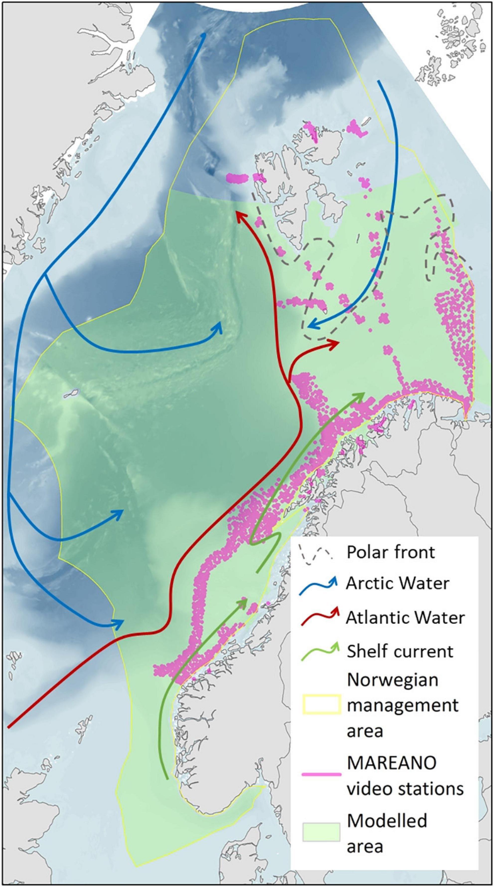
Figure 1. Map of the study area. The study area map includes approximate directions of dominant currents and the polar front which forms a putative biogeographic boundary, together with the modelled area (restricted by mapped environmental layer coverage), and the locations of MAREANO video transects that were used as the basis of this work.

The oceanography of the area is mostly dominated by northward flowing Atlantic Water (AW), Arctic Intermediate Water (AIW), and Norwegian Sea Deep Water (NSDW) on the west coast of Norway, while Arctic Water (ArW) flows southwards encroaching into the north of the Barents Sea region. The associated characteristic properties of these water masses can help us to interpret our results and define whether each sea pen taxa may be confined to any particular water mass.

The AW is characterised by salinities over 35 g/kg with variable warmer temperatures and a lower boundary at ∼400–800 m (Blindheim and Rey, 2004). Below this, the cooler water masses are recirculated from Greenland. AIW has salinities between 34.87 and 34.91 g/kg (a salinity minimum on the slope) with temperatures between –0.5 and 1°C and predominantly occurring between ∼400 and 1000 m (Blindheim, 1990; Blindheim and Rey, 2004; Jeansson et al., 2017). At the deepest extent of our observations, below ∼1000 m, NSDW is < –0.5°C, with salinities between 34.91 and 34.92 g/kg (Blindheim and Rey, 2004). In the shallower Barents Sea, there is also a biogeographic boundary represented at least partially by the polar front (Lacharité et al., 2016; Buhl-Mortensen et al., 2020) where the northward flowing cooling AW meets southward flowing Arctic water (ArW). Similar to the AIW, ArW has low temperatures (<0°C) and low salinities (<34.7 g/kg) due to the influence of ice meltwater, with its position partly related to the extent of ice cover each year (Barton et al., 2018).

All study taxa show potentially circum-global distributions particularly as pooled genera or families (Williams, 2011; GBIF download, 2020a,b,c,d,e,f). The study area, while only covering part of their ranges, has the potential to represent the northern extent of some of these taxa, giving a chance of encountering niche limits (sub-optimal environments) especially where the polar front may offer a distinct biogeographic boundary (Hargreaves et al., 2014).

Taxa Data

The MAREANO dataset used in this study comprises georeferenced observations from second-by-second video analysis of standardised benthic video transects, each ∼800 m length. These data were collected on 28 cruises between 2006 and 2019, using either the “CAMPOD” or “Chimaera” camera systems (described in Buhl-Mortensen et al., 2009, 2012; Buhl-Mortensen and Buhl-Mortensen, 2017) with HD video cameras at a 45° angle, and annotated in a custom-made software: VideoNavigator (described in Gomes Pereira et al., 2016). More details are available in Buhl-Mortensen et al. (2020) and Gonzalez-Mirelis et al. (2021).

While a fully quality controlled and quantitative dataset will become available soon (the MAREANO Video Database, ‘MarVid,’ Gonzalez-Mirelis et al., 2021), this study used semi-quantitative (i.e., counts are approximate) field data from 2051 video transects (the ‘MarBunn’ field dataset can be made available upon request to nmd@imr.no).

The MarBunn dataset may suffer from some additional errors due to the on-the-fly nature of its analysis, but these were resolved as far as possible. The data was cleaned of misspellings and common names to ensure consistent naming of all sea pen taxa. All sea pen records at species level were taken as the primary group of taxa. Genus level data was also consolidated with these datasets to ensure that the presence dataset size was > 15 presence points at a scale of one presence point per 400 m pixel. Genus level records may, at any rate, be due to lack of visibility or distance from the camera reducing video-based taxonomic ID confidence. A preliminary environmental analysis (histograms per taxa per environmental variable, see below) revealed that several of the assumed species-level taxa may be representative of more than one species due to bi-modalities and literature searches indicating alternative occurrences in the study region. These records were therefore elevated to the finest resolution higher taxonomic level that seemed likely based on historic physical sampling records in the region. This meant that two taxa were raised to genus level (Halipteris spp., Umbellula spp.), and two to family level (Pennatulidae spp., Virgulariidae spp.).

All georeferenced taxa observations were mapped in ArcGIS 10.6.1 and ‘rogue pings’ (produced by un-quality-controlled georeferencing) identified and removed from the analysis. The data resolution was coarsened to align with the full coverage environmental data (see below), resulting in one data point per 400 m (x400 m) pixel projected into Albers Equal Area Conic (parallel 1 = 55.8333, parallel 2 = 79.1666).

For this study, the sea pen dataset was reduced to presence/pseudo-absence records in the interest of consistency and quality control. Given the ∼3 m width of field of view of a video transect, while all records of target taxa could be considered to be presence points (P) at 400 m pixel resolution, their absence could not be guaranteed. Consequently, transect absences are considered to be pseudo-absences (psA), the concept of which is most important for the modelling process (see section “Modelling”).

A total of 6498 points of MAREANO video data were available for use at 400 m resolution, within 2051 video transects (see section “Modelling” for P:psA ratios per taxa).

Further presence data for ground-truthing purposes (an external independent test dataset) was obtained from:

– GBIF¹ (GBIF download, 2020a,b,c,d,e,f) – presence only data.

– a southern Norway survey report freely available online (OCEANA, 2018) – presence/pseudo-absence data.

– Selected unused MAREANO pseudo-absence data and the few unused presence points that did not have all environmental data layers overlapping them.

Note, this was not data gathered for the purpose of ground-truthing models, so their unbalanced distribution and varying dataset sizes are not ideal for this purpose. Consequently results should be interpreted with caution.

The data was cleaned to ensure that all points fall within the study area, are reduced to 1 point per 400 m pixel, and pseudo-absence points from OCEANA (2018) and MAREANO datasets were pooled and selected from using the same criteria as the main modelling selection (see section “Modelling”: must be between 5 and 300 km of a presence point then randomly selected to ensure a 2:1 ratio relative to the presence points). The final ground-truthing dataset comprised of (p:psA): 33:66 F. quadrangularis, 10:20 Halipteris spp., 109:218 K. stelliferum, 256:512 Pennatulidae spp., 4:8 Umbellula spp., 403:806 Virgulariidae spp. Maps of these ground-truthing presence and psA points are provided as insets to the predictive distribution maps.

Environmental Data

Mapped environmental variables were selected to maximise coverage of the study area, capture conditions likely to influence sea pen distribution, and be up- or downscale-able to 400m resolution (i.e., displaying one datapoint for every 0.16 km²).

The following “parent” variables were considered for evaluation (numbers in brackets represent the number of “sub-variables” within these, e.g., fine scale, broad scale, average, min, max, etc. There were 36 sub-variables considered. Brief summaries are given here, but more details are available in Supplementary Material.):

– bathymetry and derivatives: bathymetry, slope, topographic position index (TPI, 2), vector ruggedness measure (2), relative relief, bathy-based water mass.

– geological variables: landscape, valleyness, sediment (5).

– physical variables: carbon biomass of phytoplankton (2), current speed (2), chlorophyll a, dissolved oxygen (2), distance to shore, ice cover (2), silicon, salinity (4), temperature (4), temperature-based water mass, and Temperature/Salinity (TS) interaction.

All “parent” variables were re-projected into Albers Equal Area Conic (parallel 1 = 55.8333, parallel 2 = 79.1666, 400 m resolution) using the projectRaster function (Hijmans, 2020) with bilinear interpolation in R (R Core Team, 2020) before any “sub-variables” were derived.

The bathymetry was obtained from GEBCO Compilation Group (2019)² (accessed 27.01.2020) at 15 arc-second resolution (∼400 m in the study region). All bathymetry derivatives were generated in R (R Core Team, 2020) after reprojection, using the functions described in Supplementary Material. These sub-variables may act as proxies for otherwise uncaptured environmental data such as geomorphological features and their hydrodynamic influences (Wilson et al., 2007).

All geological variables originated from the Norwegian Geological Survey (NGU), with mapped polygon variables available for download from https://www.ngu.no/en/topic/datasets (accessed 24.03.2020). All polygons were converted to rasters with 400 m resolution. Some categories of the “Landscape” variable were combined after trials (see Supplementary Material). The “Valleyness” variable was derived from “Landscape” to provide an ordered categorical variable that describes how valley-like the landscape is [ranging from flat (0) to fjord (10), see Supplementary Material]. An ordered categorical variable is preferable in modelling, as predicted intermediate values can then be interpretable along the ordered scale. The “sediment” sub-variables were percentage sediment fractions and were converted from two combined categorical polygon maps (see Supplementary Material) into percentages using the conversion chart available here³. None of the geological variables cover the whole prediction area (∼60%). Consequently, a minimum of 2% was used for all sediment classes, such that it is always clear that 0% meant that there was no data present in a given area. The importance of sediment variables in the models is therefore likely to be underrepresented, but the histograms, PCAs, and model training data are based on locations where data is available so should reflect true patterns.

The remaining physical variables, mostly based on oceanographic models and remote sensing data, were obtained from bio-oracle⁴ (accessed 24.03.2020; Tyberghein et al., 2011). All but one of these variables were obtained for the bottom layer of the model (the “benthic” data layers), using the “mean depth” option where multiple depth readings were available. The exception was “ice cover” which necessarily is a surface variable and was used as a proxy for where the polar front/biogeographic boundary may occur. All bio-oracle data was downloaded at 5 arcminute resolution (∼8 km). This is undesirably coarse but the variables are potentially mechanistically important to the animals and needed to be represented – consequently all should be interpreted as being broadscale with local variations that are not captured in this analysis (interpolation to 400 m cannot add any detail).

Three further variables were derived and trialled to capture water mass structure. The trialled variables were derived from depth (“Bathymetry-based Water Mass,” based on Jeansson et al., 2017), Average Temperature (“Temperature-based water mass,” based on Blindheim, 1990), and Av. Temperature multiplied by Av. Salinity (“TS interaction”) respectively. The ‘TS interaction’ variable showed the most promise in this region (although it bares further development in the future) as the study area sees incursion of different types of arctic water in northern shallow water and in western deep water. Consequently depth- or temperature-only derived variables could not capture all possible water masses (although they may be adequate proxies in other regions of the globe).

All spatially aligned environmental variable values were extracted to the one-point-per-pixel P/psA locations using the ArcGIS spatial analyst extension.

Fishing Data

Fishing data from >15 m sized boats was obtained from the freely accessible Norwegian Electronic Reporting Service (ERS) dataset (Norwegian Fisheries Directorate, 2021) for a preliminary comparison to model maps. Norwegian fishing vessels are required to report the start and end of each fishing operation while at sea. Note that no foreign vessel data is included in this dataset. For the vessels that operate mobile, bottom-contacting gear (e.g., bottom trawls etc.), these two positions were interpolated into a straight line to approximate the path followed by the vessel, and therefore, the main impact footprint on the seabed. In order to account somewhat for interannual variability we used data for 4 years (namely 2017–2020). Fishing lines were converted to raster density layers (m/m2) per year within a cell size of 1000 m (this was deemed more appropriate than 400 m resolution given positional accuracy concerns). The average density for all 3 years was then calculated to approximate the location of common fishing grounds, and up-resolved to 400 m to compare with sea pen predictions.

Analysis and Modelling

All analyses were undertaken in R (R Core Team, 2020).

Data Exploration

The 36 environmental sub-variables at sample locations were plotted as individual histograms against presence data in order to provide a visual assessment of value ranges and data distributions. As spurious results are possible in modelled variables, the peak (most frequent) values within average/minimum/maximum variable histograms were given more credence than the extremes (e.g., the minimum of minimum/the maximum of the maximum).

A variance inflation factor (VIF) analysis was undertaken (using the usdm package; Naimi et al., 2014) to provide a more refined list of variables to work with in interpretations and modelling. The VIF is equivalent to 1/(1-R2) per variable (when that variable is regressed against all other variables, but not the response variable). This provides a way of identifying the variables which are most collinear with others. Typically, the variable with the highest VIF is removed stepwise to be as objective as possible (e.g., Yesson et al., 2017), but we chose to employ expert judgement, giving preference to the retention of variables which were likely to be more mechanistically relevant or intuitive than one of their strong correlates. This was supplemented by a correlation analysis to identify correlated sets of sub-variables to select from. The remaining variables had a VIF < 3.7, and a maximum correlation of | 0.6|.

The following 14 sub-variables (of the original 36 listed in Supplementary Material) were retained after the VIF selection process: bathymetry, carbon biomass of phytoplankton, maximum current speed, distance to shore, average ice cover, salinity range, % gravel, % mud, % sand, slope, temperature range, fine-scale TPI, valleyness, and TS interaction. These were used as the base “14 variable” dataset for the first set of models and all environmental analyses. (A subsequent reduction to eight variables was done in a second round of modelling to attempt to control for overfitting due to model complexity. See section “Modelling”).

Principle Component Analysis (PCA) biplots were made both prior to and after the VIF selection process, giving another perspective of variable importance and collinearity, and providing a means to examine any observable patterns displayed by presence locations as plotted in environmental space.

The co-occurrence of taxa in the dataset was examined as a means of understanding where environmental niches may be similar. Based on the presence or absence of the six taxa per video transect, the co-occur package (Griffith et al., 2016) utilised the probabilistic model of species co-occurrence (Veech, 2013) to compare the observed and expected frequencies of co-occurrence between each taxa pair. Results show whether there is a positive, negative, or random association between taxa.

Interpretations of all of these data explorations contribute toward the inferred likely habitat preference for each taxon; all of which were compared to international literature where possible. As comparisons to higher level taxon environmental profiles are problematic to interpret (they may be very vague), comparisons for each of these taxa are made with the most likely species-level taxon to be occurring within Norwegian waters, with an understanding that there may be records for other species in the dataset. Therefore, environmental profiles are compared with the literature profiles of Halipteris finmarchica for Halipteris spp., Pennatula phosphorea for Pennatulidae spp., Umbellula encrinus for Umbellula spp., and Virgularia mirabilis for Virgulariidae spp. [decisions informed by Directorate for Nature Management (2001) report, GBIF records (GBIF download, 2020a,b,c,d,e,f), the Norwegian Species Database⁵ and OCEANA (OCEANA, 2018; Álvarez et al., 2019) records].

Modelling

The psA classification of the absence records (as described in section “Taxa Data”) was intended to function more like background data while adjusting for the bias of the survey area (sensu Phillips and Dudík, 2008). However, as psA dominance relative to P locations can still bias model training (like absences), we first subset psA locations per taxon to optimise the training datasets, as advised by Lobo et al. (2010). Hutchinson (1957) described the concept of the fundamental and realised niches – the former shaped by environment alone, and the latter including the effects of impact and biotic interaction. Consequently Lobo et al. (2010) describe three types of absences: environmental (outside of both the fundamental and realised niches), contingent (outside the realised niche, but within the fundamental niche), and methodological (within both the fundamental and the realised niches, i.e., erroneous). The psA subsets were therefore designed to minimise the methodological absences and reduce the number of irrelevant environmental absences whilst maintaining a reasonable prevalence (i.e., proportion of P:psA). In practice this meant retaining all P locations with associated environmental data (no NA values), and subsetting psA per taxon so that they were located between 5 and 300 km from a P location. A further random selection from within that psA subset was done to maintain a prevalence of 0.33 (1P:2 psA) after Liu et al. (2019). Consequently the data subsets had the following P:psA ratios (based on 1 location per 400 m pixel): F. quadrangularis – 104:208, Halipteris spp. – 15:30, K. stelliferum – 194:388, Pennatulidae spp. – 18:36, Umbellula spp. – 87:174, and Virgulariidae spp. – 175:350.

The SDMs were built using the Biomod2 package (Thuiller et al., 2020) which allows you to run several different types of model at once and subsequently create an ensemble prediction (Thuiller et al., 2009). Ensemble models have the advantage of stabilising uncertain predictions and providing a consensus that is more balanced than using one model alone (Grenouillet et al., 2011). Although an ensemble may not outperform a well-tuned individual model when using default settings (Hao et al., 2020), ensemble models do have the benefit of offering multiple input models to derive more understanding of spatial uncertainties and can still perform equally well or better with additional tuning (Grenouillet et al., 2011). After initial trials, four types of machine learning model were run within Biomod2 for this study: Generalised Boosted Models (GBM, Ridgeway, 1999), Classification Tree Analyses (CTA, Breiman, 1984), Random Forests (RF, Breiman, 2001), and maximum entropy models (Maxent, Phillips et al., 2006). While more types of model are available within biomod2, models were chosen based on authors experience levels and with due diligence applied to understanding settings, relevance, and interpretations. (For more information on the pros and cons of each algorithm see e.g., Zhang and Li, 2017; Liu et al., 2019; Hao et al., 2020).

Preliminary tests recommended that, for this study, GBMs should be run with 3000 trees and an interaction depth of 3; RFs with a node size of 1; and Maxent with background data sampled from environmental rasters up to a maximum of 388 points. The presence only Maxent models operate differently from the other algorithms, using background data instead of psA data for optimal functioning (it is possible to run them with psA + P points as a background, but that set up is not supported in biomod2). Therefore the Maxent models in this study were allowed to randomly sample background points from the environmental rasters, but the maximum number of background points was set to be equivalent to a 1:2 P:PsA ratio for the largest presence dataset i.e., 388 (2* 194 K. stelliferum presence points) after the advice of Liu et al. (2019). While the smaller datasets may therefore have larger than 2:1 ratios, at worst this means there are more background points than are needed and predictions should not be disadvantaged or biased as a result (Liu et al., 2019). All other settings (including all CTA settings) were left at biomod2 defaults.

As no two algorithm runs give the same answer, five runs were made with each model type, giving 20 model builds and predictions for the six taxa (i.e., 120 models). Each run used five-fold cross-validation (CV), training models on 4/5ths of the presence datasets and tested on the held out 1/5th portion. A blockCV approach was used to spatially stratify the training and test data using the same method as Hao et al. (2020): briefly, the “blockCV” package (Valavi et al., 2018) was used, with the ‘spatialAutoRange’ function calculating the optimal size of blocks. The ‘selection = random’ argument was used in the ‘spatialBlock’ function to map and assign block and fold distribution in a suitable format for a ‘BIOMOD2’ ‘DataSplitTable’). This technique is used to combat issues of spatial autocorrelation and overfitting and to better approximate an independent test dataset (Valavi et al., 2018).

As it is generally advisable to use multiple evaluation metrics, the True Skill Statistic (TSS), Relative/Receiver Operating Characteristic (ROC), Cohen’s Kappa/Heidke skill score (KAPPA) and frequency bias score (BIAS) were calculated as evaluations of CV model accuracy. TSS represents how well the forecast separates “yes” from “no” events as values between –1 and 1, where 0 shows no skill. ROC is the hit rate vs. the false alarm rate with results between 0–1 and 0.5 represents no skill. KAPPA gives the fraction correctly classified excluding the proportion expected to be correct due to random chance and gives values from –1 to 1 with ≤0 being no skill. BIAS measures the frequency of forecast events compared to observed events to highlight under-forecasting (values < 1) or over-forecasting (values > 1) (Allouche et al., 2006; Wunderlich et al., 2019).

All 120 models were projected onto a stack of 14 environmental variable rasters to produce predictions for the whole study area. Each model also produced variable importance scores which were ranked and used to contribute to the assessments of preferred environmental conditions obtained from data exploration.

As using 14 environmental variables as predictors has the potential to cause overfitting due to the creation of over complex models, all models were then re-generated using the top 8 variables from the 14 variable constituent model runs, ensuring that the top two from each taxon were included. This generated another 120 models using the following 8 predictors as a basis: bathymetry, carbon biomass of phytoplankton, maximum current speed, distance to shore, percentage of gravel, percentage of mud, slope, and TS interaction.

Two ensemble models were then forecast for each taxon, one formed from the mean of all model runs within the 14 variable set, and the other from the mean of all models in the 8 variable set. While constituent runs had differing performance scores, no weightings were given to constituent models as the poor runs should not exert undue influence over the ensemble (Hao et al., 2020). Results from both ensemble predictions are evaluated for all taxa on the basis that consistencies and inconsistencies between them can further highlight prediction uncertainty/stability. Ensemble models were again assessed using TSS, ROC, KAPPA, and BIAS scores, and variable importance rankings produced.

Committee averaged (CA) predictions and Coefficient of Variation (CoV) maps were produced to accompany ensemble maps to provide more insight into spatial uncertainty. CA averages the binary (predicted presence or absence) output of all thresholded constituent models, here optimised by TSS scores. This provides a combined prediction and uncertainty score since values closer to 0 or 1 show agreement between constituent models on predicted absence and presence respectively, while values closer to 0.5 show disagreement. CoV maps show the s.d./mean for all pixels cross constituent models giving higher values where there is more variation in prediction scores.

Additionally a clamping map was produced per taxon showing where environmental values are outside of the trained range (based on the full 14 variable dataset) highlighting where uncertainty may stem from unsampled conditions (these can be found in Supplementary Material).

The 14 variable and 8 variable ensemble prediction rasters were intercompared using a Pearson Correlation Coefficient to assess the spatial similarity of model predictions both within taxa between the different variable sets, and across taxa to assess predicted co-occurrence.

Similarly, the Pearson Correlation Coefficient was also calculated for all ensemble model predictions relative to the fishing activity dataset. This gives an approximate score for the potential for impact.

Results

Environmental Profiles and Comparison With International Literature

An interpretation of the environmental profiles of each of these taxa, based on histograms of observations related to environmental data layers (Figure 2 and Supplementary Material) is shown in Table 1. Of the six taxa studied, Umbellula spp. appear to prefer the deepest water (∼800 m), and K. stelliferum the shallowest (∼200 m), although Pennatulidae spp. have the shallowest depth range (max 550 m). Umbellula spp. are found in the coolest temperatures (av. 1.3°C, min –1°C), but Virgulariidae spp., being present in ArW, are also very tolerant of cold water (a peak at 3.5°C, min –0.5°C). Pennatulidae spp. have the widest salinity tolerance (min peaks 33.7–34.5 g/kg, max 34.6–35.3 g/kg) and both Pennatulidae spp. and F. quadrangularis seem to favour areas with weaker currents (∼0.07 m/s, P. spp.: max 0.2 m/s, F. q.: 0.28 m/s) than the other taxa. Most taxa seem to favour flatter areas in valleys, canyons, or fjords, but Umbellula spp. are more likely to be found on the slope. Halipteris spp. have the greatest affinity for coarse gravelly sediments, and the least preference for mud, although Pennatulidae spp. also seem to prefer lower mud contents always being found with some proportion of sand. Umbellula spp. and Virgulariidae spp. have the most variable association with mud proportions suggesting a potential wider tolerance for varying sediment types than the other taxa (but sediment maps are coarse and do not preclude local variability).

FIGURE 2

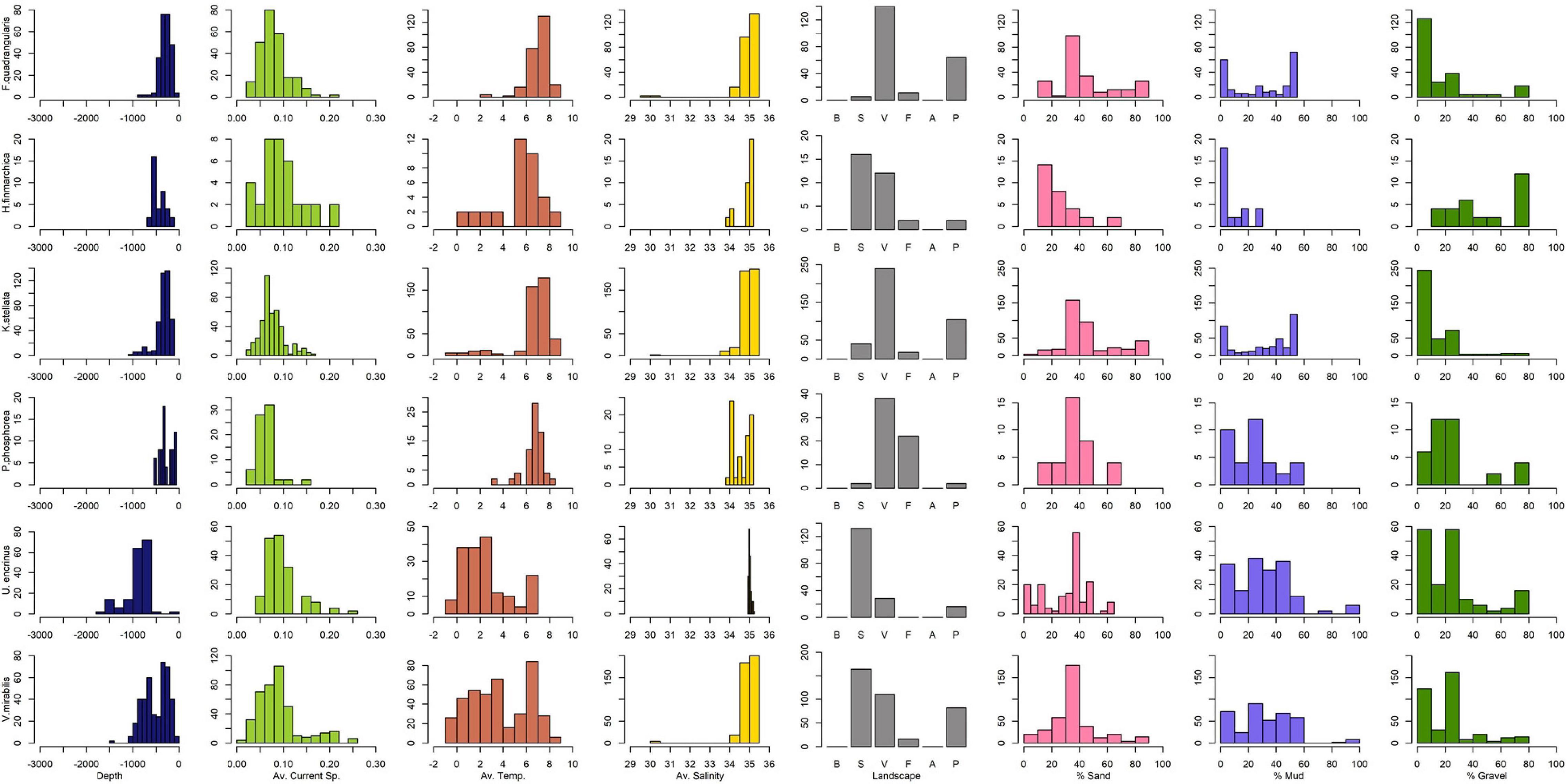
Figure 2. Selected histograms showing the distribution of presence locations relative to each environmental variable. Further histograms are available in Supplementary Material. The x-axis is scaled to show all possible values within the sampled area (values beyond this range may be present in the greater study area). Landscape categories represent: B, sandbank/strandflat; S, slope; V, valley/canyon; F, fjord; A, abyss; P, shelf plain. Sediment values are shown only for where sediment data is available – these three categories are scaled to the maximum y-axis of the three to better visually assess the proportion of one relative to another.

TABLE 1

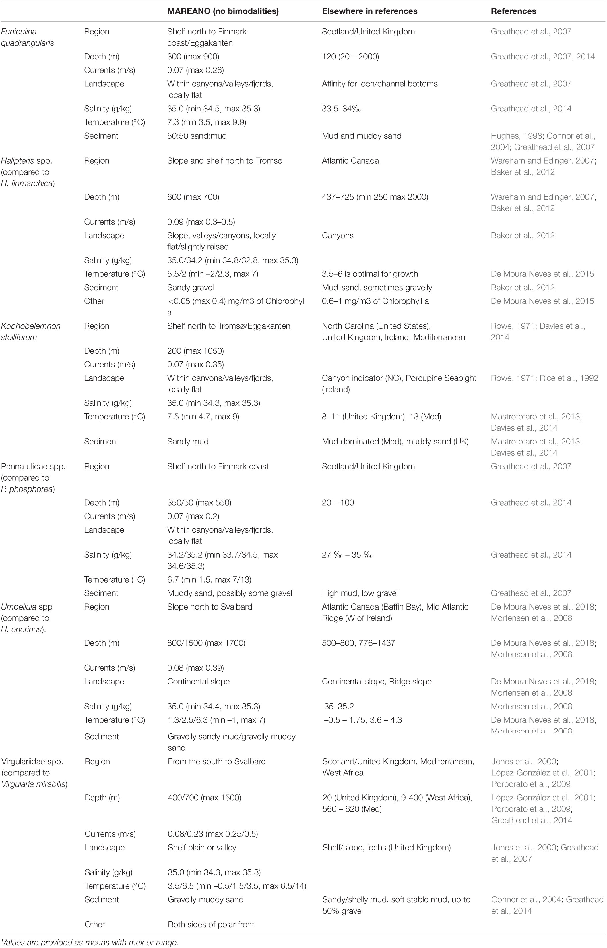
Table 1. Interpreted environmental preferences for each sea pen species (or group of species) for the MAREANO data (this study, based on peaks in histograms and observed distributions), and literature comparisons from elsewhere in the world.

Two taxa stood out as being the most inconsistent with the international literature: F. quadrangularis (depth and sediment disparities) and Virgulariidae (depth disparities when compared with V. mirabilis). In this study F. quadrangularis was found down to 900 m, optimally 300 m, while Greathead et al. (2007, 2014) stated an optimal depth of 120 m down to a maximum of 2000 m in Scotland. Virgulariidae had optimal peaks at 400/700 m, max 1700 m, in this study, while V. mirabilis is said to have an optimal depth of 20 m in Scotland (Greathead et al., 2014) and is found between 9 and 400 m in West Africa (López-González et al., 2001). F. quadrangularis also appeared to prefer 50:50 sand/mud with sand being the prerequisite in this study, while in Scotland they seem to prefer mud and sometimes muddy sand (Hughes, 1998; Connor et al., 2004; Greathead et al., 2007).

Taxa Co-occurrence

Comparisons of the observed and expected frequencies of co-occurrence between each pair of taxa (based on the probabilistic model of species co-occurrence (Veech, 2013) found that there were more negatively associated pairings (seven pairs) than random co-occurrences (six pairs) or positive associations (two pairs, Pennatulidae spp./Halipteris sp. and K. stelliferum/F. quadrangularis) (Figure 3). Support for these results can be seen in observation records and PCA results (see Supplementary Material). Across the 2051 video transects (VLs) analysed, 321 VLs recorded one or more sea pen taxa (an average of 1.3 taxa) and only 79 VLs recorded two or more co-occurring sea pen taxa (24% of VLs displayed an average of 2.24 taxa). Only one video transect (VL701) recorded 5 of the 6 taxa co-occurring. The maximum co-occurrence of any two taxa per video transect was always less than 50%. PCA results show partially overlapping environmental space between taxa, but none overlap completely. Co-occurrence records and PCA results agree that Pennatulidae spp. co-occurred the most with other taxa (66.7%) while Virgulariidae spp. co-occurred the least (30.0%).

FIGURE 3

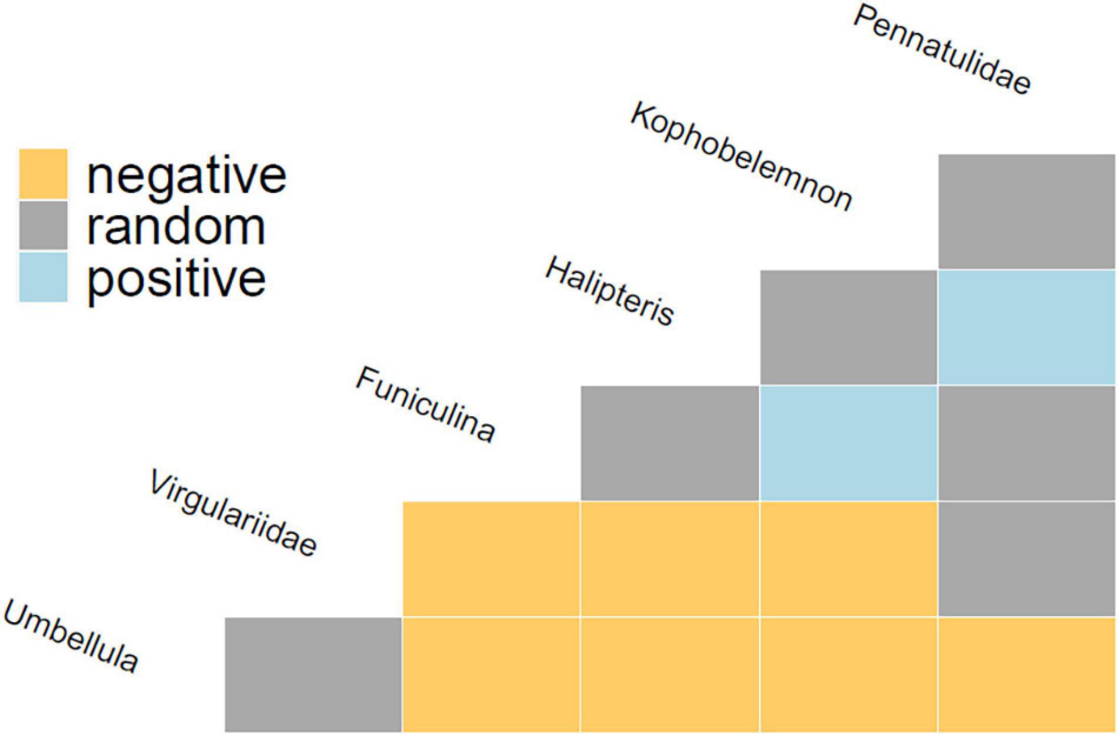
Figure 3. Taxon co-occurrence matrix output from the co-occur package in R. This shows comparisons of observed and expected frequencies of taxon co-occurrence based on Veech (2013) probabilistic model of species co-occurrence. Positive patterns suggest a high likelihood of co-occurrence, while negative have a low likelihood of co-occurrence, and random show no discernible pattern.

Predicted distribution maps output by the SDMs (Figure 4) also show there to be clear differences between the predicted distributions of most taxa, although there are also suggestions of some similarities. Pearson correlations of model predictions for F. quadrangularis and K. stelliferum were moderately strong (0.589 in 14 variable ensembles, 0.724 in 8 variable ensembles, Table 2) and appear to show similar predicted distributions in the south around the Norwegian Trough and on the mid-Norwegian shelf (∼60°N). However, those patterns diverge in the Barents Sea region, showing that the predicted niches may overlap but are not consistent between the two taxa. Co-occurrence records (Supplementary Material) confirm that these taxa were observed to co-occur the most of any two taxa in this study with K. stelliferum appearing at 46% of F. quadrangularis occurrences, and F. quadrangularis appearing at 30.1% of K stelliferum occurrences. All other Pearson correlation coefficients between taxa showed weak (| 0.2| –| 0.5|) or no correlation (<| 0.2|).

FIGURE 4

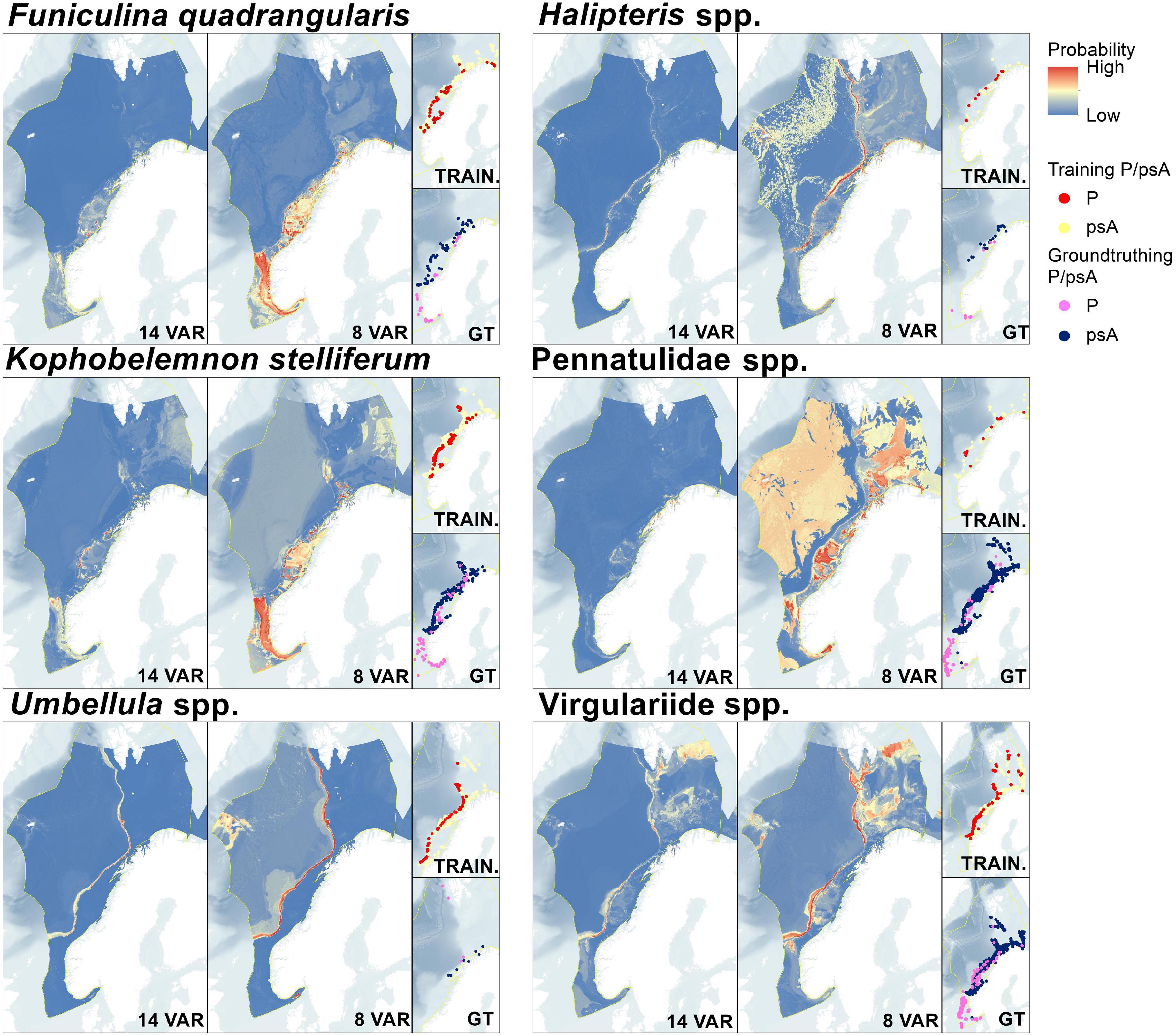
Figure 4. Fourteen and eight variable prediction maps from ensemble SDMs for each taxon, together with inset maps displaying training and ground-truthing Presence/pseudoAbsence locations.

TABLE 2

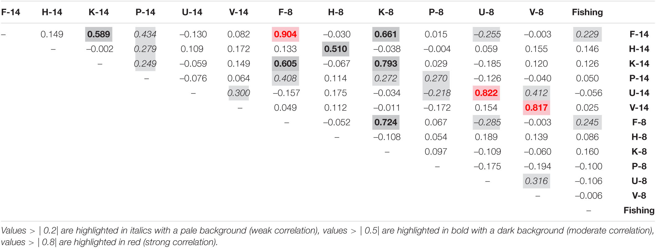
Table 2. Pearson correlation coefficients between all prediction rasters (14 variable and 8 variable predictions per taxa: F, Funiculina quadrangularis; H, Halipteris spp.; K, Kophobelemnon stelliferum; P, Pennatulidae spp.; U, Umbellula spp., V - Virgulariidae) and the fishing raster.

These findings suggest that it is unwise to treat sea pen taxa as a coherent group in analyses.

Model Predictions, Uncertainty and Data Quality

All models suffered from some level of overfitting which is apparent from evaluation scores. Species distribution modelling internal evaluation scores for both the 14 variable and the 8 variable ensembles are high (min 0.85, Table 3), but external evaluation scores are generally much poorer and ranged from high (0.91) to negative values (i.e., worse than a random guess, Table 3). Note however that the spatially unbalanced nature of the ground-truthing datasets and the small ground-truthing datasets for Halipteris spp. and Umbellula spp. especially may bias these external evaluation scores.

TABLE 3

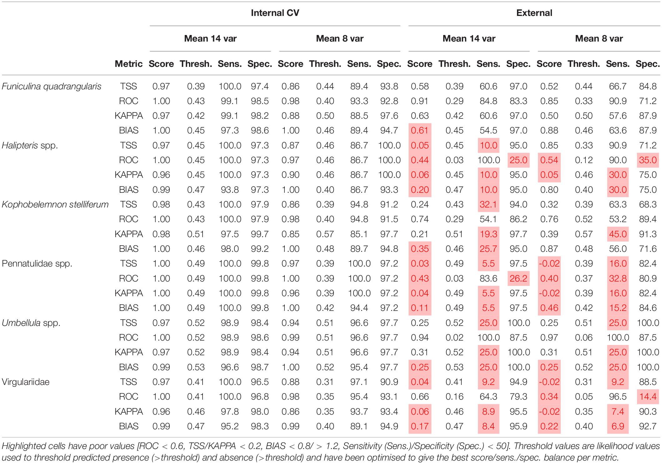
Table 3. Summarised model evaluation scores for the internal and external ensemble model predictions.

Generally the two species-level taxa provided the most reliable predictions (F. quadrangularis, K. stelliferum), while higher taxonomic level taxa, and taxa with small training datasets produced poorer predictions. All 14 variable ensembles appear to be underpredicting according to external evaluations (BIAS < 0.8), while only half of the 8 variable ensembles underpredict (Pennatulidea spp., Umbellula spp., Virgulriidae spp.). Bathymetry and TS interaction were the most important variables overall, with the 14 variable ensembles generally relying upon one variable above all others, while half of the 8 variable ensembles placed value (>0.1) on two or more variables (Table 4).

TABLE 4

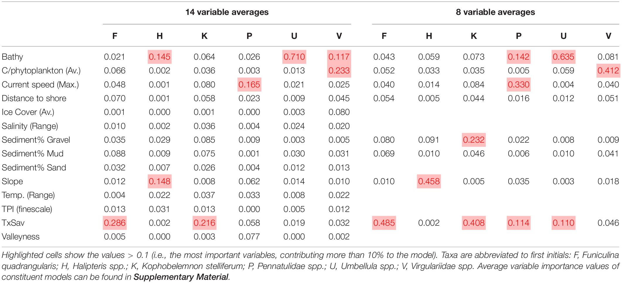
Table 4. Average permuted variable importance from ensemble models per taxon for both the 14 variable and 8 variable ensemble models.

The F. quadrangularis SDM performed the best of any of the target taxa with adequate sensitivity and specificity scores even in external evaluations (Table 3). The 14 and 8 variable predictions are spatially aligned south of Bjørnøya although the likelihood levels were different (Figure 4), and the 8 variable prediction appeared to give the most consistent likelihood values (Figure 5). TS interaction was the most important variable in both 14 and 8 variable ensembles (Table 4).

FIGURE 5

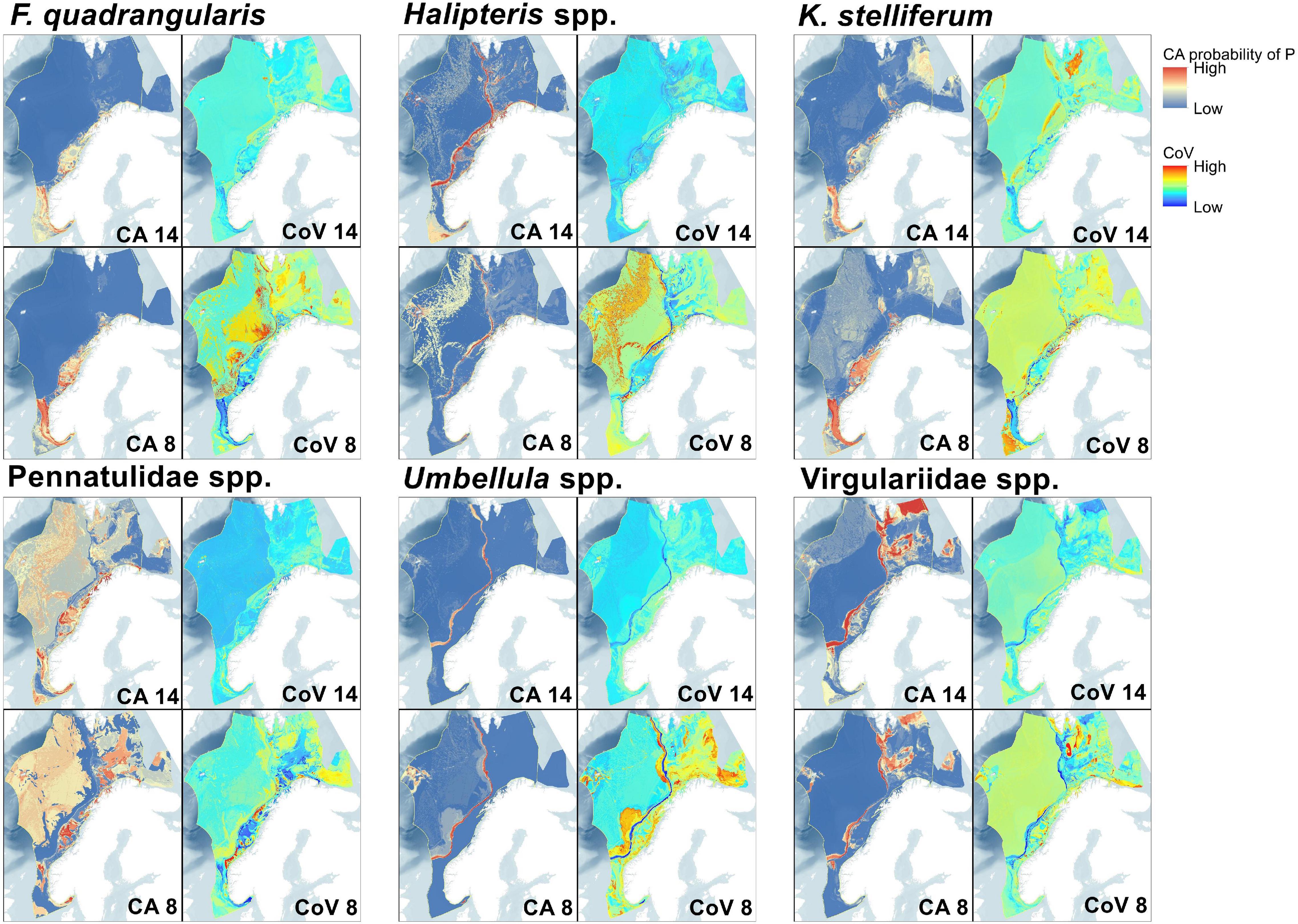
Figure 5. Maps representing spatial uncertainty in predictions for both the fourteen and eight variable predictions. Committee averaged (CA) predictions combine prediction and uncertainty by averaging the likelihood of presence after conversion to a binary presence/absence prediction (here using the TSS score thresholds shown in Table 2), consequently these predictions include some measure of uncertainty as scores closer to 0 or 1 have greater consensus, while 0.5 shows disagreement. Coefficient of variation (CoV) displays the S.D./mean of all probabilities across models and therefore higher values show locations with greater variation in predictions.

The K. stelliferum prediction gave an adequate ROC-based sensitivity and specificity balance in external evaluations (Table 3) but performed poorly with 14 variables when assessed with all other metrics (i.e., sensitivity < 50), and with 8 variables when assessed with KAPPA. There was greatest consistency in prediction of presence within the Norwegian Trough region (especially for the eight variable ensemble) and near the mid-Norway shelf edge (Figures 4, 5). TS Interaction was important to both ensembles, with proportion of gravel also being a strong predictor in the eight variable ensemble (Table 4).

Halipteris spp. and Pennatulidae spp. produced the worst predictions with strong inconsistencies between 14 variable and 8 variable predictions (Figure 4). Pennatulidae spp. in particular displayed little consistency between ensemble predictions (corr. 0.270, Table 2) and produced some spurious predictions in the deep sea west of the shelf. Both of these taxa had very small training datasets (Halipteris spp. 16 presence points, Pennatulidae spp. 32). It should be noted, however, that CA maps (Figure 5) show there are some locations where 14 and 8 variable predictions consistently predict presence: the shelf edge for Halipteris spp. and the northern Norway Trough and mid-Norwegian shelf for Pennatulidae spp. Slope and depth (14 variable only) were important to Halipteris spp. predictions, and Maximum Current Speed and depth (8 variable only) for the Pennatulidae spp. predictions (Table 4).

Virgulariidae spp., despite having the second largest training dataset did not perform well in external validations (except for when assessed with an ROC-based threshold in the 14 variable model). Yet there is relative spatial consistency between the 14 and 8 variable predictions (corr. 0.817 Table 2 and Figures 4, 5). Carbon biomass of phytoplankton (both ensembles) and depth (14 variable ensemble only) were of greatest important to Virgulariide spp. ensembles.

The Umbellula spp. model performed the best out of the higher-level taxonomic groupings, but its external validation dataset was smaller than can give a meaningful assessment (sensitivity scores of 25 and 100%, Table 3, represent the ability to predict 1 of 4 and 4 of 4 ground-truthing presence points respectively). Bathymetry and TS Interaction (8 variable ensemble only) were the most influential predictors for Umbellula spp.

Correlations between all taxa ensemble predictions and the fishing intensity data (Table 2 and map available in Supplementary Material) suggest that F. quadrangularis may have the greatest overlap with fishing areas of all taxa, but the correlation was still low at max | 0.245| (8 variable ensemble prediction).

Discussion

The study aimed to develop environmental profiles and predicted distribution maps for six sea pen taxa in Norway and consider three management-relevant issues on an international level. Namely: do any of these sea pen taxa have differing environmental profiles between regions that might impact how they are managed? Is it appropriate to consider these taxa as a group i.e., as “sea pens” rather than at a species level? And what are the consequences of needing to identify taxa at higher taxonomic levels (as is often necessary)? Note that the models created in this study were generally overfitted i.e. model results should be interpreted with caution, placing trust only where there is consensus between fourteen and eight variable models/where spatial uncertainty is lowest. However, once the limitations of this study are understood, it is still possible to tentatively draw some conclusions that may be useful to management.

Limitations of This Study

While environmental profiles and predicted distribution maps were generated, it is important to understand the limitations of this study to interpret the results appropriately. Broadly the limitations fall into the categories of: coarse and indirect underlying predictors with their own associated uncertainties; some small training datasets; small, spatially biased and inconsistently sampled ground-truthing datasets; and poor taxonomic resolution (the latter is discussed further in section “What Are the Management Impacts of Taxonomic Identification Issues?”).

Both environmental profiles and model predictions are mainly limited by the resolution and availability of the underlying environmental predictors. All of these predictors come from models or interpolations in order to obtain enough data coverage, while variables such as “distance from shore” and terrain derivatives are proxies for more specific variables that might otherwise be uncaptured (e.g., the influence of freshwater/pollution, or hydrographic parameters/food availability respectively, Wilson et al., 2007). These are problems faced by all modellers and improving the explicitness of uncertainties, together with the availability and resolution of predictors is greatly needed to improve predictive performance (Bowden et al., 2021).

Training/ground-truthing dataset size and spatial bias are also very common problems amongst modellers. This training dataset was based on extensive survey data using standardised methods and wide spatial coverage. However, it still omits many areas that were predicted into (i.e., is spatially biased) and two taxa had low prevalence resulting in small training datasets (Halipteris spp. and Pennatulidae spp., with 16 and 32 presence points respectively). The consequence of small and spatially biased datasets is an incomplete characterisation of the taxon’s environmental niche resulting in models that may be unstable and overfitted (Hernandez et al., 2006; Liu et al., 2019). These issues are insurmountable without additional data to better characterise the niche. Consequently, the models for Halipteris spp. and Pennatulidae spp. in particular should be interpreted with caution, although spatial uncertainty maps can help to isolate areas of consistent prediction which may be more trustworthy.

The ground-truthing datasets suffered from further issues. Diverse sources, sampling methods, and dates of sampling introduce errors of spatial, temporal, and taxonomic uncertainty that are hard to quantify. Together with the size and spatial bias issues mentioned above, these external evaluations were not ideal. All of the ground-truthing data used in this study suffers from spatial biases (particularly with absences distant from presences) and Umbellula spp. and Halipteris spp. had very small prevalence in their external validation sets (4 and 10 presence points respectively). Arguably these two taxa should not have been externally validated until more data became available, but it is useful to recognise whether there is consistency in the prediction of these presence/absence locations while accepting that the evaluations are partial at best. Ideally a ground-truthing dataset would be collected explicitly for that purpose, aim to span the environmental niche as much as the geography, would have similar prevalence and size to the training dataset, and would have no spatial/environmental biases (Araújo and Guisan, 2006; Bowden et al., 2021). These data should be used to test models built on similarly acquired training data, and then incorporated into them, with iterative testing and training used to continually improve models while observations continue to be made (Bowden et al., 2021). More efforts need to be made to undertake this process and impress upon management the need to fund such a process in order to best support their needs.

Given these limitations of the training and ground-truthing datasets, model evaluation scores should be interpreted with caution. The high internal evaluation scores are typical when using internal cross validation as the model is testing itself on data that suffers from the same biases as the training data (Hao et al., 2020). The external evaluation scores likely suffer from the opposite effect, giving overly critical or at least unstable assessments of the predictions. A true evaluation is therefore likely to be somewhere between the internal and external scores.

While these limitations may not be encouraging, these outcomes are both not unusual and may still be useful to management. Bowden et al. (2021) recently re-assessed 47 habitat suitability models for benthic epifaunal invertebrate taxa in New Zealand against external data and also found reduced evaluation scores, with no trend of improvement with modern modelling techniques. Model results, when interpreted honestly and with explicit measures of spatial uncertainty can still offer some insight especially in areas where multiple models agree (Dolan et al., 2021). These are still an improvement on having no information about species or habitat distribution. This sentiment is echoed by the UN Decade of Ocean Science (2021–2030) which officially recognises the benefits of models for filling in data gaps and highlights the global need to direct research resources toward improving ocean predictions as one of the seven targeted “decade outcomes” (UN/IOC, 2020).

Also worth noting are that predictions into the Barents sea region, beyond an assumed biogeographic boundary around the polar front (Lacharité et al., 2016; Buhl-Mortensen et al., 2020) may not have adequately captured variables that map this polar front and the stark change from Atlantic to Arctic water that occurs there. While more efforts could go into capturing this boundary, there is evidence that the front is weakening and that the Barents Sea is becoming less stratified, warmer, and more saline in response to climate change (Barton et al., 2018; Lind et al., 2018). Consequently, it is possible that predictions that span the polar front (see Figure 1 for an approximate position) may highlight areas where the northern range of some of these taxa may expand into given continued warming. More work is required to investigate this further, but if it is true then such projections may be useful to marine managers planning for a warmer future.

Similarities and Disparities Between Environmental Profiles Highlight the Vulnerability of Funiculina quadrangularis

Despite some environmental profiles being less coherent than others, generally this study’s environmental profiles are fairly consistent with international literature. Even Halipteris spp., which gave the least coherent environmental profile and was based on the smallest dataset, displayed an affinity for canyons and sometimes gravelly sediments that is supported by Baker et al. (2012), and a depth range similar to those found in Atlantic Canada (Wareham and Edinger, 2007; Baker et al., 2012). Studies of optimal growth rates in H. finmarchica also showed a similar temperature profile to our records (3.5–6°C, aligning with our dominant histogram peak at 5.5°C), but highlighted a preference for a higher Chlorophyll a concentration than is typically found in Norwegian waters (0.6–1 mg/m³, max in study area 0.6 mg/m³; De Moura Neves et al., 2015). If Chlorophyll a really is important to Halipteris spp., this could explain the relative rarity of this taxon in Norwegian waters. Perhaps new presence records as the MAREANO programme continues, will help to refine these predictions in the future.

However, there were some notable disparities as compared to the international literature. Virgularia mirabilis being found considerably shallower than our Virgulariidae records in both Scotland and West Africa (López-González et al., 2001; Greathead et al., 2014), and F. quadrangularis being found to favour shallower waters and softer sediments in Scotland as compared to this study (Hughes, 1998; Connor et al., 2004; Greathead et al., 2007, 2014).

There are likely to be different reasons for these disparities. Virgulariidae spp. in particular were grouped at the family level due to bimodal histograms and records of multiple taxa from this family recorded in Norway that are hard or impossible to tell apart from video records alone. Assuming that V. mirabilis may be the dominant taxon from this family in Norway (Buhl-Mortensen et al., 2020) may have in fact been incorrect. V. tuberculata, in particular, is known to both co-occur with V. mirabilis in Norway (Directorate for Nature Management, 2001), and to have a more extended depth range than V. mirabilis (López-González et al., 2001). Therefore, it is possible that a greater prevalence of V. tuberculata than originally assumed could be masking the V. mirabilis signal in the histograms. However, other taxa could also be part of this confusion: V. glacialis and Stylatula elongata are also recorded from the study region (Directorate for Nature Management, 2001). It is therefore unsurprising that profiles did not match with those from other regions which may have fewer taxa from this Family present.

Funiculina quadrangularis, with both a depth and a sediment disparity, is unlikely to have similar taxonomic issues. Lozano et al. (Submitted) found F. quadrangularis in similar 50:50 sediments in the Gulf of Cadiz, but the Marine Habitat Classification for Britain and Ireland, for example, explicitly associate F. quadrangularis (Fun) with circalittoral fine mud (CFiMu) (biotope code “SS.SMu.CFiMu.SpnMeg.Fun”; Connor et al., 2004). The depth disparity (deeper in Norway than in Scotland) is also contrary to expectations when equivalent cool water temperatures should be found shallower the further north you travel. There are known anomalies in the North Sea which could potentially explain this depth difference (Knijn et al., 1993; Perry et al., 2005) but with inconsistencies in both depth and sediment preferences there may be another cause.

One theory for both depth and sediment differences is that there could be different “realised niches” (sensu Hutchinson, 1957) in different regions. The Norwegian F. quadrangularis model, although showing the most overlap with the fishing intensity data of all taxa modelled here, had only a low spatial correlation with fishing areas (max 0.245). It is possible that Norwegian F. quadrangularis are therefore less impacted than in other nations. Downie et al. (2021) showed that models built on the west or east coast of Scotland for F. quadrangularis suggest different niches, and attribute this to extensive bottom trawling in the UK North Sea modifying the east coast realised niche. Lozano et al. (Submitted) and Lauria et al. (2017) have found bottom trawling to be an important correlate when predicting the distribution of F. quadrangularis in southern Spain and Sicily, respectively, suggesting that the distribution of this species may be particularly impacted internationally. It is thought that the tall and brittle nature of this non-retractable sea pen species, may make F. quadrangularis particularly vulnerable to anthropogenic impact, e.g., from bottom trawling (Hughes, 1998; Greathead et al., 2007). If this is the case, then the collective findings of this study and the recent work of Lozano et al. (Submitted), Lauria et al. (2017), and Downie et al. (2021) add much stronger weight to the claims of Greathead et al. (2007): that F. quadrangularis warrants particular management focus (amongst sea pen taxa), with anthropogenic impact clearly shaping their distributions in multiple countries.

Should Norwegian F. quadrangularis be less impacted, it may be that this model better represents the “fundamental niche” of this species (sensu Hutchinson, 1957) when compared with the Scottish data. Both fundamental and realised niche maps are useful to management. Realised niche maps are useful when searching for the current distribution of a species, while the fundamental niche map, when compared to a realised niche map, may highlight additional areas that could be recolonised and recover from impact in the future. Future work will explore the case of F. quadrangularis in Norway further, and if found to be closer to the fundamental niche, then the environmental profile could be used to develop such maps in other more impacted nations using model transfer techniques (Yates et al., 2018). However, this study’s model may just represent another “realised niche” with modern day absences where habitat is actually suitable due to on-going impact (perhaps closer to the patterns seen in the Gulf of Cadiz (Lozano et al., Submitted), than those seen in Scotland). Given the lack of bimodalities in environmental profiles, the abundance of records, high performance of both internal and external evaluations, and low spatial uncertainties, the predictions for F. quadrangularis in this study are the most trustworthy, so we can at least be reasonably confident that we are capturing one or the other.

Sea Pens: Should They Be Considered as a Group in Analysis for Management?

As the order Pennatulacea is cited as a Vulnerable Marine Ecosystem (VME) indicator taxon in many regions⁶ and “Sea Pens and Burrowing Megafauna” is listed as an OSPAR habitat (OSPAR, 2010), there is a temptation to profile and model higher level taxa as a group to save time and effort and plan management decisions. While there are many genera within Pennatulacea (Williams, 2011) records of common co-occurrence may support regional decisions to group taxa in analyses to support management.

However, this study suggests that while sea pen taxa may co-occur in some parts of the study area, no two taxa were found to co-occur in more than 50% of locations, and some were inversely associated (see Figure 3). The lack of co-occurrence of V. mirabilis and P. phosphorea, in particular, may be surprising, as these taxa are listed in various habitat classifications as a common co-occurrence, especially in the United Kingdom [e.g., Jones et al., 2000, several EUNIS habitat classifications (EUNIS, 2019)⁷, and SS.SMu.CFiMu.SpnMeg in the Marine Habitat Classification (MHC) for Britain and Ireland JNCC (2015)]. Our limited Virgulariidae and Pennatulidae spp. co-occurrence observations may be symptomatic of our taxonomic resolution issue, with unknown proportions of our family level observations ascribed to those V. mirabilis and P. phosphorea specifically, and potentially again supporting the concept that V. mirabilis in particular is not the dominant species of Virgulariidae in Norway. Differing impact patterns in Norway may also be a possible reason for differing co-occurrence patterns, with V. mirabilis being brittle but retractile, and P. phosphorea being both retractile and flexible – these taxa therefore may have different chances of survival when encountering disturbance.

Regardless, both the EUNIS and MHC systems agree with our observations that there is not one habitat/biotope that captures all sea pen taxa, and while co-occurrences do happen, no two taxa are found to only co-occur with each other. We therefore advise that data grouped for analysis by scientists and consultants to support management planning should be based on ecological niche concepts at the taxon-specific, biotope-specific, or management-target species archetype (sensu Dunstan et al., 2011) level, with any further grouping only applied at the management level.

However, the “sea pens and burrowing megafauna” grouping my also be problematic at the management level. As F. quadrangularis seems to be the most provably vulnerable to anthropogenic impact of the sea pen taxa so far (Greathead et al., 2007; Lauria et al., 2017; Downie et al., 2021; Lozano et al., Submitted), it may be appropriate to take differing conservation actions for F. quadrangularis habitats as compared with other sea pen habitats. The “burrowing megafauna” requirement is also often overlooked, and remains vague as to whether it necessitates: the co-occurrence of a commercially valuable burrowing crustacean [e.g., Nephrops norvegica, as mentioned in OSPAR (2010)] as indicative of a higher potential for fishery impact, the presence of multiple soft sediment species (e.g., burrowing anemones or polychaetes) indicative of a high diversity habitat, or whether the presence of burrowing megafauna may be used to highlight areas of sea pen suitable habitat which are currently not colonised. Therefore the type of “burrowing megafauna” present may impact what management actions may need to be taken.

The “sea pens and burrowing megafauna” classification should therefore be thought of as a vague higher-level guide for both analysis and management actions, but at all times, in practice, should be divided into more appropriate smaller groupings for re-combination as conservation actions require. Indeed, it may be advisable to review the classification in the future to provide better management guidance and help define where priorities may lie. It is likely that similar analysis and management-action care should be taken with assumptions about other listed conservation habitats (e.g., “deep sea sponge aggregations,” “coral gardens,” etc.).

What Are the Management Impacts of Taxonomic Identification Issues?

Sometimes it is necessary to group taxa within, e.g., a genus, family or morphotype due to identification issues that were unavoidable during analysis. This study focussed on six sea pen taxa, of which two were assumed to be safe to identify at species-level (F. quadrangularis and K. stelliferum), while four, based on histogram bimodalities and literature cross-checks, were raised to genus-level (Halipteris spp. and Umbellula spp.), or family level (Virgulariidae spp. and Pennatulidae spp.). These were issues symptomatic of video analysis, where issues such as unclear imagery, distant observations, and lack of extreme close-ups or dissections affect the certainty of an identification (Howell et al., 2019).

Model results showed a clear difference between species-level and higher-level taxa predictions, with the higher-level taxa ensembles performing the worst. The Virgulariidae spp. models are the main example of this. While small training datasets could also be blamed for poor evaluations for two of the higher-level taxa (Halipteris spp., Pennatulidae spp.), the Virgulariidae spp. models, with the second largest training dataset (186 presence points, only K. stelliferum had more) also produced predictions with poor performance (Table 3). If this taxon had a Family specific niche, then with that much data we would expect stable environmental profiles, better evaluation scores, and predictions that do not cross a known biogeographic boundary around the polar front (Lacharité et al., 2016; Buhl-Mortensen et al., 2020). It is possible that some grouped taxa may be more viable to use in distribution models than others. SDMs (also known as ecological niche models) are only suited for characterising a single environmental niche (Smith et al., 2018). Allopatric divergence is thought to be the most common reason for speciation (i.e., caused by geographical isolation and resulting in clear environmental niche differences), although there are growing numbers of records suggesting that sympatric speciation does occur (driven by a local competition for resources which could translate into similar environmental niches; Dieckmann and Doebeli, 1999). Grouped taxon modelling would therefore be most suited to Genera/Families etc which have speciated sympatrically (Smith et al., 2018), or taxa grouped by a shared niche (i.e., biotope modelling or species archetype modelling, sensu Dunstan et al., 2011).

It therefore seems likely that the taxon observations grouped within the Virgulariidae spp. family in this study (see section “Similarities and Disparities Between Environmental Profiles Highlight the Vulnerability of Funiculina quadrangularis”) have sufficiently different niches to disadvantage grouped distribution modelling. These findings align with those of Bowden et al. (2021) who also noticed that taxonomic resolution impacted model performance, with the species-level models performing the best.

It should be noted that while taxonomic issues were assumed to be the cause of bimodalities in histograms, it is possible there were other reasons for the bimodalities. Sundahl et al. (2020) found similar bimodalities in reef histograms which are unlikely to be due to misidentification, instead attributing these to e.g., an uneven distribution of records in environmental space or a low importance of the variable in question. For this study, this may be the case for Umbellula spp. especially (i.e., perhaps these records do only represent Umbellula encrinus records), but without further investigations we cannot be sure and have chosen to be cautious and treat this taxon as potentially representative of more than one species. Known shallower Umbellula encrinus (Lindal Jørgensen et al., 2016) occurrences in the northern Barents Sea of may be useful in future models with wider predictor coverage to help expand the niche characterisation and discern differences in for example, depth and temperature requirements (which appear correlated in this dataset as occurrences did not span the polar front-related biogeographic boundary).

A precautionary approach to taxonomy is advisable as other studies have suffered from such issues before. Ross and Howell (2013) modelled the distribution of Lophelia pertusa reefs in the United Kingdom, but later found out that some deeper observations were likely to be Solenosmilia variabilis reef, making it more correct to define the model as predicting “Scleractinian reef” presence (Howell et al., 2014). This adjustment improved the performance of the models against ground-truthing data, and models were found to be adequate to characterise a common niche for the two reef types with depth bimodalities alone (as a proxy for water mass structure) helping to define where each species might be dominant (Howell et al., Submitted).

It is clear therefore that some taxonomic groupings or errors can impact management decisions, whether that be by providing erroneous or vague distribution maps, or by failing to identify rare/endemic species that should be of conservation interest. Fukami et al. (2004) found that assumed lower levels of endemism in the corals of the Atlantic as compared to the Pacific were false and had been masked by morphological convergence impacting taxonomic identification. As video and image observations are particularly prone to identification issues, it is wise for management decision-makers to assume that while more rare species could be identified than from physical sampling, there are some that would be identified in physical sampling that cannot be identified in imagery. To resolve this, much greater emphasis should be placed on ensuring best practices in taxonomic identification with better links between imagery, morphology and genetics to ensure consistency across sampling methods (Glover et al., 2016). In the meantime more efforts should be made to highlight where taxonomic uncertainties are present and unavoidable.

Conclusion

This study provides environmental profiles and distribution predictions for six sea pen taxa in Norway based on imagery analysis, data explorations and predictive modelling. Beyond this it finds that:

(a) External validation is important to understand the limitations of model predictions which may have deceptively high internal evaluation scores. But even poor models have some use when spatial uncertainty metrics can highlight areas of stable predictions.

(b) Disparities between the environmental profiles found in Norway and other parts of the world demonstrate that F. quadrangularis has different realised niches confirming that this taxon is likely to be particularly vulnerable to impact.

(c) Inconsistent co-occurrence of taxa suggests that sea pens should not be grouped in analyses to support management. Instead a taxon-specific/community-based analysis is advisable with any further consolidations being based on commonalities in management measures.

(d) Grouped taxa caused by identification issues may impact management decision-making as this can produce poorer environmental profiles and distribution maps. Predictive distribution models are based on environmental niches and require that the target taxon occupy a single environmental niche which is unlikely when taxa are grouped phylogenetically. Community/biotope groupings could provide one solution, while greater value should be placed on resolving taxonomy and quantifying the uncertainties that taxonomic issues present.

Data Availability Statement

The raw data supporting the conclusions of this article will be made available by the authors, without undue reservation.

Author Contributions

RR conceived the idea for the study, undertook the analysis, and wrote the manuscript. GG-M, PL, and PB-M variously consulted on the analysis and contributed to the writing. All authors contributed to the article and approved the submitted version.

Funding

This work was funded by the MAREANO programme through the Institute of Marine Research, Norway.

Conflict of Interest

The authors declare that the research was conducted in the absence of any commercial or financial relationships that could be construed as a potential conflict of interest.

Publisher’s Note

All claims expressed in this article are solely those of the authors and do not necessarily represent those of their affiliated organizations, or those of the publisher, the editors and the reviewers. Any product that may be evaluated in this article, or claim that may be made by its manufacturer, is not guaranteed or endorsed by the publisher.

Acknowledgments

Thanks to all participants in the MAREANO programme (the steering group, programme group, partners, leaders, and participants of all MAREANO cruises) and especially to the video analysis gurus: Gjertrud Jensen, Yngve Klungseth Johansen, and Anne Kari Sveistrup. Discussions with Anna Downie (CEFAS) have been very helpful to compare with ongoing work in the United Kingdom. The authors would also like to thank Dr. Laura Airoldi for her rewriting advice which resulted in a substantial improvement to the manuscript.

Supplementary Material

The Supplementary Material for this article can be found online at: https://www.frontiersin.org/articles/10.3389/fmars.2021.652540/full#supplementary-material

Footnotes

1. ^ https://www.gbif.org/
2. ^ https://gebco.net/
3. ^ https://www.ngu.no/Mareano/Kornstorrelse.html
4. ^ https://bio-oracle.org/
5. ^ https://artskart.artsdatabanken.no/
6. ^ http://www.fao.org/in-action/vulnerable-marine-ecosystems/vme-indicators/es/
7. ^ https://eunis.eea.europa.eu/index.jsp

References

Allouche, O., Tsoar, A., and Kadmon, R. (2006). Assessing the accuracy of species distribution models: prevalence, kappa and the true skill statistic (TSS). J. Appl. Ecol. 43, 1223–1232. doi: 10.1111/j.1365-2664.2006.01214.x

CrossRef Full Text | Google Scholar

Álvarez, H., Perry, A. L., Blanco, J., Conlon, S., Petersen, H. C., and Aguilar, R. (2019). Protecting the North Sea: Norway. Madrid: Oceana, 96.

Google Scholar

Araújo, M. B., and Guisan, A. (2006). Five (or so) challenges for species distribution modelling. J. Biogeogr. 33, 1677–1688. doi: 10.1111/j.1365-2699.2006.01584.x

CrossRef Full Text | Google Scholar

Baillon, S., Hamel, J. F., and Mercier, A. (2014). Diversity, distribution and nature of faunal associations with deep-sea pennatulacean corals in the northwest Atlantic. PLoS One 9:e111519. doi: 10.1371/journal.pone.0111519

PubMed Abstract | CrossRef Full Text | Google Scholar

Baillon, S., Hamel, J. F., Wareham, V. E., and Mercier, A. (2012). Deep cold-water corals as nurseries for fish larvae. Front. Ecol. Environ. 10, 351–356. doi: 10.1890/120022

CrossRef Full Text | Google Scholar

Baker, K. D., Wareham, V. E., Snelgrove, P. V. R., Haedrich, R. L., Fifield, D. A., Edinger, E. N., et al. (2012). Distributional patterns of deep.sea coral assemblages in three submarine canyons off Newfoundland, Canada. Mar. Ecol. Progr. Ser. 445, 235–249.

Google Scholar

Barton, B. I., Lenn, Y.-D., and Lique, C. (2018). Observed atlantification of the Barents Sea causes the polar front to limit the expansion of winter Sea Ice. J. Phys. Oceanogr. 48, 1849–1866.

Google Scholar

Blindheim, J. (1990). Arctic intermediate water in the Norwegian Sea. Deep-Sea Research 37, 1475–1489. doi: 10.1016/0198-0149(90)90138-l

CrossRef Full Text | Google Scholar

Blindheim, J., and Rey, F. (2004). Water-mass formation and distribution in the Nordic Seas during the 1990s. ICES J. Mar. Sci. 61, 846–863.

Google Scholar

Bowden, D. A., Anderson, O. F., Rowden, A. A., Stephenson, F., and Clark, M. R. (2021). Assessing habitat suitability models for the deep sea: is our ability to predict the distributions of seafloor fauna improving? Front. Mar. Sci. 8:632389. doi: 10.3389/fmars.2021.632389

CrossRef Full Text | Google Scholar

Breiman, L. (1984). Classification and Regression Trees. Belmont, CA: Wadsworth International Group.

Google Scholar

Breiman, L. (2001). Random forests. Mach. Learn. 45, 5–32.

Google Scholar

Bridge, T. C. L., Huang, Z., Przeslawski, R., Tran, M., Siwabessy, J., Picard, K., et al. (2020). Transferable, predictive models of benthic communities informs marine spatial planning in a remote and data-poor region. Conserv. Sci. Pract. 2:e251. doi: 10.1111/csp2.251

CrossRef Full Text | Google Scholar

Brodeur, R. D. (2001). Habitat-specific distribution of Pacific ocean perch (Sebastes alutus) in Pribilof Canyon, Bering Sea. Cont. Shelf Res. 21, 207–224. doi: 10.1016/S0278-4343(00)00083-2

CrossRef Full Text | Google Scholar

Buhl-Mortensen, L., and Buhl-Mortensen, P. (2017). Marine litter in the Nordic Seas: distribution composition and abundance. Mar. Pollut. Bull. 125, 260–270. doi: 10.1016/j.marpolbul.2017.08.048

PubMed Abstract | CrossRef Full Text | Google Scholar

Buhl-Mortensen, L., Buhl-Mortensen, P., Dolan, M. J. F., and Holte, B. (2015). The MAREANO programme – A full coverage mapping of the Norwegian off-shore benthic environment and fauna. Mar. Biol. Res. 11, 4–17.

Google Scholar

Buhl-Mortensen, L., Olsen, E., Røttingen, I., Buhl-Mortensen, P., Hoel, A. H., Lid, S. R., et al. (2012). Application of the MESMA Framework. Case Study: The Barents Sea. MESMA report, 138.

Google Scholar

Buhl-Mortensen, P., Buhl-Mortensen, L., Dolan, M., Dannheim, J., and Kröger, K. (2009). Megafaunal diversity associated with marine landscapes of northern Norway: a preliminary assessment. Norw. J. Geol. 89, 163–171.

Google Scholar

Buhl-Mortensen, P., Dolan, M. F. J., Ross, R. E., Gonzalez-Mirelis, G., Buhl-Mortensen, L., Bjarnadóttir, L. R., et al. (2020). Classification and mapping of benthic biotopes in arctic and sub-arctic norwegian waters. Front. Mar. Sci. 7:271. doi: 10.3389/fmars.2020.00271

CrossRef Full Text | Google Scholar

CBD (2009). Azores Scientific Criteria and Guidance for Identifying Ecologically or Biologically Significant Marine Areas and Designing Representative Networks of Marine Protected Areas in Open Ocean Waters and Deep sea Habitats. Secretariat of the Convention on Biological Diversity, Montreal. 12. Available online at: https://www.cbd.int/marine/doc/azores-brochure-en.pdf (accessed October 21, 2020).

Google Scholar

Clark, M. R., and Tittensor, D. P. (2010). An index to assess the risk to stony corals from bottom trawling on seamounts. Mar. Ecol. 31, 200–211. doi: 10.1111/j.1439-0485.2010.00392.x

CrossRef Full Text | Google Scholar

Colpron, E., Edinger, E. N., and Neis, B. (2010). Mapping the Distribution of Deep-Sea Corals in the Northern Gulf of St. Lawrence using Both Scientific and Local Ecological Knowledge. Canadian Science Advisory Secretariat (DFO). Available online at: https://waves-vagues.dfo-mpo.gc.ca/Library/340948.pdf (accessed July 27, 2021).

Google Scholar

Connor, D. W., Allen, J. H., Golding, N., Howell, K. L., Lieberknecht, L. M., Northen, K. O., et al. (2004). The Marine Habitat Classification for Britain and Ireland Version 04.05 ISBN 1 861 07561 8. In: JNCC (2015) The Marine Habitat Classification for Britain and Ireland Version 15.03. Available online at: https://mhc.jncc.gov.uk/resources#version0405 (accessed 23/03/2020).

Google Scholar

Crowder, L., and Norse, E. (2008). Essential ecological insights for marine ecosystem-based management and marine spatial planning. Mar. Policy 32, 772–778. doi: 10.1016/j.marpol.2008.03.012

CrossRef Full Text | Google Scholar

Davies, J. S., Howell, K. L., Stewart, H. A., Guinan, J., and Golding, N. (2014). Defining biological assemblages (biotopes) of conservation interest in the submarine canyons of the South West approaches (offshore United Kingdom) for use in marine habitat mapping. Deep Sea Res. II 104, 208–229.

Google Scholar

De Clippele, L. H., Buhl-Mortensen, P., and Buhl-Mortensen, L. (2015). Fauna associated with cold water gorgonians and sea pens. Cont. Shelf Res. 105, 67–78. doi: 10.1016/j.csr.2015.06.007

CrossRef Full Text | Google Scholar

De Moura Neves, B., Edinger, E., Hayes, V. W., Devine, B., Wheeland, L., and Layne, G. (2018). Size metrics, longevity, and growth rates in Umbellula encrinus (Cnidaria: Pennatulacea) from the eastern Canadian Arctic. Arctic Sci. 4, 722–749. doi: 10.1139/as-2018-0009

PubMed Abstract | CrossRef Full Text | Google Scholar

De Moura Neves, B., Edinger, E., Layne, G. D., and Wareham, V. E. (2015). Decadal longevity and slow growth rates in the deep-water sea pen Halipteris finmarchica (Sars, 1851) (Octocorallia: Pennatulacea): implications for vulnerability and recovery from anthropogenic disturbance. Hydrobiologia 759, 147–170. doi: 10.1007/s10750-015-2229-x

CrossRef Full Text | Google Scholar

Dieckmann, U., and Doebeli, M. (1999). On the origin of species by sympatric speciation. Nature 400, 354–357. doi: 10.1038/22521

PubMed Abstract | CrossRef Full Text | Google Scholar

Directorate for Nature Management (2001). Distribution of Marine, Benthic Macroorganisms in Norway: A Tabulated Catalogue. Research Report 2001-3 (Revised Edition of DN 1997-1), Trondheim, Norway. Available online at: https://www.miljodirektoratet.no/publikasjoner/publikasjoner-fra-dirnat/dn-utredninger/distribution-of-marine-benthic-macroorganisms-in-norway/ (accessed March 26, 2020).

Google Scholar

Dolan, M. F. J., Ross, R. E., Albretsen, J., Skarðhamar, J., Gonzalez-Mirelis, G., Bellec, V., et al. (2021). Using spatial validity and uncertainty metrics to determine the relative suitability of alternative suites of oceanographic data for seabed biotope prediction. A case study from the Barents Sea, Norway. Geosciences 11:48. doi: 10.3390/geosciences11020048

CrossRef Full Text | Google Scholar

Downie, A.-L., Noble-James, T., Chaverra, A., and Howell, K. L. (2021). Predicting sea pen (Pennatulacea) distribution on the UK continental shelf: evidence of range modification by benthic trawling. Mar. Ecol. Progr. Ser. 670, 75–91. doi: 10.3354/meps13744

CrossRef Full Text | Google Scholar

Dunstan, P. K., Foster, S. D., and Darnell, R. (2011). Model based grouping of species across environmental gradients. Ecol. Model. 222, 955–963.

Google Scholar

Food and Agriculture Organization [FAO] (2009). International Guidelines for the Management of Deep-Sea Fisheries in the High Seas. Rome: Food and Agriculture Organization.

Google Scholar

Fukami, H., Budd, A. F., Paulay, G., Sole-Cava, A., Chen, C. A., Iwao, K., et al. (2004). Conventional taxonomy obscures deep divergence between Pacific and Atlantic corals. Nature 427, 832–835. doi: 10.1038/nature02339

PubMed Abstract | CrossRef Full Text | Google Scholar

GBIF download (2020a). GBIF Occurrence Download: Funiculina quadrangularis (Pallas, 1766). Available online at: https://doi.org/10.15468/dl.vtk3qg (accessed November 23, 2020).

Google Scholar

GBIF download (2020b). GBIF Occurrence Download: Halipteris Kölliker, 1880. Avaialble online at: https://doi.org/10.15468/dl.w4znbr (accessed November 23, 2020).

Google Scholar

GBIF download (2020c). GBIF Occurrence Download: Kophobelemnon stelliferum (Müller, 1776). Available online at: https://doi.org/10.15468/dl.9uu3nw (accessed November 23, 2020).

Google Scholar

GBIF download (2020d). GBIF Occurrence Download: Pennatulidae. Avaialble online at: https://doi.org/10.15468/dl.vkf3f6 (accessed November 23, 2020).

Google Scholar

GBIF download (2020e). GBIF Occurrence Download: Umbellula Cuvier, 1797. Available online at: https://doi.org/10.15468/dl.dthzep (accessed November 23, 2020).

Google Scholar

GBIF download (2020f). GBIF Occurrence Download: Virgulariidae. Available online at: https://doi.org/10.15468/dl.2vumnu (accessed November 23, 2020).

Google Scholar

GEBCO Compilation Group (2019). GEBCO 2019 Grid. doi: 10.5285/836f016a-33be-6ddc-e053-6c86abc0788e

PubMed Abstract | CrossRef Full Text | Google Scholar

Glover, A. G., Dahlgren, T. G., Wiklund, H., Mohrbeck, I., and Smith, C. R. (2016). An End-to-End DNA taxonomy methodology for benthic biodiversity survey in the clarion-clipperton zone, Central Pacific Abyss. J. Mari. Sci. Eng. 4:2. doi: 10.3390/jmse4010002

CrossRef Full Text | Google Scholar

Gomes Pereira, J. N., Auger, V., Beisiegel, K., Benjamin, R., Bergmann, M., Bowden, D., et al. (2016). Current and future trends in marine image annotation software. Prog. Oceanogr. 149, 106–120. doi: 10.1016/j.pocean.2016.07.005

CrossRef Full Text | Google Scholar

Gonzalez-Mirelis, G., Ross, R. E., Abretsen, J., and Buhl-Mortensen, P. (2021). Modeling the distribution of habitat-forming, deep-sea sponges in the Barents sea: the value of data. Front. Mar. Sci. 7:496688. doi: 10.3389/fmars.2020.496688

CrossRef Full Text | Google Scholar

Greathead, C. F., Donnana, D. W., Mair, J. M., and Saunders, G. R. (2007). The sea pens Virgularia mirabilis, Pennatula phosphorea and Funiculina quadrangularis: distribution and conservation issues in Scottish waters. J. Mar. Biol. Assoc. U. K. 87, 1095–1103. doi: 10.1017/s0025315407056238

CrossRef Full Text | Google Scholar

Greathead, C., González-Irusta, J. M., Clarke, J., Boulcott, P., Blackadder, L., Weetman, A., et al. (2014). Environmental requirements for three sea pen species: relevance to distribution and conservation. ICES J. Mar. Sci. 72, 576–586. doi: 10.1093/icesjms/fsu129

CrossRef Full Text | Google Scholar

Grenouillet, G., Buisson, L., Casajus, N., and Lek, S. (2011). Ensemble modelling of species distribution: the effects of geographical and environmental ranges. Ecography 34, 9–17. doi: 10.1111/j.1600-0587.2010.06152.x

CrossRef Full Text | Google Scholar

Griffith, D. M., Veech, J. A., and Marsh, C. J. (2016). cooccur: probabilistic species co-occurrence analysis in R. J. Stat. Softw. 69, 1–17. doi: 10.18637/jss.v069.c02

CrossRef Full Text | Google Scholar

Hao, T., Elith, J., Lahoz-Monfort, J. J., and Guillera-Arroita, G. (2020). Testing whether ensemble modelling is advantageous for maximising predictive performance of species distribution models. Ecography 43, 549–558. doi: 10.1111/ecog.04890

CrossRef Full Text | Google Scholar

Hargreaves, A. L., Samis, K. E., and Eckert, C. G. (2014). Are species’ range limits simply niche limits writ large? A review of transplant experiments beyond the range. Am. Nat. 183, 157–173. doi: 10.1086/674525

PubMed Abstract | CrossRef Full Text | Google Scholar

Hernandez, P. A., Graham, C. H., Master, L. L., and Albert, D. L. (2006). The effect of sample size and species characteristics on performance of different species distribution modeling methods. Ecography 29, 773–785. doi: 10.1111/j.0906-7590.2006.04700.x

CrossRef Full Text | Google Scholar

Hijmans, R. J. (2020). raster: Geographic Data Analysis and Modeling. R Package Version 3.4-5. Available online at: https://CRAN.R-project.org/package=raster (accessed November 10, 2021).

Google Scholar

Howell, K. L., Bullimore, R. D., and Foster, R. D. (2014). Quality assurance in the identification of deep-sea taxa from video and image analysis: response to Henry and Roberts. ICES J. Mar. Sci. 71, 899–906. doi: 10.1093/icesjms/fsu052

CrossRef Full Text | Google Scholar

Howell, K. L., Davies, J. S., Allcock, A. L., Braga-Henriques, A., Buhl-Mortensen, P., Carreiro-Silva, M., et al. (2019). A framework for the development of a global standardised marine taxon reference image database (SMarTaR-ID) to support image-based analyses. PLoS One 14:e0218904. doi: 10.1371/journal.pone.0218904

PubMed Abstract | CrossRef Full Text | Google Scholar

Hughes, D. J. (1998). Sea Pens and Burrowing Megafauna: An Overview of Dynamics and Sensitivity Characteristics for Conservation Management of Marine SACs, Vol. III. Oban: Scottish Association of Marine Science, 105.

Google Scholar

Hutchinson, G. E. (1957). Concluding remarks. Cold Spring Harb. Symp. Quant. Biol. 22, 415–427.

Google Scholar

ICES (2020). ICES/NAFO Joint Working Group on Deep-water Ecology (WGDEC). ICES Scientific Reports. 2:62. 171. Available online at: http://doi.org/10.17895/ices.pub.6095 (accessed July 07, 2020).

Google Scholar

IUCN (2012). IUCN Red List Categories and Criteria: Version 3.1, Second Edn. Gland: IUCN, iv+32.

Google Scholar

Jeansson, E., Olsen, A., and Jutterström, S. (2017). Arctic intermediate water in the Nordic Seas, 1991–2009. Deep Sea Res. Part I Oceanogr. Res. Papers 128, 82–97.

Google Scholar

JNCC (2015). The Marine Habitat Classification for Britain and Ireland Version 15.03. Available online at: https://mhc.jncc.gov.uk/

Google Scholar

Jones, L. A., Hiscock, K., and Connor, D. W. (2000). Marine Habitat Reviews, a Summary of Ecological Requirements and Sensitivity Characteristics for the Conservation and Management of Marine SAC’s. UK Marine SAC’s Project report 17pp. Peterborough: Joint Nature Conservation Committee. Available online at: http://spcsrp.org/sites/default/files/csrp/ressouces_documentaires/marine%20habitat%20reviews.pdf (accessed July 23, 2020).

Google Scholar

Knijn, R. J., Boon, T. W., Heesen, H. J. L., and Hislop, J. F. G. (1993). Atlas of North Sea Fishes. International Council for the Exploration of the Sea (ICES) Cooperative Research Report 194, ICES, Copenhagen. Available Online at: http://www.vliz.be/imisdocs/publications/ocrd/120153.pdf (Accessed November 03, 2020)

Google Scholar

Lacharité, M., Lindal Jørgensen, L., Metaxas, A., Lien, V. S., and Rune Skjoldal, H. (2016). Delimiting oceanographic provinces to determine drivers of mesoscale patterns in benthic megafauna: a case study in the Barents Sea. Progr. Oceanogr. 146, 187–198. doi: 10.1016/j.pocean.2016.06.008

CrossRef Full Text | Google Scholar

Lauria, V., Garofalo, G., Fiorentino, F., Massi, D., Milisenda, G., Piraino, S., et al. (2017). Species distribution models of two critically endangered deep-sea octocorals reveal fishing impacts on vulnerable marine ecosystems in central Mediterranean Sea. Sci. Rep. 7:8049. doi: 10.1038/s41598-017-08386-z

PubMed Abstract | CrossRef Full Text | Google Scholar

Lind, S., Ingvaldsen, R. B., and Furevik, T. (2018). Arctic warming hotspot in the northern Barents Sea linked to declining sea-ice import. Nat. Climate Change 8, 634–639. doi: 10.1038/s41558-018-0205-y

CrossRef Full Text | Google Scholar

Lindal Jørgensen, L., Planque, B., Thangstad, T. H., and Certain, G. (2016). Vulnerability of megabenthic species to trawling in the Barents Sea, ICES. J. Mar. Sci. 73, i84–i97. doi: 10.1093/icesjms/fsv107

CrossRef Full Text | Google Scholar

Liu, C., Newell, G., and White, M. (2019). The effect of sample size on the accuracy of species distribution models: considering both presences and pseudo-absences or background sites. Ecography 42, 535–548. doi: 10.1111/ecog.03188

CrossRef Full Text | Google Scholar

Lobo, J. M., Jiménez-Valverde, A., and Hortal, J. (2010). The uncertain nature of absences and their importance in species distribution modelling. Ecography 33, 103–114. doi: 10.1111/j.1600-0587.2009.06039.x

CrossRef Full Text | Google Scholar

López-González, P. J., Gili, J.-M., and Williams, G. C. (2001). New records of Pennatulacea (Anthozoa: Octocorallia) from the African Atlantic coast, with description of a new species and a zoogeographic analysis. Sci. Mar. 65, 59–74. doi: 10.3989/scimar.2001.65n159

PubMed Abstract | CrossRef Full Text | Google Scholar

Marshall, C. E., Glegg, G. A., and Howell, K. L. (2014). Species distribution modelling to support marine conservation planning: the next steps. Mar. Policy 45, 330–332. doi: 10.1016/j.marpol.2013.09.003

CrossRef Full Text | Google Scholar

Mastrototaro, F., Maiorano, P., Vertino, A., Battista, D., Indennidate, A., Savini, A., et al. (2013). A facies of Kophobelemnon (Cnidaria, Octocorallia) from Santa Maria di Leuca coral province (Mediterranean Sea). Mar. Ecol. 34, 313–320. doi: 10.1111/maec.12017

CrossRef Full Text | Google Scholar

Mortensen, P. B., Buhl-Mortensen, L., Gebruk, A. V., and Krylova, E. M. (2008). Occurrence of deep-water corals on the Mid-Atlantic Ridge based on MAR-ECO data. Deep Sea Res. 55, 142–152. doi: 10.1016/j.dsr2.2007.09.018

CrossRef Full Text | Google Scholar

Murillo, F. J., Weigel, B., Bouchard Marmen, M., and Kenchington, E. (2020). Marine epibenthic functional diversity on Flemish Cap (north-west Atlantic)—Identifying trait responses to the environment and mapping ecosystem functions. Divers. Distrib. 26, 460–478. doi: 10.1111/ddi.13026

CrossRef Full Text | Google Scholar

Naimi, B., Hamm, N. A. S., Groen, T. A., Skidmore, A. K., and Toxopeus, A. G. (2014). Where is positional uncertainty a problem for species distribution modelling. Ecography 37, 191–203. doi: 10.1111/j.1600-0587.2013.00205.x

CrossRef Full Text | Google Scholar

Norwegian Fisheries Directorate (2021). Open Data: Electronic Reporting (ERS). Available online: https://www.fiskeridir.no/Tall-og-analyse/AApne-data/AApne-datasett/elektronisk-rapportering-ers (accessed September 28, 2021).

Google Scholar

OCEANA (2018). 2017 North Sea Expedition: Preliminary Report. OCEANA Report. Available online at: https://www.fiskeridir.no/content/download/21257/302042/version/38/file/170502.pdf (accessed July 17, 2020).

Google Scholar

Olenin, S., and Ducrotoy, J.-P. (2006). The concept of biotope in marine ecology and coastal management. Mar. Poll. Bull. 53, 20–29. doi: 10.1016/j.marpolbul.2006.01.003

PubMed Abstract | CrossRef Full Text | Google Scholar

OSPAR (2010). Background Document for Seapen and Burrowing Megafauna Communities. OSPAR Commision, Publication Number 481/2010. Available online at: https://www.ospar.org/documents?d=7261 (accessed July 07, 2020).

Google Scholar

OSPAR (2019). Criteria for the Identification of Species and Habitats in Need of Protection and their Method of Application (The Texel-Faial Criteria). OSPAR Agreement 2019-03. Available online at: https://www.ospar.org/documents?v=40948 (Accessed July 07, 2020).

Google Scholar

Perry, A. L., Low, P. J., Ellis, J. R., and Reynolds, J. D. (2005). Climate change and distribution shifts in marine fishes. Science 308, 1912–1915. doi: 10.1126/science.1111322

PubMed Abstract | CrossRef Full Text | Google Scholar

Phillips, S. J., and Dudík, M. (2008). Modeling of species distributions with Maxent: new extensions and a comprehensive evaluation. Ecography 31, 161–175. doi: 10.1111/j.0906-7590.2008.5203.x

CrossRef Full Text | Google Scholar

Phillips, S. J., Anderson, R. P., and Schapire, R. E. (2006). Maximum entropy modeling of species geographic distributions. Ecol. Model. 190, 231–259. doi: 10.1016/j.ecolmodel.2005.03.026

CrossRef Full Text | Google Scholar

Porporato, E., De Domenico, F., Mangano, M. C., and Spanó, N. (2009). The pennatulacean fauna from the southern Tyrrhenian Sea. Biol. Mar. Mediterr. 16, 292–293.

Google Scholar

R Core Team (2020). R: A Language and Environment for Statistical Computing. Vienna: R Foundation for Statistical Computing.

Google Scholar

Rice, A. L., Tyler, P. A., and Paterson, G. J. L. (1992). The pennatulid Kophobelemnon stelliferum (Cnidaria: Octocorallia) in the Porcupine Seabight (North-east Atlantic Ocean). J. Mar. Biol. Assoc. U. K. 72, 417–434. doi: 10.1017/s0025315400037796

CrossRef Full Text | Google Scholar

Ridgeway, G. (1999). The state of boosting. Comput. Sci. Stat. 31, 172–181.

Google Scholar

Ross, R. E., and Howell, K. L. (2013). Use of predictive habitat modelling to assess the distribution and extent of protection of “listed” deep-sea habitats. Divers. Distrib. 19, 433–445. doi: 10.1371/journal.pone.0140061

PubMed Abstract | CrossRef Full Text | Google Scholar

Rowden, A. A., Anderson, O. F., Georgian, S. E., Bowden, D. A., Clark, M. R., Pallentin, A., et al. (2017). High-resolution habitat suitability models for the conservation and management of vulnerable marine ecosystems on the Louisville Seamount Chain, South Pacific Ocean. Front. Mar. Sci. 4:335. doi: 10.3389/fmars.2017.00335

CrossRef Full Text | Google Scholar

Rowe, G. T. (1971). Observations on bottom currents and epibenthic populations in Hatteras Submarine Canyon. Deep Sea Res. 18, 569–581.

Google Scholar

Smith, A. B., Godsoe, W., Rodríguez-Sánchez, F., Wang, H.-H., and Warren, D. (2018). Niche estimation above and below the species level. Trends Ecol. Evol. 34, 260–273.

Google Scholar

Sundahl, H., Buhl-Mortensen, P., and Buhl-Mortensen, L. (2020). Distribution and suitable habitat of the cold-water corals Lophelia pertusa, Paragorgia arborea, and Primnoa resedaeformis on the Norwegian Continental Shelf. Front. Mar. Sci. 7:213. doi: 10.3389/fmars.2020.00213

CrossRef Full Text | Google Scholar

Thuiller, W., Georges, D., Engler, R., and Breiner, F. (2020). biomod2: Ensemble Platform for Species Distribution Modeling. R Package Version 3.4.6. Available online at: https://CRAN.R-project.org/package=biomod2 (accessed June 11, 2021).

Google Scholar

Thuiller, W., Lafourcade, B., Engler, R., and Araújo, M. B. (2009). BIOMOD – a platform for ensemble forecasting of species distributions. Ecography 32, 369–373.

Google Scholar

Tittensor, D. P., Baco, A. R., Hall-Spencer, J. C., and Rogers, A. D. (2010). Seamounts as refugia from ocean acidification for cold-water stony corals. Mar. Ecol. 31, 212–225. doi: 10.1111/j.1439-0485.2010.00393.x

CrossRef Full Text | Google Scholar

Tyberghein, L., Verbruggen, H., Pauly, K., Troupin, C., Mineur, F., and De Clerck, O. (2011). Bio−ORACLE: a global environmental dataset for marine species distribution modelling. Glob. Ecol. Biogeogr. 21, 272–281.

Google Scholar

UN/IOC (2020). The Science We Need for the Ocean We Want: The United Nations Decade of Ocean Science for Sustainable Development (2021-2030). IOC Brochure 2020-4 (IOC/BRO/2020/4). Available online at: https://oceandecade.org/assets/The_Science_We_Need_For_The_Ocean_We_Want.pdf (accessed September 30, 2021).

Google Scholar

Valavi, R., Elith, J., Lahoz-Monfort, J. J., and Guillera-Arroita, G. (2018). blockCV: an r package for generating spatially or environmentally separated folds for k-fold cross-validation of species distribution models. Methods Ecol. Evol. 10, 225–232. doi: 10.1111/2041-210X.13107

CrossRef Full Text | Google Scholar

Vanderklift, M. A., Ward, T. J., and Phillips, J. C. (1998). Use of assemblages derived from different taxonomic levels to select areas for conserving marine biodiversity. Biol. Conserv. 86, 307–315. doi: 10.1016/S0006-3207(98)00036-6

CrossRef Full Text | Google Scholar

Veech, J. A. (2013). A probabilistic model for analysing species co-occurrence. Glob. Ecol. Biogeogr. 22, 252–260. doi: 10.1111/j.1466-8238.2012.00789.x

CrossRef Full Text | Google Scholar

Wareham, V. E., and Edinger, E. N. (2007). Distribution of deep-sea corals in the Newfoundland and Labrador region, Northwest Atlantic Ocean. Bull. Mar. Sci. 81, 289–313.

Google Scholar

Wilding, T. A. (2011). A characterization and sensitivity analysis of the benthic biotopes around Scottish salmon farms with a focus on the sea pen Pennatula phosphorea L. Aquacult. Res. 42, 35–40.

Google Scholar

Williams, G. C. (2011). The global diversity of sea pens (Cnidaria: Octocorallia: Pennatulacea). PLoS One 6:e22747. doi: 10.1371/journal.pone.0022747

PubMed Abstract | CrossRef Full Text | Google Scholar

Wilson, M. F. J., O’Connell, B., Brown, C., Guinan, J. C., and Grehan, A. J. (2007). Multiscale terrain analysis of multibeam bathymetry data for habitat mapping on the continental slope. Mar. Geodesy 30, 3–35. doi: 10.1080/01490410701295962

CrossRef Full Text | Google Scholar

Wilson, M. T., Andrews, A. H., Brown, A. L., and Cordes, E. E. (2002). Axial rod growth and age estimation of the sea pen, Halipteris willemoesi Kölliker. Hydrobiologia 471, 133–142.

Google Scholar

Wunderlich, R. F., Lin, Y.-P., Anthony, J., and Petway, J. R. (2019). Two alternative evaluation metrics to replace the true skill statistic in the assessment of species distribution models. Nat. Conserv. 35, 97–116. doi: 10.3897/natureconservation.35.33918

CrossRef Full Text | Google Scholar

Yates, K. L., Bouchet, P. J., Caley, M. J., Mengersen, K., Randin, C. F., Parnell, S., et al. (2018). Outstanding challenges in the transferability of ecological models. Trends Ecol. Evol. 10, 790–802. doi: 10.1016/j.tree.2018.08.001

PubMed Abstract | CrossRef Full Text | Google Scholar

Yesson, C., Fisher, J., Gorham, T., Turner, C. J., Hammeken Arboe, N., Blicher, M. E., et al. (2017). The impact of trawling on the epibenthic megafauna of the west Greenland shelf. ICES J. Mar. Sci. 74, 866–876. doi: 10.1093/icesjms/fsw206

CrossRef Full Text | Google Scholar

Zhang, J., and Li, S. (2017). “A review of machine learning based species’ distribution modelling,” in Proceedings of the 2017 International Conference on Industrial Informatics - Computing Technology, Intelligent Technology, Industrial Information Integration (ICIICII), Wuhan, 199–206. doi: 10.1109/ICIICII.2017.76

CrossRef Full Text | Google Scholar