Ocean Circulation Model Applications for the Estuary-Coastal-Open Sea Continuum

Introduction

Coastal estuaries and inlets are of critical importance as ecological corridors connecting terrestrial, riverine and marine ecosystems. The Limfjord is the largest Danish fjord system and extends across the Jutland peninsula from the North Sea in the west to the Kattegat in the east (Figure 1). The Limfjord is a shallow, eutrophic and brackish water body composed of narrow straits and large shallow basins with an average depth of 4.9 m and a surface area of 1,575 km². The narrow sounds are the fjords deepest locations, with a maximum depth of up to 28 m at Oddesund. Its length is about 160 km, from Thyboron to Hals, following the main path of the fjord. The total volume of the fjord amounts to 7.72 km³.

FIGURE 1

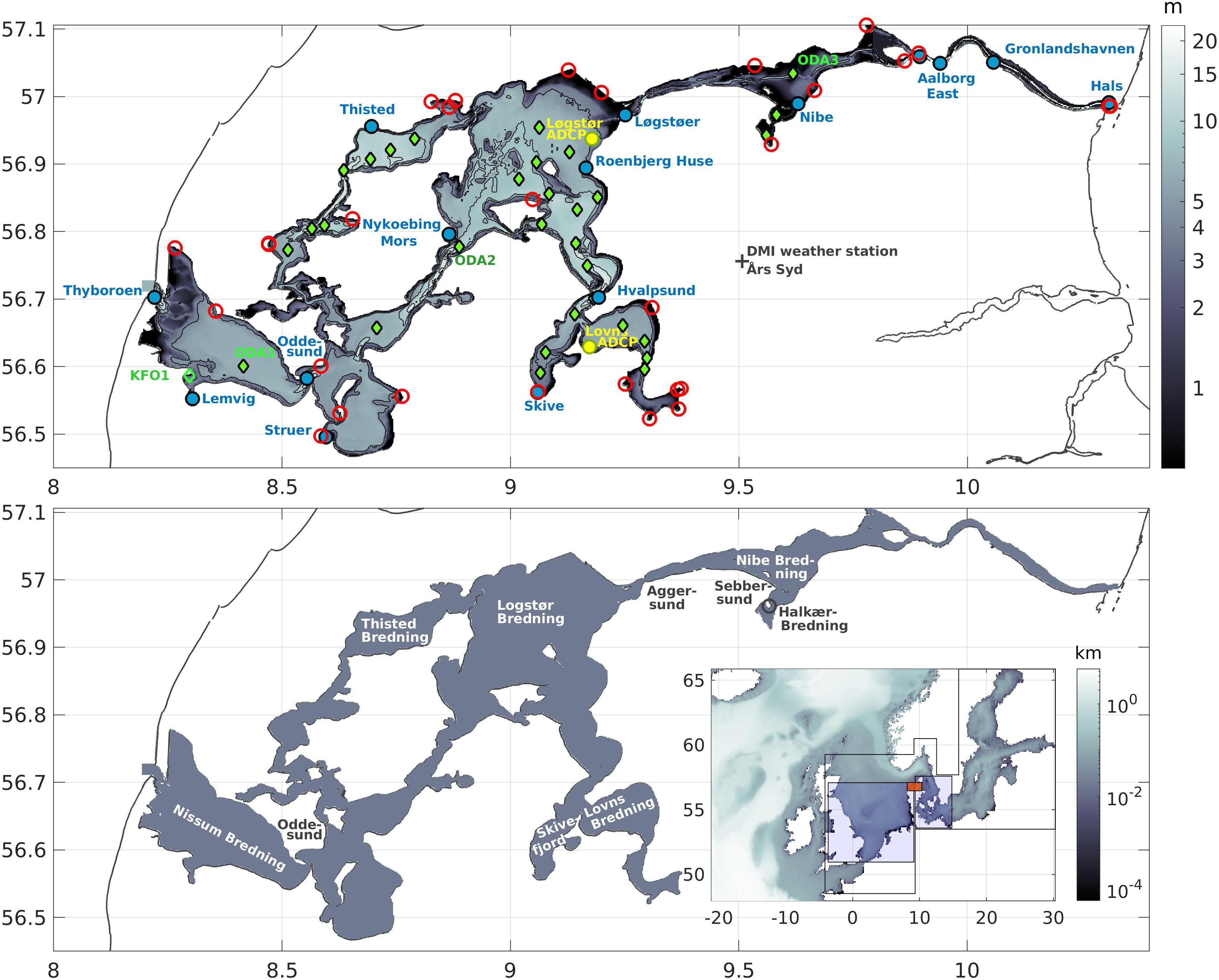
Figure 1. HBM Limfjord model setup in 185.2 m resolution. Markers indicate the locations of the tide gauge stations (blue circles and names), ADCP current measurement stations Lovns and Løgstør (yellow dots), salinity and temperature validation stations (green diamonds) and river locations (red circles). Inset figure: Model configuration with a spatial resolution of 3 nmi in the North Sea and Baltic Sea, 1nm in the Waddensea, 0.5 nmi in the Danish straits and 185.2 m resolution in the Limfjord domain (red box).

The local, wind condition are characterized by predominantly zonal, westerly winds, which accounts for more than 50% of all configurations, with some year-to-year variations. While westerly winds are typical of autumn and winter, easterly winds are less frequent and occur mainly in summer periods. The wind velocity follows a Weibull distribution, centered at 6 m/s, and ranging up to values of 38 m/s, for strong storms (Christiansen et al., 2006).

The main water transport is eastward, from the North Sea to the Kattegat, driven mainly by the westerly winds over the North Sea and the Limfjord as well as the sea level boundary conditions in Thyboron and Hals. The fjord hydrography is characterized by a strong zonal salinity gradient with salinities in the range 32–34 psu at the western opening to the North Sea and 19–25 psu at the narrow outlet to the Kattegat (Maar et al., 2010). Freshwater runoff of 2.6–2.7 km³/year is one of the factors that controls the salinity dynamic in the fjord (Thodsen et al., 2018). About 34% of the fjord’s volume is replaced by river runoff every year. Some parts of the fjord are very brackish and can freeze over during severe winter. The average water temperature in the fjord is about 2–3°C in winter and 15–17°C in summer (Wiles et al., 2006). Currents, mixing and stratification in Limfjord are mainly driven by wind induced mixing and density changes (Hofmeister et al., 2009). Recent measurements in different broads of the Limfjord indicated rapidly changing currents of both magnitude and direction over the course of hours to days (Pastor et al., 2020). Model simulations by Pastor et al. (2021) predict the strongest time-averaged currents and highest variability of current velocities across the fjord at the western boundary in Nissum Bredning and inside narrow channels connecting the broads further east. In these areas, mean currents of up to 10 and 20 cm s^–1 were reported in May/June 2010, whereas currents inside the larger broads did not exceed 5 cm s^–1 during the same period (Pastor et al., 2021).

The Limfjord is of great importance for local communities due to its large ecosystem services and recreational value. The fjord supports a high biomass of benthic suspension feeders dominated by a natural population of blue mussel (Mytilus edulis) sustaining a substantial mussel fisheries industry (Frandsen et al., 2015). The Limfjord is also an important area for protection of eelgrass beds (Zostera marina)–a key indicator species under the European Water Framework Directive (WFD-EU, 2009). Thus, safeguarding the presence and recovery of eelgrass beds in protected areas of the fjord is a central aspect of local marine management efforts (Krause-Jensen et al., 2005). Part of the management strategies involve a coordinated effort of mussel fishing and eelgrass protection interests to limit possible effects of suspended sediment plumes from mussel dredging on light conditions for seagrasses (Holmer et al., 2003; Pastor et al., 2020). The implementation of local or fjord wide management plans such as the delineation of fixed buffer zones around mussel dredging areas requires information of local environmental conditions on fine temporal and spatial scales. However, narrow estuaries, inlets and fjords are often not covered by EU operational oceanographic products from e.g., Copernicus Marine Environment Service (CMEMS). To support coastal zone management efforts on a national and community level, seamless operational modeling capacity will have to be developed to resolve coastal-estuary continuum (She and Murawski, 2018).

Previous modeling efforts in the Limfjord involved mechanistic models for a variety of management and research applications. The modeling studies investigated the functioning and dynamics of benthic filter feeders (e.g., Maar et al., 2010), estimated the effects of mussel fishing activities on the sediment dynamics (Holmer et al., 2003; Pastor et al., 2020), studied the species connectivity (Pastor et al., 2021) and investigated physical drivers of stratification and de-stratification (Wiles et al., 2006; Hofmeister et al., 2009). Other modeling applications were dedicated to estimate changes in the frequency and magnitude of storm surges and water levels as a consequence of climate change (Knudsen et al., 2012). Hofmeister et al. (2009) investigated the hydrodynamics in the Limfjord using the General Estuary Transport Model (GETM). The model was applied as a stand-alone setup by using observed river discharges and observed sea level, water temperature and salinity as lateral boundary conditions in the North Sea and Kattegat. Pastor et al. (2021) used a 3D physical model system (FlexSem; Larsen et al., 2020) coupled to an agent-based model to study dispersal and settling of mussel larvae between 17 areas in the Limfjord.

Operational models provide a good platform for assessing ocean conditions, as they are not specifically tuned to certain processes and scenarios, but rather provide a good overall performance for a number of user applications. They are extensively validated to provide reliable community services in coastal and open waters including storm surge and temperature forecasting. DMI’s operational forecasting service for the Limfjord was established in 2007 for the purpose of storm surge warnings. At that time it was decided to abandon the older 2D models and to apply the operational storm surge model: HIROMB-BOOS Model (HBM) to the Limfjord in a horizontal resolution of 370.4 m (12″× 20″). The set-up was extensively tuned and has provided a good quality service since then. However, a fully two-way nested model system could not be established, as the model resolution in the surrounding seas was too low, at the time. Adequate river runoff was not available, so that the forecasting system could not address issues with the forecast quality of salinity, water temperature, stratification and sea ice.

The recent need for these parameters for coastal aquaculture support has sparked new model developments as part of two recent national and international research initiatives, TASSEEF and FORCOAST, dedicated to the management of the coastal zone in Danish and European waters. The main goal of the TASSEEF project was to develop new tools and methods for estimating the environmental impacts of mussel fishing in the Limfjord, in particular the generation and propagation of sediment plumes from mussel dredging (Pastor et al., 2020). The EU H2020 FORCOAST aims to develop novel CMEMS-based downstream services in different case study areas along European coastal zones including the Limfjord. In this study, we introduce a high-resolution implementation of the three-dimension (3D) HBM ocean model for the Limfjord. We highlight its potential benefit for both local coastal zone management questions in Danish waters and for contributing to the CMEMS data portfolio as new category of high-resolution data products in strategically important coastal areas.

This paper is organized as follows: section “Model Description” introduces the physical and numerical basis of the HBM ocean circulation model. Section “Model Configuration and Set-Up” continues with the model setup and configurations for the simulation experiments and section “Model Validation Data Set” describes the observation datasets. Section “HBM Application for the Coastal Zone” demonstrates the ability of the model to provide reliable, high quality forecasts, for sea level predictions and coastal management applications. This section is devoted to a service oriented analysis of the model performance for storm surge warnings, ocean forecasts for aquafarming support and the coastal management of mussel fishery impacts. Section “Discussion and Conclusion” discusses the results and derives conclusions for the application of ocean circulation model to the coastal zones.

Model Description

The HBM model is a 3D, baroclinic ocean circulation and sea ice model suitable for the shelf-sea and coastal dynamics. The model is set-up to cover the North Sea and Baltic Sea, but has been extended to resolve coastal, estuary scales: Elbe estuary and fjords: Lillebaelt, Roskilde Fjord and the Limfjord as well. Originally developed in the 1990’s at the Federal Agency for Sea Shipping and Hydrography (BSH) in Hamburg (as BSHcmod, Dick et al., 2001), the HBM model has been continuously developed as a national operational forecasting system in Denmark and Germany since then and has been used as CMEMS BAL MFC forecasting system since 2008–2020 (Poulsen and Berg, 2012; BalMFC Group, 2014). The model is implemented with dynamic two-way nesting in 3D space and time, as well as flooding and drying in shallow waters and tidal flats, allowing to set-up models with different demands for spatial and temporal resolution in shallow coastal waters which may fall dry due to low tides and offshore winds.

Dynamic two-way nesting allows for frequent exchange of mass and momentum between coarse and fine grids. The method uses the hydrodynamic solver and tracer-flow-routines, to calculate the dynamics at the interface. Fine-to-coarse grid nesting applies grid cell volume averages of scalars (salinity, temperature, etc.) and grid cell interface averages of currents, to determine the transport into the coarse grid cell, whereas coarse-to-fine nesting uses the area-or volume fraction of the fine grid cell to determine the transport into the fine grid cell. Nesting takes place every coarse grid time-step, which must be sub-dividable into fine grid steps.

HBM solves the dynamic equations for momentum and mass, and budget equations for salinity, heat and other tracers, on a spherical grid with a number of model levels at fixed depths in the vertical dimension. The free surface implementation allows for varying sea level and the flooding and drying of grid cells. The horizontal advection and diffusion is modeled using a flux corrected transport scheme. The Boussinesq approximation is applied. In the vertical direction, the model assumes hydrostatic balance and incompressibility of sea water. Higher order contributions to the dynamics are parameterized following Smagorinsky (1963) in the horizontal direction and a k-ω turbulence closure scheme, which has been extended for buoyancy-affected geophysical flows in the vertical direction (Berg, 2012). The turbulence model includes a parameterization of breaking surface waves (Craig and Banner, 1994) and internal waves (Axell, 2002). Stability functions from Canuto et al. (2002, 2010) for the vertical eddy diffusivities of salinity, temperature and momentum are applied. Additionally, the turbulence closure scheme considers realizability criteria (Brüning, 2020), to ensure the numerical stability of the model. HBM includes a thermodynamic and sea ice model, which describes the dynamic of free drifting ice and coastal fast ice. For more information on HBM the reader is referred to Berg and Poulsen (2012), Poulsen and Berg (2012), and BalMFC Group (2014).

Benefitted from its high performance computing efficiency and flexible grid with dynamic two-way nesting, the HBM development has been oriented toward seamless model applications from basin-scale to coastal and estuary scales that can be operated with the same executable (She and Murawski, 2018). Site and application specific tunings have been kept at a minimum. This has benefitted the general performance of the model, as the trend has been to increase model resolution and the coverage of coastal high-resolution model domains. Operating the model in high vertical resolution and in wind sheltered environments, typical for estuary and fjord models required an update of the shear-production of turbulence near the surface, to ensure a homogeneous profile of the vertical diffusivities (for momentum, heat, and salt). Entirely wind dependent boundary conditions, following Craig and Banner (1994) might underestimate the surface production of turbulence and mixing in wind sheltered environments. Therefore, shear and buoyancy production of turbulent kinetic energy k and dissipation rate ω was enhanced and added to the surface production of turbulence through the breaking of surface wave (Berg, 2012). A scaling factor was introduced, to increase the surface shear production of turbulent kinetic energy, which in the model, is limited by the vertical resolution of the model grid. Vertical shear of surface currents is calculated at the interface between the surface and sub-surface layer, which in the Limfjord domain is at 2 m depth. It has been found that increasing surface production is beneficial for the modeling of homogeneous current profiles in the shallow regions of the Limfjord.

The increase in vertical resolution required also the implementation of flux-boundary conditions for the sensible and latent heat exchange at the ocean-atmosphere interface, instead of the previously used bulk formulations, which tended to cool down to fast in winter. The current implementation uses a blend of Kara et al. (2005) and the COARE 3.0 algorithm (Fairall et al., 2003), which transfers the 2 m air temperatures to 10 m values.

It is a challenge to simulate temperature in very shallow waters as bottom soil becomes an integrated part of vertical heat exchange. The current version of HBM uses a soil heat transport model which simulates the heat exchange between the lowest model layer and the soil sediments. In very shallow water, the HBM model used to under-predict water temperature, as the fraction of the solar radiation that was reaching the ground was neither reflected back nor used to heat the sea bed, but was neglected. This led to an under-prediction of water temperature in shallow estuaries. In the current implementation, this was remedied by increasing the light absorption near the surface due to a linear, depth dependent scaling in very shallow waters. HBM uses a two-band, short- and longwave radiation model for the intensity of the solar radiation, following Meier, 2001. The two bands have different extinction lengths: ζ_LW = 3.26 m for the longwave radiation and ζ_SW = 1.78 m for the shortwave radiation. The shallow water radiation model reduces the extinction length of the short wave radiation in shallow waters, with depth lower than H_max = 5 m, by applying the linear scaling ζ_SW = 1.78 m ⋅ max(0.2, h/H_max), with h being the depth of the model layer. With this formulation, up to 94% of the short wave radiation in shallow waters is absorbed in the upper 1 m of the water column.

Seamless model applications that zoom in onto coastal and estuary scales are comprehensive and require high computational efficiency to reach the required performance. In the case of HBM this has been approached by increasing the degree of parallel computing efficiency of the code. The model has been developed for using multi-core and many core supercomputers with hybrid parallelization performance (Poulsen et al., 2015). Furthermore, the memory efficiency was improved, by using Non-Uniform-Memory-Access (NUMA) together with a “first touch” of the memory during initialization in order to enhance the locality of the memory in relation to the CPU (Poulsen et al., 2015). Domain decomposition using hybrid OpenMP + MPI parallelization was accomplished through load-balancing of the computation, i.e., by distributing sub-slices of the grid in such a way, that each MPI domain holds nearly an equal share of the number of wet-point of the entire grid. Dealing with an extensive number of wet-points requires the implementation of an io-server, which can handle the larger amount of data and can perform input/output in parallel to the computation. HBM is using an asynchronous io-server that permits other tasks to continue their computation. These elements together allow it to run very memory demanding applications. The execution of the two-way nested North Sea, Baltic Sea and Limfjord set-up takes about 2.5 min per simulated day, using 144 cores on DMI’s current HPC Cray-XC development cluster.

Model Configuration and Set-Up

The seamless, two-way nested HBM model set-up covers 5 domains (Figure 1, inset): the North Sea and Baltic Sea in 3 nautical mile (nmi) horizontal resolution, the Wadden Sea/West Coast and the Danish Straits in in 1.0 and 0.5 nmi resolution, and the Limfjord in 185.2 m (1/10-th of a nautical mile) resolution, nested in between the extended Waddensea domain and the Danish Straits (Table 1). The Limfjord set-up has been nested into DMI’s operational storm-surge set-up, to ensure the good quality of the water level signals propagating into the Limfjord. The vertical grid uses a surface layer of 2 m thickness, to include the range of wind and tidal driven sea level variations and a maximum of 22 sub-surface layers, covering the depth range of up to 28 m at Oddesund. The 2 m thickness of the surface layer is required, to prevent it from falling dry in cases of exceedingly low sea levels, at locations with more than just one model layers. Below the surface, the layer thickness is 1 m, but it can vary near the sea bed, to take bathymetric changes into consideration. The layer structure in the two-way nested Limfjord domain represents a refinement of the corresponding layer structure in the two parent domains: the Waddensea and the Danish Straits. The surface layer thickness in the Waddensea features a thickness 4 m, to handle the larger tidal range. Below the surface, the thickness is slowly increasing, from 2 m in the upper 80 to 50 m at a depth of 250 m. The layer structure in the Danish Straits domain is identical to the one in the Limfjord domain, in the upper 30 m. Below that, the thickness is increasing to 2 m, down to a depth of 76 m in the Danish Straits and 700 m in the Skagerak and the North Sea. At the open model boundaries in the English Chanel and toward the North Atlantic, connecting the Orkneys to the coast of Norway (Figure 1), the model is using tidal sea surface elevations based on 17 constituents and pre-calculated surges from a 2D barotropic model covering the North Atlantic. Barotropic currents that are in balance with the sea surface slope are imposed on the outside of the open model boundaries. The model is using climatological boundary conditions for salinity and temperature buffered by a sponge layer.

TABLE 1

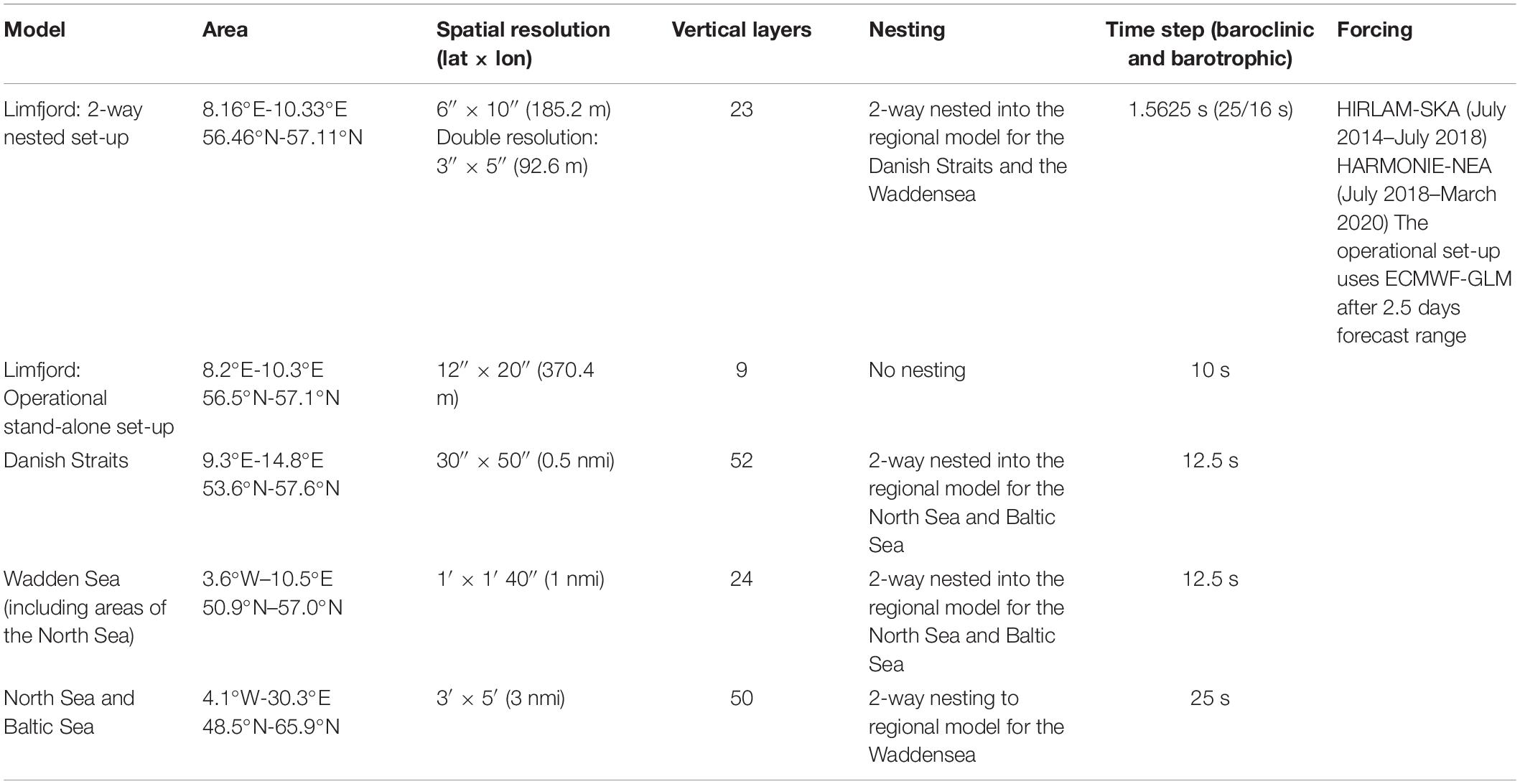
Table 1. Overview over the HBM model setup.

Meteorological forcing is from DMI’s operational high resolution numerical weather prediction model, first the hydrostatic HIRLAM model in 3 km resolution, until July 2018, and then non-hydrostatic HARMONIE model in 2.5 km resolution. Daily river runoff data from the Swedish E-Hype3 model (Donnelly et al., 2016) is applied at 662 inflow locations, of which 30 are located in the Limfjord (Figure 1, red circles). The 5 year hind-cast model run was initialized in July 2014 using observations from the national environmental monitoring program NOVANA, made available by the Danish Center for Environment DCE at the Aarhus University in collaboration with the Danish Ministry for Environment and Food: Overfladenvandsdatabasen ODA¹. Outside the Limfjord, salinity and temperature fields from DMI’s operational storm surge model were used for initialization. The model started from a configuration of zero currents and sea level and run first for a 6 month spin-up period, from July to December 2014, followed by a 5 + year hind-cast period, until March 2020, to produce the data set for the analysis.

DMI’s operational storm surge forecasting system uses a single domain, stand-alone Limfjord model, covering the same model domain as the nested setup (Figure 1), in half the horizontal resolution 370.4 m and a lower vertical resolution of 2 m at all model layers. In this study, the stand-alone model is used as a reference model for the storm surge assessments. The boundary conditions for sea level, salinity and temperature are provided by DMI’s operational North Sea and Baltic Sea model, featuring a horizontal model resolution of 6 nmi in the North Sea and 0.5 nmi in the Kattegat and the Danish Straits. The operational model runs 4 times per day, for a 5 day forecast, using high resolution meteorological forcing from DMI’s operational limited area weather prediction model for the first 2.5 days and coarser, global ECMWF-GLM forcing thereafter. In this study we use only the model data from the first 6 h of each run.

Model Validation Data Set

Extensive model validation has been performed to assess the quality of the model and to quantify the confidence limits of its predictions, thereby defining the applicability of the model and the set-up. This paper looks into two types of validation studies: long-term validation of sea level, salinity and temperature, using monitoring data from operational data collection and aggregation programs and short-term validation studies using observations from national and EU projects, which were collected over a limited period of time (Table 2).

TABLE 2

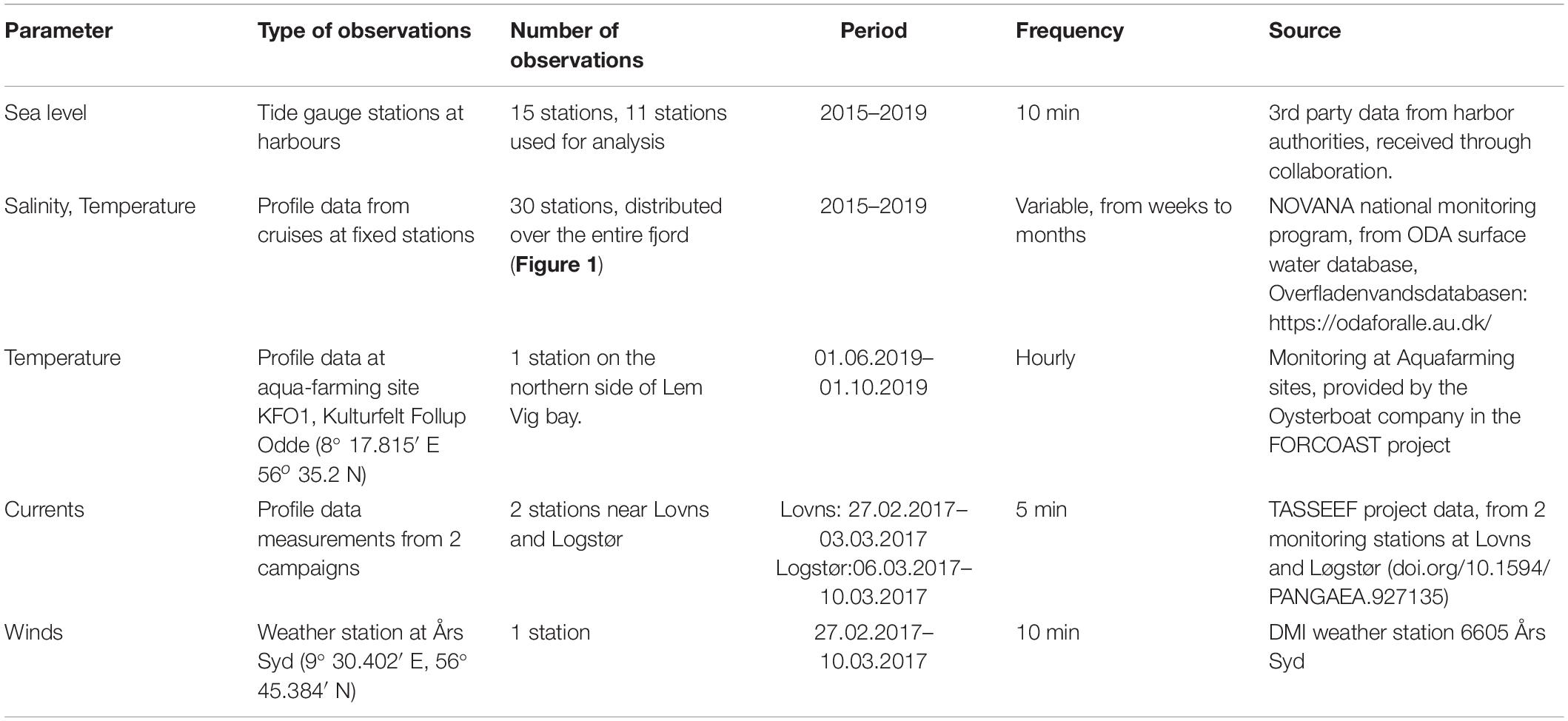
Table 2. List of data sets used for model validation.

Denmark has a dense network of sea level monitoring stations. The Limfjord alone is covered by 15 stations, which are operated by local harbor authorities and provided to DMI in real-time. 11 of these stations were selected for statistical analysis (Table 2).

Salinity and temperature profiles from NOVANA national environmental monitoring program cruises have been made available by the Danish Center for Environment DCE at the Aarhus University, in collaboration with the Danish Ministry for Environment and Food. Time range and frequency of the observations are variable and change from station to station.

High frequency (hourly) temperature data from a shallow water monitoring station KFO1 at aquafarming site: Kulturfelt Follup Odde, near Lemvig has been provided by the Oysterboat Company, in the FORCOAST project. The depth of the bottom sensor was approximately 2.3 m, 20 cm above the seabed. The model depth at the site is only 1.4 m. The sensor was deployed on the 3rd of June 2019 and recovered on the 1th of October 2019.

ADCP observations of currents at two mussel dredging sites near Lovns and Løgstør have been collected during two measurement campaigns in spring 2017, as part of the TASSEEF project. The two deployments covered 5 days (27th February–3th March 2017, Lovns Bredning; 6th–10th March 2017, Løgstør Bredning), using a 600 kHz ADCP (RDI Workhorse Sentinel) as part of a larger mooring array (Pastor et al., 2020). The ADCP was deployed in a bottom-mounted, upward-looking configuration and recorded ensemble averaged profiles of 3D current velocities every 30 s. The vertical bin size was set to of 0.5 m and the first bin was collected at 1.59 m above the bottom (blanking distance: 0.88 m). The time series were filtered using 30 min moving average.

HBM Application for the Coastal Zone

This section analyses results of using the model system for storm surge prediction and marine resource information service applications, which require seamless, high resolution model data and forecasts for the coastal zone. The performance of the Limfjord model with regards to predicting sea level, currents, temperature and salinity distribution are evaluated across the fjord.

Operational Storm Surge Forecasting Service

Denmark is frequently exposed to storm surges, generated by strong, predominantly westerly winds that raise the waters along the west coast and produce sea level gradients in the Baltic Sea, which in their turn can lead to strong seiches later on, when the winds abate and the balancing movement returns the water to its original level. Highest recorded sea level in Denmark occurred during storm surges in the North Sea, with the record being the October storm 1634, with up to 6.34 m above Danish Normal Null in the inner part of the German Bight. Wind driven sea level variations in the Limfjord can be strong in the storm cases (Knudsen et al., 2012). In the years following 1960, modeled sea level maxima exceeded well beyond 2.5 m in northern Jutland, at the western entrance to the Limfjord, near Thyborøn. In open waters and near the entrance to the western Limfjord, modeled sea levels rarely exceed 1.6–1.7 m. Even though the sea level maxima did not occur at the same time, it is clear that predominantly westerly winds generate east-western sea level gradients in the fjord. The balancing water transport through the fjord, together with the limited capacity for transport through the narrow straits of the fjord, leads to local sea level maxima inside the fjord that can exceed the values at the North Sea entrance, and has reached values up to 2.1 m. Sea level maxima inside the fjord have continuously increased, since 1825, when the North Sea entrance was established, due to a continuous, erosive widening of Thyboron channel, through tidal currents and wind driven currents associated with storm events.

The Limfjord is divided into a western and eastern part, as is demonstrated by the correlations of the observed sea levels with the boundary signal at the entrance stations Thyboron and Hals (Figure 2). The western side of the fjord extends roughly from Thyboron (a) to Haverslef Havn (i), while the eastern side covers the stations from Aalborg (j) to Hals (l). This is advantageous for the setting up a stand-alone model set-up, as the tuning of the boundary signal at the two entrances is rather independent of each other. In this study, we compare the nested, high resolution set-up in 185.2 m (6″× 10″) resolution with DMI’s operational, stand-alone model set-up in half the resolution, 370.4 m (12″× 20″).

FIGURE 2

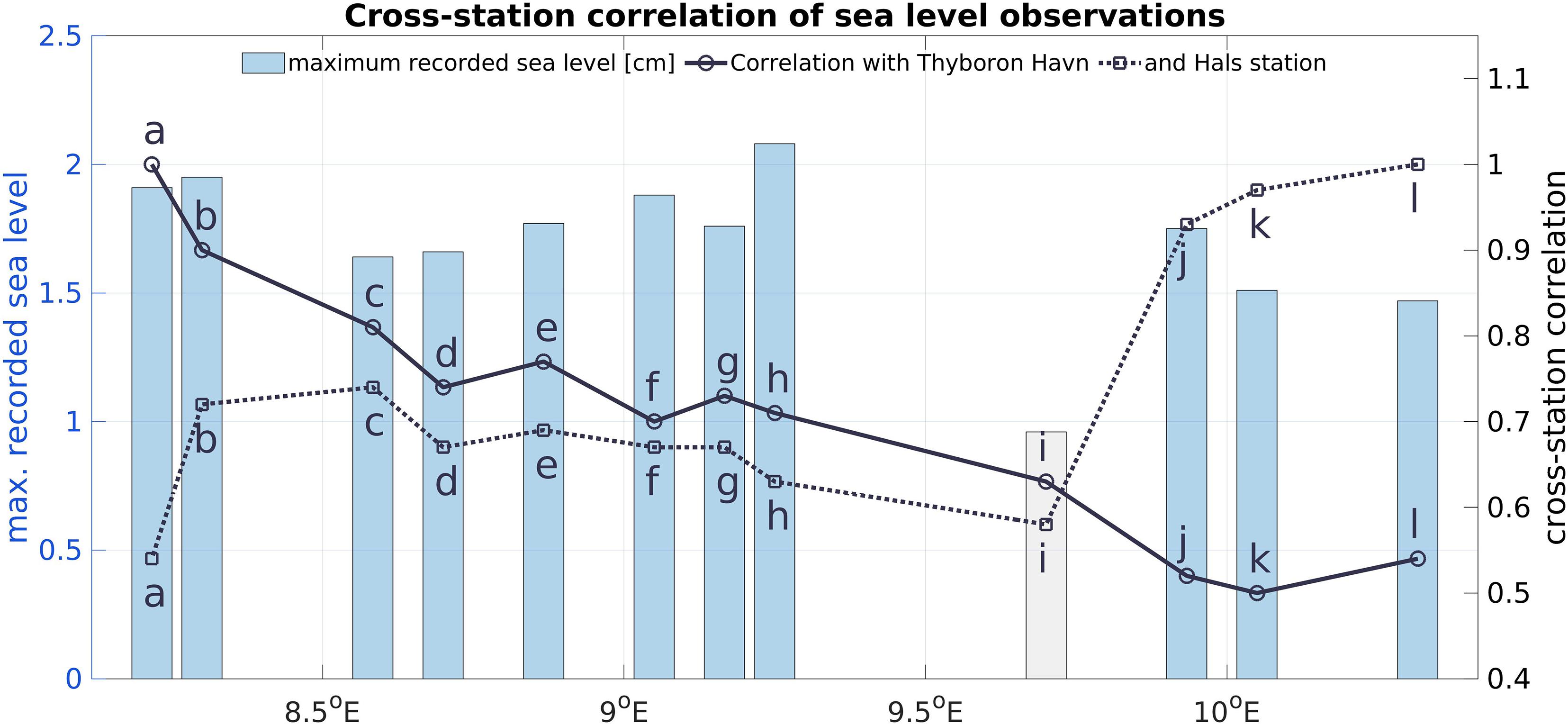
Figure 2. Maximum recorded sea level at Limfjord stations (bars) and cross-station correlation coefficient (lines) of observed sea levels with the sea levels at the boundary stations Thyboron (full lines) and Hals (dotted lines). From west-to-east: (a) Thyboron, (b) Lemvig, (c) Struer, (d) Thisted, (e) Nykøbing Mors, (f) Skive, (g) Rønbjerg Huse, (h) Logstør, (i) Haverslev Havn, (j) Aalborg East, (k) Grønlandshavn and (l) Hals. Haverslev is a new station, which has been established in 2017.

The operational set-up has been tuned extensively and has provided a reliable storm surge warning service for many years. It has been set-up in such a way, that the boundary tuning is slightly compromising the stations near the eastern boundaries, in order to benefit the ones in the interior of the fjord, especially Aalborg, which is Denmark’s fourth largest city and one of its biggest shipping harbors. The west-to-east water transport through the fjord has been enhanced by adding 10 cm to the western and −15 cm to the eastern boundary signal, as well as intensifying the signal by 10 percent. This has largely reduced the sea level bias near Aalborg in the east of the fjord (Figure 3), i.e., the difference between the mean of the model time series and the mean of the observed time series. But biases are usually not in the focus of the model quality assessment, because they are relatively easy to correct. They have been added here, to demonstrate the effect of the boundary tuning, whose main purpose is to reduce the absolute error, i.e., the cRMSE (centered Root Mean Square Error), the RMSE of the de-biased time series and the phase error. It should also be mentioned, that boundary tuning is only one aspect of model set-up development. Most work is actually spent on tuning the model bathymetry, with focus on the correct implementation of bathymetric features, e.g., drying out depth, sub-surface channels, trenches and sills, etc., which has to be carried out for each set-up individually. Comparing DMI’s operational stand-alone setup with the fully two-way nested set-up, the advantages and disadvantages of the two approaches can be studied. The possibility to improve the model performance through boundary tuning makes it possible to adapt the stand-alone model more easily to the conditions at a given site, e.g., Aalborg harbor and to provide a good service for where it is needed. This, however, may come at the expense of the model performance at other sites, as the cRMSE values demonstrate. The two-way nested set-up has lower cRMSE values nearly everywhere in the entire fjord, except for Aalborg, which is the station for which the stand-alone set-up was mainly tuned. This is reflected in the average cRMSE’s for the two-way nested and operational stand-alone model setup, respectively, which at western Limfjord stations is 8.4 cm/10.4 cm, at central stations is 6.7 cm/8.2 cm and at eastern stations is 9.24 cm/9.3 cm. The comparison (Figure 3) shows, that the two-way nested set-up has a superior overall performance, whereas the stand-alone set-up has the best targeted performance.

FIGURE 3

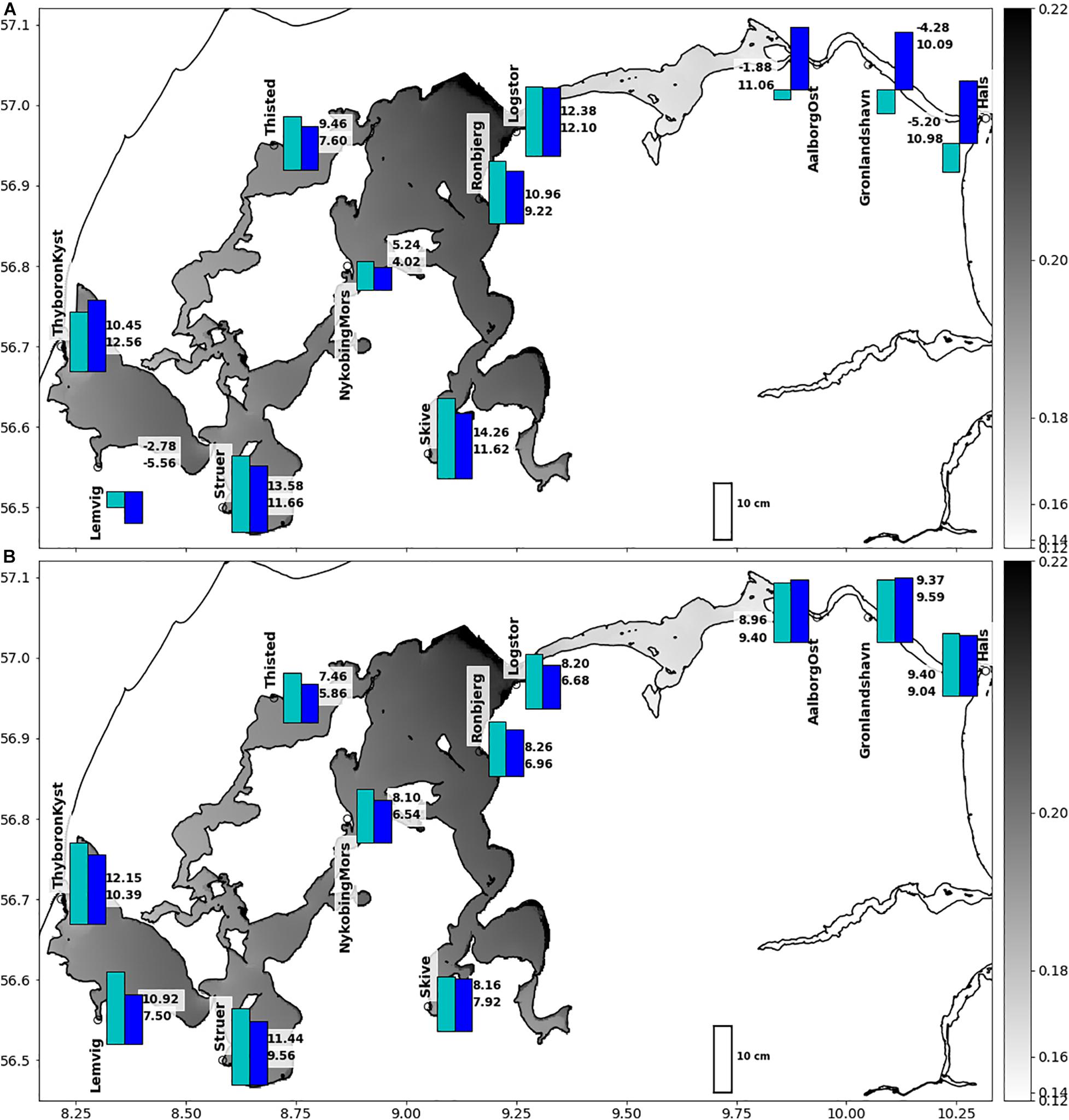
Figure 3. Bias (A) and centered Root-Mean-Square-Error (cRMSE) (B) of DMI’s operational stand-alone model (light blue, upper number) and two-way nested model (dark blue, lower number). Units are given in centimeter. The shading shows the modeled 5 year mean sea-level. Restricted water transport through narrows at Oddesund (near Struer) and Agersund (near Løgstør) leads to a higher mean sea level in the western part of the fjord.

Model quality assessments use statistical evaluations of long-term sea level data to provide a general overview of the model performance, but they focus on skill scores, to analyze the model performance from a service point of view. Skill scores provide robust quality measures for the annual assessment of the 10 highest measured and modeled sea level events. Usually the analysis refers to a storm season: September–April, but for the analysis in this paper, the assessment period has been shifted, to cover one calendar year instead. Currently, the metrics focuses on the magnitudes of the events, but new metrics are under development, which look deeper into the capacity of the models to predict the timing of the events as well. This has gained importance in recent years, due to an increased focus on the efficient management of mobile countermeasures, i.e., moveable sea walls.

Skill assessments study the percentages of successful forecasts within a given period of time, here 5 years. Focusing on the 10 highest, observed sea level events, the peak-error, i.e., the absolute difference of modeled and observed peak value, is evaluated against tolerance limits, which are defined as 10% of the observed sea level peak, with a lower limit of at least 10 cm. Double-tolerance-assessments use a minimum value of ± 20 cm. The forecast is counted a “miss,” if this range is exceeded; otherwise it is counted a “hit.” Finally, miss-rates are calculated and reported. The assessment neglects phase errors by allowing for a time shift of up to ± 6 h between modeled and observed peak. The method identifies the maximum of the modeled time series within a 12 h search window that is centered at the time of the peak observation. A peak separation time of 12 h, roughly one tidal period, is implemented, to two avoid double-counting individual peak events.

For peak error, absolute peak error and peak miss rate, the two-way nested model (Figure 4A) is superior to the stand-alone model (Figure 4B) at all stations. The geographical distribution of high, absolute peak-errors and miss-rates shows a strong dependency on the progressing speed of the sea level signal through narrow trenches, especially through Oddesund, near Struer (Figure 4c), through Aggersund, near Rønbjerg Huse (Figure 4g) and through Aalborg, at Aalborg East (Figure 4j). This is a common problem of many fjord set-ups, and a problem that is difficult to solve with coarse resolution models. The correct timing of the events depends on the transport capacity of the sounds, i.e., the depth and width of its narrowest parts, which needs to be resolved in adequate resolution. Blocking effects play a role as well, especially for the central Limfjord stations: Logstør and Rønbjerg Huse (Figures 4g,h), whose water levels depend on the blocking of the westwards transport of water at Feggesund, north of the island of Mors.

FIGURE 4

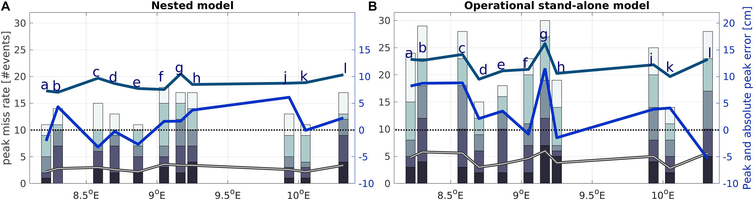
Figure 4. Peak-error comparison of nested model set-up (A) and operational stand alone set-up (B). Peak error (light blue), absolute peak error (dark blue) of single tolerance assessments and sum of missed peak events (grey) 2015–2019: annual values (bar diagram) and mean value (line), for sea level stations, from west-to-east: (a) Thyboron, (b) Lemvig, (c) Struer, (d) Thisted, (e) Nykøbing Mors, (f) Skive, (g) Rønbjerg Huse, (h) Logstør, (j) Aalborg East, (k) Grønlandshavn and (l) Hals.

From a service point of view, it makes sense to distinguish between an under-prediction and an over-prediction of a peak event, and to penalize the model stronger for an under-prediction, which might lead to a missed warning. This has been the tuning strategy for the current operational system (Figure 4B), which enhances the transport through the fjord by tilting and amplifying the boundary signal by adding 10 cm to the mean sea level in the west and subtracting 15 cm in the east, as well as amplifying both by 10%. The development of an operational model configuration is quite comprehensive and involves the tuning of the model parameter, bathymetry and boundary conditions for storm scenarios and long-term simulations. This is usually done in steps, so that first the bathymetry is established and then tested using different boundary conditions. The sea level boundary tuning improves the barotropic flow at the open model boundary and the water transport through the narrow straits of the Limfjord, with positive consequences for the quality of the sea level forecast. The current operational stand-alone configuration has been tuned especially, to avoid missed warnings in the central Limfjord and in Aalborg. The downside of this approach is that it leads to a general over-prediction of the sea level peak events, which is reflected in the higher peak errors and miss rates, especially near the boundaries. The nested set-up is clearly better in predicting peak events, i.e., storm surges, but it also tends to under-predict some of the peaks at Struer and Nykøbing Mors (Figures 4c,e), leading to missed warnings. Further work is needed to develop the bathymetry of the two-way nested Limfjord set-up to a level where it can be used for operational storm surge predictions.

Comparing the two types of operational models that might be developed for a local area application: i.e., the fully two-way nested model and the stand-alone model, it is apparent that stand-alone-models are useful for targeted operations at given sites, whereas the nested models are better in providing operational services for the entire model domain. The option of tuning the boundary conditions makes stand-alone model more adaptable to the local conditions. At Aalborg East, the cRMSE of the stand-alone model is with 8.96 cm smaller than the cRMSE of the two-way nested set-up 9.4 cm, while the absolute peak error is larger: 9.6 cm in comparison to 6 cm for the two-way nested set-up. However, this comes at the expense of the model performance at other sites, which are not part of the tuning. For a user with given interest in a specific site, it makes sense to set-up a stand-alone models using boundary conditions that are provided by CMEMS or other service providers. For a general service provider like CMEMS, however, it is more feasible to extend the service and to develop, high-resolution, nested coastal and estuary applications. Both approaches can be developed, by employing local-area, stand-alone models from local providers to develop downstream services for interested users, and by further enhancing the CMEMS modeling capacity to include coastal end estuary scales using nested models.

Ocean Physical and Ecological Services for Aquaculture Support

Hydrographic conditions are essential for aqua-farming, such as oyster and blue mussel farming, in Limfjord. On one hand, the aquaculture species have preferred water temperature and salinity for their growth. On the other hand, stratification can affect oxygen and food status for the oyster and blue mussels. It was found, that the strength of stratification determines, in part, the estuary’s sensitivity toward oxygen depletion (Christiansen et al., 2006). In well-mixed water mussels are capable of depleting the whole water column while for stratified water the food supply will be limited, thus may act as a temporary refuge for phytoplankton, allowing the population to recover (Wiles et al., 2006).

Aquafarming in the Limfjord involves oyster cultivation of Ostrea edulis in the western part of the fjord. The farming process involves the moving of the oysers to seawater sites (Kulturfelt) after they have passed the nursery phase. Some of these sites are situated in very shallow waters with model depth of little more than 1 m. A good model quality with regards to temperature predictions in shallow water is therefore critical for the farming operation. In this study it was found that the original HBM model under-estimate the shallow water temperature significantly, as shown in Figure 5 (blue line) when comparing with hourly water temperature observations at station KFO1. The sub-surface radiation scheme of the HBM model was then adapted to very shallow waters, to overcome the cold bias of the previous model version (Figure 5). This led to a stronger absorption of the short wave radiation near the surface and to a significant decrease of the temperature bias from −1.39 to −0.48°C. The diurnal variability was enhanced, leading to lower cRMSE’s of 0.43°C, instead of 0.58°C in the previous model version.

FIGURE 5

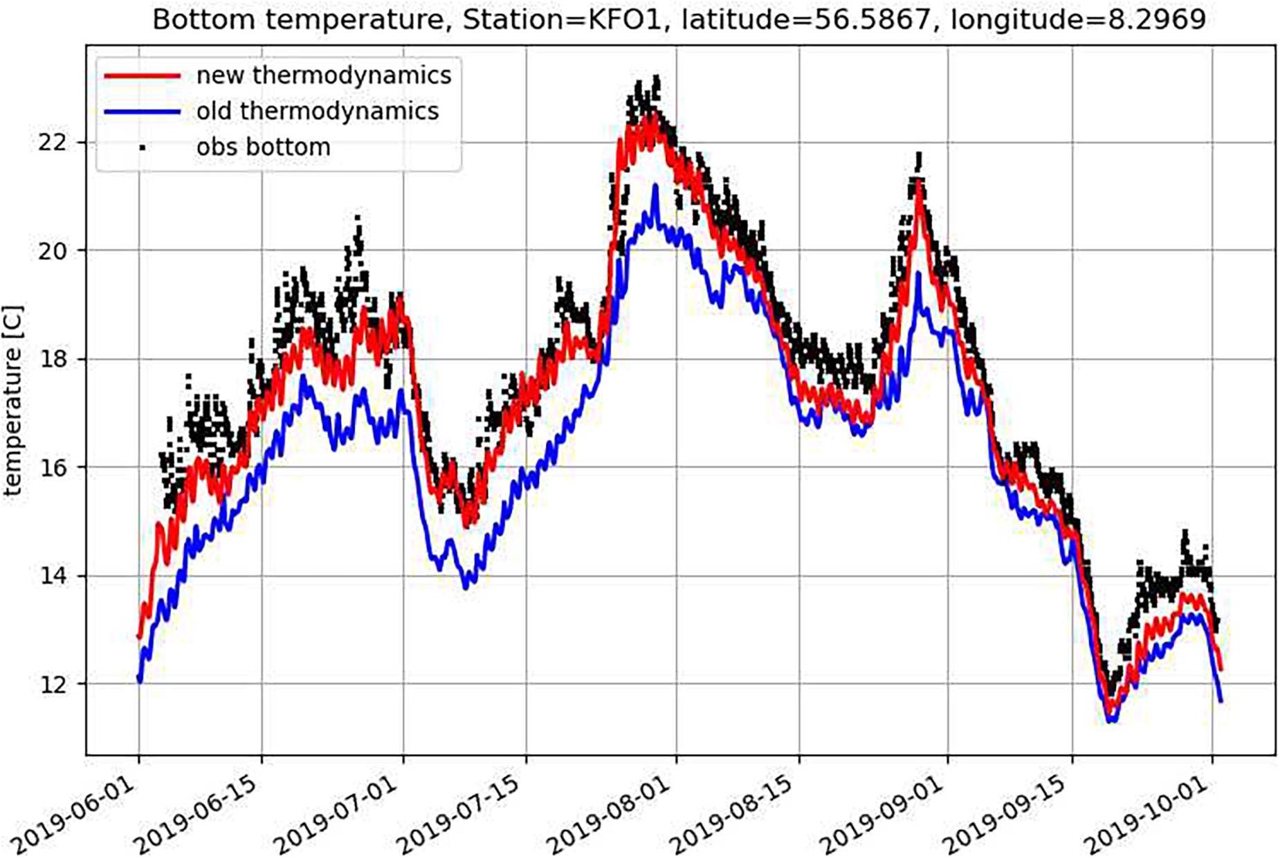
Figure 5. Impacts of the shallow water radiation scheme on the HBM model prediction of near surface temperature: Observations (black dotted), model with previous surface radiation scheme (blue) and improved surface radiation scheme (red).

Modeling Horizontal Patterns of Temperature and Salinity

The physical environment of the Limfjord is very dynamic and characterized by a fast and efficient water mass renewal process, controlled by wind forcing, lateral boundary conditions and river runoff. The volume of the shallow fjord is small enough (7.72 km³) for river runoff to amount for an annual water mass renewal rate of about 34% of the fjords volume. The water exchange with the North Sea and the Kattegat adds to these numbers. Saline North Sea water enters the fjord through Thyborøn Channel and is transported eastward. Occasionally less saline water can enter from the Kattegat side and flow westwards. There are quite a number of narrow passages in the fjord, e.g., Oddesunde and Aggersund, which may lead to the water piling up in some weather conditions. Thus it is essential to simulate the water transport through these passages accurately.

At the surface, the model slightly underestimates the water temperature at most stations, which leads to a mean bias of −0.2°C (Figure 6A). Relative large bias (0.5–1°C) was only found in Sebbersund area. The cRMSE of the temperature is below 0.5°C except for a few stations in Skive fjord, Lovns Bredning and Halkaer Bredning (Figure 6B). At mid-depth 4–4.5 m, both bias and cRSME are smaller than at the surface layer (Figures 6C,D), except for Skive fjord. Averaged cRMSE in the Limfjord is 0.42°C at the surface and 0.37°C at 4.5–5 m.

FIGURE 6

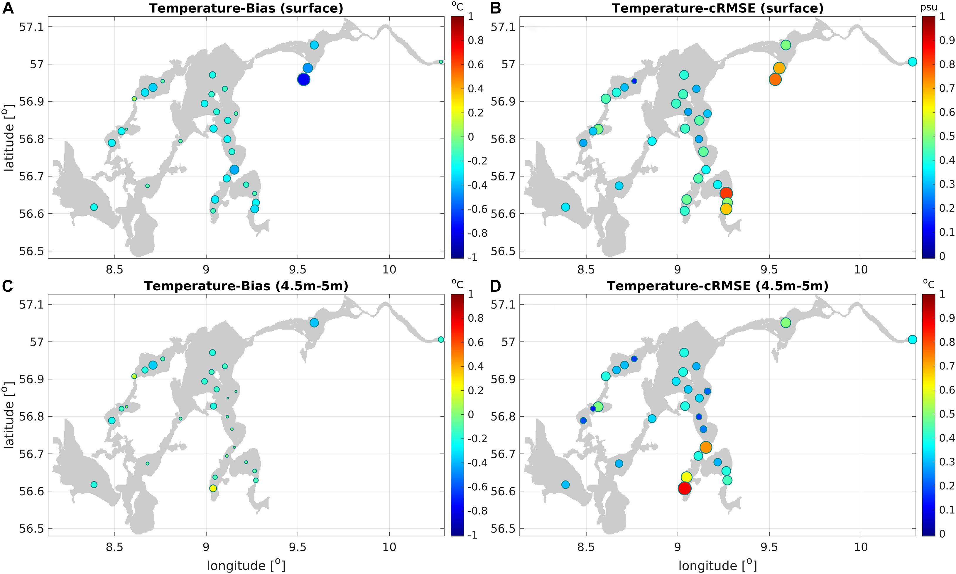
Figure 6. Bias (A,C) and cRMSE (B,D) of modeled water temperature at the surface (upper panel, A,B) and 4.5–5 m depth (lower panel, C,D) in the Limfjord. Each marker represents a station with at least 10 observations.

The model overestimates the upper layer salinity in the northern part of the Limfjord and underestimates salinity in Skive fjord, Lovns Bredning and Halkaer Bredning (near Sebbersund area), which are affected by major rivers (Figures 7A,C). The averaged cRMSE in the fjord is about 1 psu. At most stations, salinity cRMSE is less than 1 psu. Large cRMSE values are only found at stations in Lovns Bredning and Halkaer Bredning (Figures 7B,D).

FIGURE 7

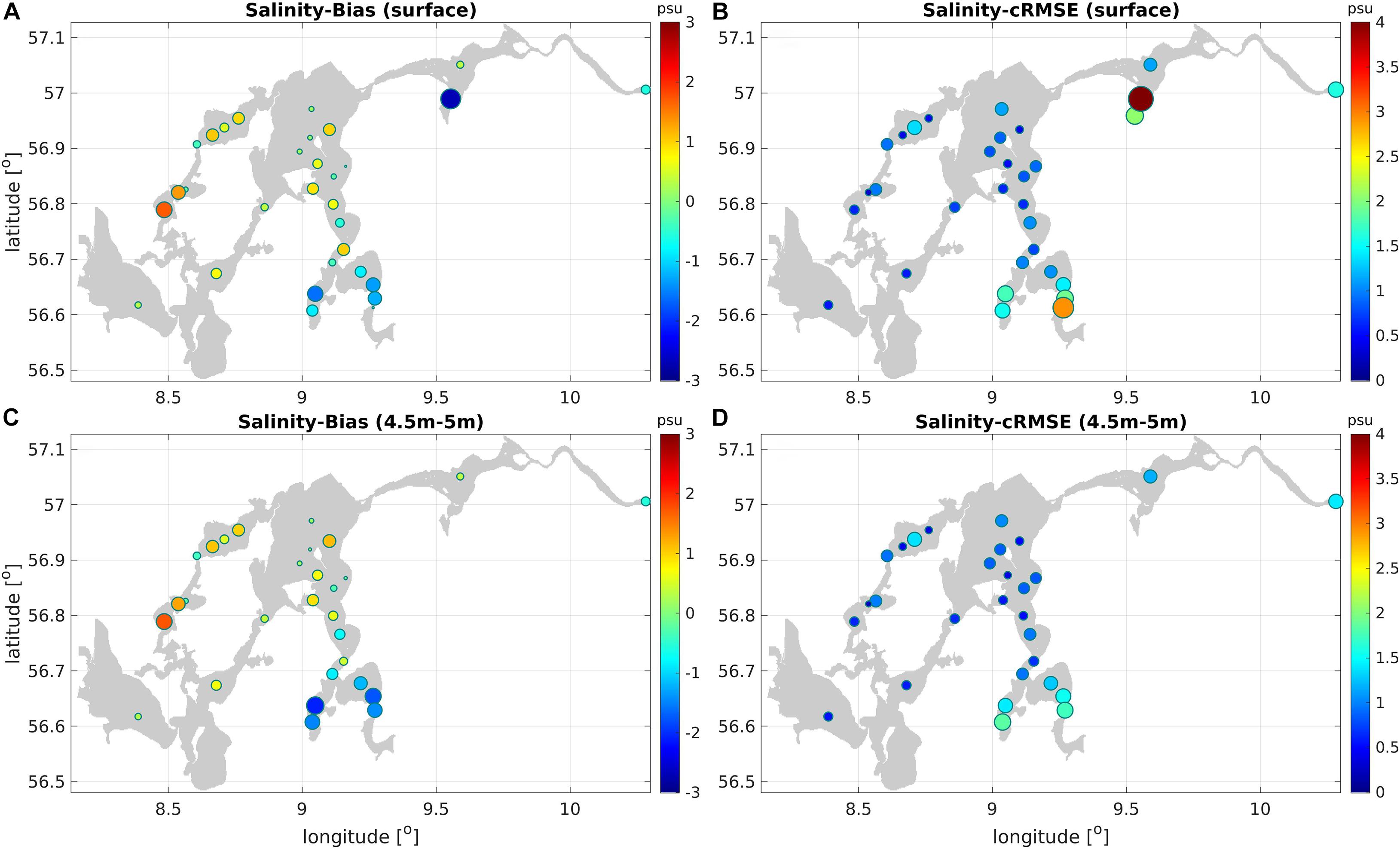
Figure 7. Bias (A,C) and cRMSE (B,D) of modeled water salinity at surface (upper panel, A,B) and 4.5–5 m depth (lower panel, C,D) in the Limfjord. Each marker represents a station with at least 10 observations.

Modeling Vertical Distribution of T/S and Stratification

The model temperature is colder than observations in the upper 5 m. The largest negative temperature bias is found at the surface (−0.2°C). Below 6 m, the model ocean is slightly warmer than the observations. The cRMSE is almost constant in the upper 8 m. Below 8 m depth, cRMSE increases with depth. The correlation coefficient between the model and observation data is about 0.7 in the surface and decreases with depth (Figure 8A).

FIGURE 8

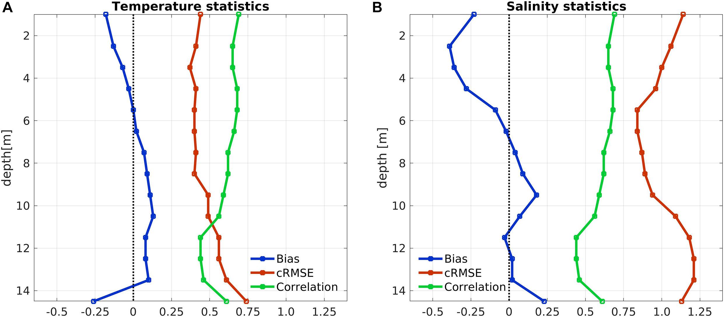
Figure 8. Vertical distribution of model error statistics: (A) water temperature and (B) salinity.

The vertical error distribution of salinity is similar to temperature. A negative salinity bias is characteristic for the upper 6 m (Figure 8B). At greater depths, between 6 and 10 m, the model water becomes saltier than observations. The cRMSE of salinity is larger at the surface (1.14 psu) and the bottom (1.21 psu), but decreases with depth at intermediate layers, to reach a minimum value of 0.84 psu at the depth of 6 m. The correlation coefficient between model and observed salinity is about 0.7 in the surface and decreases with depth (Figure 8A).

Although the Limfjord is very shallow, strong stratification is presented, most notably during summer period. The density stratification is mainly dominated by the presence of strong vertical salinity gradients. On average, deep layers are colder and saltier than the surface layer. Here we use surface-bottom difference of water temperature and salinity to represent the strength of the stratification. Simulated and observed stratification can be compared using a scatter plots (Figure 9). Considering the large variability of the stratification on synoptic and seasonal scales, the results with less than 20 observed profile samples were removed from the analysis in Figure 9, to reduce the bias due to sampling. The surface-bottom difference ranges from −1.5 to 0.5°C for water temperature (Figure 9A) and from 0 to 15 psu for salinity (Figure 9B). At one station near the eastern entrance of the Limfjord (10.31°E) the surface water is on average warmer than the bottom water. In general, the modeled, vertical temperature and salinity gradients agree with observations reasonably well. The correlation of the surface-bottom difference between the model and observed data is 0.97 for water temperature and 0.995 for salinity (Figure 9). However, it was also found that the modeled temperature stratification is too weak at most stations, which is indicated by the higher surface-to-bottom differences of the modeled temperatures in Figure 9A. The modeled temperatures are cooler than the observations at the surface but warmer at the bottom, which is probably related to too strong vertical mixing. Vertical profiles of mean salinity at individual stations indicate that the model is normally well mixed in the upper 2–3 m while observations often show a linear increase of salinity with depth (figures not shown).

FIGURE 9

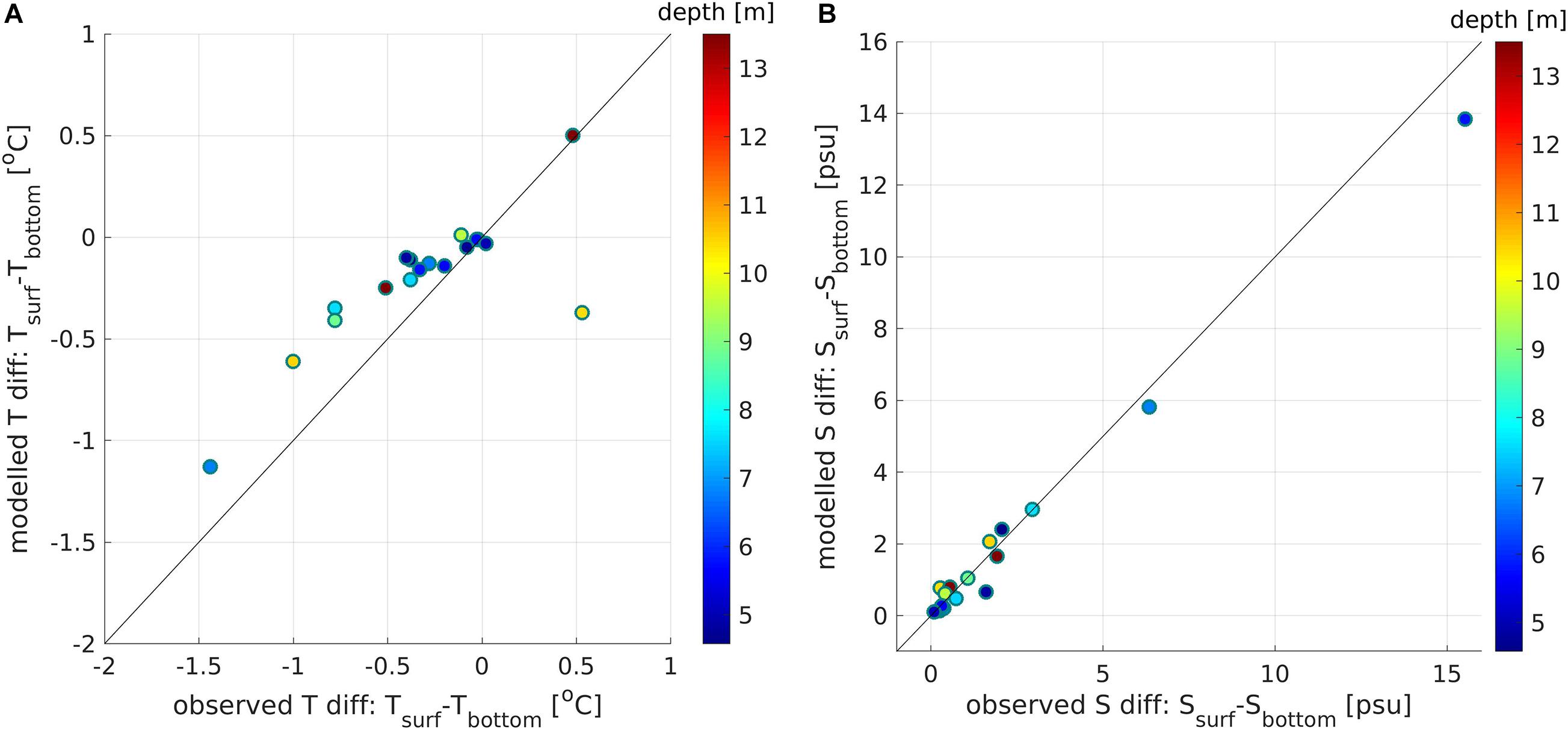
Figure 9. Scatter map of modeled and observed surface-bottom difference: (A) temperature; (B) salinity. Each marker represents a station with at least 20 observations.

Temporal Variability

Water temperature and salinity in the Limfjord has significant variability in diurnal, synoptic, seasonal and inter-annual scales. Observations obtained from research vessels are low in sampling frequency and can only resolve seasonal and inter-annual variability. Diurnal and synoptic variability of water temperature, for which an example is given in Figure 5, is usually not obtained. Results from Figure 5 indicate that the model is capable of resolving the variability on these time scales in reasonably good quality. On longer time scales, the model resolves the seasonal to inter-annual variability of salinity and temperature quite well. Inter-comparisons of the modeled and observed multi-year time series of water temperature and salinity at three stations are shown in Figure 10. The three stations at Oddsund, Nykøbing Mors, and Nibe Bredning represent the western, middle and eastern Limfjord, respectively. For temperature, both seasonal and inter-annual variability is well reproduced (Figures 10A,C,E). Especially at Nykøbing Mors, the maximum water temperatures in 2014, 2018, and 2019 are well simulated (Figure 10C). For salinity, at Oddesund station, there are several events e.g., in April 2018 and November 2019, when salinity drops significantly. These events are well simulated (Figure 10B). At station Nibe Bredning, observations show a stepwise reduction of salinity from December 2018 to February 2020, which is also successfully reproduced by the model (Figure 10F). At Nykøbing Mors, the relatively low salinity in summer 2016 and high salinity in summer 2019 are reproduced (Figure 10D).

FIGURE 10

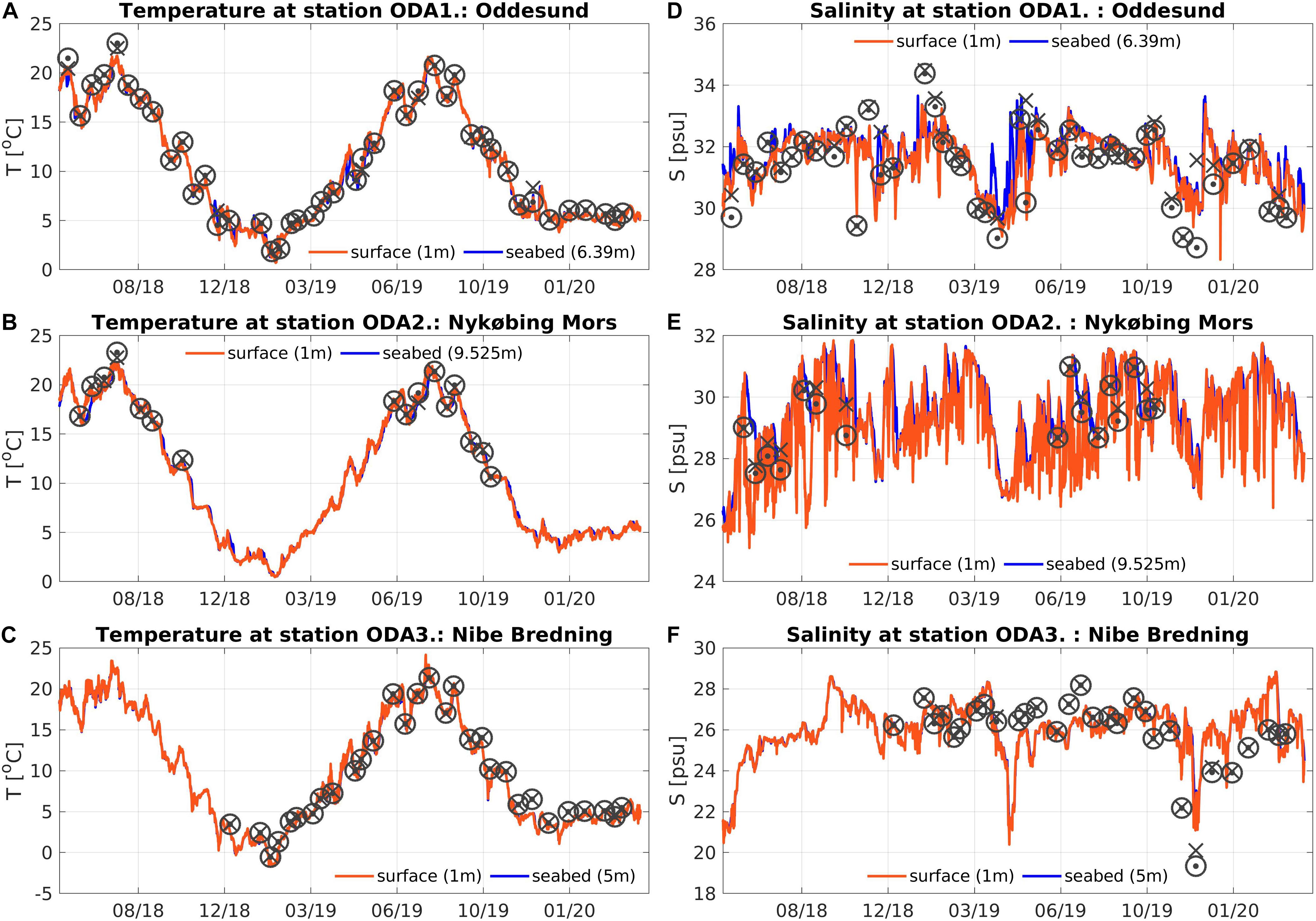
Figure 10. Time series of simulated and observed values of water temperature and salinity in the surface (A–C) and bottom (D–F) at station ODA1 (A,D), ODA2 (B,E), and ODA3 (C,F) in Figure 1. Observed values at the surface are shown as black circles with dots, whereas observed values near the sea bed are shown a crosses.

Model Applications for Mussel Fishery Management

Managing sustainable shellfish fishery in Danish coastal and fjord areas relies on tools and knowledge that combine in situ observations, modeling techniques and fishing activity. A recent Danish initiative, the TASSEEF project (Development of new tools to assess the environmental effects of fishing), investigated indirect effects of sediment plumes from fishing dredgers on the marine environment (Pastor et al., 2020). The project highlighted the benefit of hydrodynamic models for providing estimates of water currents at high spatial and temporal resolution. Participating models were validated against in situ observations for the prediction of sediment plume spreading. For the application in drift modeling of suspended sediment, the quality of the drift currents in a topographic complex area is essential. This is a challenging task for regional modeling with a relative coarse resolution.

Modeled and observed currents were compared at two locations in Lovns and Løgstør Bredning, respectively (Figure 1 shows the location of the two moorings). The observational data was collected during two monitoring campaigns in 2017 using moored ADCP instruments (Table 2 and Figure 11). At both locations, the currents were almost barotropic without significant vertical shear over most of the sampling period. At the Lovns mooring, currents were predominantly directed westward and southward. The strongest currents (up to 0.15 m s^–1) were measured during the first 2 days of sampling and weaker currents were recorded toward the end of the deployment. At Løgstør, currents were mainly directed to the northeast with velocities of up to 0.10 m s^–1, including short periods of flow reversal to southwestward flow.

FIGURE 11

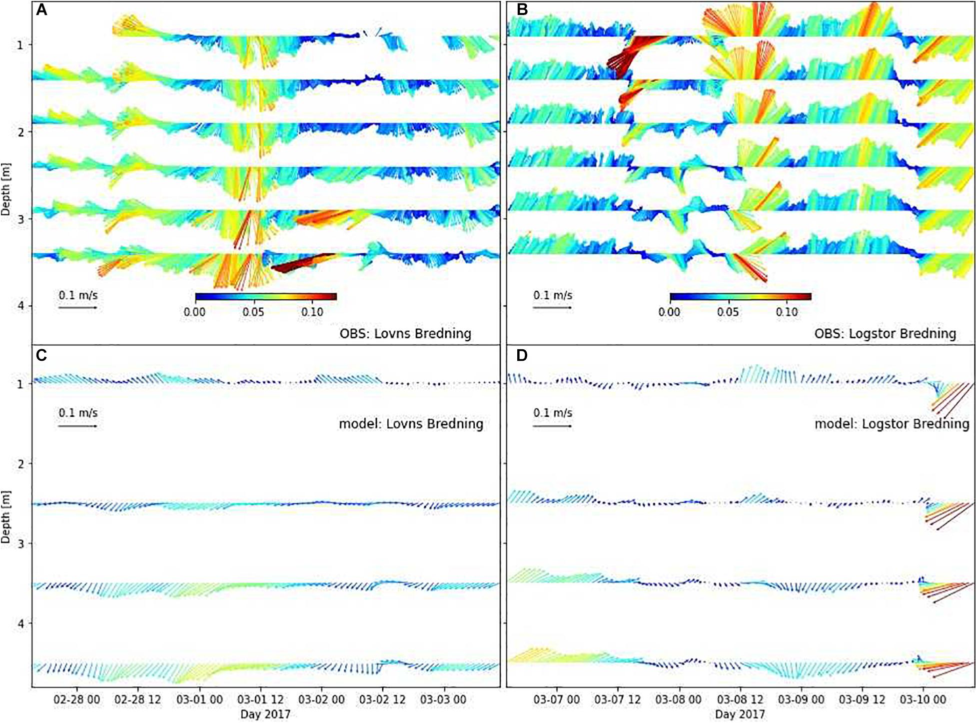
Figure 11. ADCP time series (top) of instantaneous currents (every 40th ensemble is shown corresponding to 10 min intervals) and simulated instantaneous current profiles (below) at Lovns Bredning (A,C) and Løgstør Bredning (B,D).

Hydrodynamic modeling of instantaneous ocean currents in the complex estuaries of the Limfjord is still challenging, because key processes like surface mixing needs to be adapted to the shallow, confined water body of the fjord. In the open oceans, wind dependent parameterizations following Craig and Banner (1994) are used to describe the injection of turbulent kinetic energy due to surface wave breaking. But inland water bodies like the Limfjord face weaker land-winds that do not always have the strength to drive surface mixing. For this reason, the shear and buoyancy production of turbulence was amplified at the surface, to produce realistic, vertical homogeneous current profiles like the ones that have been observed (Figure 11).

A direct way to qualitatively analyze the ocean currents is to visualize the zonal-and meridional components of the modeled and observed currents as time series (Figures 12, 13). Observed and modeled current pattern are quite variable, with frequently changing directions, which makes the presented cases an interesting study for fjord model development. The current patterns are strongly affected by the cross-basin water transport, which generates non-local currents that are not directly synchronized with the wind field. At Løgstøer for example, the wind turns from southwesterly, on February 7, 2017 (afternoon) to northeasterly direction, on February 9, 2017 (morning), undergoing a period of reversing directions (Figure 12). In theses 2 days, the measured currents make nearly two 180° turns, first against the wind, than turning back slowly into the wind. Løgstøer, in the central Limfjord, is stronger affected by the cross-basin water transport through the fjord. Lovns on the other hand, is situated in the southern branch of the fjord (Figure 13), and is more separated from the central part by the sound of Hvalpsund. Some of the non-local, cross-basin transport and related changes of the currents are filtered out by this narrow connection to the central Limfjord.

FIGURE 12

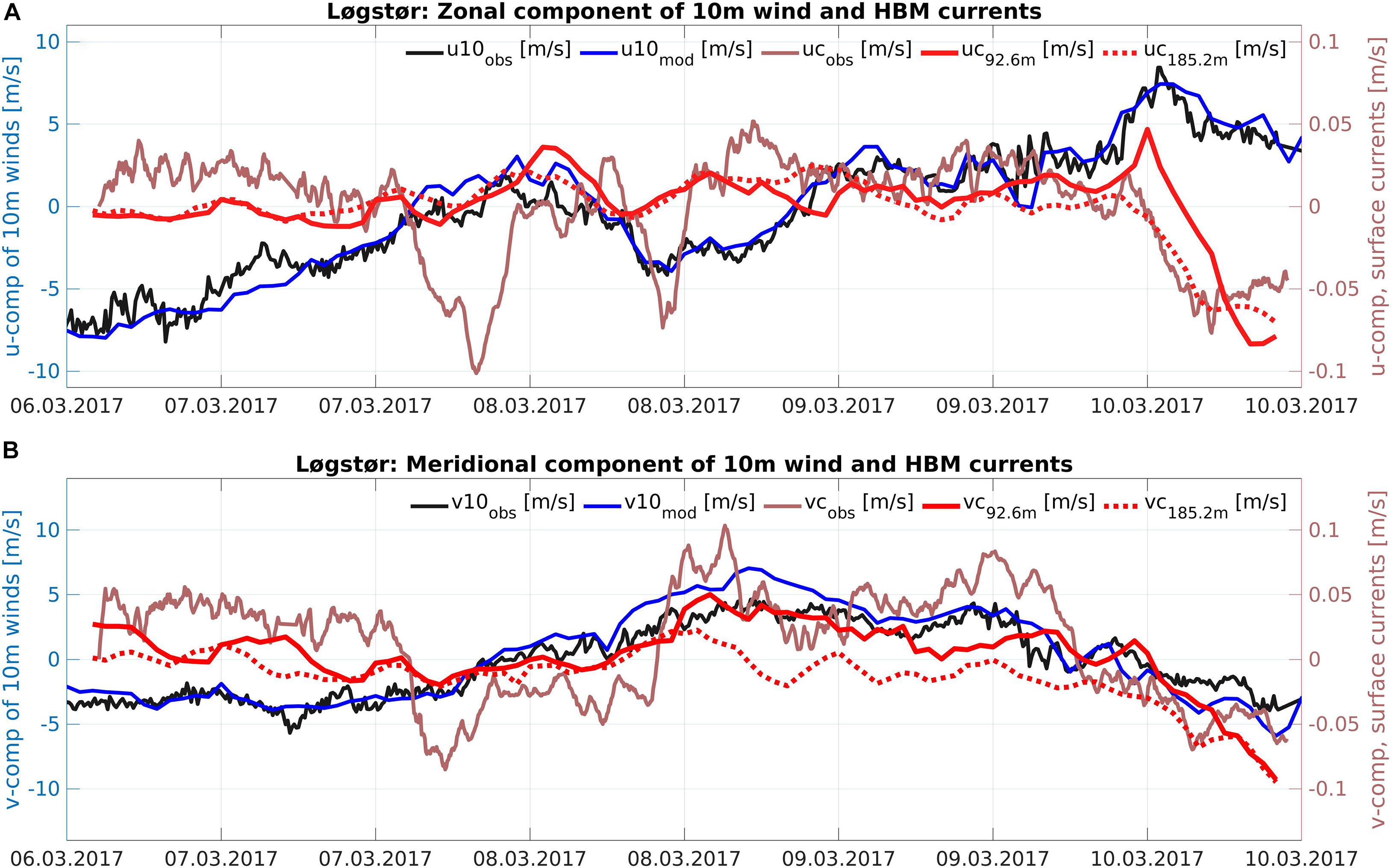
Figure 12. Logstør: Zonal (A) and Meridional (B) winds at 10 m height (u10, v10) and surface currents (uc, vc). Modeled winds (blue) and observed winds (black) at Aars Syd (56° 48′ 11.7″ N, 9° 31′ 3.9″ E) and modeled surface currents (bright red) and observed currents (faint red) at Løgstør. Full, red lines: double horizontal resolution (92.6 m), dotted red lines: standard resolution (185.2 m).

FIGURE 13

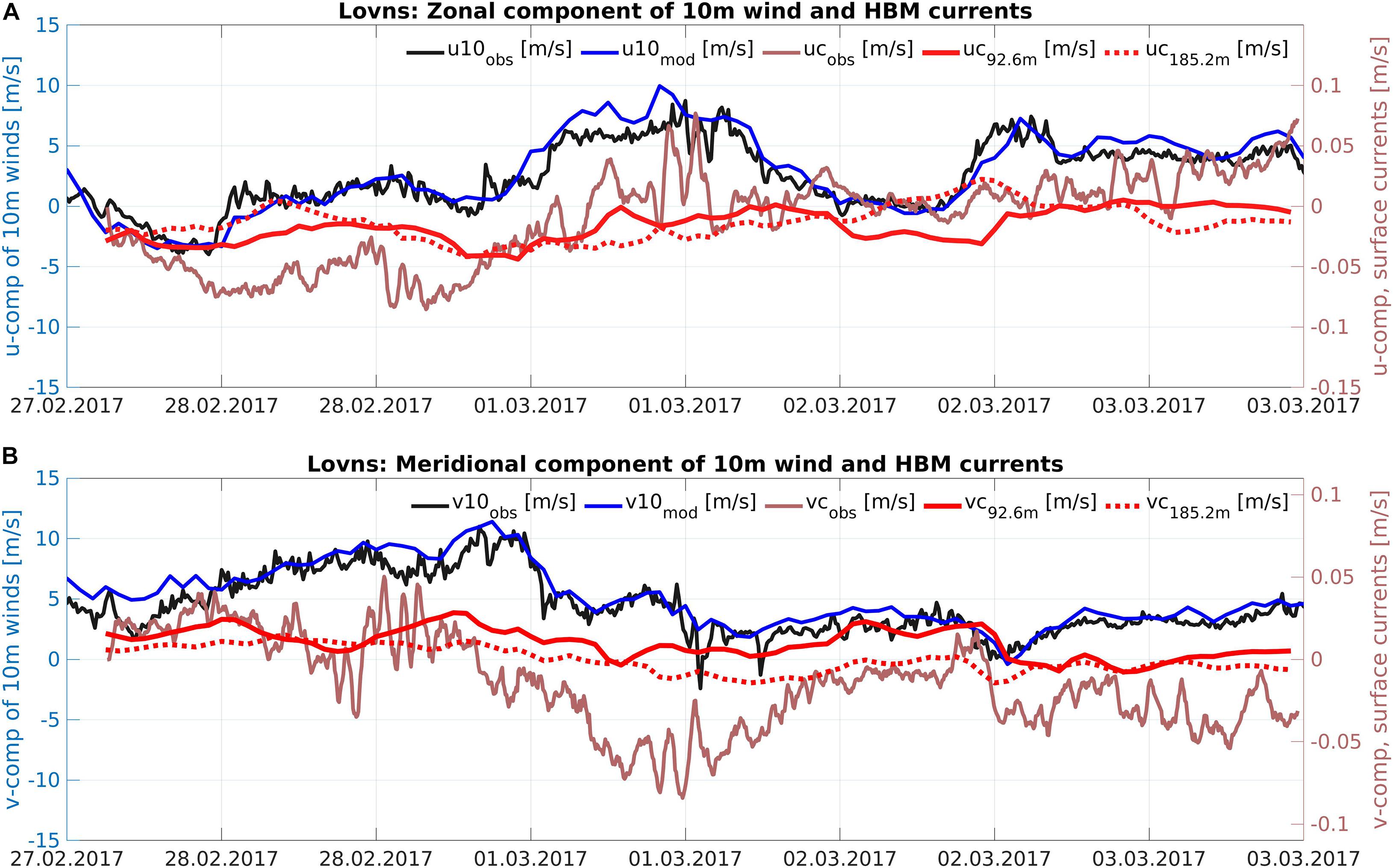
Figure 13. Lovns: Zonal (A) and Meridional (B) winds at 10 m height (u10, v10) and surface currents (uc, vc). Modeled winds (blue) and observed winds (black) at Aars Syd (56°48′11.7″N, 9°31′3.9″E) and modeled surface currents (bright red) and observed currents (faint red) at Lovns. Full, red lines: double horizontal spatial resolution (92.6 m), dotted lines: standard resolution (185.2 m).

The HBM model is performing reasonably well in situations of dominantly wind driven circulation but it is lagging behind when it comes to capture the faster changes in current speed, related to more “inertia like” movements. The limited transport capacity through the narrow sounds of the fjord plays a role in reducing the flow speed in the fjords interior, with consequences for the intra-basin exchange. This becomes apparent when the results of the original model simulation in 185.2 m horizontal resolution (Figures 12, 13 dotted lines) are compared with results of a simulation with double the resolution 92.6 m (Figures 12, 13, solid lines). This test was designed to study the effect of horizontal model resolution. Both set-ups share the same depth field, but not the same grid structure. The double resolution set-up was constructed by dividing each coarse grid cell into 2 × 2 horizontally neighboring fine grid cells. The high resolution run features a larger variability of the currents, but still does not reproduce the observed frequent directional changes in the period of reversing winds at Logstør. The spatial model resolution, however, is an important factor that can determine the strength and the direction of the currents (Figure 15). Progressive vector plots (PVP’s) illustrate this by following the path of a water parcel that flows with the currents at a given location. Forecasting errors accumulate along the pathways of the trajectories. Doubling the spatial model resolution reduces the cRMSE values for the component with the strongest errors (Figure 14) and gives a better vector representation of the model currents (Figure 15). The model error can be estimated as the distance between the observed and modeled endpoints of the trajectories, after 4 days of drift at sea. The doubling of the model resolution leads to a strong reduction of the forecasting error, from 7.04 to 2.31 km.

FIGURE 14

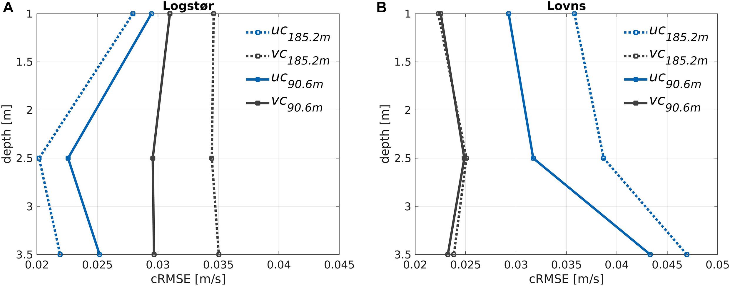
Figure 14. Centered RMS Error of zonal (blue) and meridional (black) currents at Logstør (A) and Lovns (B). Straight lines represent results of the run with standard horizontal resolution (185.2 m), whereas dotted lines represent the results of the run with double resolution (92.6 m).

FIGURE 15

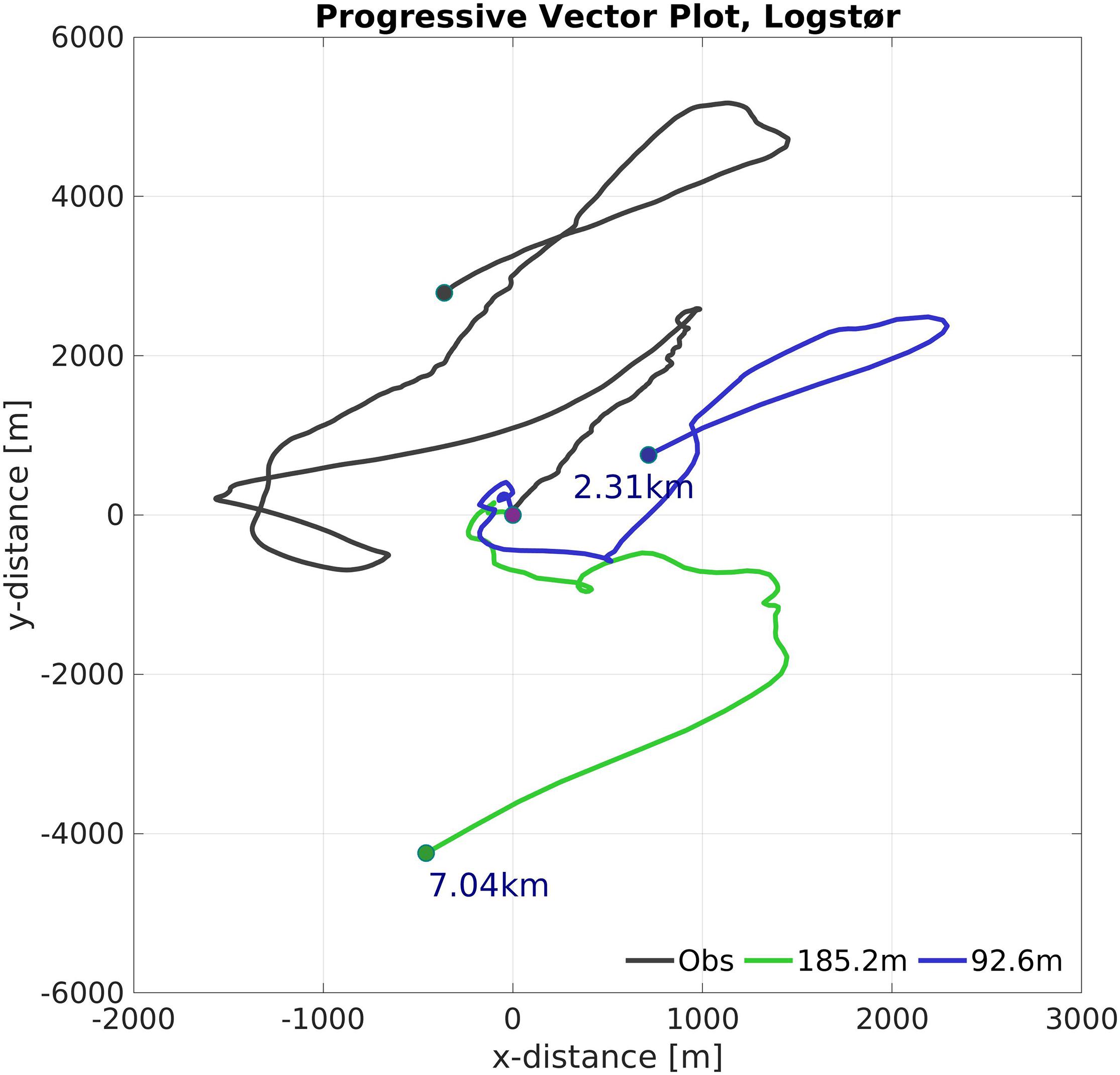
Figure 15. Progressive vector plot of surface currents at Løgstør: observed currents (black) and modeled currents with a grid resolution of 185.2 m (green) and 92.6 m (blue).

The model performance has been further evaluated using ADCP observations (Figure 11) at three model layers at 1 m/2.5 m/3.5 m (Figure 14), which roughly correspond to z-values of the observations of 0.91 m/2.41 m/3.41 m, with 3.41 m being the location of deepest observation. The total water depth is 5.5 m at Logstør and 4.6 m at Lovns. At both locations, the double resolution decreases the cRMSE at the surface for one component, from 3.46 to 3.1 cm/s for the v-component at Løgstøer and from 3.59 to 2.97 cm/s for the u-component at Lovns, but increases for the other component, from 2.79 to 2.95 cm/s for the u-component at Løgstør and negligibly, from 2.23 to 2.25 cm/s for the v-component at Lovns. The effect is more or less uniform over the entire water column. At Løgstør, the cRMSE values are largest near the surface, where the amplitude of the “inertia like” currents in the period of reversing wind and current directions is strongest. In the deeper layer, at distance of 1.59 m from the sea bed, the cRMSE values increase again, which is likely the consequence of the crude implementation of bottom friction, which uses a universal constant of 0.0015 for the open ocean and coastal, estuary waters alike.

The model current validation shows the quality of the HBM model in predicting ocean currents at the two very different geographical locations: at Løgstør, in the central, open Limfjord and at Lovns, situated in a side-estuary with complex bathymetry. The spatial resolution plays a decisive role in enhancing the flow through the narrows of the fjord, enhancing the capacity for intra-basin exchange, with positive consequences for the variability of the ocean currents at the two sites. Computationally efficient numerical models with the possibility to adapt the spatial and temporal resolution to the dynamic requirements in the narrows connections between the sub-basins are needed to build up an operational service for ocean currents and the transport of pollutants and other substances at sea.

Discussion and Conclusion

Enhancing monitoring and forecasting capacities of the marine environment in European and global coastal seas is an essential strategy to both support coastal management and to understand impacts of a changing ocean in a warmer climate (von Schuckmann et al., 2020). Coastal seas play a vital role as a key link between human activities, physical and biological processes, and marine ecosystem. This role is, however, often unquantified or under-represented in global and basin-scale ocean models (Holt and Proctor, 2008). CMEMS aims to narrow this gap with its large portfolio of ocean monitoring services and high-resolution modeling products for European seas, but currently available model services for Danish waters do not include the Limfjord. Our model showed an efficient two-way nested solution to provide accurate forecasts of storm surges, ocean currents, temperature and salinity as an important service to local communities and industries.

A comprehensive validation is given for assessing model performance in the entire Limfjorden for service applications. Sea level assessments focussed on model applications for operational storm surge prediction, by evaluating mean and peak error statistics for skill factor analysis. Comparing the fully nested model system for the North Sea, Baltic Sea and Limfjord with DMI’s operational, stand-alone storm surge model for the Limfjord, it was found that the nested system has the better overall performance, with lower cRMSE’s of 8.4 and 6.7 cm in the western and central Limfjord, respectively, in comparison with 10.4 and 8.2 cm of the stand-alone model, but that the stand-alone model has the better performance at targeted stations in the eastern Limfjord: 9.24 cm, compared with 9.3 cm of the fully nested system. The ability to tune boundary conditions makes the stand-alone model more adaptable to local conditions at given sites, here Aalborg, Denmark’s fourth biggest city and one of its largest shipping harbors. This advantage of the stand-alone model does not extend to peak errors, which are generally larger in the western, central and eastern fjord: 6.4, 6.9, and −5.2 cm, in comparison to the values of the nested setup: −0.8, 3.8, and 2.9 cm. Storm surge events are more difficult to tune than average situations, especially in the interior of the fjord. An over-prediction of the event is accepted, in order to avoid a missed warning. Fully nested set-ups provide a possibility to further develop the storm surge service and to reduce peak errors and miss rates.

The HBM stand-alone model has provided reliable operational storm surge predictions for the Limfjord since 2007. It has been continuously developed, to improve the model performance in coastal and estuary scales, leading to further reductions of the forecast errors for salinity and temperature predictions, in the project TASSEEF and the EU H2020 project FORCOAST, dedicated to develop model applications for aqua-farming. Horizontal and vertical distribution of simulated water temperature and salinity agreed well with observations in all major sub-basins of the Limfjord. Important parameters and processes including shallow water temperature and its variablity on diurnal to seasonal time scale is significantly improved by using a modified radiation attenuation formula. In addition, salinity stratification is also well reproduced by the model. The correlation coefficient between modeled and observed surface-bottom differences are 0.995 for salinity and 0.97 for temperature. Modeled water temperature has a negative bias of −0.2°C at the surface and 0.1°C at 4.5 m depth and a cRMSE of 0.42°C at the surface and 0.37°C at 4.5 m depth. For the salinity, the model has a negative bias of about −0.25 psu in the upper 4 m while cRMSE is 1.14 psu at the surface and 0.96 psu at the 4.5 m depth. There is still scope for improvement, especially in local bays with very narrow passages and high river discharge. Higher model resolution is needed to resolve land-fjord water exchange. In addition, variability on synoptic scales of the Limfjorden hydrographic state, such as saline inflow events from the west and brakish water intrusion from the east, stratifying and de-stratifying processes, was not extensively verified in this study due to lack of observations. North Sea-Baltic Sea water exchange through the fjord is mainly dominated by the zonal sea level gradient. Thus, episodic saline inflow events from the North Sea boundary can be well resolved considering a high quality sea level forecast by the model.

The North Sea-BalticSea water exchange through the fjord is largely determined by the transport through the narrow sounds of the Limfjord, whose capacity controls the flow pattern in the central parts of the Limfjord. The fishery management project TASSEEF studied this further by assessing the impacts of mussel dredging on sediment plume formation and drift pattern (Pastor et al., 2020). Two sites in the central part of the Limfjord were selected: Løgstør, along the main axis of the fjord and Lovns, in an estuary with complex bathymetry. It was found, that the spatial resolution of the model plays a decisive role in enhancing the flow through the fjord, with positive impacts on the variability and the cRMSE of the current components at the two sites. At Løgstør, the doubling of the model resolution, from 185.2 to 92.6 m horizontally, led to a reduction of about 10.4% of the cRMSE for the meridional component, from 3.42 to 3.1 cm/s at the surface, but also to an increase of the cRMSE value for the zonal component by 5.7%, from 2.79 to 2.95 cm/s. The flow pattern were largely improved, demonstrated by a large reduction of the distance between observed and modeled drift location in a progressive vector plot, from 7.04 to 2.37 km. At Lovns, in the southern Limfjord, separated from the central part by the sound of Hvalpsund, the model performance generally improves by the increase in resolution. The cRMSE of the zonal component decreases by 17.3%, from 3.59 to 2.97 cm/s, at the surface, while the cRMSE of the meridional component remained unchanged. It is likely that a further increase in spatial resolution of the model set-up will lead to further improvements of the model performance. This requires computationally efficient numerical models with the possibility to resolve the entire fjord and the narrow sounds in appropriate resolution.

Ocean circulation model have been continuously developed from basin scale hydrodynamic model to high-resolution coastal-estuary model for a wide range of applications, from storm surge warning, supporting aqua-farming to fishery management. The key driver for this has been the establishment of a value chain driven by end-user needs to support sustained development, and to deliver valuable services and products. For HBM, this development has been following two branches: (1) improving the model physics and adapting the relevant model processes, e.g., for short wave radiation in shallow waters, and surface turbulence production; and (2) by improving the numerical efficiency and dynamical two-way nesting routines of the model, to be able to run memory demanding seamless model applications that zoom in from the basin scales onto the coastal-estuary scales. This integrated system allows the continuous extension of the service, to cover regions that are currently not part of the CMEMS information system. It has proven to provide the best overall performance for sea level, salinity, temperature and current in the Limfjord domain, but it has also shown to be more resource demanding. A separate, stand-alone model could use higher resolution and still provide a faster service. This would be beneficial for resolving the water exchange between the sub-basins of the fjord and could improve transport and drift simulations. It could provide a good option for a targeted user with specific interest in selected sites, as the boundary conditions can be tuned to improve the model performance. But this advantage can’t be easily extended to other sites. Therefore it would only provide an option for a user interested in specific applications, oyster-farming in the western Limfjord, for example. The two approaches can be further developed, by employing local-area, stand-alone models from local providers to develop downstream services for interested users, and by further enhancing the CMEMS modeling capacity to coastal end estuary scales using nested models.

Data Availability Statement

The raw data supporting the conclusions of this article will be made available by the authors, without undue reservation.

Author Contributions

JM and JS designed the concept of the research. JN and JM developed and maintained the HBM operational set-up for the North Sea, Baltic Sea, and Limfjord. The HBM model has been developed by a group of people in the BalMFC consortium, including the authors. All authors contributed to data processing and data analysis: JM and JN to sea level assessments; JS and VF to the temperature and salinity model evaluation; CM and JM to hydrodynamic drift assessments. All authors contributed to the manuscript.

Funding

We are grateful to be supported by the EU-H2020 funded project FORCOAST (grant agreement ID 870465) and appreciate the support that we have received from the Danish Ministry of Food and Environment (EMFF) in the TASSEEF project (grant no. 33113-I-16-011). VF is grateful to be supported by the Latvian Fundamental and Applied Research Project lzp-2018/1-0162.

Conflict of Interest

The authors declare that the research was conducted in the absence of any commercial or financial relationships that could be construed as a potential conflict of interest.

Footnotes

1. ^ https://odaforalle.au.dk/ hosted by DCE.

References

Axell, L. B. (2002). Wind driven internal waves and Langmuir circulations in a numerical ocean model of the southern Baltic Sea. J. Geophys. Res. 107: 3204.

Google Scholar

BalMFC Group (2014). “MyOcean baltic sea monitoring and forecasting centre, conference: operational oceanography for sustainable blue growth: the seventh EuroGOOS conference, Lisbon” in Proceedings of the Seventh EuroGOOS Conference, eds E. Buch, Y. Antoniou, D. Eparkhina, and G. Nolan (Brussels: EuroGOOS), 33–42.

Google Scholar

Berg, P. (2012). Mixing in HBM. DMI Scientific Report No. 12-03. Copenhagen: Danish Meteorological Institute, 21.

Google Scholar

Berg, P., and Poulsen, J. W. (2012). Implementation Details for HBM. DMI Technical Report No. 12-11. Copenhagen: Danish Meteorological Institute, 149.

Google Scholar

Brüning, T. (2020). Improvements in turbulence model realizability for enhanced stability of ocean forecast and its importance for downstream components. Ocean Dyn. 70, 693–700. doi: 10.1007/s10236-020-01353-9

CrossRef Full Text | Google Scholar

Canuto, V. M., Howard, A. M., Cheng, Y., Muller, C. J., Leboissetier, A., and Jayne, S. R. (2010). Ocean turbulence, III: new GISS vertical mixing scheme. Ocean Model. 34, 70–91. doi: 10.1016/j.ocemod.2010.04.006

CrossRef Full Text | Google Scholar

Canuto, V. M., Howard, A., Cheng, Y., and Dubovikov, S. (2002). Ocean turbulence. Part II: vertical diffusivities of momentum, heat, salt, mass, and passive scalars. J. Phys. Oceanogr. 32, 240–264. doi: 10.1175/1520-0485(2002)032<0240:otpivd>2.0.co;2

CrossRef Full Text | Google Scholar

Christiansen, T., Christensen, T. J., Markager, S., and Jens Kjerulf Petersen, J. K. (2006). Limfjorden I 100 år – Klima, hydrografi, n ringsstoftilf rsel, bundfauna og fisk i Limfjorden fra 1897 til 2003. Technical Report No 578, Danish Centre for Environment and Energy DCE.

Google Scholar

Craig, P. D., and Banner, M. L., (1994). Modeling wave-enhanced turbulence in the ocean surface layer. J. Phys. Oceanogr. 24:2546. doi: 10.1175/1520-0485(1994)024<2546:MWETIT>2.0.CO;2

CrossRef Full Text | Google Scholar

Dick, S., Müller-Navarra, S. H., Klein, H., Komo, H., and Kleine, E. (2001). The Operational Circulation Model of BSH (BSHcmod) - Model Description and Validation. Technical Report, DE_ 2003:01411; DE. Hamburg: Bundesamt fuer Seeschiffahrt und Hydrographie, 53.

Google Scholar

Donnelly, C., Andersson, J. C. M., and Arheimer, B. (2016). Using flow signatures and catchment similarities to evaluate a multi-basin model (E-HYPE) across Europe. Hydr. Sci. J. 61, 255–273. doi: 10.1080/02626667.2015.1027710

CrossRef Full Text | Google Scholar

Fairall, C. W., Bradley, E. F., Hare, J. E., Grachev, A. A., and Edson, J. B. (2003). Bulk parameterisation of air-sea fluxes: updates and verification for the COARE Algorithm. Am. Meteorol. Soc. 16, 571–591. doi: 10.1175/1520-0442(2003)016<0571:BPOASF>2.0.CO;2

CrossRef Full Text | Google Scholar

Frandsen, R. P., Eigaard, O. R., Poulsen, L. K., Tørring, D., Stage, B., Lisbjerg, D., et al. (2015). Reducing the impact of blue mussel (Mytilus edulis) dredging on the ecosystem in shallow water soft bottom areas. Aquat. Conserv. 25, 162–173. doi: 10.1002/aqc.2455

CrossRef Full Text | Google Scholar

Hofmeister, R., Burchard, H., and Bolding, K. (2009). A three-dimensional model study on processes of stratification and de-stratification in the Limfjord. Cont. Shelf Res. 29, 1515–1524. doi: 10.1016/j.csr.2009.04.004

CrossRef Full Text | Google Scholar

Holmer, M., Ahrensberg, N., and Jørgensen, N. P. (2003). Impacts of mussel dredging on sediment phosphorus dynamics in a eutrophic Danish fjord. Chem. Ecol. 19, 343–361. doi: 10.1080/02757540310001596708

CrossRef Full Text | Google Scholar

Holt, J., and Proctor, R. (2008). The seasonal circulation and volume transport on the northwest European continental shelf: a fine-resolution model study. J. Geophys. Res. 113:C06021.

Google Scholar

Kara, B. A., Hulburt, E. H., and Wallcraft, A. J. (2005). Stability-dependent exchange coefficients for air-sea fluxes. J. Atmos. Oceanic Technol. 22, 1080–1094. doi: 10.1175/JTECH1747.1

CrossRef Full Text | Google Scholar

Knudsen, S. B., Ingvardsen, S. M., Madsen, H. T., Sorensen, C., and Christensen, B. B. (2012). Increased water levels due to morphodynamic changes: the Limfjord, Denmark. Coastal Eng. Proc. 1:49. doi: 10.9753/icce.v33.management.49

CrossRef Full Text | Google Scholar

Krause-Jensen, D., Greve, T. M., and Nielsen, K. (2005). Eelgrass as a bioindicator under the european water framework directive. Water Resour. Manage. 19, 63–75. doi: 10.1007/s11269-005-0293-0

CrossRef Full Text | Google Scholar

Larsen, J., Mohn, C., Pastor, A., and Maar, M. (2020). A versatile marine modelling tool applied to arctic, temperate and tropical waters. PLoS One 15:e0231193. doi: 10.1371/journal.pone.0231193

PubMed Abstract | CrossRef Full Text | Google Scholar

Maar, M., Timmermann, K., Petersen, J. K., Gustafsson, K. E., and Storm, L. M. (2010). A model study of the regulation of blue mussels by nutrient loadings and water column stability in a shallow estuary, the Limfjorden. J. Sea Res. 64, 322–333. doi: 10.1016/j.seares.2010.04.007

CrossRef Full Text | Google Scholar

Meier, M. H. E. (2001). On the parameterization of mixing in three-dimensional Baltic Sea models. J. Geophys. Res. 106, 30997–31016. doi: 10.1029/2000jc000631

CrossRef Full Text | Google Scholar

Pastor, A., Larsen, J., Hansen, F. T., Simon, A., Bierne, N., and Maar, M. (2021). Agent-based modeling and genetics reveal the Limfjorden as a well-connected system for mussel larvae. Mar. Ecol. Prog. Ser. DYNMODav2, 1–13. doi: 10.3354/meps13559

CrossRef Full Text | Google Scholar

Pastor, A., Larsen, J., Mohn, C., Saurel, C., Petersen, J. K., and Maar, M. (2020). Sediment transport model quantifies plume length and light conditions from mussel dredging. Front. Mar. Sci. 7:576530. doi: 10.3389/fmars.2020.576530

CrossRef Full Text | Google Scholar

Poulsen, J. W., and Berg, P. (2012). ). More Details HBM – General Modelling Theory and Survey of Recent Studies. DMI Technical report No. 12-16. Copenhagen: DMI.

Google Scholar

Poulsen, J. W., Berg, P., and Raman, K. (2015). “Better Concurrency and SIMD on HBM,” in High Performance Parallelism Pearls - Multicore and Many-core Programming Approaches, eds J. Jeffers and J. Reinders (Burlington, MA: Morgan Kaufmann).

Google Scholar

She, J., and Murawski, J. (2018). “Towards seamless modelling for the Baltic Sea. in operational oceanography serving sustainable marine development,” in Proceedings of the Eight EuroGOOS International Conference. 3-5 October 2017, Bergen, eds E. Buch, V. Fernández, D. Eparkhina, P. Gorringe, and G. Nolan (Brussels: EuroGOOS), 233-241.

Google Scholar

Smagorinsky, J. (1963). General circulation experiments with the primitive equations. Mon. Weather Rev. 91, 99–164. doi: 10.1175/1520-0493(1963)091<0099:GCEWTP>2.3.CO;2

CrossRef Full Text | Google Scholar

Thodsen, H., Eugenio, M. N., Nielsen, J. W., Larsen, J., and Maar, M. (2018). Afstrømning og Næringsstoftilførsler til Limfjorden Baseret på tre Forskellige Modeller (Teknisk rapport fra DCE - Nationalt Center for Miljø og Energi; No. 115). Aarhus: Aarhus Universitet, 20.

Google Scholar

von Schuckmann, K., Le Traon, P.-Y., Smith, N., Pascual, A. S., Djavidnia, S., Gattuso, J.-P., et al. (2020). Copernicus marine service ocean state report, issue 4. J. Operat. Oceanogr. 13(Suppl.1), S1–S172. doi: 10.1080/1755876X.2020.1785097

CrossRef Full Text | Google Scholar

WFD-EU. (2009). WFD CIS Guidance Document No. 20. Common Implementation Strategy for the Water Framework Directive (2000/60/EC). Luxembourg: European Communities, 46.

Google Scholar

Wiles, P. J., van Duren, L. A., Häse, C., Larsen, J., and Simpson, J. H. (2006). Stratification and mixing in the Limfjorden in relation to mussel culture. J. Mar. Syst. 60, 129–143. doi: 10.1016/j.jmarsys.2005.09.009

CrossRef Full Text | Google Scholar