Behavioral Response Study on Seismic Airgun and Vessel Exposures in Narwhals

Introduction

Anthropogenic activities such as shipping, seismic exploration, pile driving, dredging, ice breaking, and sonar and military activities introduce underwater noise pollution in both coastal and open ocean areas (Hildebrand, 2009). The noise pollution has, in some areas, been raised to levels where it can be considered a threat to marine life and especially to marine mammals that rely heavily on sound for orientation and communication (Richardson et al., 1995; Southall et al., 2007; Moore et al., 2012a; Reeves et al., 2014; Simmonds et al., 2014; Williams et al., 2015; Graham et al., 2019). Several studies of the effects of noise on marine mammals have documented a broad range of negative effects, from masking of signals and avoidance behavior, to loss of hearing sensitivity, physical injury, cessation of feeding, and increased stress (Richardson et al., 1995; Hildebrand, 2005; Weilgart, 2007; Rolland et al., 2012; DeRuiter et al., 2013; Dunlop et al., 2018; Bröker, 2019).

Sonar activity, shipping, and seismic surveys are of special concern in terms of ocean noise pollution and impacts on marine mammals (Weilgart, 2007; Bernaldo de Quirós et al., 2019; Elliott et al., 2019). While shipping and seismic surveys both produce low-frequency sounds that can travel long distances in the ocean, high-amplitude airgun pulses, used in seismic surveys for exploring the seabed, are of particular concern because these pulses can be detected over long distances and may result in disturbance effects far from the sound source (Hildebrand, 2009).

The North Atlantic is frequently affected by wide-ranging seismic surveys (Nieukirk et al., 2012), some of which can be detected in high Arctic areas where anthropogenic noise is rarely encountered (Moore et al., 2012b; Ahonen et al., 2017). Even in high Arctic areas, local seismic surveys are periodically a concern for endemic marine mammal populations (Heide-Jørgensen et al., 2012; Martin et al., 2017; Kyhn et al., 2019). These surveys are conducted during the ice-free season when Arctic whales are either in coastal areas or migrating between summer and winter grounds. For marine mammals, the implications of seismic disturbances include physiological and behavioral responses that may result in raised energetic costs, reduced feeding attempts, extreme physiological activity, displacement from habitats and migration routes, and loss of communication with conspecifics (National Academies, 2017).

Quantification of these behavioral and physiological responses to human activities is challenging for deep-diving marine mammals that inhabit remote Arctic areas. An initial approach is to observe the short-term effects of disturbances in a controlled-dose experiment where the animals are exposed to a restricted amount of seismic activity over a few days (Dunlop et al., 2017, 2018). Even though this approach does not offer complete understanding of the long-term cumulative effects of continuous seismic disturbance, as would be the case under an industrial scenario, controlled exposure experiments, albeit limited in scope, can nevertheless inform about the probability and type of behavioral/physiological responses. These can inform environmental impact assessment of industrial activities.

The recent interest for oil exploration in both East and West Greenland has stressed the importance of conducting studies that assess the environmental impacts of disturbance to marine life in Greenland (Boertmann et al., 2020). Of special concern are the effects of seismic exploration. Even though all marine mammals can be considered vulnerable to sounds from airgun pulses (NRC, 2005), some are considered particularly susceptible to several types of disturbances, and the narwhal, Monodon monoceros, is one of those species (Richardson et al., 1995). Studies of short-term reactions to ship noise and ice breaking showed that narwhals reacted to low sound exposures of icebreaker noise of 105 dB re 1 μPa by leaving the area and not returning until the next day (Finley et al., 1990). There are no studies of the effects of airgun pulses and their longer-term effects on narwhal populations (Heide-Jørgensen et al., 2012).

Narwhals are distributed in the Atlantic sector of the high Arctic where about 80% of the world population is found in Baffin Bay-Davis Strait. Outside this area, only East Greenland and areas north of Svalbard have predictable concentrations of narwhals (Hobbs et al., 2019). The coastal summer grounds of narwhals are covered by fast ice during winter, but during summer, the whales exhibit a remarkable site fidelity and return on the same approximate dates to the preferred localities inside the summer grounds (Heide-Jørgensen et al., 2015). This extreme philopatry leaves narwhals vulnerable to anthropogenic disturbances that occur during summer or during their migrations to and from summer grounds.

In this study, we conducted an experiment involving airgun pulses and narwhals in a large, yet restricted fjord system in East Greenland over two seasons. The experiment hinged on tagging whales with acoustic and satellite tags and then subjecting these whales to airgun pulses at different distances in a set of trials. Received levels at the whales were estimated by relying on sound source verification (SSV) recordings obtained in the same environment. In a few cases, tag data could be used to confirm received levels of sound at the whales. The advantage of conducting the study in a fjord system is that the whales have strong site fidelity to the fjord and remain in the area during the summer. In contrast to an open-ocean situation, this makes them available for the duration of the experiment. Meanwhile, the fjord system is complex, with many side-fjords and large islands where the whales can periodically be left undisturbed. This also allows for new exposure situations when the vessel has circumnavigated the islands. The disadvantage with a fjord system is the side reflections of the airgun pulses generated from the steep mountains beneath the water surface. They cause reverberations of each shot, making it difficult to distinguish between primary and reflected pulses.

Prior to any exposure experiments, it is important to have a baseline of knowledge on the behavioral and physiological performance of the animal in its undisturbed environment. To that effect, we have been following this population of whales for seven seasons before the exposure study (Heide-Jørgensen et al., 2014, 2015, 2020; Garde et al., 2015; Watt et al., 2015; Williams et al., 2017; Blackwell et al., 2018; Ngô et al., 2019, 2021; Søltoft-Jensen et al., 2020; Tervo et al., 2021). The advantage of an extensive baseline study is also that methods of instrumentation and data collection, which are needed to assess the response of the whales, can be developed and properly tested before the exposure study.

The response of an animal to disturbance can be multifaceted; as it is not possible to cover all potential behavioral and physiological effects, decisions must be made on the practicality of sampling a few selected parameters. In this study, we attempt to integrate physiological information (heart rate), acoustic behavior, dive and locomotion activity, as well as displacement. This paper provides an overview of the experiment and presents information on the initial displacement response of the whales. Together with forthcoming studies, the study presented here contributes important information on changes in behavioral and physiological parameters in relation to the level of exposure and distance to anthropogenic disturbances. By integrating the effects of the above-mentioned parameters, the study may provide insights about the energetic costs of disturbance allowing for assessment of the resiliency of individuals to anthropogenic disturbances. The long-term effects of disturbances can be extended to the population scale and may contribute to the development of appropriate mitigation measures.

Materials and Methods

Study Area

The Scoresby Sound fjord system (hereafter Scoresby Sound) in East Greenland is the summer residence for an isolated population of narwhals (Figure 1). The fjord system is about 350 km long with many side branches of smaller fjords around one large island: Milne Land. The detailed bathymetry of the fjord system is not well known, but most of the inner parts of the fjords have depths that range to 1,000 m or deeper (Ryder, 1895; Digby, 1953). Extensive shallow areas are found in the northeastern part along Jameson Land. There are 12 active glaciers that feed ice and meltwater into the fjord system; this is supplemented by an inflow from the cold East Greenland current in the northern part of the entrance to the fjord system (Digby op. cit.). The main current out of Scoresby Sound is in the southern part of the entrance. Sea ice forms in October in the inner parts of the fjord system and by December, the entire fjord is ice covered. The sea ice persists through June; however, an open water polynya is present throughout the winter at the opening of Scoresby Sound (Digby op. cit.).

FIGURE 1

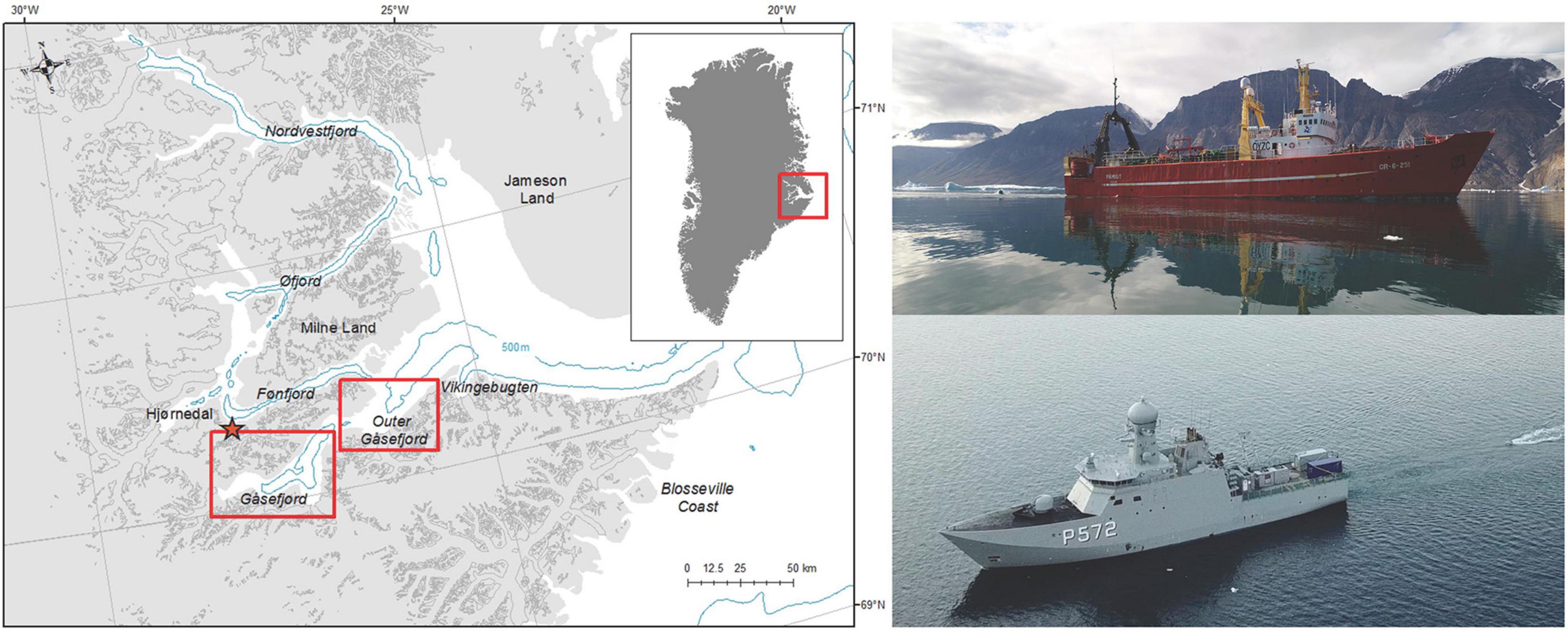
Figure 1. Map of study area in Scoresby Sound (left) with locality names and red boxes indicating trial areas shown in Figures 3, 4; the inset shows the location of the study area in East Greenland. The blue line is the 500-m isodepth. The upper right panel shows r/v Paamiut, and the lower right panel shows HDMS Lauge Koch, both while towing their respective airgun systems.

Study Design

Live Capture and Tagging of Narwhals

Live capture of narwhals was carried out from a field station at Hjørnedal in Scoresby Sound in collaboration with local Inuit hunters (Figure 1, see Heide-Jørgensen et al., 2015 for details). Set nets of either 40 or 80 m length and 5–8 m depth were deployed from shore to an anchor at suitable sites. Lookouts for whales were maintained from land-based promontories, from which the nets were kept under constant surveillance. When whales were observed in the area, several 6–8-m fiberglass boats were launched. As soon as the net buoys showed signs of a whale being entangled, the net was released from the anchor, and the whale was pulled to the surface and towards the shore. Instrumentation of captured whales lasted on average 13 min (SD, 2 min) and was conducted near the shore by four to six persons in survival suits standing next to the whale while supporting it. Total time in the net, from capture to release, was on average 50 min (SD, 22 min). Length of the whales and of the tusk, if present, was measured to the nearest centimeters, and sex of the whales was determined based on presence (male) or absence (female) of a tusk. Positioning of investigators on either side of the narwhal maintained the animal’s orientation during measurements and instrumentation. Overall behavior, respiration rate, and, in some cases, heart rate were monitored during and after the tagging process. Several types of instruments were deployed on the whales: two types of bolt-on satellite transmitters (Andrews et al., 2019), acoustic orientation tags, and heart rate recorders (Table 1). The types of tags used in the study are described below. Note that physiological monitoring of heart rate, respiration rate, and stroking acceleration in relation to dive depth was recorded using an ECG-ACC tag (UFI, Morro Bay, CA, United States, described in Williams et al., 2017) for a subset of the narwhals.

TABLE 1

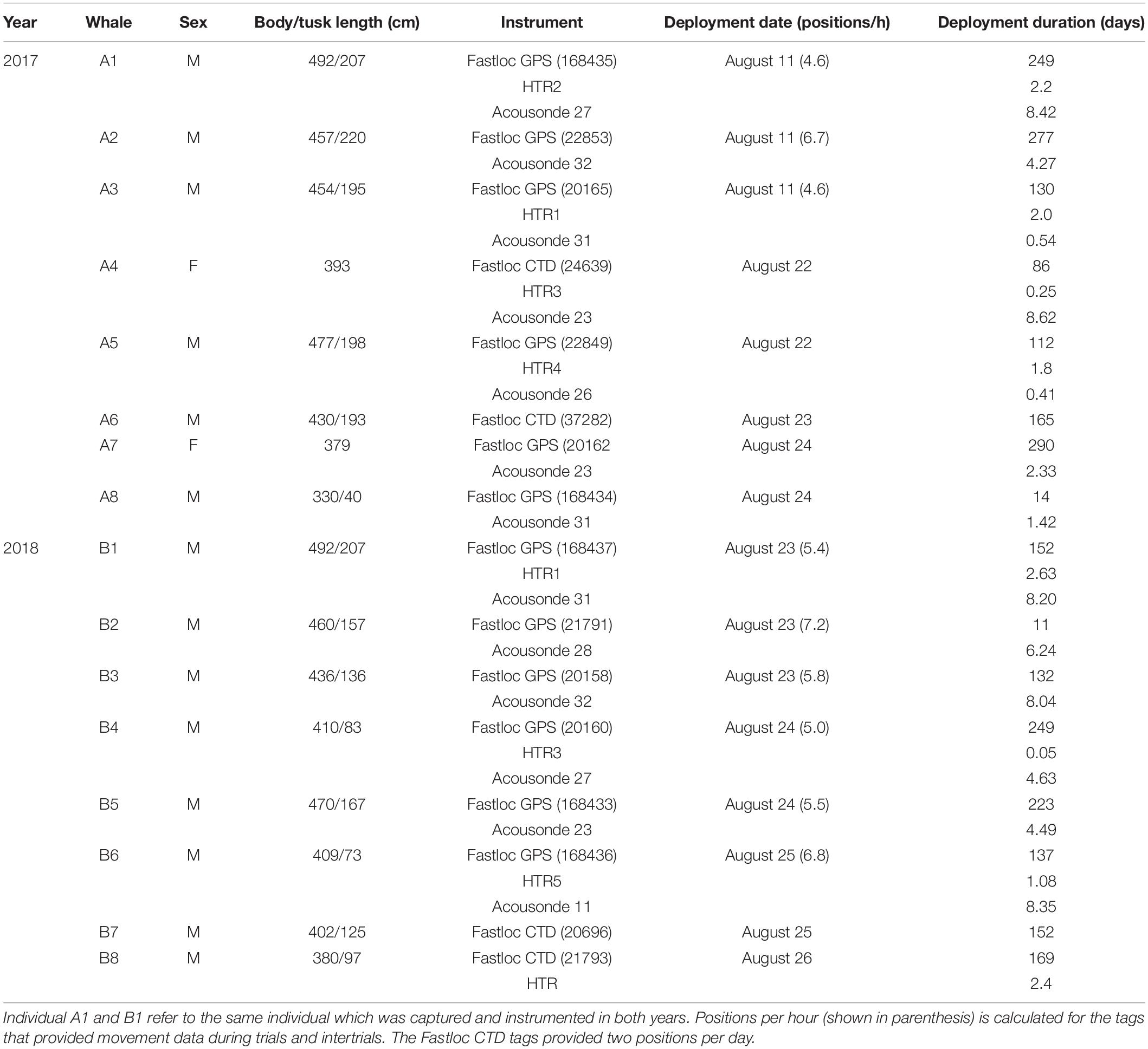
Table 1. Overview of instrumentations of narwhals in August 2017 and 2018 with Fastloc GPS receiver, Fastloc CTD tag, acoustic and orientation tags (Acousonde), and heart-rate recorders (HTR).

Fastloc GPS Receivers

Wildlife Computers (Redmond, WA, United States) Fastloc GPS receivers were mounted on the back of the whales with three 8-mm Delrin nylon pins secured with washers and bolts on each end, following instrumentation techniques used in similar studies in Canada and West Greenland (Heide-Jørgensen et al., 2003; Dietz et al., 2008). The transmitters were programmed to collect an unrestricted number of Fastloc snapshots through August. The Fastloc snapshots were transmitted to and relayed through the Argos Location and Data Collection System (argos-system.cls.fr). Post-processing of GPS positions was conducted through the Wildlife Computers web portal. Fastloc GPS is a positioning system with the ability of faster acquisition of animal positions than traditional GPS (Bryant, 2007; Tomkiewicz et al., 2010) with an accuracy of tens to hundreds of meters (Thomson et al., 2017).

In each of the two study years, two additional narwhals were instrumented with Fastloc CTD satellite transmitters that, in addition to depth, also recorded and transmitted data through the Argos Location and Data Collection System from two daily depth profiles of water temperature and salinity that were sampled at 1 Hz (Wildlife Computers Scout-CTD-370D, see Heide-Jørgensen et al., 2020; Teilmann et al., 2020). These tags were mounted in a similar way as the Fastloc transmitters, and each cast had an associated Fastloc position, resulting in only two positions per day from these tags.

Acoustic and Orientation Tag

Twelve whales were fitted with Acousonde^TM acoustic and orientation recorders¹, whose floats had been modified to accommodate an Argos transmitter (Wildlife Computers SPOT5) in addition to a VHF transmitter (ATS Telemetry, ATS, Isanti, MN, United States), to enable relocation of the tag after release from the whale. The Acousonde tags were mounted on the rear half of the animal along the side of the dorsal ridge. They were attached to the skin with suction cups, but in order to extend the longevity of the attachment, two 1-mm nylon lines were threaded through the top of the dorsal ridge, and the Acousonde was connected to the lines with magnesium corrosive links, which aimed to increase the attachment duration for up to 8 days after attachment.

Blackwell et al. (2018) developed a protocol for reliable detection of narwhal acoustic signals using a relatively low sampling rate. Hence, in order to extend record lengths, all deployments used continuous sampling at 25,811 Hz (16-bit resolution). The low frequency channel of the Acousonde includes an HTI-96-MIN hydrophone with a nominal sensitivity of −201 dB re 1 V/μPa, a preamp gain of 14 dB, an anti-aliasing filter (3-dB reduction at 9.2 kHz and 22-dB reduction at 11.1 kHz), and a high-pass filter with a 3-dB cutoff at 22 Hz. In addition, a 3D accelerometer was sampled at 100 Hz and a pressure transducer at 10 Hz.

Seismic Operation

In 2017, the seismic program was conducted from a research vessel r/v Paamiut (1084 GRT) during August 14–22. The vessel towed a GI gun type 210 (210 in.³ or 3.4 L) at a depth of 3 m and a speed of 5 knots. The airgun was operated at 115–120 bar (1,668–1,740 psi). At full volume (210 in.³), the estimated source level of this gun was ∼231 dB re 1 μPa at 1 m (peak-to-peak). It was set to fire every 12 s, and a GPS navigation system recorded the location of every shot. Paamiut used two standard echo sounders (Furuno 50 and 38 kHz), which were on continuously.

In 2018, the seismic program was operated from an offshore patrol vessel HDMS Lauge Koch between August 25 and September 1. The ship towed a cluster of two Sercel G-guns (total volume, 1,040 in.³ or 17.0 L) at 6 m depth and at a speed of 4.5 knots. The airgun cluster was operated at a mean pressure of 125 bar (1,813 psi; range, 115–135 bar). At full volume (1,040 in.³), the source level of the cluster was 241 dB re 1 μPa at 1 m (peak-to-peak, as simulated by the gun manufacturer). The guns in the cluster were fired synchronously every 80 s, and similarly to 2017, the GPS navigation system recorded the location of every shot. In addition, the Lauge Koch used a Reson Seabat 7160 multibeam echo sounder (hereafter, MBES; nominal operating frequency, 41–47 kHz), which was on continuously for mapping of the seafloor. The guns that were used in both 2017 and 2018 were at the lower range of sizes used by the typical industrial seismic operation with multigun arrays but were chosen, as they are capable of producing signals similar to larger airgun arrays.

In both years, real-time positions of the tagged whales were acquired within hours, and ship routes were adjusted to focus airgun pulse exposure to areas with whales. Shorter periods were assigned to expose the whales to a ship without an operating airgun. Firing of airguns was initiated before the ship arrived at the area with whales, and the maximum duration of exposure to airgun pulses was restricted to 5 h. Exposure time was, however, difficult to assess in the field because of the simultaneous movements of the whales and vessel, the speed of the vessel, the delay in acquiring whale positions, and the topography of the study area.

SoundTrap autonomous recorders (model ST300, Ocean Instruments, Auckland, New Zealand) were used in 2018 to collect SSV data for the two airgun sizes, as well as to verify the presence and received levels of sounds from the MBES. SoundTraps have a flat frequency response from 20 Hz to 60 kHz, internal storage of 256 GB, and were sampled continuously at a 96-kHz sampling rate. SoundTraps (up to three per SSV, to provide redundancy) were attached to one or two weighted lines hanging under a float, at a depth of 10 m. The float included a satellite tag (Fastloc GPS transmitter), which enabled range determination from the airguns throughout the SSVs and facilitated retrieving the recorders. SoundTraps were deployed off the side or stern of the Lauge Koch while in transit or from a launched smaller craft. Four SSVs (one with the 2017 smaller airgun and three with the 2018 larger airgun) were performed in areas where whales were subjected to airgun pulses (Table 2). The data from these four SSVs were used to describe received levels of sound as a function of distance.

TABLE 2

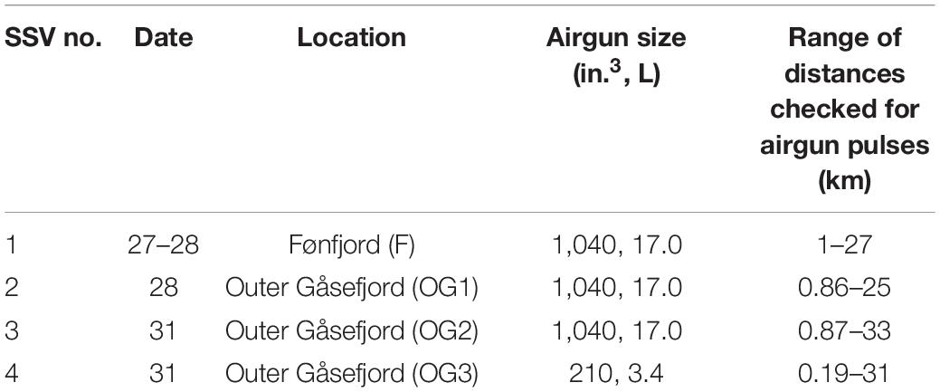
Table 2. Information pertaining to the sound source verifications (SSVs) performed in Scoresby Sound, East Greenland, in August 2018.

Data Analysis

Exposure of Narwhals to Airgun and Ship Noise

Individual whales were assumed to be exposed to seismic operation or ship noise during periods when the whale and the seismic operation vessel were in line of sight. Line of sight was determined post-hoc, based on maps of geographical positions of the ships and whales aligned in time (maps drawn with coastline of Scoresby Sound from Jepsen et al., 2005). There is no simple way to quantify the exposure when the whales were not in line of sight with the vessel because of the complex coastline, leading to situations in which the whales were behind a peninsula, promontory, or one of several rocky islands, such as the 4,000 km² Milne Land. Exposure was therefore only considered if whales were within line of sight of the vessel. When in line of sight, trials were defined as periods when the airgun was being used, while intertrials were periods when the airgun was off and a whale was exposed to only the presence of the vessel. Pre- and posttrials were defined as the periods 2 h before and after trials and intertrials.

Analysis of Movement Data

The depth of the animal was derived from the Acousonde’s pressure reading and downsampled to 1 Hz, which created the foundation for the behavioral database. The GPS positions from the tracks of each individual were paired in time with the time–depth records. Linear interpolation was used to create positions for each second between successive GPS positions. We opted for this simpler solution instead of a dead-reckoned track computed from a combination of magnetometer readings and flow noise-derived speed estimates (Wensveen et al., 2015). The reason was that the speed estimates were particularly susceptible to errors stemming from low-frequency sound sources in this particular environment, e.g., icebergs, glacial fronts, and our own sound exposure experiment at close range. Furthermore, the use of Fastloc GPS receivers resulted in highly accurate and unbiased tracks of the animals both in space and in time (see section “Results” and Supplementary Material section A for details), minimizing a possible error between linear interpolation and true trajectory. Distance between the whale and the sound source was determined for each second as the line-of-sight distance (avoiding land) between the two. Horizontal speed of the whales was estimated from the difference between positions. For contextual classification of the horizontal speed, the position of the whales at first exposure to the ship, with or without airgun, was used to place each experiment into one of three contextual categories, depending on whether the whales were found offshore (>1 km from land), inshore (<1 km from land), or trapped in a cul-de-sac (a closed bay). The allocation to categories was subjectively assessed based on mapping of the tracking data.

Acoustic Analyses of Vocalizations, Airgun and MBES Pulses, and Background Noise

The acoustic analyses focused on three types of narwhal vocalizations–clicks, buzzes, and calls–using a protocol explained in Blackwell et al. (2018). Briefly, all sound files were examined manually by three analysts in MTViewer (a custom-written program for analysis of Acousonde data, WC Burgess) for continuous click trains produced by the tag-bearing individual and the presence of calls produced both by the tag bearer and neighboring whales. A custom-written buzz detector (Matlab, The MathWorks, Inc., Natick, MA, United States) was used to identify buzzes made by the tag bearer; all buzz detections were verified by manual analysts.

Airgun pulses collected by SoundTraps during SSVs were analyzed with custom-written Matlab routines. The 90% energy approach (McCauley et al., 2000; Blackwell et al., 2004) was used to define the pulse duration, over which the root-mean-square sound pressure level (rms SPL, in dB re 1 μPa), sound exposure level (SEL, in dB re 1 μPa² s), and peak level (0-p, in dB re 1 μPa) were computed. Background levels were subtracted for all pulse SPL and SEL measurements, using a 1-s sample selected 3 s before the onset of each pulse. The complex acoustic environment (including impulsive and other sounds from icebergs) and the overall relatively low received levels of the airgun pulses led to poor signal-to-noise ratios only a few kilometers from the seismic ship. The pulse analysis was automated, but the validity of each pulse’s analysis was checked manually, and outliers were discarded. See Supplementary Material sections B, C for details on these analyses.

In addition to these unweighted received levels, the data were weighted with a filter appropriate for high-frequency (HF) cetaceans, as described in Southall et al. (2019). Once the data were HF weighted, the airgun pulses were so weak that standard pulse analyses techniques (as referred to above) could not be used. We therefore took note of the start and end times of each pulse, as determined using the 90% energy approach in the unweighted data, and analyzed the HF-weighted airgun pulses over the same time intervals. The received levels obtained allowed for a qualitative visualization of whether and how received levels (RLs) decreased with distance from the perspective of an animal with HF hearing.

Airgun pulses were difficult to analyze in the Acousonde records (Supplementary Material section B). Expected times of arrival (ToA) of these pulses, at ranges of <20 km from the airguns, were checked in all whale records. Of these 3,476 ToA, 45% (1578) included a pulse audible to the human analyst, occasionally out to 20 km distance. The same 90% energy approach as for the SoundTrap data was used on airgun pulses from Acousonde data, whenever possible. Analyses of on-whale airgun pulses mainly served as a comparison (reality check) with RLs obtained with the SoundTraps. Two of the SSVs (OG1, OG2, 1,040 in.³ airgun) took place in the Outer Gåsefjord area (Figure 1), where over the course of the 2018 season, three whales were subjected to 32 airgun pulses while at distances of <4 km from the firing airgun. These datasets were combined to compare the general agreement between the two recording systems.

The sounds produced by the MBES were analyzed in HF-weighted data from the OG3 SSV. Due to their impulsive nature, these sounds were analyzed using the same 90% energy approach used for airgun pulses. In addition, we also obtained a maximum value by calculating the SPL for the highest-energy 200-ms segment of each pulse.

Long-Term Effects of Exposure

To elucidate whether seismic exposure affected the whales’ selection of wintering ground a few months later, we compared their winter locations with those of 12 reference whales instrumented in 2010–2016 (see Heide-Jørgensen et al., 2015; Chambault et al., 2020).

Statistical Analysis

Logarithmic regressions were fitted to received sound exposure levels of airgun pulses as a function of distance from the airgun, for both gun sizes, despite the fact that over these short distances, linear regressions yielded better fits than logarithmic ones.

Data from the first 24 h after the whales were released were not included in any of the analyses to reduce possible effects of the capturing and handling. The mean horizontal speed of the whales in relation to topographical context (offshore, inshore, or in cul-de-sac) and pre-exposure (2 h before exposure), exposure, and postexposure (2 h after exposure) for trial and intertrial situations was analyzed with linear mixed-effects models separately for the 2 years with two different levels of airgun pulses (package lmer in R 3.5). If intertrial periods were preceded or followed by trials, then the entire period was classified as post- or pretrials. The response was modeled as a linear Gaussian regression with exposure as explanatory variable. Individual whales were included as a random effect on the intercept. Synchrony in whale movements was tested by Pearson correlation of the distance to coast for trials and intertrials.

Narwhals often react to threats by moving into coastal areas, often even very close to the beach. The propensity of the whales to stay close to shore was analyzed with a Markov model, where the distance to shore and movement of the whales were summarized into three behavioral states as follows. A threshold for being near or far from shore was defined as the 5% quantile of the distance to shore among all whales before the arrival of the ship. However, there was large variation from whale to whale, not only because whales are different but also because each whale was only observed for 3–8 days, and not all their natural and unexposed behavior might be displayed in that time period. To make the threshold value more robust to that of a general narwhal population, five reference whales from the same population that provided data on distance to shore in the same area in 2015–2016 (Heide-Jørgensen et al., 2020) were included to determine the threshold for unexposed whales. For each whale, the 5% quantile was determined, and then, a weighted average of 5% quantiles was calculated, where the weight was given by the length of the observation time of each whale. In this way, whales observed for a longer time weighted more in the threshold determination. The threshold value was 235 m, and it is therefore assumed that narwhals in Scoresby Sound spend on average 5% of their time within 235 m of the coast under normal, undisturbed circumstances. However, the whales in the study generally spent more time close to the coast before the arrival of the ship compared to the five reference whales, which would imply a lower threshold. Therefore, in addition, all analyses were repeated for thresholds of 200 and 150 m to check the robustness of the results.

A key step was determining whether an animal was heading towards the coast. If the whale was already close to the coast, we classified it as remaining close to shore, unless it crossed the 235 m threshold. If the whale was offshore at the onset of a trial or intertrial, we considered it to be moving towards shore at time t if the distance to shore 120 s later had decreased by at least 111 m from time t. This threshold velocity (111 m/120 s = 0.925 m/s towards the coast) was equal to the 5% quantile of velocities towards or away from the coast during normal behavior. This value was considered robust because it did not vary substantially whether only using velocities towards the coast or including velocities both towards and away from the coast. To be precise, the 5% quantile and negative of the 95% quantile were approximately the same when including movements in both directions.

We then defined a new variable MoveShore, computed on a second-by-second basis, with three states indicative of the behavior of the whale at each time point t:

• 1 if offshore (farther than threshold) and remaining there, denoted Far,

• 2 if offshore but moving towards the coast, denoted Move, and

• 3 if inshore (closer than threshold) and remaining there, denoted Close.

We assumed that the whale could not make a transition from state 3 to state 2 (within the 1-s time steps that we used), that is, it could not change from being close to the coast to moving towards the coast. This could, however, happen accidentally if the whale just crossed the threshold for a brief period. It happened only three times in the data set (for the 235 m threshold; also three times for the 200 m threshold and eight times for the 150 m threshold) out of approximately 5.1 million observed transitions. These few transitions were changed from (3 → 2) to be (3 → 1).

An exposure variable was defined as follows. The exposure was zero when the ship was not in line of sight. During periods when the ship was in line of sight, the exposure level was defined to be 1/distance to ship in kilometers. That means that when the ship was far away, the exposure level was close to zero, but the closer it got, the higher the exposure level was.

The analysis of the effect of exposure on distance to shore was done by studying whether exposure affects the time whales spend within 235 m of the coast. The location of the whale when exposure was initiated was included by assessing if the whale was moving towards the shore.

A Markov model was fitted on the state variable MoveShore with an exposure effect on each transition between states. The Markov process S(t) took its values in the three states {1, 2, 3} and was characterized by the intensities q_jk of moving from stage j to state k≠j. Covariates Z(t) were included by introducing an effect on each transition:

$$q_{jk}\left(Z\left(t\right)\right)=q_{jk}^0\text{exp}\left({\mathrm{\beta }}_{jk}Z\left(t\right)\right)$$

We estimated the matrix $Q^0=(q_{jk}^0,\mathrm{\hspace{0.33em}1}\le j,k\le 3)$ and the coefficients β_jk. We assumed $q_{32}^0=0$, as explained above. Covariates are the four exposures (trial and intertrial for each year). For a given exposure, there is an invariant distribution that provides the (marginal) probability of being in each of the three states. This is a 3-dimensional vector of probabilities that sum to one. Note that when the distance to the ship goes to infinity (corresponding to no ship present), the distribution converges to the distribution under normal unexposed behavior.

To fit the models, the package msm (1.6.8, Jackson, 2011) in R (3.6.2, R Core Team, 2019) was used.

Results

A total of 16 instrumentations of 15 narwhals were included in this study (Table 1). One individual was captured and instrumented in both 2017 (whale A1) and 2018 (whale B1). Two females and three males were tagged in 2017 after the seismic experiment; thus, three and eight males were available for the trial and intertrial exposures in 2017 and 2018, respectively. Each year, two of the whales were instrumented with Fastloc CTD tags. Three and six whales were instrumented with Acousonde recorders in 2017 and 2018, respectively, before the arrival of the seismic vessels.

A total of 16,324 GPS positions were obtained from the nine Fastloc tags deployed in 2017 and 2018 prior to, during, and after the sound exposure experiment (mean, 5.7 positions/h; SD, 0.9 positions/h). The two Fastloc CTD tags provided 34 positions in 2017 and 30 positions in 2018 during the seismic trials. The median time difference between subsequent GPS positions was 5.0 min (quartiles 25%: 2.1 min; 75%: 13.0 min). Duration of surface periods (determined as continuous time periods <10 m depth, n = 6,387) ranged from 1 s to 2.6 h. The shortest surface period to gain a GPS position was only 4.2 s in duration, and only 3.3% (n = 208) of all surface periods had a duration shorter than that. Of the surface periods with a duration ≥4.2 s (n = 6,179), 50% obtained a GPS position. During seismic trials, a slightly larger fraction, 57% of the surface periods longer than 4.2 s (n = 720), resulted in a GPS position.

The duration of the nine Acousonde deployments that took place prior to and during the seismic experiment ranged between ∼10 h and 8 days 15 h, providing a total of ∼1,276 h of acoustic and accelerometer data (Table 1). Approximately 17.6 h of the acoustic data (1.5% of the total sample) were unsuitable for detections of clicking, buzzing, and vocalizations due to poor signal-to-noise ratios. The remaining acoustic data included 35,508 buzzes, 20,557 calls, and ∼12 days 17.4 h of echolocation clicks. Immediately following the release of the whale, all acoustic recordings had an initial silent period devoid of echolocation, lasting from 4.1 to 28.5 h (mean, 13.7; SD, 8.8 h) perhaps in response to the live-capture operation as suggested by Blackwell et al. (2018). The first 24 h of data from the whales were not included in the analyses, and no whales were exposed to seismic until 3 days after their release.

The mean duration of trials and intertrials per individual was 3 h 47 min (range, 2–6 h) and 4 h 2 min (range, 2–6 h), respectively (Figure 2). The total exposure time per individual ranged from 9 to 47 h for trials and 9–41 h for intertrials.

FIGURE 2

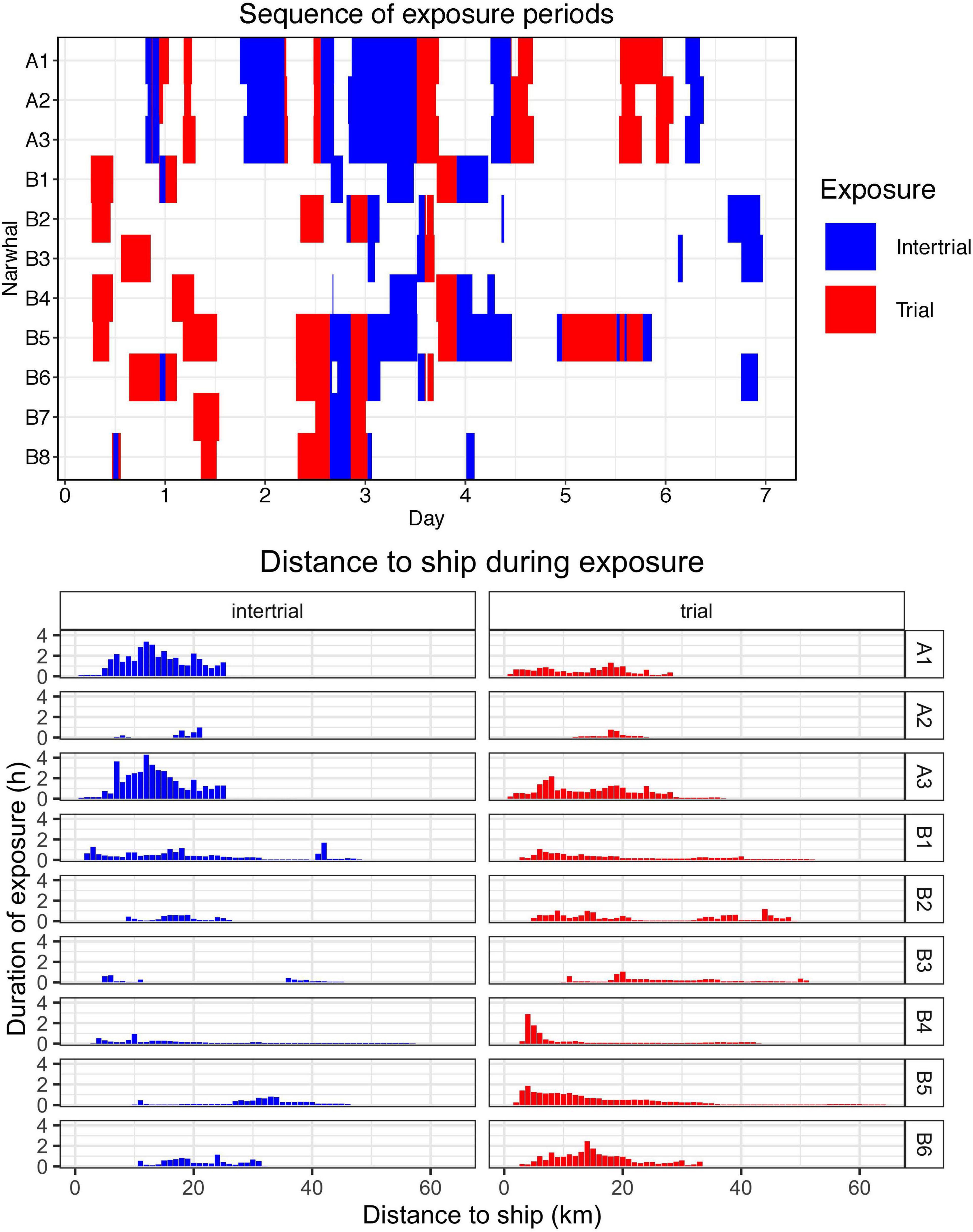
Figure 2. Upper panel The sequence of periods where each whale was exposed to the presence of the ship (intertrial) and seismic activity (trial) for the 11 whales with Fastloc or Fastloc CTD transmitters. Lower panel Duration (in hours) of exposure to the presence of the ship and seismic activity for the nine deployments with Acousonde recorders. Duration of exposure was calculated for 1-km bins.

Tracking of Narwhals and Seismic Effort

In 2017, the whales were primarily located in the western part of Gåsefjord during the period with seismic exposure (Figure 3). Over the course of 7 days, the seismic vessel conducted seven trials in that fjord with an active airgun and six intertrials with only the ship noise as exposure (Figure 2). The three Acousonde recorders that collected data during the study period lasted between 0.54 and 8.42 days.

FIGURE 3

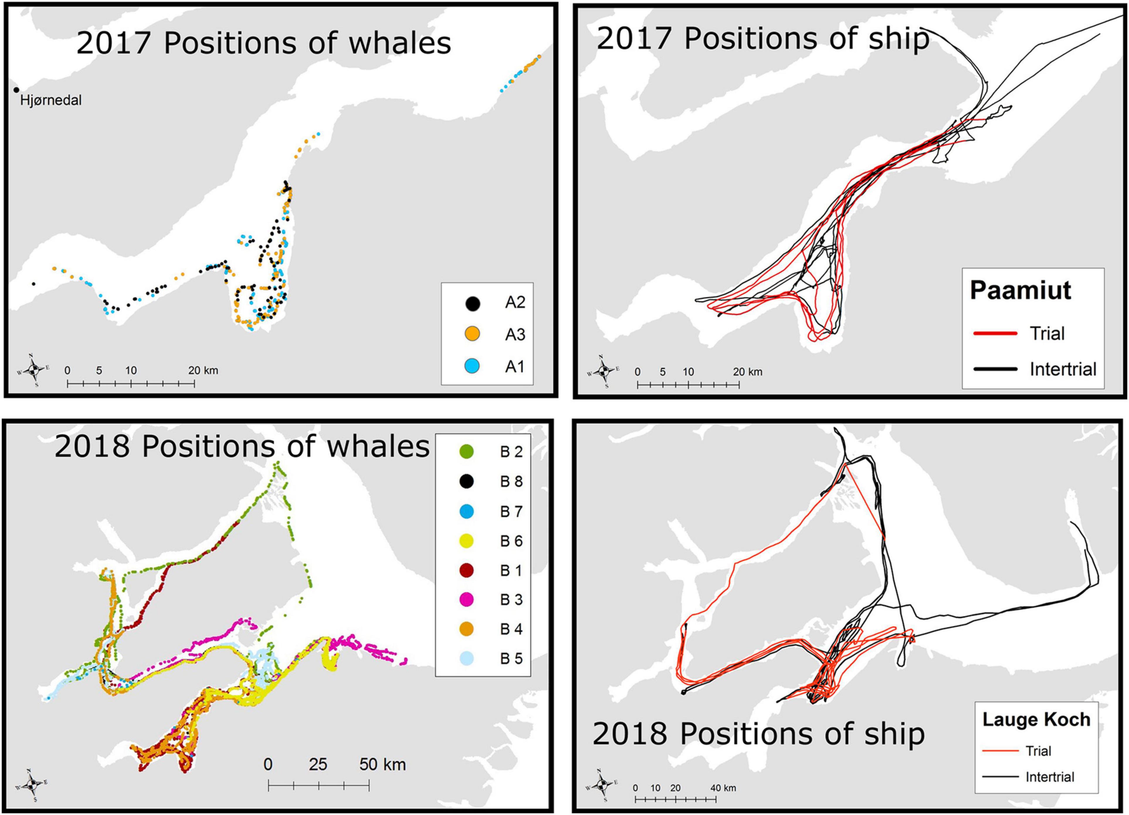
Figure 3. Upper panel, left Tracks of three whales subject to airgun trials between August 14 and 20, 2017 in Gåsefjord. Hjørnedal is the locality for the tagging of whales. Upper panel, right: Track of the seismic vessel r/v Paamiut in Outer Gåsefjord and in Gåsefjord (Figure 1). Red lines indicate effort with airgun shooting (trials), and black lines indicate effort without airgun activity (intertrials). Lower panel, left: Positions of eight narwhals tracked between August 24 and September 2, 2018 in Scoresby Sound. Lower panel, right: Positions of the seismic vessel HDMS Lauge Koch between August 24 and September 2, 2018 in Scoresby Sound. Red lines indicate periods with airgun shooting (trials), and black lines show periods without airgun activity.

In 2018, the tagged whales used a much larger part of Scoresby Sound (Figure 3). The seismic vessel performed eight trials over the course of 7 days, but none of the whales were exposed to more than five trials each. There were also up to 12 intertrials without an active airgun, but only eight had the whales within line of sight (Figure 2). The first two trials and several of the intertrials did not have any whales within line of sight. The six Acousonde deployments in 2018 lasted between 4.49 and 8.35 days, and all provided data during the period with exposure to airgun pulses.

Long-Term Movements of the Exposed Whales

The experimental exposure of the whales to airgun pulses and ship noise lasted 7 days each year, which is a relatively short exposure time compared to commercial seismic surveys. Nevertheless, it is important to test if any long-term effects of the disturbance of the whales can be detected. One option is to test if the whales exhibit changes in their migratory destinations. Previous studies have clearly delineated the winter ground for this population (cf. Heide-Jørgensen et al., 2015) and a comparison of the winter locations of exposed whales to tracks of unexposed whales from previous years suggest that there was no difference in the destination of the fall migration and the selection of winter ground (Figure 4). One whale tagged in August 2017 returned to the same area in August 2018 where it was tagged again and took part in the second seismic trial effort. This suggests that the whales were not abandoning the area after being exposed to the relatively low doses of sound from airgun pulses in 2017.

FIGURE 4

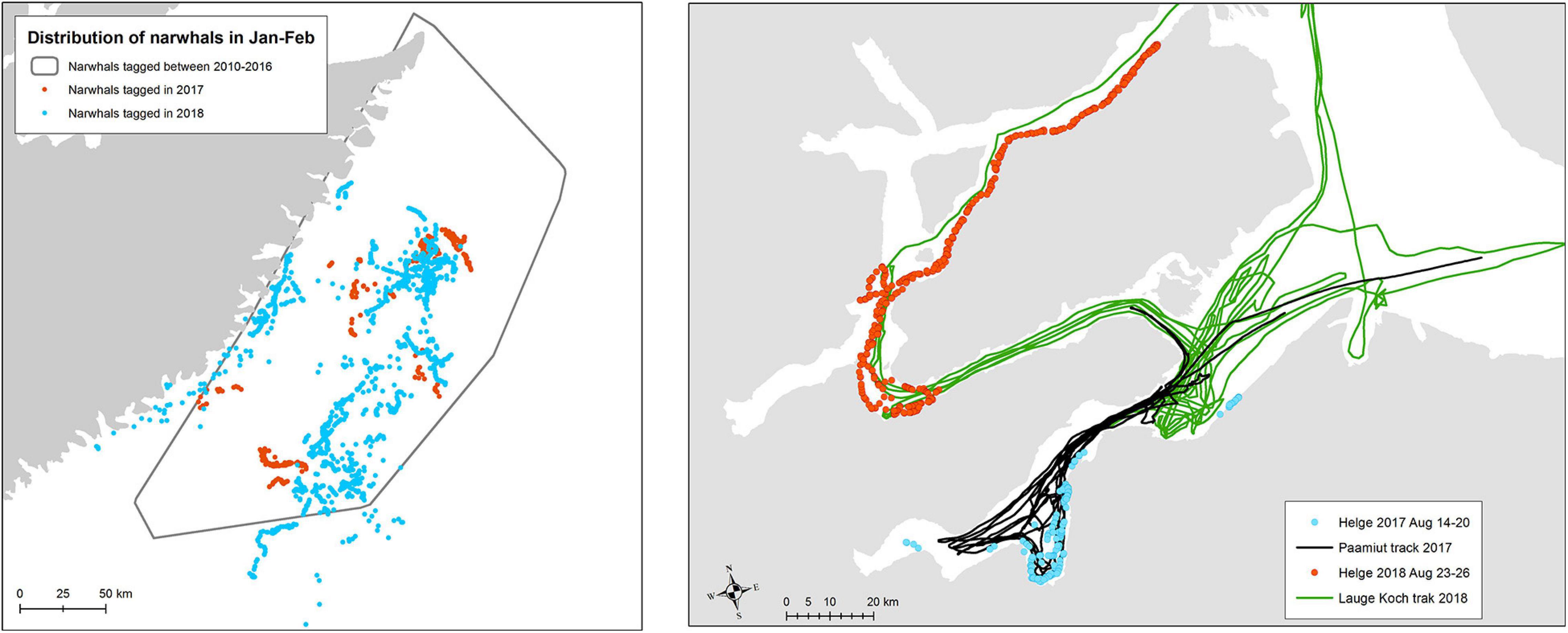
Figure 4. Left Winter positions of whales tracked in 2017 and 2018 during the winter months (January–February, n = 10) following exposure, compared to the minimum convex polygon of winter positions of 12 reference whales tracked in 2010–2016. Right Positions and exposure to seismic vessels of one whale (A1/B1) tagged in both 2017 and 2018.

Sound Levels From Airgun Pulses, MBES, 2018 Ship, and Background

Airgun pulse received SELs (unweighted), as collected during the SSVs, decreased rapidly with distance, and reached background about 3 km from the source for the small airgun and 8–10.5 km for the large airgun (10–10 kHz bandwidth, Figure 5A). The Supplementary Materials B–F include information on pulse durations, regression fits, as well as spectral density plots of the pulses for both sizes of airguns.

FIGURE 5

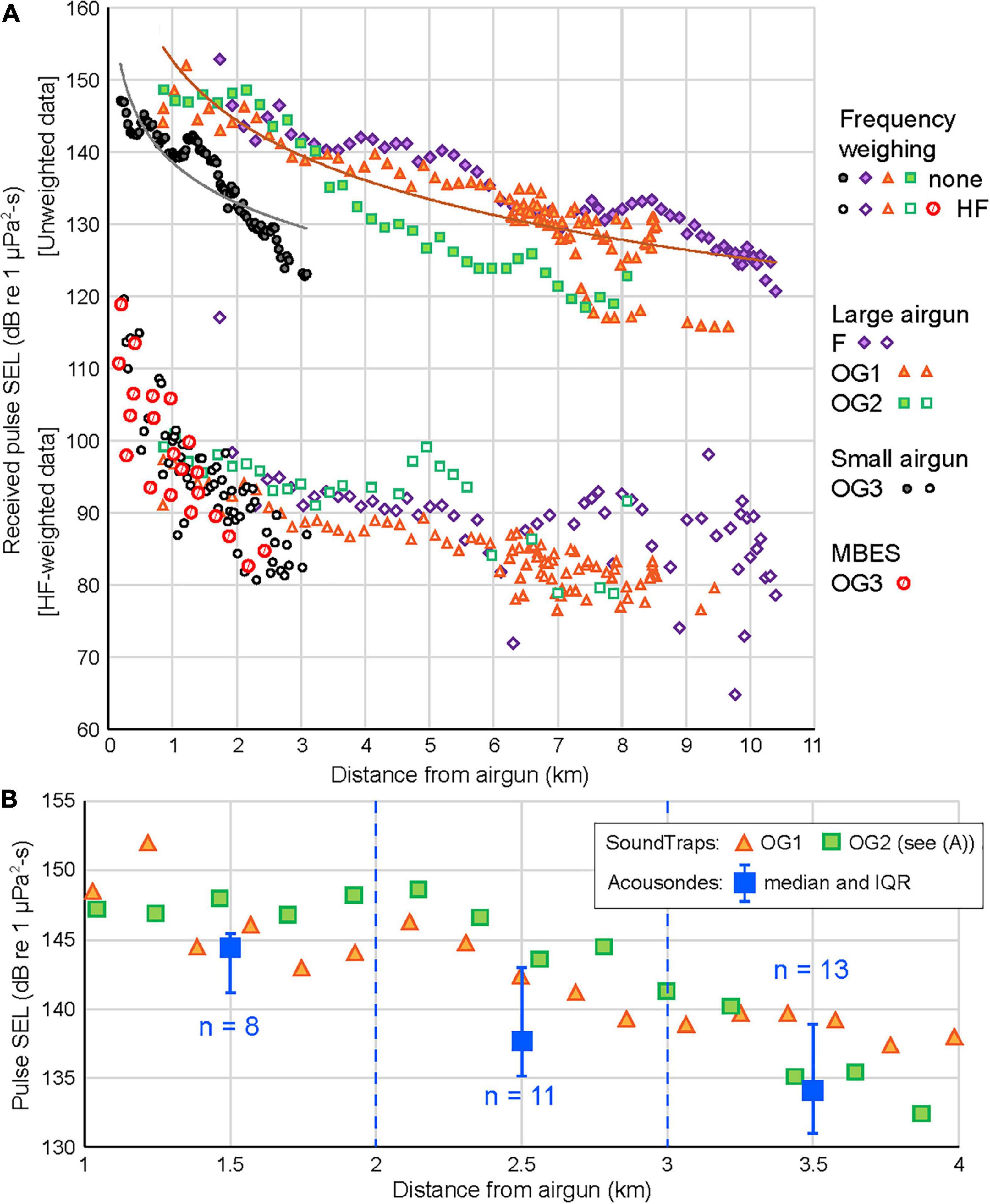
Figure 5. Received levels of sound from airgun pulses, as recorded (A) by SoundTraps during SSVs in Fønfjord (F), and Outer Gåsefjord (OG) at depths of 10 m. Unweighted (filled symbols) and HF-weighted (empty symbols) sound exposure level (SEL) as a function of distance for the small airgun (3.4 L or 210 in.³, black symbols) and large airgun (17.0 L or 1,040 in.³, colored symbols). The lines are logarithmic regressions through the data points for each gun size. Received HF-weighted SELs for pulses from the MBES are also shown. (B) Comparison of received unweighted SELs at SoundTraps [symbols as in panel (A)] with median levels (and IQRs) from whale-borne tags summarized for three 1-km bins, 1–4 km from the source. Acousonde data were from three whales (B1, B5, and B6); all data in panel (B) were collected in the Outer Gåsefjord (OG) area (Table 2).

To better assess actual sound levels received by the whales, received SELs (10–48 kHz) for the same pulses were computed after HF cetacean weighting (Southall et al., 2019, Figure 5A). The difficulty in analyzing these pulses and the fact that their RLs, when HF weighted, are below the background (see below) necessitate that they should be used qualitatively. Nevertheless, RLs for both airgun sizes show a decreasing trend with distance, out to about 6 km for pulses from the large airgun (Figure 5A).

Unweighted received SELs reported by Acousondes on three whales in Outer Gåsefjord (large airgun) were compared with the received SELs (also unweighted) obtained during two SSVs that were conducted in the same area in August 2018 (Table 2). Thirty-two pulses received by the whales at distances of 1–3.99 km from the airgun were grouped into three 1-km bins, and for each bin, the median (blue squares in Figure 5B) and interquartile range (IQR) (25th–75th percentile) are shown. The drifting SoundTraps collected data at a constant depth (10 m) in a situation essentially free of flow noise. In contrast, the Acousonde data were collected at a range of depths (1–45 m for the pulses shown) and included flow noise generated by the whales’ movements. This comparison (Figure 5B) shows that the two recording systems (SoundTraps and Acousondes), operating in dissimilar conditions (regarding depth and flow noise), obtained RLs with differences that can likely be attributed to the unfavorable signal-to-noise ratios (SNRs). Despite their shortcomings, the higher quality of the SSV data make them the best available estimates of sound levels received by the whales and will be used in that capacity for the remainder of this paper.

The Lauge Koch used a MBES to gather bathymetry data while in Scoresby Sound (2018). About every 1.4 s, the MBES produced a main pulse near 46.5 kHz and usually a secondary pulse near 23 kHz, both of which are roughly within the range of best hearing for HF cetaceans (see Supplementary Figures S7, S8 in Supplementary Materials C,D). The MBES was on during all SSVs and during trials and intertrials. Received SELs (90% energy approach, HF weighted) for 21 MBES pulses were analyzed as far away from the ship as possible, 2,430 m (Figure 5A). RLs showed a fair amount of variation, possibly due to the directionality of the echo sounder combined with the movements of the ship. Mean pulse duration was 0.75 s (SD, 0.26 s). HF-weighted SPLs for the highest-energy 200-ms segment of each of the analyzed pulses decreased from ∼125 dB re 1 μPa at a range of 170 to ∼90 dB re 1 μPa at 2,430 m.

Due to its duty cycle (on for ∼0.75 s every ∼1.4 s), both airgun pulse and background samples during HF-weighted airgun pulse analyses are likely to have included some variable amount of sound from the MBES. This may account for some of the variation in the values of the HF-weighted data compared to the unweighted data in Figure 5A.

Ship-generated (non-airgun) noise levels decreased logarithmically as a function of distance to Lauge Koch (Figure 6). These background levels provide information on ambient sound levels in Scoresby Sound in the ship’s absence, as well as on the ship’s noise contribution at short range. The distance at which unweighted RLs flattened out varied by SSV and depended on sea state and ice conditions. Generally, it was 3–6 km, and the farthest an analyst could hear the ship by listening to the recordings with headphones was ∼9.5 km. At ranges of 10–25.5 km from the vessel, ambient noise levels had a median value of 115.1 dB and an IQR of 112.4–117.2 dB re 1 μPa. Similarly, the HF-weighted data provided information on the presumed audibility of Lauge Koch to the whales’ ears. These sound levels flattened out at distances of 2.5–3.5 km (Figure 6) but were likely audible to a “HF-ear” beyond those distances. At a range of 10–25.5 km, median HF-weighted background levels were 95.0 dB with an IQR of 94.2–96.2 dB re 1 μPa. Note that no effort was made to include or exclude sounds from the MBES in the ship noise analyses.

FIGURE 6

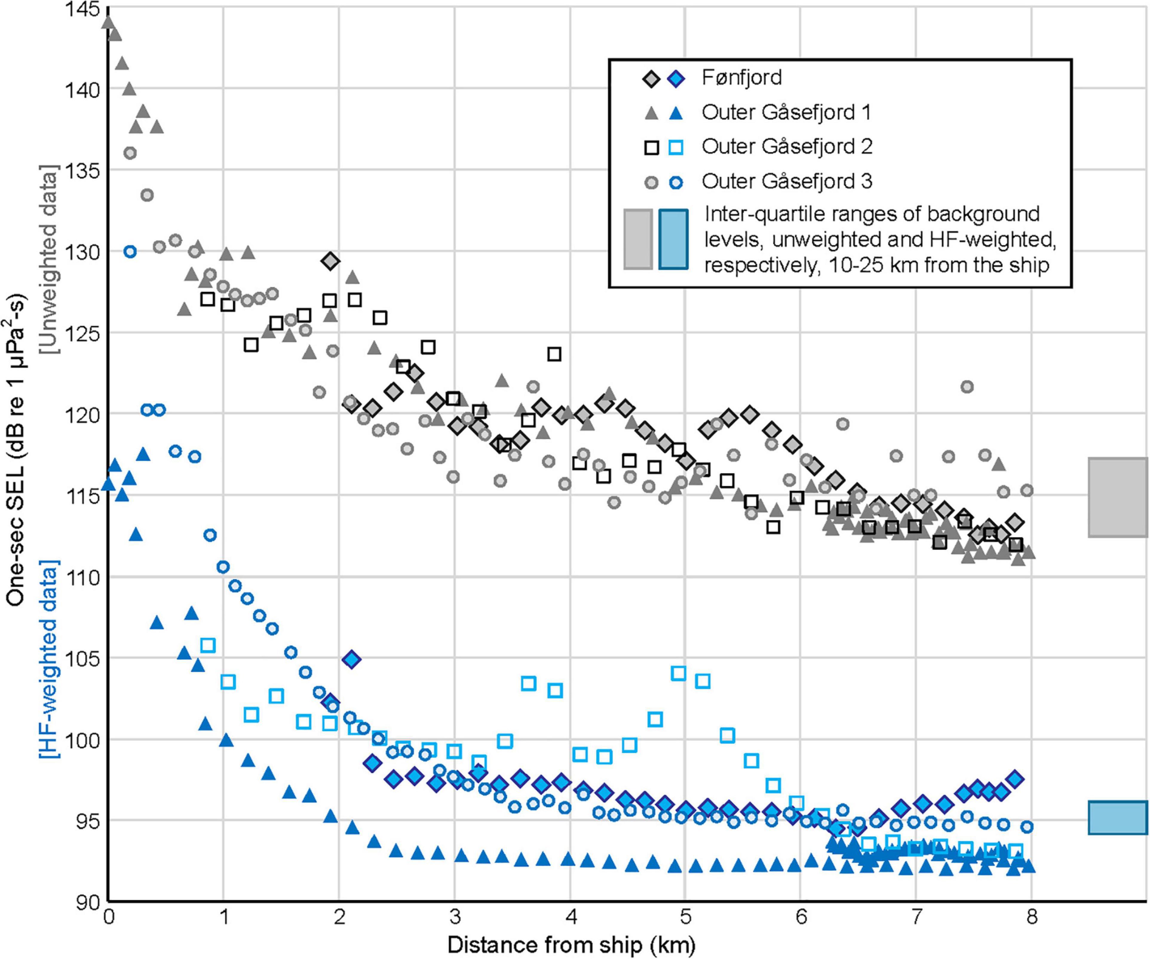
Figure 6. Broadband (10 Hz–48 kHz) background levels, unweighted (gray symbols) and HF-weighted (blue symbols), as collected during the four SSVs in Fønfjord and Outer Gåsefjord. Sample length is 1 s, so the values also correspond to sound pressure levels (SPL, in dB re 1 μPa). For comparison, the blocks on the right edge of the plot show the interquartile range (25th–75th percentiles) of background values analyzed 10–25.5 km from the ship.

In summary, despite the sounds produced by the MBES centered in the frequencies of best hearing of HF cetaceans, they decreased rapidly with distance in the HF-weighted data. It is somewhat unclear which of the sound sources (airgun pulses, MBES, and vessel itself) the whales were likely to better perceive a few kilometers from the ship, but it seems likely that airgun pulses were audible farther.

Immediate Effect of Sound Exposure on Animal Behavior

The whales clearly reacted to the presence of the seismic vessels both with and without the small or the large airgun. One example from August 18, 2017 showed three whales that were first exposed to airgun pulses at 10:56 at a distance of ∼6 km in Outer Gåsefjord (Figure 7A). They immediately headed north, then west around a peninsula at the entrance to Gåsefjord that may have masked the sound until ∼1.5 h later, when the vessel also passed the promontory and entered Gåsefjord. While maintaining a distance of 5–6 km, the whales kept heading west away from the vessel and into the inner part of the fjord where they remained even after the vessel had left the area. Another avoidance response can be seen in whale B6 that moved away from the ship’s area of operation (first track) and then returned (last track) as soon as the vessel left the area (Figure 7B).

FIGURE 7

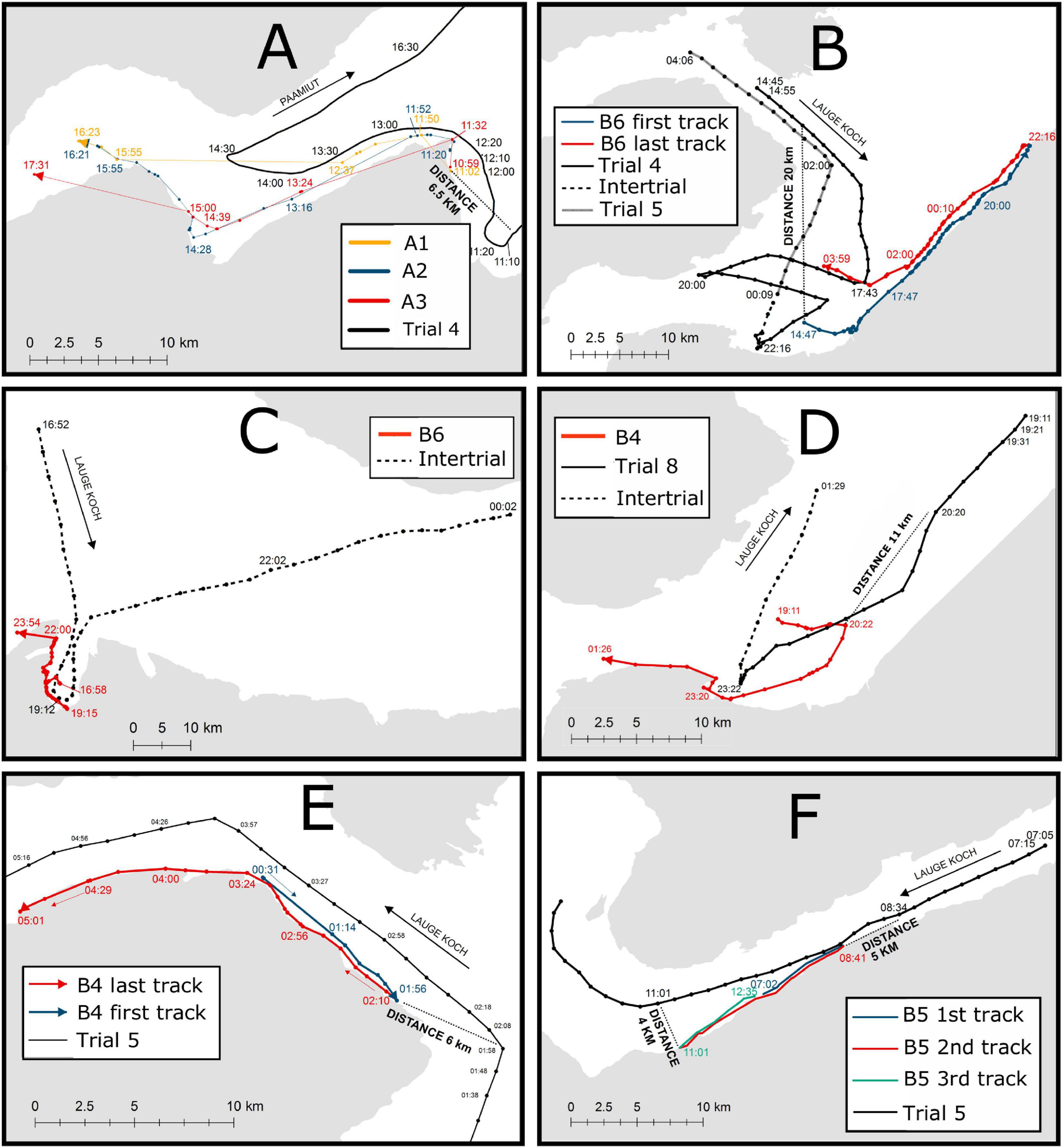
Figure 7. Whale track examples in the presence of approaching vessels, for three different contexts: whales offshore, nearshore, or in a cul-de-sac at the onset of exposure. (A) Three whales (A1, A2, and A3) near the coast on August 16, 2017. The whales were in Outer Gåsefjord when they first encountered the vessel at a distance of ∼6 km. They immediately headed north, then west into Gåsefjord, following the coast southwestward while trailed by the vessel, and continued into the inner part of Gåsefjord. (B) B6 offshore on August 26, 2018. The whale was in line of sight with the vessel at a distance of ∼24 km. It moved towards the shore and headed northeast away from the vessel. When 34 km from the vessel, it reversed direction and returned along the coast. At 02:00, when the vessel was ∼12 km away and receding, the whale headed offshore. (C) B6 in a cul-de-sac during an intertrial on September 1, 2018. The vessel was inside the bay between 18:12 and 20:32, and the whale remained close to the coast until it could leave the bay after 22:00. (D) B4 offshore on August 29, 2018. The whale was traveling east but moved south towards the coast when the vessel was ∼11 km from the whale. (E) B4 near the coast on August 27, 2018. The whale was first heading southeastward along the coast at 00:31, but at 01:56, it may have sensed the approaching vessel, which was then at a distance of 6 km. The whale then turned around and headed northwest, retracing its route while being followed by the vessel. (F) B5 near the coast on August 27, 2018. The whale was heading east but reversed course when the vessel was ∼5 km away. After the vessel passed the whale at a distance to the ship of ∼4 km, the whale reversed course again. The dotted lines indicate intertrials, and the full lines indicate trials.

When the whales were in a cul-de-sac situation, it was more difficult to detect a flight response. Whale B6, which was approached by the vessel without the airgun, remained close to the coast, eventually escaping from the cul-de-sac after the vessel had left (Figure 7C). While away from the coast, 11 km from the approaching ship, whale B4 reacted to the vessel by abruptly changing his direction of travel and heading towards the coast (Figure 7D).

An example from the 2018 experiment shows undisturbed whale B4 heading southeast at a speed of 1.60 m s^–1 (SD = 0.40 m s^–1) through Fønfjord until it was exposed to airgun pulses at 1:56 from Lauge Koch, which was entering Fønfjord in front of the whale, at a distance of ∼6 km (Figure 7E). The airgun pulses may not have been audible to the whale before it reached the easternmost point of Fønfjord where the vessel was in line of sight. The whale quickly turned around and headed back into Fønfjord where it traveled at an average speed of 1.97 m s^–1 (SD = 0.43 m s^–1) along the coast. After the vessel overtook the whale at 6:32 while traveling at a speed of 2.3 m s^–1 (SD = 0.15 m s^–1, not shown in Figure 7, see Supplementary Material G: Video Clip), the whale resumed travel to the east in Fønfjord at a slower speed of 1.50 m s^–1 (SD = 0.53 m s^–1). A similar episode happened to B5 while heading northeast along the coast during an approach by Lauge Koch. When the ship was ∼5 km away, the whale reversed direction, thereby traveling in the same direction as the ship. Once the ship had overtaken it, at a distance of ∼4 km, the whale reversed direction again and resumed its northeastward movement (Figure 7F).

From the tracks of the whales, it appeared that the whales concurrently moved away from the vessels and moved towards the shore during both trials and intertrials. We therefore decided to conduct detailed analyses of the horizontal speed of the whales as a disturbance effect.

The nine whales that provided Fastloc GPS positions during exposure situations were tagged on four different occasions, and some of them could be traveling together in a group. It was not possible to assess with certainty when whales were together, but it was assumed that individuals that were close to the coast during exposure events were with high probability traveling together. The pairwise comparison of the distance to coast was, therefore, tested with Pearson correlation coefficients, and it was obvious that the three whales tagged in 2017 were traveling as a group (Supplementary Table S1). This was also confirmed from mapping of their movements. In 2018, three of the six whales were simultaneously exposed for only some of the time; as a result, they were treated as independent samples.

The assumption that the whales only reacted to the active airgun when in line of sight was tested by comparing horizontal speeds during the 2-h pre-exposure periods for intertrials and trials. For the three context situations combined, the speed increased by 25% before the ship was in line of sight when both years were combined (Supplementary Table S2 in Supplementary Material E for details on the mixed-effect model). For the cul-de-sac and the inshore context, the speed increased significantly by 0.39 and 0.33 m/s, respectively. This could not be shown for the offshore context where the speed showed larger variability and decreased (by 17%). It confirms that the whales could indeed detect the noise from the airgun even when they were behind promontories or islands. This analysis, however, does not include the distance to the vessels, and because of the complex topography of the fjord system, there is no simple way to estimate the source range before the whales were in line of sight. Reverberations of airgun pulses in the fjord system make it even more difficult to estimate the exposure when the whales were not in line of sight. It was therefore decided to maintain the line-of-sight requirement for both intertrial and trial exposures.

In 2017, the three whales (A1–A3) were treated as one group. During intertrials in the cul-de-sac context, the travel speed of the group increased significantly (ANOVA p < 0.01) from 0.90 m/s during pre-exposure to 1.18 m/s during exposure (the intertrial itself), to 1.58 m/s during postexposure (Supplementary Table S3 in Supplementary Material E). During trials in the cul-de-sac context, the group speed was significantly lower (p < 0.01) during pre-exposure than exposure, but there was no significant change with the postexposure speed. Too few data were available for offshore trials and intertrials.

In 2018, when individual whales were in the cul-de-sac context, the horizontal speed increased significantly during and after intertrial exposures compared with the 2-h pre-exposure period (Figure 8, see Supplementary Table S4 in Supplementary Material E). This increase was evident in both years with the two vessel types. During trials in the cul-de-sac context in 2018, the speed declined significantly but not for the postexposure period. Significant increases in speed during and after exposure could also be detected for the inshore exposure during both trials and intertrials, but only for HDMS Lauge Koch in 2018 because no data were available from r/v Paamiut in 2017. For the offshore context, the speed also increased significantly during and after intertrials in 2018 but with opposite trend in 2017 during exposure. There was large variability in the speed of the whales during offshore trials, and no significant effect of exposure could be detected on the speed.

FIGURE 8

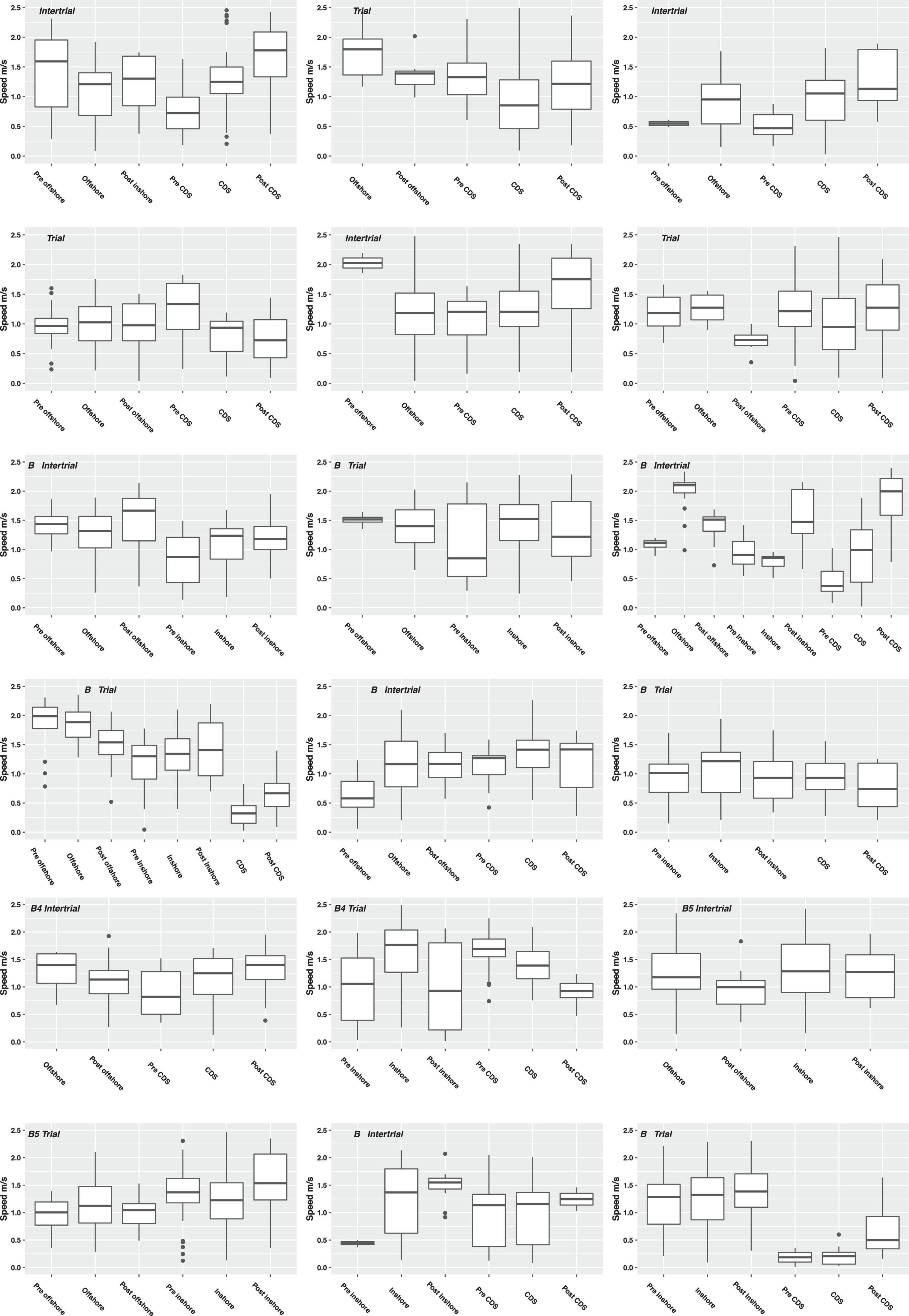
Figure 8. Boxplots of the horizontal speed of individual whales during intertrials (upper nine plots) and trials (lower nine plots) in different topographical context [inshore, offshore, or in cul-de-sac (CDS)]. The thick line in the middle is the median, the box identifies the first and third quantiles, the vertical line show the range of data, and dots indicate outliers.

One example of a whale (B1) from the 2018 experiment provides a good demonstration of the whales’ behavioral complexity (Figure 9). Before exposure to the vessel, the whale was off the coast, making foraging dives with buzzing activity to depths >400 m. This stopped during an intertrial period when the vessel approached the whale and the whale reacted by moving towards the coast. When the ship was no longer in line of sight, the whale resumed the offshore feeding dives. During the succeeding trial period, with airgun pulses initially at distances of >50 km, the whale started feeding offshore during the ship’s approach. It later started heading towards the coast when the ship was <30 km away and stopped feeding activity when the ship was <10 km away.

FIGURE 9

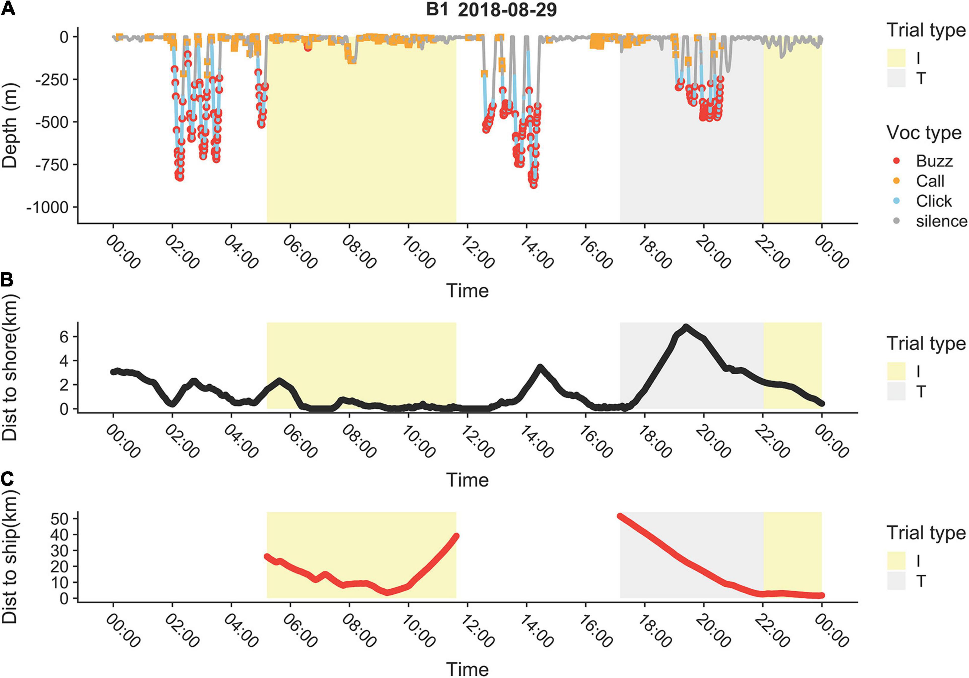
Figure 9. Example of storyboard with (A) diving and vocalization, (B) distance to coast, and (C) distance to ship during 1 day for one whale (B1) that was tagged in 2018. Trials (T) are shown in gray and intertrials (I) in yellow.

Distance to Shore

Exposure to seismic changed the amount of time spent close to shore (Supplementary Table S5 in Supplementary Material F), and the choice of threshold (150, 235, and 250 m) made no significant difference. In theory, the values at a threshold of 235 m should be around 5%; however, the reference whales were generally further away from the coast, whereas the whales that were exposed to seismic spent more time close to shore, within the threshold.

The estimated hazard ratios exp⁡(0.1β_jk) on each transition for an increase of 0.1 km^–1 in the exposure for the three distance-to-coast thresholds are shown in Figure 10. The hazard ratios for 0.1 increase are provided because the exposure typically varies between 0 and 1, so an increase of 1 is very large. A hazard ratio of 1 (i.e., β = 0) implies that there was no effect of exposure. A confidence interval that contains 1 means that the effect is not statistically significant. A hazard ratio < 1 means that the intensity of making that transition between states is smaller than during natural behavior, and a hazard ratio > 1 means that the intensity of making the transition between states is larger than during natural behavior. A hazard ratio of 1.3 means that the intensity of the transition is 30% higher if the exposure increases with 0.1. This cannot be directly translated to a distance to ship because of the nonlinear relation between exposure and distance to ship. The main conclusions are that increasing exposure increased the propensity of the whales to move towards and to remain close to shore, and decreased the probability of leaving the shore. This was most pronounced during the seismic experiment in 2018, when the intensity of moving from nearshore to offshore was highly unlikely.

FIGURE 10

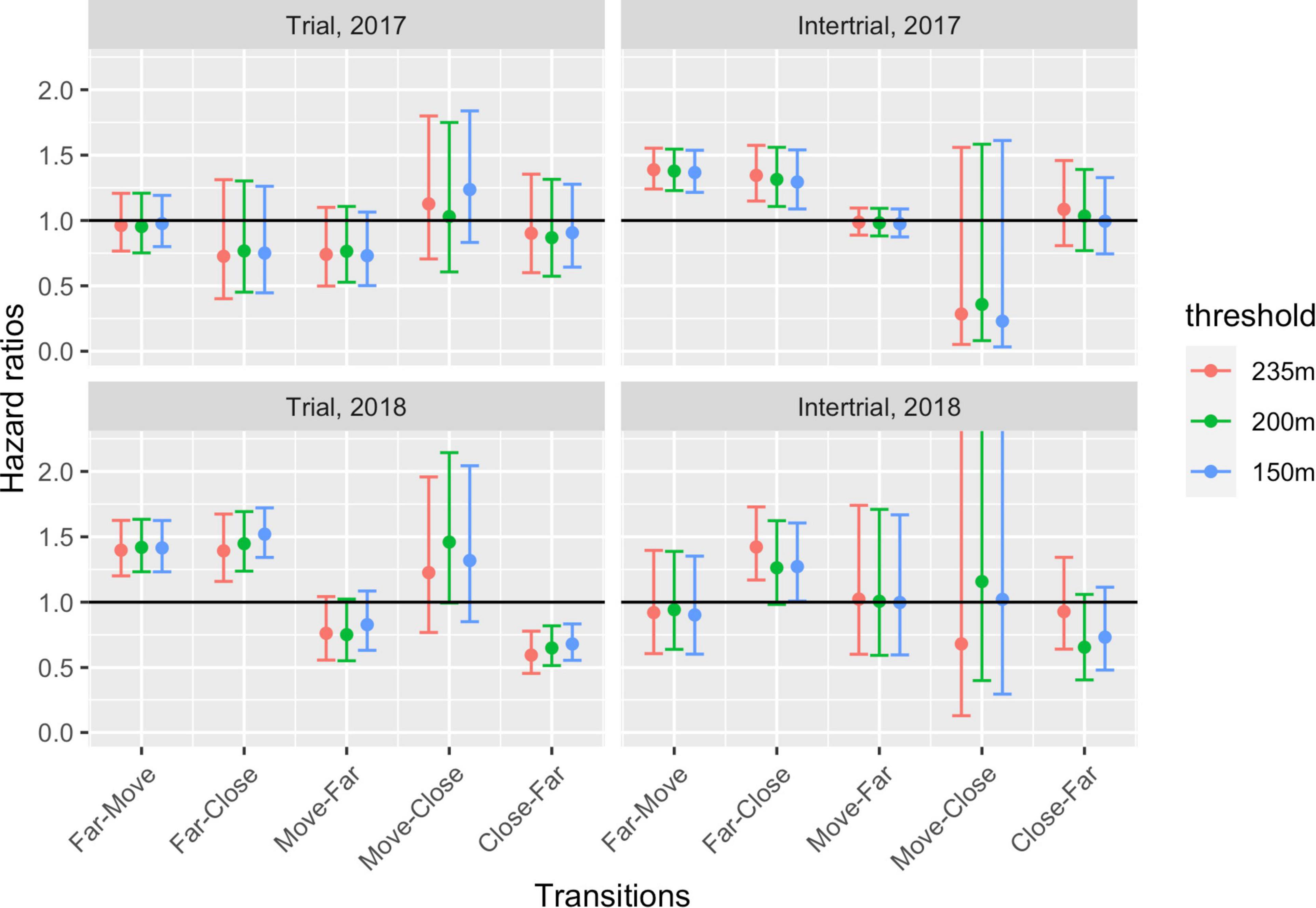
Figure 10. Estimated hazard ratios for an increase of 0.1 km^{− 1} in the exposure together with 95% confidence intervals for different threshold (150, 250, and 235 m from shore) under trials (seismic activity) and intertrials (presence of ship). The black horizontal lines at 1 indicates no effect of exposure.

During trials, there was an increasing probability that the whale would change state and move towards shore when the vessel approached (Figure 11). The most pronounced reaction occurred with the large airgun in 2018 where the propensity to dwell offshore was clearly diminished at distances of 15 km or more. The reaction to the vessels alone during intertrials occurred at exposure distances <10 km.

FIGURE 11

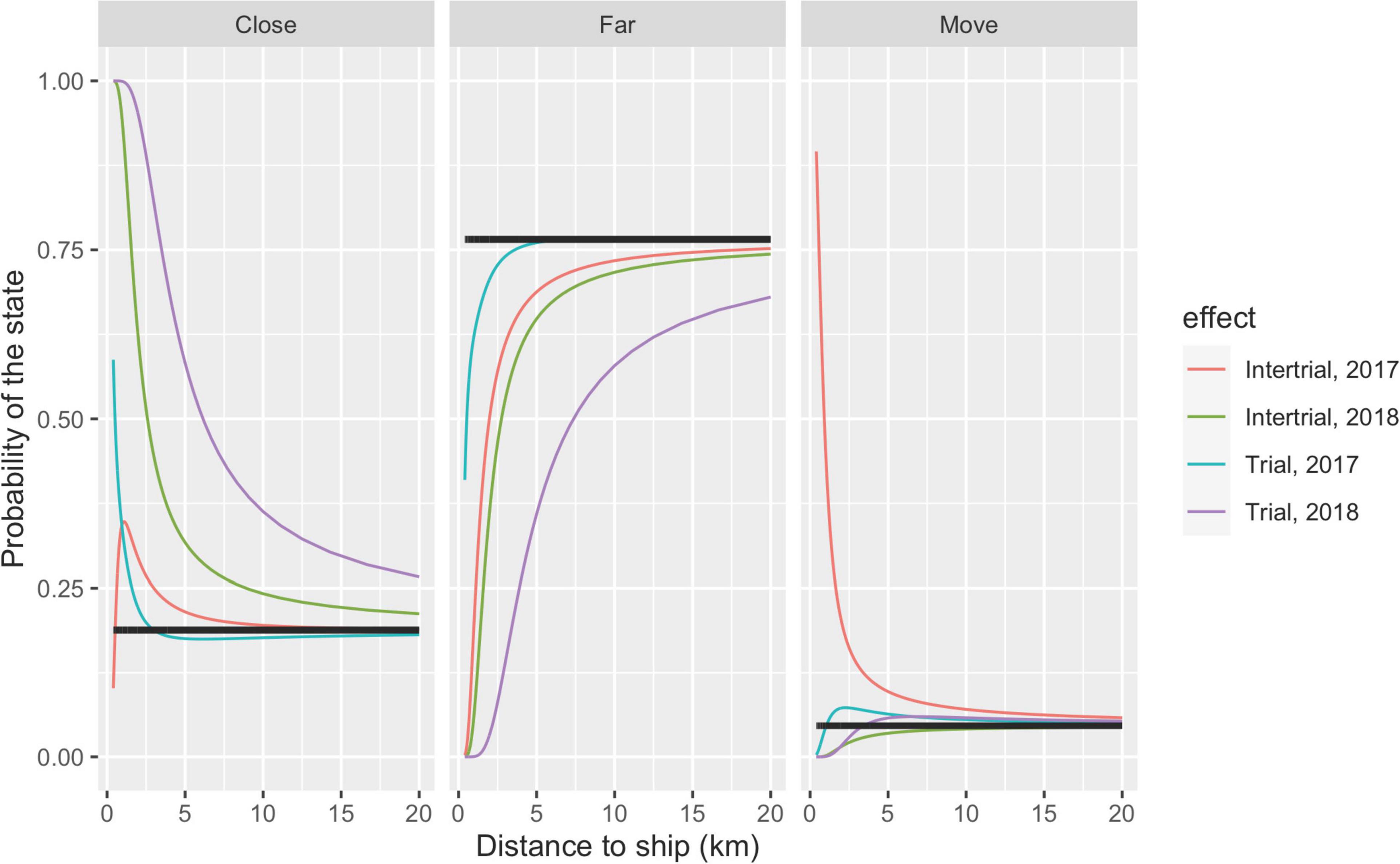
Figure 11. The three probabilities (Close, Far, and Move) as a function of distance to ship under trials (seismic activity, blue and pink curves for 2017 and 2018, respectively) and intertrials (presence of ship, red and green curves for 2017 and 2018, respectively). When the distance to ship goes to infinity (corresponding to no presence of ship), the distribution converges to the distribution under normal behavior; that is, the stationary distribution without exposure indicated by black lines. This distribution is Far = 0.760, Move = 0.049, and Close = 0.191 for the 235-m threshold between the states Far and Close. For example, at 20 km, there is still a considerable effect of exposure during trials in 2018, whereas for exposures in 2017, the undisturbed level is reached at a distance of 20 km. Note that the three curves of the same color in the three panels add to one.

To evaluate the effect of different exposure levels, we estimated the distance between the whale and ship at which the change in probability of being far from the coast was half that of normal behavior. We choose state 1 (far from the coast) because both states 2 and 3 (moving towards and being close to the coast) might indicate the same type of reactions to the exposures. Note that the probability of being in state 1 equals 1 minus the probability of being in either state 2 or 3. Under normal behavior (no exposure), the probability of being offshore without moving towards the coast was 0.76 for the 235 m threshold, i.e., on average, a narwhal spends 76% of its time more than 235 m from the coast. At ranges closer than the numbers given in Table 3, the whales, on average, spent less than half of their normal time (e.g., 76/2 = 38%) at distances beyond the threshold.

TABLE 3

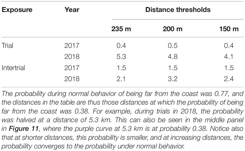
Table 3. Distance in kilometers at which the probability of being far from the coast was half of that seen during normal behavior for given exposures at three different thresholds of distance to coast.

Another way of measuring the effects of exposures was to look at the typical time that the whales stayed offshore before changing to any of the other two states (denoted sojourn time, Table 4). Under normal unexposed behavior, the whales stayed offshore for 68.7 min before changing state. This declined dramatically when the ship was moving closer to the whales, except for the trials in 2017 when the sojourn time increased, probably due to the whales being in an enclosed fjord.

TABLE 4

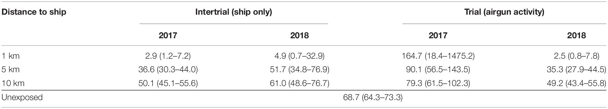
Table 4. Sojorn time, i.e., the average time (in min, with 95% confidence limits) that whales stayed far from the coast (in the Far state) before changing to any of the other two states, for normal unexposed behavior (bottom line) and for given distances to the ship under the four exposure levels.

Discussion

Direct studies of the effects of human activities on marine mammals are difficult to conduct because of the three-dimensional nature of their habitat, where detection of disturbance, reactions, and displacement are not easily observed. The use of animal-borne tags, however, offers possibilities for coupling detailed measurements of behavior with disturbance events in space and time. This study has focused on measurements of behavioral responses, primarily in terms of movements, of individual narwhals to variable doses of sound from a ship and its airguns during a sound exposure experiment using a suite of animal-borne recorders. The data from a large sample size of 11 exposed individuals clearly demonstrate that narwhals were affected by airgun pulses and even by ship presence without airgun activity at relatively long distances, particularly considering the short distance (<10 km) at which the sounds reached background levels. Generally, with decreasing range to sound sources, the whales tended to head towards the shore and stay near the shore, compared to normal behavior. In addition, when the whales were nearshore or in a cul-de-sac, they generally increased their travel speed during both trials and intertrials, except when in the presence of airgun pulses in the cul-de-sac, at which point they significantly decreased their travel speed.

Received Levels of Sounds

Unweighted RLs of sound from airgun pulses reached background at a distance of ∼3 km for the small airgun used in 2017 and 8–10.5 km for the large airgun used in 2018. At a distance of 10 km, unweighted received SELs for both airgun sizes were below 130 dB re 1 μPa² s (10 m depth).

Meanwhile, HF-weighted airgun pulse SELs were near or below background levels at all measured distances. These HF-weighted values should be used with caution due to the poor SNRs, but for the large airgun, they did, nevertheless, show a consistent decreasing trend out to about 6 km (Figure 5A).

Sounds from the MBES included higher frequency content than the airgun pulses (Supplementary Figures S7, S8 in Supplementary Materials C,D), thereby more closely matching the hearing sensitivity of an HF cetacean such as the narwhal. At close distances, e.g., <2 km, the MBES would have been the main sound source for an HF cetacean, since the much higher duty cycle of the MBES (over 80 s, ∼56 pulses vs. 1 pulse for the large airgun) would lead to much higher cumulative sound exposure levels (Southall et al., 2019). Nevertheless, encounters at those distances were rare (e.g., only one example with an active airgun at <2 km distance in 2018). In addition, the vessel and MBES sound sources decreased rapidly with distance and reached background <5 km from the source. It is therefore difficult to be certain which sound source the whales reacted to at short distances (<2 or 3 km) from the 2018 ship, particularly when one considers the additional variation added by depth and other factors of the propagation environment.

Avoidance reactions by the whales could be detected at distances >5 km from the source in 2017 and >11 km in 2018. There is little doubt that narwhals, despite masking by background noise, can sense anthropogenic activities at longer distances than what can be detected on the recordings. Finley et al. (1990) reported that narwhal and beluga (Delphinapterus leucas) reacted to low sound pressure levels (105 dB re 1 μPa) from icebreaking activities at distances of 40–60 km from the icebreaker. Presumably, detection distances were even larger. Cosens and Dueck (1993) confirmed that reaction distances of narwhals to ice-breaking activities at the ice edge in Lancaster Sound are within the same magnitude as reported by Finley et al. (op. cit.). Both studies were conducted in an offshore situation in partly ice-covered water where the whales could move away from the exposure. This is very different from the study in Scoresby Sound where the whales, due to the complex topography, were often exposed at shorter distances (i.e., 5–15 km) and usually within short distances of the coast. Maximum detection or reaction ranges could not be fully elucidated in this study because exposure at distances >50 km was seldom possible in the fjord system.

Reaction by the Whales: Change in Direction

Within the shorter exposure range in Scoresby Sound, the reaction of the whales could be detected at several levels. The most immediate response was the change in swimming direction in which the whales tried to avoid the sound source by changing the horizontal swimming direction and move close to the shore. Studies in Canada on the reaction of narwhals to the presence of killer whales (Orcinus orca) have shown that narwhals move within 500 m of the shore when killer whales are present (Laidre et al., 2006; Breed et al., 2017). This is in good agreement with the observations of movements in this study, and it was therefore natural to use “movements towards the coast” as a metric for the evasive response to exposure from ship or airgun noise. Other changes in horizontal movements as a reaction to the exposure are of course possible but are less discernible from normal behavior and more difficult to quantify.

The whales were clearly affected not only by ships using an airgun but also by ships alone. Even before the vessels, with an operating airgun, were within line of sight of the whales did the whales show a ∼30% increase in horizontal speed. This demonstrates the sensitivity of the whales to the airgun pulses, but the complex topography and the possibility for reverberations make it difficult to quantify the exposure level in situations when the whales were behind islands and promontories. Applying line of sight as the criterion for exposure evidently excludes some potential pre-response effects. Our estimates of effects must therefore be considered conservative with the obvious possibility that the effects could possibly be even larger.

The use of Markov models to analyze a possible flee and hide response of the narwhals to exposure is natural, since distance to coast observations are equally spaced in time, which is needed for the discrete time interpretations of transition probabilities, and furthermore measured at a time and space resolution that are sufficiently fine grained to capture the time and space scales of the responses. The Markov structure conveniently models the autocorrelations of the movement data. Covariates are easily included in the Markov models through the transition probabilities between states, such that the exposure is allowed to shape the behavioral response. Finally, standard software exists for the statistical analysis and estimation of the effect parameters. Hidden Markov models have been extensively used for the last decade to model biologging data of marine mammals, where different (unobserved) behavioral states that drive locomotion are modeled through hidden states. However, here, the behavioral drivers are the exposures, which are observed, leading to a fully observed Markov model and simplifying the analysis. In this paper, we chose a three-state Markov process: the two states close and far from shore and a “flee” state that allowed for traveling time from a position far from shore towards hiding close to shore. In this way, we were able to discern natural movement from the flee response when far from shore. The exposure was defined as a function of distance to ship for two reasons: first, because the exact sound exposure could not be precisely determined, due to the complicated topography and the low RLs of airgun pulses on the tags, and second because we believe that narwhals have a clear perception of the location of the threat (the ship), independently of the exact sound level, and thus, the distance to the ship may be a more important driver. The exposure should naturally be zero in the absence of a ship, and from zero, it should increase in a smooth and monotonic way as the ship approaches. Therefore, 1/distance was a natural choice, such that the exposure would decrease to zero continuously as the ship sailed away and increase to its maximum levels when the ship was on top of the animal. The monotonic shape ensures that if a certain threshold for the distance to ship is the trigger for a response, this will be captured, as will smoother responses, in which increasing exposure elicits an increasing response.

Reaction by the Whales: Change in Travel Speed

The Fastloc GPS receivers allowed for detailed tracks of each individual. The median time difference of only 5.0 min between subsequent GPS positions meant that a narwhal swimming at 1.5 m/s (the fastest horizontal swim speed calculated between subsequent positions <1 min apart) could travel 441 m between median-timed positions. This short time between positions and the slow speed of narwhals increases the accuracy of the constructed tracks and of the estimates of horizontal speed. During trials, narwhals tended to approach the coast (Figures 7, 10, 11), which could have negatively affected the ability of the Fastloc receivers to acquire GPS snapshots due to the steep mountain topography, sometimes exceeding 2,000 m, in the Scoresby Sound fjord system. However, we found that a slightly higher percentage (57% instead of 50%) of all surface periods with a duration of ≥4.2 s during trials had an associated GPS position. This could be due to a higher percentage of time spent at the surface during trials than in undisturbed situations. We therefore feel confident that the changes in the behavior of the whales, due to sound exposure, did not negatively bias the number of acquired positions. The accuracy of the interpretation of movements and the estimates of horizontal speed should therefore not have been affected by the exposure either. Due to the outstanding resolution in the movement data for each animal, we chose to approach the assessment of the effect of exposure using the distance between the animal and the sound source as the explanatory variable.

Depending on the context in which the whales were exposed, they usually increased their swimming speed to avoid the approaching sound source. Ship exposure in the cul-de-sac situation triggered a “flee response” (increased speed), but in the presence of the airgun (trials), the whales reduced their speed, and this “freeze response” may be an effect of the higher noise exposure initiated relatively close to the whales (<30 km and approaching). In the cul-de-sac situation, the whales moved towards or remained in close proximity to the shore. No effects of changes in speed could be detected in the offshore situations, but the whales generally moved towards the shore when the vessel was in the vicinity. This reaction was, however, less obvious when the whales already were inshore. The propensity of the whales to leave the inshore areas decreased with the proximity of the vessel. For the large airgun used in 2018, the whales reacted by moving towards the coast at distances of 10–15 km. A shorter reaction distance could be seen with the smaller airgun and with the vessels without an active airgun. Finley et al. (1990) described both a “flee” and a “freeze” response of narwhals in response to an icebreaker, and this has also been observed when narwhals are exposed to threats from killer whales (Laidre et al., 2006). The potential switching between the two behavioral states complicates the statistical detection of a movement response, as the whales can both stop or increase their speed and move or remain still in the same segment of the exposure. Instead, analyses of the vocal and dive responses are required to estimate the maximum distance for detection and reactions of the whales.

Reactions to anthropogenic sounds such as avoidance and increases in travel speed have been reported in other behavioral response studies (although to our knowledge, the reaction of heading towards shore has not). In response to navy sonar, beaked whales moved away from the source of the sound (Tyack et al., 2011) while also increasing their speed (DeRuiter et al., 2013; Wensveen et al., 2019). Dunlop et al. (2018) also report avoidance behavior by humpback whales (Megaptera novaeangliae) subjected to airgun pulses, although the responses described were multifaceted. For example, at the higher airgun pulse RLs, the probability of a response (moving away and increasing travel speed) actually decreased.

Background Level and Propagation Considerations

The Atlantic Arctic generally has lower background noise levels at low frequencies compared to equatorial regions (Haver et al., 2017). This is mainly due to the dampening effect of seasonal ice cover on wave action, but during summer, after the noisy melting and disintegration of sea ice, offshore Arctic background noise levels increase due to wind, rain, and anthropogenic activities (Klinck et al., 2012). Inside fjord systems, where narwhals are found in summer, wave height is lower, and hence, the main sources of background noise, away from glacial fronts, are from the breakup of icebergs, sporadic sound sources that the whales are familiar with. New sounds introduced by anthropogenic activities are therefore likely easily detected by the whales. The background noise levels recorded in this study in Scoresby Sound in summer were higher than levels measured at the ice edges of Lancaster Sound (93–104 dB re 1 μPa in the 10–1,000-Hz band) and Admiralty Inlet (85–92 dB re 1 μPa in the 10–1,000-Hz band) in spring (Finley et al., 1990; Cosens and Dueck, 1993). The background noise levels in Scoresby Sound were also higher than at the narwhals’ winter ground in the dense pack ice in northern Baffin Bay and at a summer ground in Northwest Greenland (Thiele, 1982, 1983). Apparently, narwhals winter in offshore areas where background noise levels are low due to ice coverage. During ice breakup, they abandon the increasingly noisy offshore areas and move into summer grounds with presumably lower noise level.

Underwater sound propagation is complex, especially close to the surface and in the Arctic (Urick, 1983). The presence of drifting ice, both sea ice and freshwater icebergs, creates local variations in acoustic properties in addition to being physical obstacles inducing shadow effects, especially for high frequencies. Furthermore, complex vertical and horizontal reverberation patterns further complicate the near-surface sound propagation. A confounding factor in the Arctic is the possibility for entrapment and long-range propagation of sounds in the upper part of the water column above distinct oceanographic layers. This phenomenon may greatly enhance the propagation of signals, making them audible to the whales over vast distances. While this has not been observed directly in this study, it may occur, as thermo- and haloclines exist at <10 m depth and, albeit weaker, at 100 m depth in Scoresby Sound (Heide-Jørgensen et al., 2020).

Agreement With Past Studies

The long reaction distance (>11 km), and presumably even longer detection distance, of narwhals agrees with the lack of sightings of narwhals by marine mammal observers onboard seismic vessels conducting industrial-scale exploratory surveys (Lang and Mactavish, 2011; Vanman and Durinck, 2012; Frouin-Mouy et al., 2017). Narwhals are also considered very skittish and hard to approach by many Inuit hunters, and hunting and harpooning them from silently moving kayaks is the preferred hunting method in many areas of Greenland (Heide-Jørgensen, 1994). Based on a propagation model, Schack and Haapaniemi (2017) estimated that belugas, a close relative of narwhals, could potentially detect ship noise (container vessel and icebreaker) up to a distance of 50 km during the ice-covered season and at even longer distances in open water. Apparently, narwhals react to anthropogenic exposure at much longer distances than most other odontocetes (Davis et al., 1991), and this may either be because the whales are adapted to an environment with relatively low and well-known background noise levels and/or because narwhals are particularly naive to anthropogenic activities due to the remote and inaccessible areas they inhabit.

Cumulative Effects

This study does not address the effects on narwhals of long-term exposure from industrial-scale seismic surveys and continued ship traffic. The possibility of long-term habituation and recovery from continued anthropogenic disturbances also needs to be addressed in studies conducted over longer time scales. The effects detected in this study are pronounced and detectable even at long distances (>11 km) from the source. Narwhals exhibit strong site fidelity, have well-defined migratory routes, and show limited plasticity in dispersal patterns (Heide-Jørgensen et al., 2003, 2015). This, combined with the fact that they are relatively naive to anthropogenic activities, definitely makes them vulnerable to the introduction of noise pollution in their remote and pristine habitats.

Finally, and importantly, it can be assumed that the level of exposure in these experiments, both in terms of the duration of the experiment and the RLs of airgun pulses, did not harm the whales or cause long-term behavioral changes. One whale first captured and tagged in 2017 returned to the same area the following year where it was tagged again, still in good condition. In both years, the fall migratory destination and winter ground were similar to those of unexposed whales tracked in previous years. Extreme site fidelity has been observed before for this population (Heide-Jørgensen et al., 2015), and it seems to be maintained despite the disturbance. Low behavioral flexibility and lack of alternative habitats may, however, also explain why, in the fall, after leaving the fjord system where they were exposed to the airgun pulses, all the whales chose the very same winter ground that has been used by narwhals from this population for the past decade.

Data Availability Statement

The raw data supporting the conclusions of this article will be made available by the authors, without undue reservation.

Ethics Statement

The animal study was reviewed and approved by the Institutional Animal Care and Use Committee of the University of Copenhagen (17 June 2015).

Author Contributions

MH-J, SB, and TW contributed to the conception and design of the study. MH-J, OT, RH, HS, M-HS, TW, and SB conducted the field work with live capturing of the whales. PT, EG, MN, and SB conducted the seismic trials. SD, AS, MN, OT, RH, and MH-J analyzed the location and behavioral data and SB and AC analyzed the acoustic data. MH-J wrote the first draft of the manuscript. All authors contributed to the manuscript revision, read, and approved the submitted version.

Funding

The Mineral Licence and Safety Authority (MLSA) and Environmental Agency for Mineral Resource Activities (EAMRA) of Greenland provided funding as part of the Joint Northeast Greenland Strategic Environmental Study Program. Additional funding was obtained from the Carlsberg Foundation and the Danish Cooperation for the Environment in the Arctic (DANCEA). Permission for capturing, handling, and tagging of narwhals was provided by the Government of Greenland (Case ID 2010 ± 035453, document number 429 926). The project was reviewed and approved by the IACUC of the University of Copenhagen (June 17, 2015). Access and permits to use land facilities in Scoresby Sound were provided by the Government of Greenland. No protected species were sampled.

Conflict of Interest

SB was employed by the company Greeneridge Sciences Inc.

The remaining authors declare that the research was conducted in the absence of any commercial or financial relationships that could be construed as a potential conflict of interest.

Acknowledgments

We thank the hunters from Ittoqqortoormiit for their assistance in catching the whales and in deploying and collecting instruments; we are particularly indebted to Inuuta Scoresby Hammeken, who facilitated a major part of the field operations. The crews of r/v Paamiut and HDMS Lauge Koch are acknowledged for their skillful navigation in Scoresby Sound. Mikkel Skovrind, Jeppe Møhl, Mads Fage Christoffersen, Sixten Hüllert, Solveig Heide-Jørgensen, Alice Hüllert, and Beau Richter are thanked for their help with field logistics, camp maintenance, and capturing operations in Hjørnedal. Lars Mejlgaard Rasmussen and Andreas Skifter Madsen, Aarhus University, are thanked for their assistance with seismic operations onboard r/v Paamiut and HDMS Lauge Koch. This study is part of the Northeast Greenland Environmental Study Program, which is a collaboration between DCE–Danish Centre for Environment and Energy at Aarhus University, the Greenland Institute of Natural Resources, and the Environmental Agency for Mineral Resource Activities of the Government of Greenland. Oil companies operating in Greenland are obliged to contribute to knowledge regarding environmental matters.

Supplementary Material

The Supplementary Material for this article can be found online at: https://www.frontiersin.org/articles/10.3389/fmars.2021.658173/full#supplementary-material

Footnotes

1. ^ www.acousonde.com

References

Ahonen, H., Stafford, K. M., de Steur, L., Lydersen, C., Wiig, Ø, and Kovacs, K. (2017). The underwater soundscape in western Fram Strait: breeding ground of Spitsbergen’s endangered bowhead whales. Mar. Polut. Bull. 123, 97–112. doi: 10.1016/j.marpolbul.2017.09.019

PubMed Abstract | CrossRef Full Text | Google Scholar

Andrews, R. D., Baird, R., Calambokidis, J., Goertz, C. E. C., Gulland, F., Heide-Jørgensen, M. P., et al. (2019). Best practice guidelines for cetacean tagging. J. Cetacean Res. Manag. 20, 27–66.

Google Scholar

Bernaldo de Quirós, Y., Fernandez, A., Baird, R. W., Brownell, R. L. Jr., Aguilar de Soto, N., Allen, D., et al. (2019). Advances in research on the impacts of anti-submarine sonar on beaked whales. Proc. R. Soc. B 286:20182533. doi: 10.1098/rspb.2018.2533

PubMed Abstract | CrossRef Full Text | Google Scholar

Blackwell, S. B., Lawson, J. W., and Williams, M. T. (2004). Tolerance by ringed seals (Phoca hispida) to impact pipe-driving and construction sounds at an oil production island. J. Acoust. Soc. Am. 115, 2346–2357. doi: 10.1121/1.1701899

CrossRef Full Text | Google Scholar

Blackwell, S. B., Tervo, O. M., Conrad, A. S., Sinding, M.-H. S., Hansen, R. G., Ditlevsen, S., et al. (2018). Spatial and temporal patterns of sound production in East Greenland narwhals. PLoS One 13:e0198295. doi: 10.1371/journal.pone.0198295

PubMed Abstract | CrossRef Full Text | Google Scholar

Boertmann, D., Blockley, D., and Mosbech, A. (2020). Greenland Sea–An Updated Strategic Environmental Impact Assessment of Petroleum Activities Scientific Report from DCE–Danish Centre for Environment and Energy No. 375. Roskilde: Nationalt Center for Miljø Og Energi, 380.

Google Scholar

Breed, G. A., Matthews, C. J., Marcoux, M., Higdon, J. W., LeBlanc, B., Petersen, S. D., et al. (2017). Sustained disruption of narwhal habitat use and behavior in the presence of Arctic killer whales. Proc. Natl. Acad. Sci. U.S.A. 114, 2628–2633. doi: 10.1073/pnas.1611707114

PubMed Abstract | CrossRef Full Text | Google Scholar

Bröker, K. C. (2019). An overview of potential impacts of hydrocarbon exploration and production on marine mammals and associated monitoring and mitigation measures. Aquat. Mamm. 45, 576–611. doi: 10.1578/AM.45.6.2019.576

CrossRef Full Text | Google Scholar

Bryant, E. (2007). 2D Location Accuracy Statistics for Fastloc§Cores Running Firmware Versions 2.2 & 2.3. Washington, DC: Wildtrack Telemetry Systems Ltd.

Google Scholar

Chambault, P., Tervo, O. M., Garde, E., Hansen, R. G., Blackwell, S. B., Williams, T. M., et al. (2020). The impact of rising sea temperatures on an Arctic top predator, the narwhal. Sci. Rep. 10:18678. doi: 10.1038/s41598-020-75658-6

PubMed Abstract | CrossRef Full Text | Google Scholar

Cosens, S. E., and Dueck, L. P. (1993). Icebreaker noise in lancaster sound, N.W.T., Canada: implications for marine mammal behavior. Mar. Mamm. Sci. 9, 285–300. doi: 10.1111/j.1748-7692.1993.tb00456.x

CrossRef Full Text | Google Scholar

Davis, R. A., Richardson, W. J., Thiele, L., Dietz, R., and Johansen, P. (1991). “Report on underwater noise,” in The State of the Arctic Environment Reports (Rovaniemi: University of Lapland), 154–269.

Google Scholar

DeRuiter, S. L., Southall, B. L., Calambokidis, J., Zimmer, W. M. X., Sadykova, D., Falcone, E. A., et al. (2013). First direct measurements of behavioural responses by Cuvier’s beaked whales to mid-frequency active sonar. Biol. Lett. 9:20130223. doi: 10.1098/rsbl.2013.0223

PubMed Abstract | CrossRef Full Text | Google Scholar

Dietz, R., Heide-Jørgensen, M. P., Richard, P., Orr, J., Laidre, K., and Schmidt, H. C. (2008). Movements of narwhals (Monodon monoceros) from admiralty inlet monitored by satellite telemetry. Polar Biol. 31, 1295–1306. doi: 10.1007/s00300-008-0466-4

CrossRef Full Text | Google Scholar

Digby, P. S. B. (1953). Plankton production in scoresby sound, East Greenland. J. Anim. Ecol. 22, 289–322. doi: 10.2307/1818

CrossRef Full Text | Google Scholar

Dunlop, R. A., Noad, M. J., McCauley, R. D., Kniest, E., Slade, R., Paton, D., et al. (2018). A behavioural dose-response model migrating humpback whales and seismic airgun noise. Mar. Pollut. Bull. 133, 506–516. doi: 10.1016/j.marpolbil.2018.07.009

CrossRef Full Text | Google Scholar

Dunlop, R. A., Noad, R. M. J., McCauley, D., Scott-Hayward, L., Kniest, E., Slade, R., et al. (2017). Determining the behavioural dose-reponse relationship of marine mammals to airgun noise and sound proximity. J. Exp. Biol. 220, 2878–2886. doi: 10.1242/jeb.160192

PubMed Abstract | CrossRef Full Text | Google Scholar

Elliott, B. W., Read, A. J., Godley, B. J., Nelms, S. E., and Nowacek, D. P. (2019). Critical information gaps remain in understanding impacts of industrial seismic surveys on marine vertebrates. Endanger. Species Res. 39, 247–254. doi: 10.3354/esr00968

CrossRef Full Text | Google Scholar

Finley, K. J., Miller, G. W., Davis, R. A., and Greene, C. R. (1990). Reactions of belugas, (Delphinapterus leucas) and narwhals, (Monodon monoceros) to ice-breaking ships in the Canadian high arctic. Can. Bull. Fish. Aquat. Sci. 224, 97–117.

Google Scholar

Frouin-Mouy, H., Kowarski, K., Martin, B., and Bröker, K. (2017). Seasonal trends in acoustic detection of marine mammals in Baffin Bay and Melville Bay, Northwest Greenland. Arctic 70, 59–76. doi: 10.14430/arctic4632

CrossRef Full Text | Google Scholar

Garde, E., Heide-Jørgensen, M. P., Ditlevsen, S., Tvermosegaard, K. T., Harding, K., Hansén, J., et al. (2015). Population dynamics of narwhals Monodon monoceros from East and West Greenland. J. Mammal. 96, 866–879. doi: 10.1093/jmammal/gyv110

CrossRef Full Text | Google Scholar

Graham, I. M., Merchant, N. D., Farcas, A., Barton, T. R., Cheney, B., Bono, S., et al. (2019). Harbour porpoise responses to pile-driving diminish over time. R. Soc. Open sci. 6:190335. doi: 10.1098/rsos.190335

PubMed Abstract | CrossRef Full Text | Google Scholar

Haver, S. M., Klinck, H., Nieukirk, S. L., Matsumoto, H., Dziak, R. P., and Miksis-Olds, J. L. (2017). The not-so-silent world: measuring Arctic, Equatorial, and Antarctic soundscapes in the Atlantic Ocean. Deep Sea Res. 1: Oceanogr. Res. Pap. 122, 95–104. doi: 10.1016/j.dsr.2017.03.002

CrossRef Full Text | Google Scholar

Heide-Jørgensen, M. P. (1994). Distribution, exploitation and population status of white whales (Delphinapterus leucas) and narwhals (Monodon monoceros) in West Greenland. Meddr Grønland 39, 135–149.

Google Scholar

Heide-Jørgensen, M. P., Blackwell, S. B., Williams, T. M., Sinding, M.-H. S., Skovrind, M., Tervo, O. M., et al. (2020). Some like it cold: temperature dependent habitat selection by narwhals. Ecol. Evol. 10, 8073–8090. doi: 10.1002/ece3.6464

PubMed Abstract | CrossRef Full Text | Google Scholar

Heide-Jørgensen, M. P., Dietz, R., Laidre, K., Schmidt, H. C., Richard, P., and Orr, J. (2003). The migratory behaviour of narwhals (Monodon monoceros). Can. J. Zool. 81, 1298–1305. doi: 10.1139/z03-117

PubMed Abstract | CrossRef Full Text | Google Scholar

Heide-Jørgensen, M. P., Hansen, R. G., Westdal, K., Reeves, R. R., and Mosbech, A. (2012). Narwhals and seismic exploration: is seismic noise increasing the risk of ice entrapments? Biol. Conserv. 158, 50–54. doi: 10.1016/j.biocon.2012.08.005

CrossRef Full Text | Google Scholar

Heide-Jørgensen, M. P., Nielsen, N. H., Hansen, R. G., and Blackwell, S. (2014). Stomach temperature of narwhals (Monodon monoceros) during feeding events. Anim. Biotelem. 2:9. doi: 10.1186/2050-3385-2-9

CrossRef Full Text | Google Scholar

Heide-Jørgensen, M. P., Nielsen, N. H., Hansen, R. G., Schmidt, H. C., Blackwell, S. B., and Jørgensen, O. A. (2015). The predictable narwhal: satellite tracking shows behavioural similarities between isolated subpopulations. J. Zool. 297, 54–65. doi: 10.1111/jzo.12257

CrossRef Full Text | Google Scholar

Hildebrand, J. A. (2005). “Impacts of anthropogenic sound,” in Marine Mammal Research: Conservation beyond Crisis, eds J. E. Reynolds, W. F. Perrin, R. R. Reeves, S. Montgomery, and T. J. Ragen (Baltimore, MD: The Johns Hopkins University Press), 101–124.

Google Scholar

Hildebrand, J. A. (2009). Anthropogenic and natural sources of ambient noise in the ocean. Mar. Ecol. Prog. Ser. 395, 5–20. doi: 10.3354/meps08353

CrossRef Full Text | Google Scholar

Hobbs, R. C., Reeves, R. R., Prewitt, J. S., Desportes, G., Breton-Honeyman, K., Christensen, T., et al. (2019). Global review of the conservation status of monodontid stocks. Mar. Fish. Rev. 81, 1–41.

Google Scholar

Jackson, C. H. (2011). Multi-state models for panel data: the msm package for R. J. Stat. Softw. 38, 1–29.

Google Scholar

Jepsen, H. F., Ineson, J. R., Mikkelsen, N., Piasecki, S., Platen-Hallermund, F. V., Schjøth, F., et al. (2005). Kortlægning. Danmarks og Grønlands Geologiske Undersøgelse Rapport 2005/28. Copenhagen: Copenhagen University.

Google Scholar

Klinck, H., Nieukirk, S. L., Mellinger, D. M., Klinck, K., Matsumoto, H., and Dziak, R. P. (2012). Seasonal presence of cetaceans and ambient noise levels in polar waters of the North Atlantic. J. Acoust. Soc. Am. 132, EL176–EL181.

Google Scholar

Kyhn, L. A., Wisniewska, D. M., Beedholm, K., Tougaard, J., Simon, M., Mosbech, A., et al. (2019). Basin-wide contributions to the underwater soundscape by multiple seismic surveys with implications for marine mammals in Baffin Bay, Greenland. Mar. Pollut. Bull. 138, 474–490. doi: 10.1016/j.marpolbul.2018.11.038

PubMed Abstract | CrossRef Full Text | Google Scholar

Laidre, K. L., Heide-Jørgensen, M. P., and Orr, J. R. (2006). Reactions of narwhals, Monodon monoceros, to killer whale, Orcinus orca, attacks in the eastern Canadian Arctic. Can. Field Nat. 120, 457–465. doi: 10.22621/cfn.v120i4.355

CrossRef Full Text | Google Scholar

Lang, A. L., and Mactavish, B. D. (2011). Marine Mammal and Seabird Monitoring of GX Technology’s 2011 2-D Seismic Program offshore Northeast Greenland. LGL Rep. SA1139. Rep. Calgary, AB: GX Technology Canada Ltd, 36.

Google Scholar

Martin, S. B., Matthews, M.-N. R., MacDonnell, J. T., and Bröker, K. (2017). Characteristics of seismic survey pulses and the ambient soundscape in Baffin Bay and Melville Bay, West Greenland. J. Acoust. Soc. Am. 142:3331. doi: 10.1121/1.5014049

CrossRef Full Text | Google Scholar

McCauley, R. D., Fewtrell, J., Duncan, A. J., Jenner, C., Jenner, M.-N., Penrose, J. D., et al. (2000). Marine seismic surveys—a study of environmental implications. APPEA J. 40, 692–708. doi: 10.1071/AJ99048

CrossRef Full Text | Google Scholar

Moore, S. E., Reeves, R. R., Southall, B. L., Ragen, T. J., Suydam, R., and Clark, C. W. (2012a). A new framework for assessing the effects of anthropogenic sound on marine mammals in a rapidly changing Arctic. Bioscience 62, 289–295.

Google Scholar

Moore, S. E., Stafford, K. M., Melling, H., Berchok, C., Wiig, Ø, Kovacs, K. M., et al. (2012b). Comparing marine mammal acoustic habitats in Atlantic and Pacific sectors of the high Arctic: year-long records from Fram Strait and the Chukchi Plateau. Polar Biol. 35, 475–480.

Google Scholar

National Academies, (2017). Approaches to Understanding the Cumulative Effects of Stressors on Marine mammals. Washington, DC: National Academies Press.

Google Scholar

Ngô, C. M., Heide-Jørgensen, M. P., and Ditlevsen, S. (2019). Understanding narwhal diving behaviour using hidden markov models with dependent state distributions and long range dependence. PLoS Comput. Biol. 15:e1006425. doi: 10.1371/journal.pcbi.1006425

PubMed Abstract | CrossRef Full Text | Google Scholar

Ngô, C. M., Selvan, R., Tervo, O., Heide-Jørgensen, M. P., and Ditlevsen, S. (2021). Detection of foraging behavior from accelerometer data using U-Net type convolutional networks. Ecol. Inform. 62:101275. doi: 10.1016/j.ecoinf.2021.101275

CrossRef Full Text | Google Scholar

Nieukirk, S. L., Mellinger, D. K., Moore, S. E., Klinck, K., Dziak, R. P., and Goslin, J. (2012). Sounds from airguns and fin whales recorded in the mid-Atlantic Ocean, 1999–2009. J. Acoust. Soc. Am. 131, 1102–1112.

Google Scholar

NRC, (2005). Marine Mammal Populations and Ocean Noise: Determining When Ocean Noise Causes Biologically Significant Effects. Washington, DC: National Academy Press, 142.

Google Scholar

R Core Team, (2019). R: A Language and Environment for Statistical Computing. Vienna: R Foundation for Statistical Computing.

Google Scholar

Reeves, R. R., Ewins, P. J., Agbayani, S., Heide-Jørgensen, M. P., Kovacs, K. M., Lydersen, C., et al. (2014). Distribution of endemic cetaceans in relation to hydrocarbon development and commercial shipping in a warming Arctic. Mar. Policy 44, 375–389. doi: 10.1016/j.marpol.2013.10.005

CrossRef Full Text | Google Scholar

Richardson, W. J., Greene, C. R., Malme, C. I., and Thomson, D. H. (1995). Marine Mammals and Noise. San Diego, CA: Academic Press.

Google Scholar

Rolland, R. M., Parks, S. E., Hunt, K. E., Castellote, M., Corkeron, P. J., Nowacek, D. P., et al. (2012). Evidence that ship noise increases stress in right whales. Proc. R. Soc. B. 279, 2363–2368. doi: 10.1098/rspb.2011.2429

PubMed Abstract | CrossRef Full Text | Google Scholar

Ryder, C. (1895). Den østgrønlandske expedition udført i aarene 1891-92 under ledelse af C. ryder; hydrografiske undersøgelser. Meddr Grønland 17, 191–221.

Google Scholar

Schack, H., and Haapaniemi, J. (2017). Potential Impact of Noise From Shipping on Key Species of Marine Mammals in Waters Off Western Greenland-Case Baffinland. Report Prepared for WWF Denmark, Report Number 30-06-2017. København: WWF Danmark.

Google Scholar

Simmonds, M. P., Dolman, S. J., Jasny, M., Parsons, E. C. M., Weilgart, L., Wright, A. J., et al. (2014). Marine noise pollution-increasing recognition but need for more practical action. J. Ocean Tech. 9, 71–90.

Google Scholar

Søltoft-Jensen, A., Heide-Jørgensen, M. P., and Ditlevsen, S. (2020). Modelling the sound production of narwhals using a point process framework with memory effects. Ann. Appl. Stat. 14, 2037–2052.

Google Scholar

Southall, B. L., Bowles, A. E., Ellison, W. T., Finneran, J. J., Gentry, R. L., Greene, C. R., et al. (2007). Marine mammal noise exposure criteria: Initial scientific recommendations. Aquat. Mamm. 33, 411–521. doi: 10.1080/09524622.2008.9753846

CrossRef Full Text | Google Scholar

Southall, B. L., Finneran, J. J., Reichmuth, C., Nachtigall, P. E., Ketten, D. R., Bowles, A. E., et al. (2019). Marine mammal noise exposure criteria: updated scientific recommendations for residual hearing effects. Aquat. Mamm. 45, 125–232. doi: 10.1578/AM.45.2.2019.125

CrossRef Full Text | Google Scholar

Teilmann, J., Agersted, M. D., and Heide-Jørgensen, M. P. (2020). A comparison of CTD satellite-linked tags for large cetaceans–bowhead whales as real-time autonomous sampling platforms. Deep Sea Res I 157:103213. doi: 10.1016/j.dsr.2020.103213

CrossRef Full Text | Google Scholar

Tervo, O. M., Ditlevsen, S., Ngô, M. C., Nielsen, N. H., Blackwell, S. B., Williams, T. M., et al. (2021). Hunting by the stroke: how foraging drives diving behavior and locomotion of East-Greenland narwhals (Monodon monoceros). Front. Mar. Sci. 7:596469.

Google Scholar

Thiele, L. (1982). Ambient Noise in the Sea off Kap York, Melville Bay Northwest Greenland. Copenhagen: Ødegaard & Danneskiold-Samsøe, 22.

Google Scholar

Thiele, L. (1983). Ambient Noise in the Sea Off Thule, North Greenland. Copenhagen: Ødegaard & Danneskiold-Samsøe, 24.

Google Scholar

Thomson, J. A., Börger, L., Christiansen, M. J. A., Esteban, N., and Laloë, J.-O. (2017). Implications of location accuracy and data volume for home range estimation and fine-scale movement analysis: comparing Argos and Fastloc-GPS tracking data. Mar. Biol. 164:204. doi: 10.1007/s00227-017-3225-7

CrossRef Full Text | Google Scholar

Tomkiewicz, S. M., Fuller, M. R., Kie, J. G., and Bates, K. K. (2010). Global Positioning System and associated technologies in animal behaviour and ecological research. Philos. Trans. R. Soc. B Biol. Sci. 365, 2163–2176. doi: 10.1098/rstb.2010.0090

PubMed Abstract | CrossRef Full Text | Google Scholar

Tyack, P. L., Zimmer, W. M. X., Moretti, D., Southall, B. L., Claridge, D. E., Durban, J. W., et al. (2011). Beaked whales respond to simulated and actual navy sonar. PLoS One 6:e17009. doi: 10.1371/journal.pone.0017009

PubMed Abstract | CrossRef Full Text | Google Scholar

Urick, R. J. (1983). Principles of Underwater Sound, 3 Edn. New York, NY: McGraw-Hill.

Google Scholar

Vanman, C., and Durinck, J. (2012). 3D Marine Seismic Survey Polarcus Anu (Block 5) & Napu (Block 8) Licence Blocks Greenland, Melville Bay Area. Marine Mammal and Seabird Report rev.01 17th July–20th October 2012. Rudgeway: South West Surveys.

Google Scholar

Watt, C. A., Orr, J. R., Heide-Jørgensen, M. P., Nielsen, N. H., and Ferguson, S. H. (2015). Differences in dive behavior among the world’s three narwhal (Monodon monoceros) populations correspond with dietary differences. Mar. Ecol. Prog. Ser. 525, 273–285. doi: 10.3354/meps11202

CrossRef Full Text | Google Scholar

Weilgart, L. S. (2007). The impacts of anthropogenic ocean noise on cetaceans and implications for management. Can. J. Zool. 85, 1091–1116.

Google Scholar

Wensveen, P. J., Isojunno, S., Hansen, R. R., von Benda-Beckmann, A. M., Kleivane, L., IJsselmuide, S., et al. (2019). Northern bottlenose whales in a pristine environment respond strongly to close and distant navy sonar signals. Proc. R. Soc. B 286:20182592. doi: 10.1098/rspb.2018.2592

PubMed Abstract | CrossRef Full Text | Google Scholar

Wensveen, P. J., Thomas, L., and Miller, P. J. O. (2015). A path reconstruction method integrating dead-reckoning and position fixes applied to humpback whales. Mov. Ecol. 3:31. doi: 10.1186/s40462-015-0061-6

PubMed Abstract | CrossRef Full Text | Google Scholar

Williams, R., Wright, A. J., Ashe, E., Blight, L. K., Bruintjes, R., Canessa, R., et al. (2015). Impacts of anthropogenic noise on marine life: publication patterns, new discoveries, and future directions in research and management. Ocean Coast. Manag. 115, 17–24. doi: 10.1016/j.ocecoaman.2015.05.021

CrossRef Full Text | Google Scholar

Williams, T. M., Blackwell, S. B., Richter, B., Sinding, M. S., and Heide-Jørgensen, M. P. (2017). Paradoxical escape responses by narwhals (Monodon monoceros). Science 358, 1328–1331. doi: 10.1126/science.aao2740

PubMed Abstract | CrossRef Full Text | Google Scholar