Improving the Accuracy of Krill Target Strength Using a Shape Catalog

1. Introduction

Antarctic krill (hereafter “krill”) are a vital component of the complex ecology of the Southern Ocean (Mauchline and Fisher, 1969; Punchihewa and Krishnarajah, 2013). Krill are a fundamental part of the Antarctic food web as the major food source of many species of fish, whale, seal and bird. Commercial fisheries also target krill to supply aquaculture and a growing demand for nutraceuticals (Kawaguchi and Nicol, 2020). To balance the potentially competing interests in krill, and to ensure long-term sustainability, fishing activities are controlled by setting precautionary catch limits through the Commission for the Conservation of Antarctic Marine Living Resources (CCAMLR). Key to setting precautionary catch limits is the estimator of krill biomass which is used as an input in the Generalized Yield Model (Constable and De la Mare, 1996).

Krill biomass estimates are obtained from acoustic-trawl surveys, a fisheries independent method, typically carried out using ship-based active acoustic instruments and nets (Hewitt and Demer, 2000). Active acoustic instruments, echosounders, are used to produce acoustic waves modulated at discrete frequencies which are scattered by targets such as krill, while the sound wave travels through the water column. A part of this scattered energy, the acoustic backscatter, is returned to the echosounder. Measurements of acoustic backscatter are combined with krill length distributions taken from net samples. The acoustic observations of volume backscattering strength S_v (units dB re 1 m^-1, see MacLennan et al., 2002 for definition) are scaled to numerical krill density, $\widehat{N}$, using the expected target strength of individual krill, $\widehat{T}S$, as shown in Equation (1). Target strength, Equation (2), is a standard parameter which describes backscattering efficiency as a function of backscattering cross-section, σ_bs, in the log₁₀ domain with the unit of dB re 1 m². Target strength is a function of frequency, material properties, orientation, size, and shape (Stanton et al., 2000). Accurately determining target strength of both individual and groups of krill is essential for ensuring meaningful biomass estimates leading to appropriate catch limits (Demer and Conti, 2005).

$\begin{array}{ll}\widehat{N}=\frac{s_v}{{\widehat{\sigma }}_{bs}}& (1)\end{array}$

$\begin{array}{ll}\widehat{T}S=10lo{g}_{10}({\widehat{\sigma }}_{bs})& (2)\end{array}$

The expected target strength of krill can be calculated using target strength models for weakly scattering targets; which krill are considered to be, given their material properties, the sound speed and internal density contrasts compared to the surrounding fluid medium are <15% (Stanton, 2000). There has been considerable development of these models with a view to improving their accuracy. An initial empirical model was developed using linear regression to relate target strength to log(ka), where a is the target radius and k is the wave number, a function of frequency (f) and ambient sound speed (c), k = 2πc/f, (Greene et al., 1991). While, this model explained a high proportion of variance for ka > 1, it failed to acknowledge the non-linear relationship between the variables, which is particularly relevant where ka < 1. The distorted-wave Born approximation (DWBA) was found to be an appropriate alternative that allows target strength to be calculated as a function of all its dependent variables, subject to reasonable approximations (Chu and Ye, 1999; Demer and Conti, 2005; Calise and Skaret, 2011). Demer and Conti (2004) extended the DWBA model to include a stochastic phase term to each cylinder element to account processes such as scattering field noise.

Using DWBA models, krill were initially approximated as fluid-like spheres (Greenlaw, 1979; Foote et al., 1990), later this was extended to deformed, finite cylinders, accounting for elongation and orientation (Stanton, 1989; Chu et al., 1993). In the latter, the krill shape is represented as a series of cylinders along a common central axis with some degree of curvature. The use of the DWBA with a cylindrical approximation of krill shape has been validated by comparison with measured acoustic backscatter (McGehee et al., 1998). This method emphasizes the length dependence of target strength with the assumption that all other size and shape dependencies are adequately accounted for by scaling a generic shape.

Krill can both grow and shrink in response to environmental factors such as food scarcity during the Antarctic winter (Ikeda and Dixon, 1982a). These changes in size are dependent on molting of their exoskeleton, which occurs every 20–30 days (Ikeda and Dixon, 1982b). Therefore, measurements of length and girth are dependent not only on lifecycle, as for other crustaceans but also on environmental pressures. A study of the effects of starvation on krill found body size to reduce by 32.1–56.1% (Ikeda and Dixon, 1982a). It is thought that during the winter period krill conserve energy through depletion of lipid stores causing body shrinkage. Krill also show sex-dependent differences in body proportion when they approach their maturity, and at the end of the reproductive season, females no longer need to contain large ovarian and fat-body masses in their carapaces, leading to reductions in size of their cephalothorax (Melvin et al., 2018). This suggests that length distributions of krill may not necessarily be a true indication of the size and shape distributions.

The orientation, or incident angle with respect to the acoustic wave, of krill is another factor that heavily influences target strength. For an individual krill, orientation can be defined by the orientation angle, θ, between the incident acoustic wave and the midline of the animal, illustrated in Figure 1. Studies of krill behavior have concluded that a swarm of krill can be expected to have a normal distribution defined by $N\left[\bar{\theta },St.Dev\right]$ where $\bar{\theta }$ is mean orientation angle and St.Dev is standard deviation (Stanton et al., 1993; McGehee et al., 1998; Kubilius et al., 2015). However, there are many different values reported for the orientation distribution of krill, Figure 2. Measurements of krill in an aquarium have yielded orientation distributions of N[45.3°, 30.4°], N[23.5°, 37°], N[49.7°, 7.5°], and N[45.6°, 19.6°] (Kils, 1981; Endo, 1993; Letessier et al., 2013). Alternatively, the distribution N[15°, 5°] arose from an indirectly measured frequency distribution of orientation angles using target strength predicted by scattering models (Demer and Conti, 2005). Further in situ measurements resulted in a distribution of N[9.7°, 59.3°] (Lawson et al., 2006). This variety of results means that a consensus has yet to be reached on how best to measure in situ or predict the orientation distribution of krill. This has, in turn, resulted in a major limiting factor in the accuracy of biomass estimates.

FIGURE 1

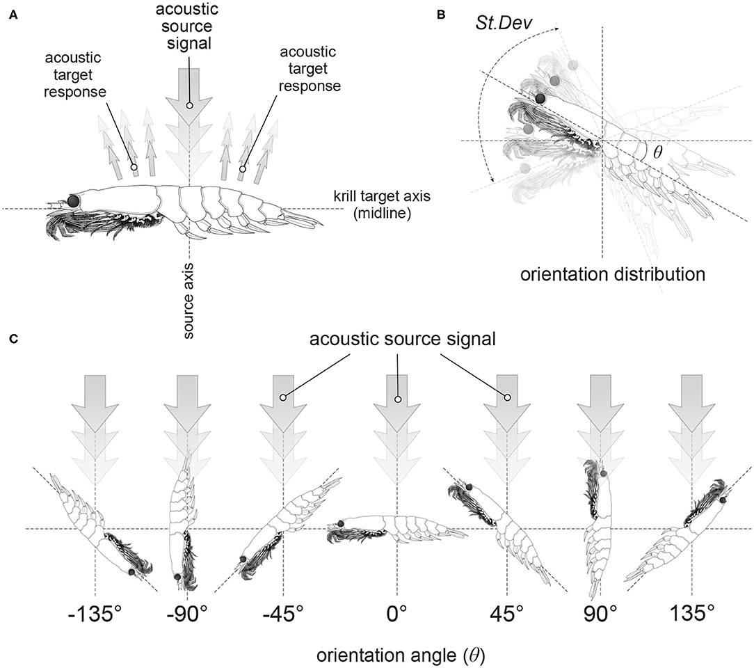
Figure 1. Illustrations of the orientation of krill. Panel (A) shows the orientation of a krill in relation to an acoustic source signal incident perpendicular to the krill midline. This particular orientation is described as broadside incidence. Panel (B) demonstrates an orientation distribution of krill described by a normal distribution with a mean orientation angle, θ and a standard deviation, St.Dev. Examples of krill at discrete orientation angles are displayed in (C).

FIGURE 2

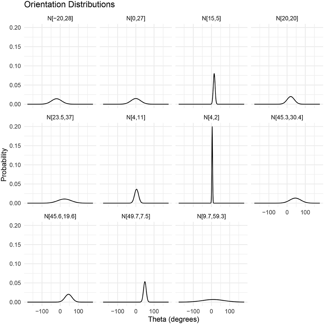
Figure 2. Visualizations of reported normal distributions of krill orientations described by $N[\bar{\theta },St.Dev]$ where $\bar{\theta }$ is mean orientation angle and St.Dev is standard deviation. From left to right, top to bottom: N[−20°, 28°] (CCAMLR, 2010); N[0°, 27°] (Lawson et al., 2006); N[15°, 5°] (Demer and Conti, 2005); N[20°, 20°] (Chu et al., 1993); N[23.5°, 37°] (Letessier et al., 2013); N[4°, 11°] (Conti and Demer, 2006); N[4°, 2°] (Conti and Demer, 2006); N[45.3°, 30.4°] (Kils, 1981); N[45.6°, 19.6°] (Endo, 1993); N[49.7°, 7.5°] (Endo, 1993); N[9.7°, 59.3°] (Lawson et al., 2006).

The combination of both length distributions and orientation distributions is expected to adequately account for the shape variation within a swarm of krill. However, introducing geometric shape, which is normalized in terms of size, position, and orientation, as a variable could improve the accuracy of target strength calculations. While, the orientation distribution may remain a limiting factor in the accuracy of biomass estimates the effect of its uncertainty may be reduced with this method.

1.1. Shape Analysis

Previous work has explored the shape variation of krill both in terms of biology and spatial differences (Finley, 2006; Färber-Lorda et al., 2009; Lorda and Ceccaldi, 2020). Geometric morphometrics is a technique widely used to analyse and compare the geometric shape, i.e., the geometric features and properties remaining when size, position and orientation are excluded or normalized (Zelditch, 2012; Rohlf, 2015). As such, this method provides an alternative to linear measurements, e.g., length, which are entirely dependent on size.

Landmark-based geometric morphometrics sees a biological shape expressed as a series of cartesian coordinates representing the positions of homologous landmarks and pseudo-landmarks (Webster and Sheets, 2010; Cooke and Terhune, 2014). Homologous landmarks are placed at anatomical locations, such as the rostrum on a crustacean, which are identifiable on all specimens of the same species. The use of homologous landmarks allows for repeatable comparison between specimens of similar morphology (Bookstein, 1992; Rohlf and Marcus, 1993). Additional pseudo-landmarks can also be included in areas where homologous landmarks are sparse, to better define the shape. These landmarks are often placed around the outline or at the end of structures (Rohlf and Marcus, 1993). Their positions must be clearly defined to ensure they are comparable across specimen.

Generalized Procrustes Analysis, or superimposition, is used to normalize the landmark coordinates such that the variables of size, position, and orientation are no longer present (Rohlf, 1990). These normalized coordinates are then projected on a linear tangent space for multivariate analyses (Adams et al., 2004). The results can be visualized graphically in terms of the original configurations of landmarks (Adams et al., 2004).

1.2. Scattering Regions

The frequency dependence of target strength is illustrated in Figure 3 for three lengths of krill. The frequency axis is divided into three sections indicating the dominant scattering mechanism. At low frequencies, when the largest dimension of the krill is much smaller than the wavelength of the incident acoustic wave (kL < 1) Rayleigh scattering is the dominant process. In this region the scattering amplitude is proportional to the square of the wavenumber and volume. Here orientation and shape have negligible influence because the whole surface re-radiates an acoustic wave with the same phase.

FIGURE 3

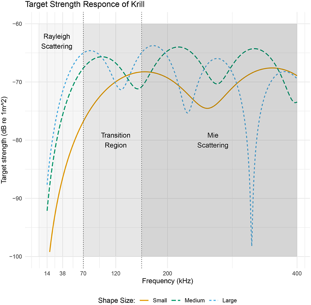
Figure 3. A target strength vs. frequency plot of three sizes of realistic krill shapes with lengths 34.3, 48.6, and 58.9 mm. Target strength data was produced using the DWBA in ZooScatR. The x axis is split into three regions two of which indicate a dominant scattering regime, Rayleigh or Mie, applicable to all three krill. The central portion of the graph highlights the transition between these two scattering mechanisms. The point of transition is taken to be the center of the first turning point (Stanton et al., 1998), which fall at approximately 70, 100, and 160 kHz. Within the Rayleigh scattering region, the target strength does not depend on shape whereas in the Mie scattering region the shape dependence of target strength becomes important resulting in oscillations along the frequency axis.

As the wavelength of the acoustic radiation becomes comparable with the target size there is a transition into the Mie scattering regime. In this frequency region, the phase of the acoustic wave varies both within each cross-sectional slice and along the length of the krill body (Stanton et al., 1998). This complex phase variability gives rise to constructive and destructive interference producing an oscillatory pattern; the period of which depends on krill shape, size, and the instantaneous orientation. Therefore, it is in this frequency region where orientation and shape have the most significant impact on target strength.

At higher frequencies, where krill length is much greater than the wavelength of the incident acoustic wave, the dominant process is geometric scattering. Here the variation in target strength with frequency is greatly reduced. The frequency region, greater than 200 kHz, however, is of less interest in this work as it is often excluded from use in ship-based acoustic surveys due to increased absorption of high frequency sound in sea water (Robertis and Higginbottom, 2007; Macaulay et al., 2020).

1.3. Objectives

The objective of this work is to examine sensitivity of target strength response to Krill shape. A catalog of measured krill shapes is developed and the variability of target strength for these shapes is explored. We also examine the performance/validity of a shape catalog by constructing an equivalent population of a scaled generic shape for comparison. This is accomplished using geometric morphometrics to calculate the average shape of the shape catalog to be used as a scalable generic shape.

2. Materials and Methods

To incorporate shape variation in our model, we have used a catalog of 147 digitized shapes from individually photographed krill collected during a previous study in the East Antarctic (BROKE-West; Nicol et al., 2010). Krill were collected at 50 stations using a Rectangular Mid water Trawl net (RMT-1+8 meter square) (Kawaguchi et al., 2010).

2.1. Krill Shape Digitization

The lateral views of each krill were photographed by a digital camera next to a 1 mm square grid to provide scale. Using the TpsDig v2.04 program (Rohlf, 2005a) from the Tps series of software (Rohlf, 2015), a series of 30 landmarks were manually identified on each image, Figure 4. Of these, 22 landmarks are homologous locations, anatomical points, identifiable on each krill, and 8 are pseudo-landmarks used to define the curve of the krill body where homologous landmarks are widely spaced. The selected landmarks define the outline of the krill, however, during capture, death, and/or preservation, the abdomen of krill specimens tends to curve in an unnatural way, Figure 4. To define a krill shape that better represented a living krill, any curving of the abdomen was statistically removed using the “Unbend specimens” module within the TpsUtil v1.33 program (Rohlf, 2004b). The module works by specifying points along the dorsal side of the krill to which a quadratic curve is fitted so that a transformation may be calculated such that the curve becomes a horizontal straight line. This enabled krill with varying degree of bending in shape to be transformed, hence removing curvature, and standardizing the dorsal landmarks.

FIGURE 4

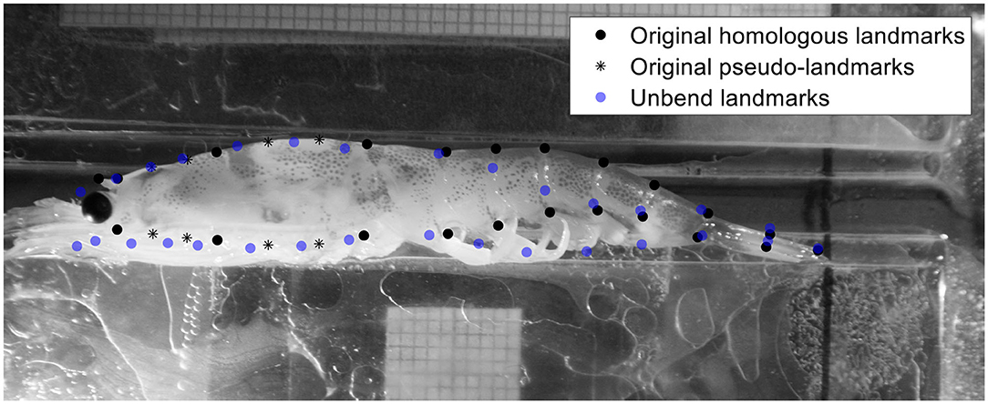
Figure 4. Grayscale image of a krill with superimposed landmark positions. The original landmarks are shown as black markers, 22 of which are placed in homologous locations on the krill and a further 8 pseudo-landmarks, star shaped markers, in positions where homologous landmarks are sparse. In blue are the landmarks transformed by the unbend function which removes post-mortem bending to ensure a realistic shape is captured. The graph paper in the image has a 1 mm square scale.

The landmark configurations output by the “Unbend specimens” module were converted into shape profiles, i.e., the form of a shape compatible with the R package ZooScatR (Gastauer et al., 2019). A shape profile is a file containing a series of circular elements that approximates the shape of a krill. An example shape profile is shown in Table 1 where the first two columns define points along a midline and the third column gives values of cylinder radius at each of these midline points. Each shape profile was produced by considering the landmarks of each krill as two sets, those on the dorsal side and those on the ventral side. Cubic spline interpolation was used calculate corresponding coordinates from the two sets which when subtracted give the midline of the krill. Radius values were then calculated by subtracting the midline from the dorsal line.

TABLE 1

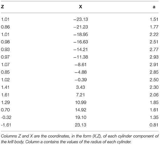
Table 1. A table describing the shape profile of the average shape compatible with ZooScatR.

2.2. Average Krill Shape

An average krill shape was produced using geometric morphometric analysis of the 147 individual krill shapes, employing the Tps series of software (Rohlf, 2015) including: TpsUtil v1.33 (Rohlf, 2004b), TpsDig v2.04 (Rohlf, 2005a), TpsRelw v1.42 (Rohlf, 2005b), Tps Regr. v1.30 (Rohlf, 2004a). A detailed explanation of the method can be found in Rohlf (1990). This process required the landmarks of the individual shapes to be normalized in terms of position, orientation, and scale, mathematically removing all “non-shape” variation. The average krill shape, described as the consensus shape within the Tps software, can be understood as a principal components analysis; effectively independent of size and defined based on the ratio of length to radius.

2.3. Target Strength Model

Krill target strength was calculated using the DWBA approach implemented in the R package ZooScatR v 0.4 (Gastauer et al., 2019). Within ZooScatR the parameterization of the DWBA model is divided into four categories: shape, orientation, material properties, and simulation parameters. The variables within each of these categories were set within a configurations file, Table 2. ZooScatR incorporates a scaling functionality where any shape profile input is first normalized and then scaled depending on the specified length and ratio of length to radius within the configurations file. This allows for easy scaling of a shape to dimensions other than those of the initial shape profile. Therefore, by manipulation of the variables length and ratio of length to radius, we can investigate the effects of size while shape remains unperturbed.

TABLE 2

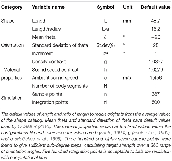
Table 2. A table of parameters, and their default values, contained in the configurations file used in ZooScatR.

3. Results

3.1. Shape Catalog

Landmarks configurations were produced for 147 photographed krill, which were then converted into individual shape profiles compatible with ZooScatR. Figure 5 displays the distribution of krill sizes in terms of the linear measurements of length, L, and ratio of length to maximum radius, L/a. The average length is 48.7 mm with a standard deviation of 4.1 mm. The average ratio of length to radius is 16.2 with a standard deviation of 1.6. The average krill shape, calculated from the 147 individual shapes using geometric morphometrics, takes these average values as its length and ratio of length to radius. This catalog of krill shapes illustrates the diversity of realistic krill body shapes; however it is not assumed to be necessarily representative of the full range of body shapes possible.

FIGURE 5

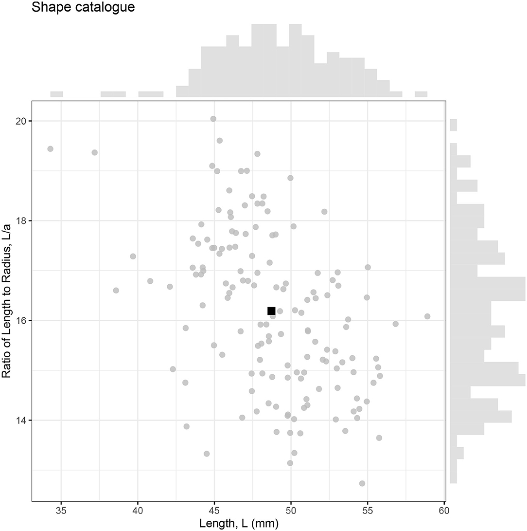
Figure 5. The relationship between krill length (L) and ratio of length to maximum radius (L/a) for 147 krill samples. Each krill is represented by an individual point with the average shown as a black square. Marginal histograms display the distributions of length and ratio of length to radius within the catalog.

3.2. Shapes Influence on Target Strength

The effect of shape on target strength was investigated using the catalog of krill shapes with fixed values of length and ratio of length to radius. This results in a range of target strengths that are a reflection of variation in geometric shapes, independent of length and ratio of length to radius, Figure 6.

FIGURE 6

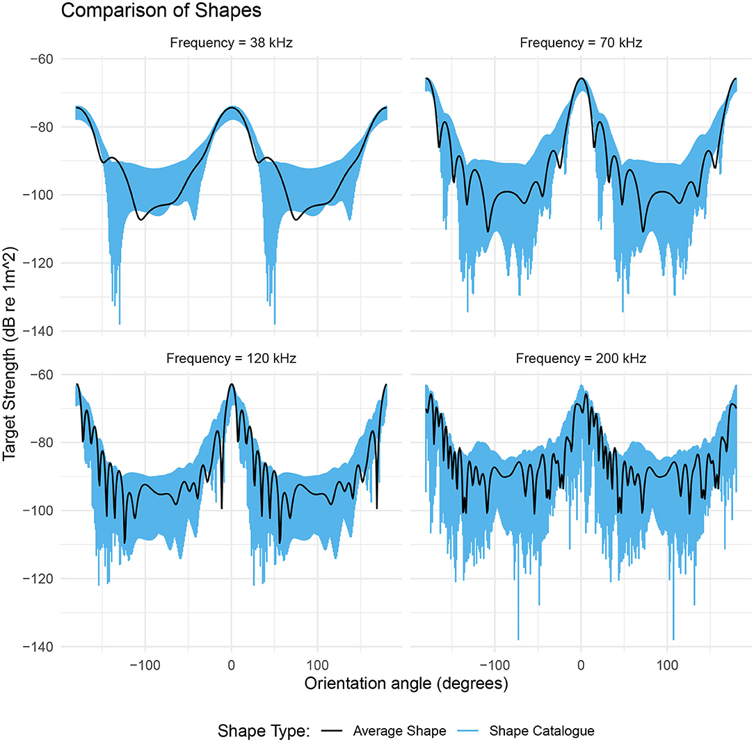
Figure 6. The range of target strengths given by a catalog of shapes scaled to a length of 48.7 mm and a ratio of length to radius of 16.2 (blue region). The black line is the target strength of the average shape with these same dimensions. The target strength of the average shape (black line) generally falls within the range of values produced by the shape catalog (blue region). The target strength response of the shape catalog highlights the orientation dependence of the dominant scattering mechanism. For acoustic frequencies below 200 kHz, the range of target strengths is at a minimum at θ ≈ 0° and at a maximum at θ ≈ 90°.

At the lower frequencies 38, 70, and 120 kHz, the target strength responses of the shape catalog are dependent on orientation, Figure 6. At 70 kHz the target strength responses have a 4 dB range at broadside incidence (θ = 0°). This range increases by over 320% to 13 dB at non-broadside incidence (θ = 90°). At 200 kHz, the catalog of krill shapes produces a variability in target strength across all orientations. The mean range in target strength is 25 dB with a standard deviation of 7 dB.

Target strength of the average shape falls within the range produced by the shape catalog in 87% of cases across all four acoustic frequencies. The general trend in target strength, with orientation angle, is also similar for both the shape catalog and the average shape, Figure 6.

3.3. A Comparison of Shape Populations

We have considered two populations of krill shapes: firstly, a population directly from the shape catalog with measured values of length and ratio of length to radius and secondly, a population consisting of the average shape scaled to each of the combinations of length and ratio of length to radius in the first population. We therefore have two populations with krill ranging in length and ratio of length to radius, however, the geometric shape varies only within the shape catalog population.

Figure 7 illustrates the range of target strength responses for both populations. By scaling the length and ratio of length to radius of the average shape we have introduced variation in target strength. At near broadside incidences, (θ ≈ 0°), the range of target strengths is similar for both populations. For example, at 38 kHz the shape catalog produces target strength responses covering a 16 dB range, centered at −79 dB compared to an 18 dB range centered at −77 dB produced by the average shape population. However, this apparently small, 2 dB change in the target strength translates to a 1.6 times increase of the absolute backscatter in linear terms when using the average shapes compared to the shape catalog.

FIGURE 7

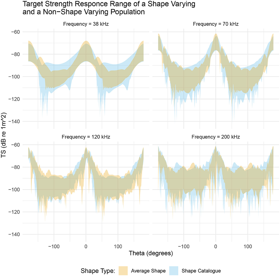
Figure 7. A comparison between a shape varying population, produced from the shape catalog (blue region), and a non-shape varying population, produced by scaling the average shape (orange region). Both populations occupy a similar target strength region however the shape catalog (blue region) typically produced a greater range of target strength responses. This is particularly evident at 38 kHz.

At low frequencies, 38 and 70 kHz, the range of target strength response at non-broadside incidences (θ ≈ 90°) varies between the two populations. At 38 kHz the shape catalog produces a 22 dB range of target strength responses, centered at −100 dB, compared to a 14 dB range centered at −102 dB produced by the average shape population. In linear terms this is a 6.3 times increase of the absolute backscatter.

3.4. Shape, Length and Orientation Distribution

Figures 6 and 7 illustrate the considerable variation in target strength with orientation angle, independent of shape. Therefore, in Figure 8, we have considered weighting using 11 previously reported orientation distributions: N[−20°, 28°] (CCAMLR, 2010); N[0°, 27°] (Lawson et al., 2006); N[15°, 5°] (Demer and Conti, 2005); N[20°, 20°] Chu et al. (1993); N[23.5°, 37°] (Letessier et al., 2013); N[4°, 11°] (Conti and Demer, 2006); N[4°, 2°] (Conti and Demer, 2006); N[45.3°, 30.4°] (Kils, 1981); N[45.6°, 19.6°] (Endo, 1993); N[49.7°, 7.5°] (Endo, 1993); N[9.7°, 59.3°] (Lawson et al., 2006).

FIGURE 8

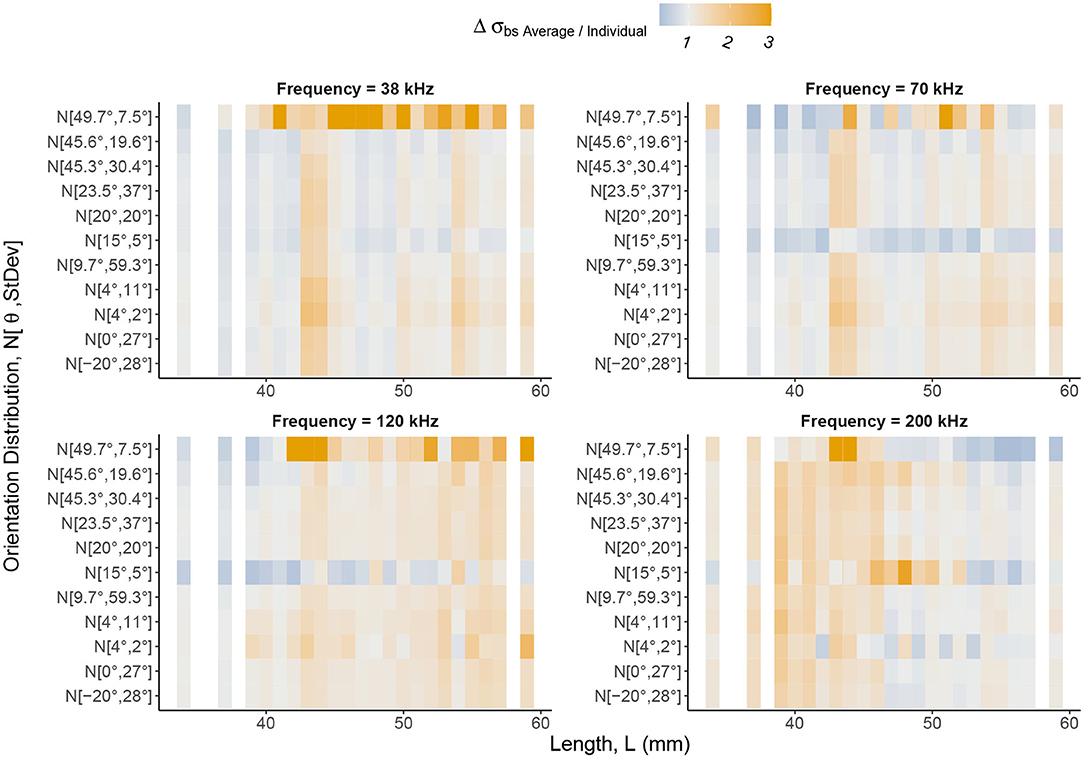
Figure 8. The relative change in backscattering cross-section, Δσ_bs = σ_bsAverage/σ_bsIndividual, between the average and individual, catalog shapes with weighting using orientation distributions applied. Backscattering cross-section can be understood as a linear form of target strength. The Δσ_bs color scale highlights values of Δσ_bs greater than one in shades of orange and values between zero and one in shades of blue. Gray regions are where Δσ_bs is close to one meaning there is little or no change in backscattering cross-section between an average shape and an individual, catalog shape. The notation of the y axis expresses normal distributions of orientation angles in the form $N[\bar{\theta },St.Dev]$ where $\bar{\theta }$ is mean orientation angle and St.Dev is standard deviation. Krill are divided into lengths along the x axis. Distinct vertical bands of Δσ_bs indicate lengths, regardless of orientation distribution weighting, at which Δσ_bs is consistent. Therefore, variation in target strength, introduced by considering geometric shape, is persistent despite averaging using orientation distributions. Δσ_bs is also length dependent, with the region of largest Δσ_bs shifting to lower lengths as frequency increases as a result of transitions between dominant scattering mechanisms.

The change in backscattering cross-section between each cataloged shape and the corresponding scaled average shape was computed for each orientation distribution, Figure 8. This figure reveals vertical bands of similar change in backscattering cross-section across orientation distributions for particular lengths.

At the lower frequencies, 38, 70, and 120 kHz, we see the largest changes in backscattering cross-section at the longer lengths, c. L> 40 mm. For smaller krill, c. L <40 mm, the use of the average shape, typically performs similarly to the shape catalog (gray regions, Figure 8). For example, at 120 kHz, the mean change in backscattering cross-section has increased by a factor of 1.30. This can be interpreted as a 30% increase in backscattering cross-section when using a scaled average shape compared to a shape catalog.

At 200 kHz, the pattern is shifted. The mean change in backscattering cross-section for the shorter krill, c. L < 50 mm. increases by a factor of 1.36 compared to a factor of 1.04 for the longer krill, c. L> 50 mm.

4. Discussion

4.1. Shape and Target Strength

Figure 6 highlights the effect of geometric shape on target strength. The variability in target strength seen across all orientation angles for the individual shapes cannot be reproduced by a generic shape alone.

By comparing target strength response of the shape catalog to an equivalent non-shape varying population, Figure 7, we find that the shape catalog produces a wider range of target strengths. These results suggest that models using a generic shape, scaled with a length distribution, will under-represent the range of target strengths produced by the equivalent individual krill. The scaling of a generic shape is unable to capture the extent of the variability seen for the same population of individual shapes. Furthermore, variation in the change in backscattering cross-section between the average and individual shapes, Figure 8, occurs across all orientation distributions demonstrating that orientation distribution does not mitigate the effect of shape variation. Therefore, despite a potentially unknown orientation distribution, it is reasonable to control for shape variation, using a shape catalog as described above.

4.2. Scattering Mechanisms

We have compared the target strength response of a population of 147 individual krill shapes and an average shape, all scaled to a length of 48.7 mm and a ratio of length to radius of 16.2, Figure 6. At 38 kHz the range of target strength responses varies with orientation angle. This may be understood by noting that the interference of the reflected acoustic wave at near-broadside incidence is dominated by the phase shift along the radius axis of the krill. At non-broadside incidences the dominant scattering mechanism can be determined by the relationship between the length of the krill and the wavelength of the acoustic wave. At low frequencies, the radius is much shorter than the wavelength of the acoustic wave, whereas the length is typically comparable to the wavelength of the acoustic wave. Therefore, as the orientation of the krill varies the dominant scattering mechanism transitions from Rayleigh scattering at near-broadside incidences to Mie scattering at non-broadside incidences. At 200 kHz there is no distinct difference in the range of target strength responses because the wavelength of the acoustic wave is now comparable to both the length and radius dimensions of the krill and Mie scattering dominates for all orientations.

We have also examined the difference in backscattering cross-section of the shape catalog and the equivalent non-shape varying population with various orientation distributions applied, Figure 8. The vertical banding of change in backscattering cross-section for particular lengths can be explained by considering the values of wavenumber, k, length, L, and radius, a. For all four frequencies, kL is greater than 1 indicating that the dominant scattering mechanism is Mie scattering, possibly transitioning to geometric scattering for the longest lengths at 200 kHz. However, ka at 38 kHz, is consistently less than 1 for all shapes so the dominant scattering mechanism, in terms of the radius, is Rayleigh scattering. As the frequency increases ka increases beyond 1 as the dominant scattering mechanism transitions to Mie Scattering.

4.3. Practical Implementation

Determining the length distribution of a krill swarm requires net samples of krill alongside the collection of acoustic data. Therefore, a sample of krill from which shape information can be collected is readily available. The method we have presented uses photographs of individual krill alongside a grid of known scale. These images were collected during a voyage as part of a previous study, demonstrating the ease at which this method can be incorporated into existing protocols.

5. Further Work

The shape catalog we have constructed incorporates 147 krill which were captured from a variety of locations at different times points to ensure a diverse range of shapes. The catalog contains krill shapes with lengths ranging from 34.3 to 58.9 mm. Further work may expand this catalog to give a more extensive view of krill shape diversity over an extended length range. The catalog could also be modified to include fine-scale population dynamics, such as length, sex and stage with which shape is known to vary (Finley, 2006).

The modeled target strength of krill directly impacts biomass estimates. This work could form the basis for new biomass estimates, where shape is incorporated as a variable in target strength calculations.

6. Conclusion

The work presented here is a step toward improving the accuracy of Antarctic krill biomass estimates through the use of a shape catalog. We have focused on modeling the target strength response of both a shape varying and a non-shape varying krill population, at common survey frequencies. Shape was found to have an orientation dependent effect on target strength consistent with the transition between Rayleigh and Mie dominant scattering regimes. The application of a range of orientation distributions does not minimize this effect.

As any biomass estimate for a population of krill is proportional to the backscattering cross section shown in Figure 8, we expect that the use of a shape catalog will result in shifts any such estimates. Therefore, we conclude that it is important to consider the effects of shape as a factor when calculating krill target strength, on which biomass estimates are based.

Data Availability Statement

The research data (and/or materials) supporting this publication can be accessed at doi: 10.17630/1cb66301-633a-47f1-9e58-e813e4c7561e

Author Contributions

FB, SG, and TE conducted the modeling studies. SK assisted with data collection and sample processing and provided technical advice. LF produced the shape catalog. CB and MC contributed to the conception and design of the study. All authors contributed to the article and approved the submitted version.

Funding

FB was funded by an EPSRC studentship (grant code: EP/R513337/1). SG received financial support from the Gordon and Betty Moore Foundation.

Conflict of Interest

LF was employed by the company Elgin Associates Pty Ltd.

The remaining authors declare that the research was conducted in the absence of any commercial or financial relationships that could be construed as a potential conflict of interest.

References

Adams, D. C., Rohlf, F. J., and Slice, D. E. (2004). Geometric morphometrics: ten years of progress following the ‘revolution'. Italian J. Zool. 71, 5–16. doi: 10.1080/11250000409356545

CrossRef Full Text | Google Scholar

Bookstein, F. L. (1992). Morphometric Tools for Landmark Data. Cambridge: Cambridge University Press. doi: 10.1017/CBO9780511573064

CrossRef Full Text | Google Scholar

Calise, L., and Skaret, G. (2011). Sensitivity investigation of the SDWBA Antarctickrill target strength model to fatness, material contrasts and orientation. CCAMLR Sci. 18, 97–122.

Google Scholar

CCAMLR (2010). Report of the Twenty-Ninth Meeting of the Scientific Committee. CCAMLR.

Chu, D., Foote, K. G., and Stanton, T. K. (1993). Further analysis of target strength measurements of Antarctic krill at 38 and 120 kHz: comparison with deformed cylinder model and inference of orientation distribution. J. Acoust. Soc. Am. 93, 2985–2988. doi: 10.1121/1.405818

CrossRef Full Text | Google Scholar

Chu, D., and Ye, Z. (1999). A phase-compensated distorted wave born approximation representation of the bistatic scattering by weakly scattering objects: application to zooplankton. J. Acoust. Soc. Am. 106, 1732–1743. doi: 10.1121/1.428036

CrossRef Full Text | Google Scholar

Constable, A., and De la Mare, W. (1996). A generalised model for evaluating yield and the long-term status of fish stocks under conditions of uncertainty. CCAMLR Sci. 3, 31–54.

Google Scholar

Conti, S., and Demer, D. (2006). Improved parameterization of the SDWBA for estimating krill target strength. ICES J. Mar. Sci. 63, 928–935. doi: 10.1016/j.icesjms.2006.02.007

CrossRef Full Text | Google Scholar

Cooke, S. B., and Terhune, C. E. (2014). Form, function, and geometric morphometrics. Anatom. Rec. 298, 5–28. doi: 10.1002/ar.23065

CrossRef Full Text | Google Scholar

Demer, D., and Conti, S. (2005). New target-strength model indicates more krill in the southern ocean. ICES J. Mar. Sci. 62, 25–32. doi: 10.1016/j.icesjms.2004.07.027

CrossRef Full Text | Google Scholar

Demer, D. A., and Conti, S. G. (2004). Reconciling theoretical versus empirical target strengths of krill: effects of phase variability on the distorted-wave born approximation. ICES J. Mar. Sci. 61, 157–158. doi: 10.1016/j.icesjms.2003.12.003

CrossRef Full Text | Google Scholar

Endo, Y. (1993). Orientation of Antarctic krill in an aquarium. Nippon Suisan Gakkaishi 59, 465–468. doi: 10.2331/suisan.59.465

CrossRef Full Text | Google Scholar

Färber-Lorda, J., Beier, E., and Mayzaud, P. (2009). Morphological and biochemical differentiation in Antarctic krill. J. Mar. Syst. 78, 525–535. doi: 10.1016/j.jmarsys.2008.12.022

CrossRef Full Text | Google Scholar

Finley, L. A. (2006). The biology of Antarctic krill: investigating the shape of krill using geometric morphometrics (Ph.D. thesis). University of Melbourne, Melbourne, VIC, Australia.

Google Scholar

Foote, K. G. (1990). Speed of sound in Euphausia superba. J. Acoust. Soc. Am. 87, 1405–1408. doi: 10.1121/1.399436

CrossRef Full Text | Google Scholar

Foote, K. G., Everson, I., Watkins, J. L., and Bone, D. G. (1990). Target strengths of Antarctic krill (Euphausia superba) at 38 and 120 kHz. J. Acoust. Soc. Am. 87, 16–24. doi: 10.1121/1.399282

CrossRef Full Text | Google Scholar

Gastauer, S., Chu, D., and Cox, M. J. (2019). ZooScatR—an r package for modelling the scattering properties of weak scattering targets using the distorted wave born approximation. J. Acoust. Soc. Am. 145, EL102–EL108. doi: 10.1121/1.5085655

PubMed Abstract | CrossRef Full Text | Google Scholar

Greene, C. H., Stanton, T. K., Wiebe, P. H., and McClatchie, S. (1991). Acoustic estimates of Antarctic krill. Nature 349, 110–110. doi: 10.1038/349110a0

CrossRef Full Text | Google Scholar

Greenlaw, C. F. (1979). Acoustical estimation of zooplankton populations. Limnol. Oceanogr. 24, 226–242. doi: 10.4319/lo.1979.24.2.0226

CrossRef Full Text | Google Scholar

Hewitt, R. P., and Demer, D. A. (2000). The use of acoustic sampling to estimate the dispersion and abundance of euphausiids, with an emphasis on Antarctic krill, Euphausia superba. Fisher. Res. 47, 215–229. doi: 10.1016/S0165-7836(00)00171-5

CrossRef Full Text | Google Scholar

Ikeda, T., and Dixon, P. (1982a). Body shrinkage as a possible over-wintering mechanism of the Antarctic krill, Euphausia superba dana. J. Exp. Mar. Biol. Ecol. 62, 143–151. doi: 10.1016/0022-0981(82)90088-0

CrossRef Full Text | Google Scholar

Ikeda, T., and Dixon, P. (1982b). Observations on moulting in Antarctic krill (Euphausia superba dana). Mar. Freshw. Res. 33:71. doi: 10.1071/MF9820071

CrossRef Full Text | Google Scholar

Kawaguchi, S., and Nicol, S. (2020). “ Krill fishery,” in Fisheries and Aquaculture, eds G. Lovrich and M. Thiel (Oxford: Oxford University Press), 137–158.

Google Scholar

Kawaguchi, S., Nicol, S., Virtue, P., Davenport, S. R., Casper, R., Swadling, K. M., et al. (2010). Krill demography and large-scale distribution in the western indian ocean sector of the southern ocean (CCAMLR division 58.4.2) in austral summer of 2006. Deep Sea Res. II Top. Stud. Oceanogr. 57, 934–947. doi: 10.1016/j.dsr2.2008.06.014

CrossRef Full Text | Google Scholar

Kils, U. (1981). Swimming Behaviour, Swimming Performance and Energy Balance of Antarctic Krill Euphausia superba. Cambridge: SCAR and SCOR, Scott Polar Research Institute.

Google Scholar

Kubilius, R., Ona, E., and Calise, L. (2015). Measuring in situ krill tilt orientation by stereo photogrammetry: examples for Euphausia superbaand meganyctiphanes norvegica. ICES J. Mar. Sci. 72, 2494–2505. doi: 10.1093/icesjms/fsv077

CrossRef Full Text | Google Scholar

Lawson, G. L., Wiebe, P. H., Ashjian, C. J., Chu, D., and Stanton, T. K. (2006). Improved parametrization of Antarctic krill target strength models. J. Acoust. Soc. Am. 119, 232–242. doi: 10.1121/1.2141229

CrossRef Full Text | Google Scholar

Letessier, T. B., Kawaguchi, S., King, R., Meeuwig, J. J., Harcourt, R., and Cox, M. J. (2013). A robust and economical underwater stereo video system to observe Antarctic krill (Euphausia superba). Open J. Mar. Sci. 03, 148–153. doi: 10.4236/ojms.2013.33016

CrossRef Full Text | Google Scholar

Lorda, J. F., and Ceccaldi, H. J. (2020). Relationship of morphometrics, total carotenoids, and total lipids with activity and sexual and spatial features in Euphausia superba. Sci. Rep. 10, 1–15. doi: 10.1038/s41598-020-69780-8

PubMed Abstract | CrossRef Full Text | Google Scholar

Macaulay, G. J., Chu, D., and Ona, E. (2020). Field measurements of acoustic absorption in seawater from 38 to 360 kHz. J. Acoust. Soc. Am. 148, 100–107. doi: 10.1121/10.0001498

PubMed Abstract | CrossRef Full Text | Google Scholar

MacLennan, D. N., Fernandes, P. G., and Dalen, J. (2002). A consistent approach to definitions and symbols in fisheries acoustics. ICES J. Mar. Sci. 59, 365–369. doi: 10.1006/jmsc.2001.1158

CrossRef Full Text | Google Scholar

Mauchline, J., and Fisher, L. R. (1969). “The biology of euphausiids,” in Advances in Marine Biology, eds F. S. Russell and M. Yonge (London; New York, NY: Elsevier), 5. doi: 10.1016/S0065-2881(08)60468-X

CrossRef Full Text

McGehee, D., O'Driscoll, R. L., and Traykovski, L. M. (1998). Effects of orientation on acoustic scattering from Antarctic krill at 120 khz. Deep Sea Res. II Top. Stud. Oceanogr. 45, 1273–1294. doi: 10.1016/S0967-0645(98)00036-8

CrossRef Full Text | Google Scholar

Melvin, J. E., Kawaguchi, S., King, R., and Swadling, K. M. (2018). The carapace matters: refinement of the instantaneous growth rate method for Antarctic krill Euphausia superba dana, 1850 (Euphausiacea). J. Crustacean Biol. 38, 689–696. doi: 10.1093/jcbiol/ruy069

CrossRef Full Text | Google Scholar

Nicol, S., Meiners, K., and Raymond, B. (2010). BROKE-west, a large ecosystem survey of the south west Indian Ocean sector of the Southern Ocean, 30°e-80°e (CCAMLR division 58.4.2). Deep Sea Res. II Top. Stud. Oceanogr. 57, 693–700. doi: 10.1016/j.dsr2.2009.11.002

CrossRef Full Text | Google Scholar

Punchihewa, N., and Krishnarajah, S. (2013). Trophic position of two mysid species (crustacea: Mysidacea) in an estuarine ecosystem in Auckland, New Zealand, using stable isotopic analysis. Am. J. Mar. Sci. 1, 22–27. doi: 10.12691/marine-1-1-4

CrossRef Full Text | Google Scholar

Robertis, A. D., and Higginbottom, I. (2007). A post-processing technique to estimate the signal-to-noise ratio and remove echosounder background noise. ICES J. Mar. Sci. 64, 1282–1291. doi: 10.1093/icesjms/fsm112

CrossRef Full Text | Google Scholar

Rohlf, F. (1990). Proceedings of the Michigan Morphometrics Workshop (Ann Arbor, MI: University of Michigan Museum of Zoology).

Google Scholar

Rohlf, F. (2015). The Tps series of software. Hystrix Italian J. Mammal. 26, 9–12. doi: 10.4404/hystrix-26.1-11264

CrossRef Full Text | Google Scholar

Rohlf, F. J. (2004a). Tps Regr. v 1.30. Department of Ecology and Evolution, University of New York, Stony Brook, New York, NY.

Rohlf, F. J. (2004b). TpsUtil v1.33. Department of Ecology and Evolution, University ofNew York, Stony Brook, New York, NY.

Rohlf, F. J. (2005a). TpsDig v2.04. Department of Ecology and Evolution, State Universityof New York, Stony Brook, New York, NY.

Rohlf, F. J. (2005b). TpsRelw v1.42. Department of Ecology and Evolution, University ofNew York, Stony Brook, New York, NY.

Rohlf, F. J., and Marcus, L. F. (1993). A revolution morphometrics. Trends Ecol. Evol. 8, 129–132. doi: 10.1016/0169-5347(93)90024-J

CrossRef Full Text | Google Scholar

Stanton, T. (2000). Review and recommendations for the modelling of acoustic scattering by fluid-like elongated zooplankton: euphausiids and copepods. ICES J. Mar. Sci. 57, 793–807. doi: 10.1006/jmsc.1999.0517

CrossRef Full Text | Google Scholar

Stanton, T. K. (1989). Sound scattering by cylinders of finite length. III. Deformed cylinders. J. Acoust. Soc. Am. 86, 691–705. doi: 10.1121/1.398193

CrossRef Full Text | Google Scholar

Stanton, T. K., Chu, D., Wiebe, P. H., and Clay, C. S. (1993). Average echoes from randomly oriented random-length finite cylinders: zooplankton models. J. Acoust. Soc. Am. 94, 3463–3472. doi: 10.1121/1.407200

CrossRef Full Text | Google Scholar

Stanton, T. K., Chu, D., Wiebe, P. H., Eastwood, R. L., and Warren, J. D. (2000). Acoustic scattering by benthic and planktonic shelled animals. J. Acoust. Soc. Am. 108, 535–550. doi: 10.1121/1.429584

PubMed Abstract | CrossRef Full Text | Google Scholar

Stanton, T. K., Wiebe, P. H., and Chu, D. (1998). Differences between sound scattering by weakly scattering spheres and finite-length cylinders with applications to sound scattering by zooplankton. J. Acoust. Soc. Am. 103, 254–264. doi: 10.1121/1.421135

PubMed Abstract | CrossRef Full Text | Google Scholar

Webster, M., and Sheets, H. D. (2010). A practical introduction to landmark-based geometric morphometrics. Paleontol. Soc. Pap. 16, 163–188. doi: 10.1017/S1089332600001868

CrossRef Full Text

Zelditch, M. (2012). Geometric Morphometrics for Biologists: A Primer. Amsterdam; Boston, MA: Elsevier Academic Press.

Google Scholar