Improved Calibration and Data Processing Procedures of OPUS Optical Sensor for High-Resolution in situ Monitoring of Nitrate in Seawater

Introduction

Nitrogen is a crucial nutrient for the functioning of all living organisms. The principal form of fixed dissolved inorganic nitrogen in marine waters is nitrate (NO₃^–), which is identified as one of the Essential Ocean Variables by the Global Ocean Observing System community (IOCCP, 2017). Nitrate is used by microorganisms, including phytoplankton, for primary production and thereby facilitates ocean uptake of atmospheric carbon dioxide (Wong et al., 2002). The availability of nitrate leads to direct and indirect effects on marine ecosystem health: it can limit primary productivity when depleted (Kristiansen et al., 2001) and cause eutrophication when supplied at high levels (van Beusekom, 2018). Traditionally, the determination of nitrate in marine waters has been undertaken through collection of discrete water samples, preservation if required, and laboratory analysis using wet-chemical techniques (Grasshoff et al., 1983; Becker et al., 2020). Infrequent sampling intervals result in missing episodic and transient events that lead to important temporal and spatial variations in nitrate concentrations (Prien, 2007; Pidcock et al., 2010). High-frequency in situ observations on autonomous platforms are therefore required to capture the variability in nitrate concentrations, overcome risks of sample contamination and degradation, and reduce high sampling/analysis costs as well as relatively long analysis times.

Over the past 30 years, advances in technology and analytical chemistry have allowed the development of submersible analyzers for marine waters that can provide in situ NO₃^– measurements. To date, wet-chemical colorimetric analyzers and ultraviolet (UV) optical sensor technologies are available for marine water applications (Daniel et al., 2020). These sensors allow autonomous NO₃^– analysis in marine waters on various platforms and at enhanced temporal and spatial resolution. However, their performance can be limited by analytical, biological, optical, and physical factors, including detection limit, reagent stability, biofouling, power consumption, and depth range. Wet-chemical analyzers such as the WIZ probe (Systea, Italy; Vuillemin and Sanfilippo, 2010) and Lab-on-Chip sensor (NOC, United Kingdom; Beaton et al., 2012) have a measurement frequency of ca. 15 min, a limit of detection of 0.025 μM NO₃^–, require chemical reagents, and have moving components (pumps and syringes). The analytical principle is based on the colorimetric reaction method where NO₃^– is determined using the Griess assay with a copperized cadmium column and in situ calibration using standard solutions (Beaton et al., 2012). The optical sensors are based on direct spectrophotometric NO₃^– determinations in the UV wavelength region, as NO₃^– has a strong spectral signature up to 240 nm (Johnson and Coletti, 2002), and these sensors have a high measurement frequency (up to 1 Hz) (Johnson and Coletti, 2002). UV optical sensors offer several advantages over colorimetric sensors, as they are not prone to issues associated with degradation of chemical reagents, fragile microfluidic components, and chemical waste. The optical sensors are small in size (portable), light in weight (typically 2 kg), capable of operating on the order of seconds, and have the potential to be used for long-term deployments because of their low power consumption (≤8 W).

Initial sea trials of the first version of a UV optical NO₃^– sensor measuring at six wavelengths—205, 220, 235, 250, 265, and 280 nm—were reported over 20 years ago (Finch et al., 1998). High-resolution and long-term hyperspectral oceanic measurements of NO₃^– have been reported using a ISUS sensor (Seabird Scientific, United States) that employed a 256-pixel array detector with a spectral range of 200–400 nm (Johnson and Coletti, 2002). Thereafter, various hyperspectral UV optical sensors, such as the SUNA (Seabird Scientific, United States), NITRATAX plus sc (Hach Lange GmbH, Germany), S::CAN Spectro::lyser (S::CAN Messtechnik GmbH, Austria), and ProPS and OPUS (TriOS GmbH, Germany), have become commercially available with a range of detectors, light sources, and path lengths. These sensors have been used in a range of environmental applications, including monitoring of wastewaters (Rieger et al., 2008), freshwaters (Pellerin et al., 2012), coastal waters (Zielinski et al., 2011; Frank et al., 2014), and the open ocean (Johnson, 2010; Pasqueron de Fommervault et al., 2015).

The ISUS sensor has been mounted on autonomous profiling Biogeochemical Argo floats in the ocean, generating high-frequency (1 measurement per second) long-term (>2.5 years) NO₃^– data (Johnson et al., 2013). Recently, the OPUS was deployed in brackish waters of the Baltic Sea in which the potential use of the sensor on a conductivity–temperature–depth (CTD) rosette sampler (1 measurement per 20 s) was demonstrated (Meyer et al., 2018). Bittig et al. (2019) deployed the OPUS on an experimental Biogeochemical Argo float; however to date, results and data evaluations have not been published. The ISUS and OPUS sensors differ in their light sources; ISUS uses a deuterium and OPUS a xenon lamp. Each lamp has a specific thermal and spectral stability, brightness, spectral output, and lifetime (Finch et al., 1998). A xenon flash lamp has a relatively large-scale spectral variability at the wavelength range of interest (<240 nm) compared with deuterium (Johnson and Coletti, 2002), and an advantageously longer lifetime (a xenon lamp ∼2,000–3,000 h and deuterium ∼1,000 h) (Pellerin et al., 2013).

The UV absorption spectrum of seawater is determined by bromide (Br^–) and NO₃^–, and to a lesser extent by the optically measurable fraction of colored dissolved organic matter (CDOM) (Ogura and Hanya, 1966; Johnson and Coletti, 2002). The accuracy of NO₃^– data output using UV optical sensors depends on how well interfering substances are compensated for (Frank et al., 2014). Several data post-processing algorithms have been proposed (Sakamoto et al., 2009, 2017; Frank et al., 2014; Pasqueron de Fommervault et al., 2015; Johnson et al., 2018; Meyer et al., 2018) to correct for the chemical interferences and compute NO₃^– concentrations from raw spectral data. The need to compensate for Br^– interferences in optical nitrate analysis in seawater using temperature and salinity dependence of absorption has been reported (Zielinski et al., 2007). Over 10 years, various oceanographic studies with the ISUS or SUNA sensors commonly used a temperature-corrected salinity subtracted (TCSS) algorithm introduced by Sakamoto et al. (2009, 2017). Calculation strategies of nitrate concentrations from in situ optical nitrate sensors, such as the ProPS, were further improved for turbid marine environments (Zielinski et al., 2011). To date, the OPUS is lacking a reliable sensor calibration and data processing approach for marine waters. There is nevertheless a need to standardize the handling of the raw spectral data of the sensors to ensure the output data is comparable among different studies that cover different regions of the global ocean (Daniel et al., 2020).

The objective of this study was to improve the calibration and data processing procedures of the OPUS for high-resolution in situ monitoring of NO₃^– in marine waters. When handling raw spectral data in different ways, such as using the LSA-like calibration (from the manufacturer, see Table 1) or SUNA-like calibration (Johnson et al., 2018) and distinct approaches to compensate for Br^– and CDOM-related interference in measurements, and comparing the output NO₃^– data might lead to inconsistencies. This study presents a new application of the TCSS approach (introduced by Sakamoto et al., 2009 for the ISUS/SUNA) for the OPUS sensor. For this, sensor-specific parameters related to the calibration and Br^–-compensation algorithm were derived through a series of laboratory experiments. Besides, a total of five OPUS sensors were deployed simultaneously under controlled laboratory conditions, and similarities and differences between the sensors were evaluated. The temporal resolution of NO₃^– measurements by the OPUS sensor has been increased to 3 s by a newly developed controller, achieving high-resolution monitoring on moving marine platforms such as CTD profilers. OPUS sensors were further employed during research expeditions in the (1) southeastern North Sea and (2) tropical Atlantic Ocean. Reference discrete water samples were collected in the field and analyzed in the laboratory using conventional wet-chemical methods for validation purposes.

TABLE 1

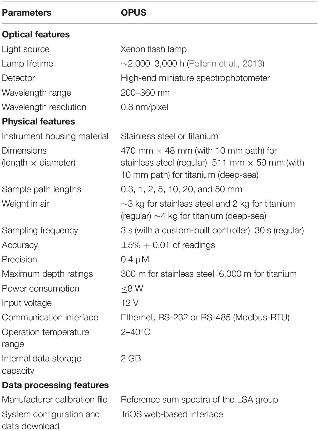
Table 1. Characteristics of the OPUS sensor, as provided by the manufacturer (Operating Instructions, TriOS GmbH, 2017).

Materials and Methods

Instrument Description

The OPUS nitrate sensor is portable, small in size, and light in weight (Table 1). The device uses a xenon flash lamp, a reference diode, and a 256-channel high-end miniature spectrophotometer. Briefly, a xenon flash lamp is directed through an optical path with the sample, and the intensity of light passing through the sample is recorded by the spectrophotometer over a wavelength (λ) range of 200–360 nm with an integration time of 256 ms. A reference diode monitors the intensity of the light source. A schematic diagram of the sensor is shown in Figure 1. All components are housed in a single stainless steel or titanium pressure case.

FIGURE 1

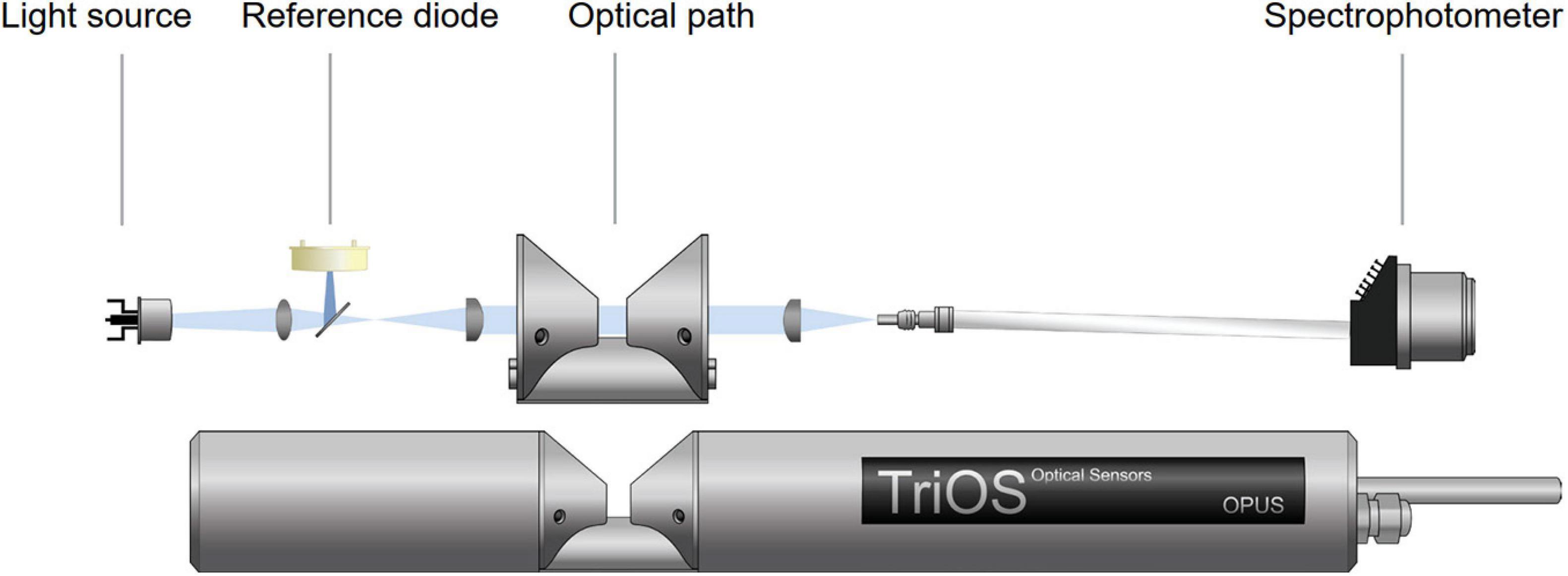
Figure 1. Schematic of the OPUS sensor unit (courtesy of TriOS GmbH, 2017).

The regular (factory setting) sampling interval of the OPUS is 30 s when set to operate in a continuous sampling mode. This is suitable for stationary deployments, but not when deploying the sensor on gliders or autonomous profiler systems, such as CTD frames with a vertical profiling speed of 1 m/s. We developed at GEOMAR an ATMega128 (Atmel Corporation)–based controller that triggers the raw spectral (dark and light) measurements of the OPUS via a Modbus-RTU protocol. The wiring diagram of the controller is provided in Figure 2. Electrical power to the OPUS and controller is provided through an auxiliary port of the CTD system. Measurements are conducted every 3 s at a defined sequence, with measurements of 10 times light followed by one-time dark spectrum. A drift up to 60 s per day in the internal clock of the OPUS was observed. To eliminate this, the controller is set to autonomously synchronize time during each dark measurement. Another important feature of the controller is that it provides backup power for a few seconds to allow the OPUS to finish its measurement in case of power loss.

FIGURE 2

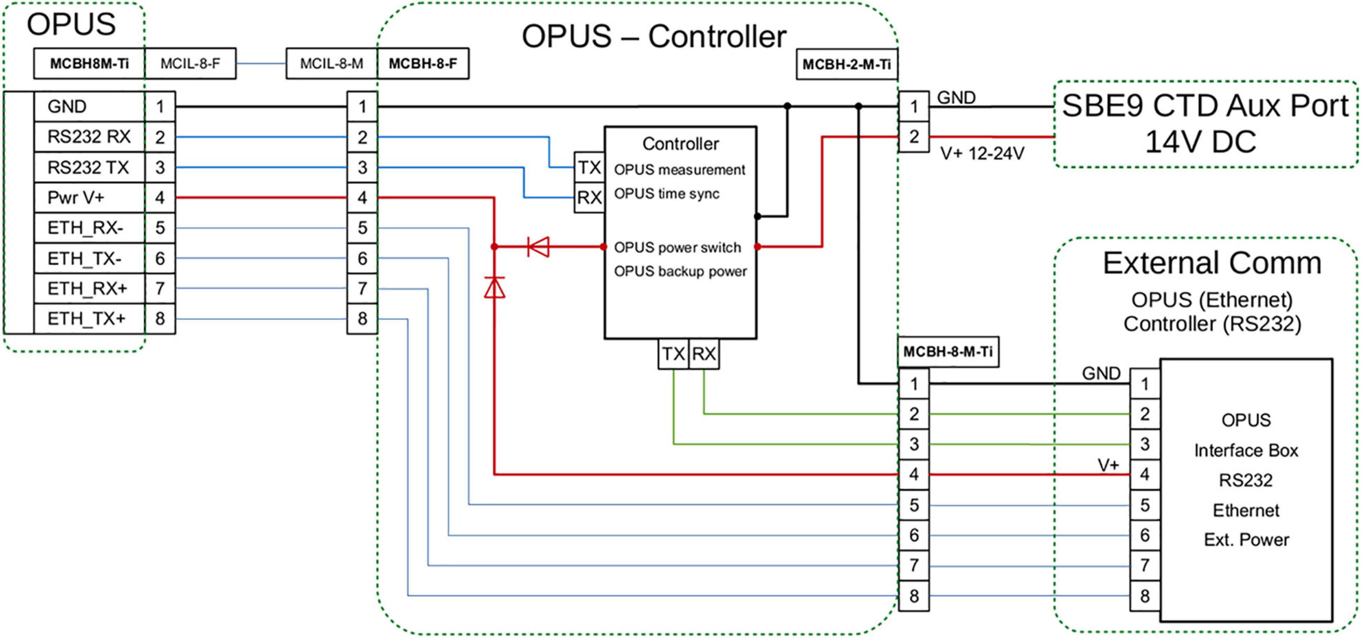
Figure 2. Schematic of the wiring diagram of the controller for enhancing measurement frequency of OPUS sensor.

Laboratory Tests

The first part of this study consisted of experiments carried out under controlled laboratory conditions. Freshly dispensed deionized water (Milli-Q, resistance ≥18 MΩ cm^–1, Merck Millipore) was used to prepare calibration solutions of 840 μM Br^–, with and without 40 μM NO₃^–, and additional 1, 2, 4, 7, 10, 20, and 60 μM NO₃^– solutions, from stock solutions of 1,000 μM KBr (Fisher Scientific ACS reagent grade) and 1,000 μM KNO₃ (Merck Millipore ACS reagent grade). The calibration solutions were kept in acid cleaned (1 M HCl) glass bottles. A total of five OPUS sensors, all with 10 mm optical path length, were used in parallel under conditions described below. We assigned them consecutive numbers, i.e., OPUS1 to OPUS5, to which we refer throughout the study. The OPUS1 sensor was a deep-sea version and others were shallow water versions (see Table 1). The sensors were fully immersed in a thermally insulated glass container (15 L) sequentially filled with calibration solutions in a deionized water medium. The container was connected via Teflon tubing (I.D. 50 mm) to a water bath (7 L, Julabo GmbH) to control the temperature and circulate the solution (Figure 3). A custom-made polystyrene lid was placed on top to avoid contamination and heat exchange, and keep the sensors at the same height in the container. Before the measurements, optical windows of the sensors were cleaned with a few drops of acetone and wipes (Kimtech) followed by rinsing with deionized water. The surface of the sensors, volume of the container, water bath, and tubings contacting sample were all rinsed at least three times with deionized water at the beginning of the setup and between changes of solutions. First, freshly dispensed deionized water was carefully poured into the container, care was taken to avoid the formation of air bubbles on the optical paths, and a reference spectrum was recorded. Then, UV spectra of two calibration solutions were measured as a function of temperature. The water bath temperature was set to a total of four fixed temperatures between 5 and 20°C, and enough time was given to stabilize the sample temperature. The OPUS1 sensor was set to 3 s while the other sensors were set to 30 s for about 30 min (as only one controller for higher frequency analysis was available at the time of the experiment). The calibration solutions were used to assess the temperature effect and to derive molar extinction coefficients—the strength of chemical species to absorb light at a particular wavelength—of Br^– (ε_Br⁻,cal) and NO₃^– (${\mathrm{\epsilon }}_{N{O}_3^{-},cal}$).

FIGURE 3

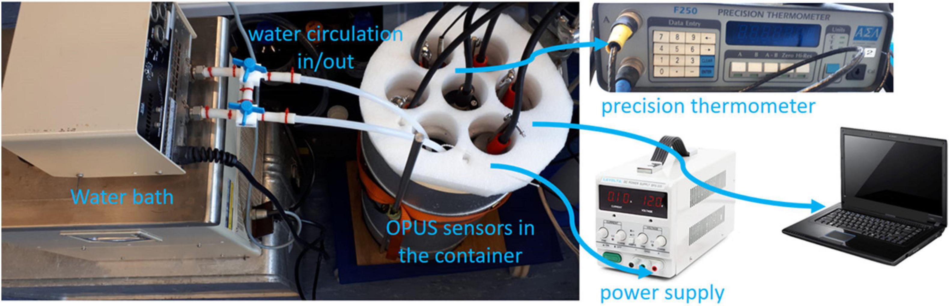
Figure 3. The laboratory setup for testing of OPUS sensors.

Laboratory measurements were conducted in 840 μM Br^–, which is equivalent to Br^– concentrations in seawater with salinity 35. Other chemical interferences from small seawater components are expected to be low below 240 nm, and therefore these were not the subject of this study. The laboratory experiments were conducted in a freshly dispensed deionized water medium to have full control over the measurements and avoid potential matrix effects. The concentration unit of micromolar reported throughout the study indicates micromoles per liter (μmol L^–1).

During the experiments, in situ temperature in the container was measured with a Kelvimat 4323 thermometer (Burster Präzisionsmesstechnik GmbH, 2010) equipped with a Pt100 temperature probe, which has an accuracy of ±0.01°C. The sensors, temperature probe of the precision thermometer, and external computer were all synchronized via coordinated universal time (UTC). The TriOS web-based software was used to operate the sensors and download the internally recorded data. Power (12 V) was supplied to sensors by an external benchtop power supply.

Field Campaigns

One of the OPUS (OPUS1) sensor was employed in the southeastern North Sea on April 16–17, 2019 during the Sternfahrt-1 MOSES research expedition onboard RV Littorina. The expedition track from Büsum to Helgoland and return, and the location of the German Bight are shown in Figure 4. Helgoland is located about 60 km away from the German coast and Elbe River mouth (Ey et al., 2017), and the coastal waters are a mixture of riverine and saline North Sea waters. Before the deployment, the sensor housing was cleaned with deionized water, and the OPUS was fully immersed in a cylinder filled with deionized water to update the water-based spectrum. The sensor was fully immersed in a test tank (volume of 160 L) placed on deck of the vessel and was continuously supplied with surface water (from 2 m depth) at a flow rate of 80 L/min. UV spectral measurements of seawater were recorded with the OPUS at a 1-min sampling interval. In situ salinity and temperature values were recorded at 1-min interval using a CTD system (Seabird SBE 37-SMS-ODO), placed in the test tank. Discrete water samples were collected periodically at about 30-min intervals to validate the sensor measurements. For this, the water samples from the test tank were filtered (0.45 μm pore size PES filter; Fisher Scientific) and stored in 50-ml polypropylene tubes (Jet Biofil) that had been acid cleaned (1 M HCl). The tubes were rinsed three times with filtered seawater before collection. Samples were stored at −20°C and analyzed within 1 month at GEOMAR using an autoanalyzer (Seal QuAAtro) with standard wet-chemical colorimetric techniques (Becker et al., 2020).

FIGURE 4

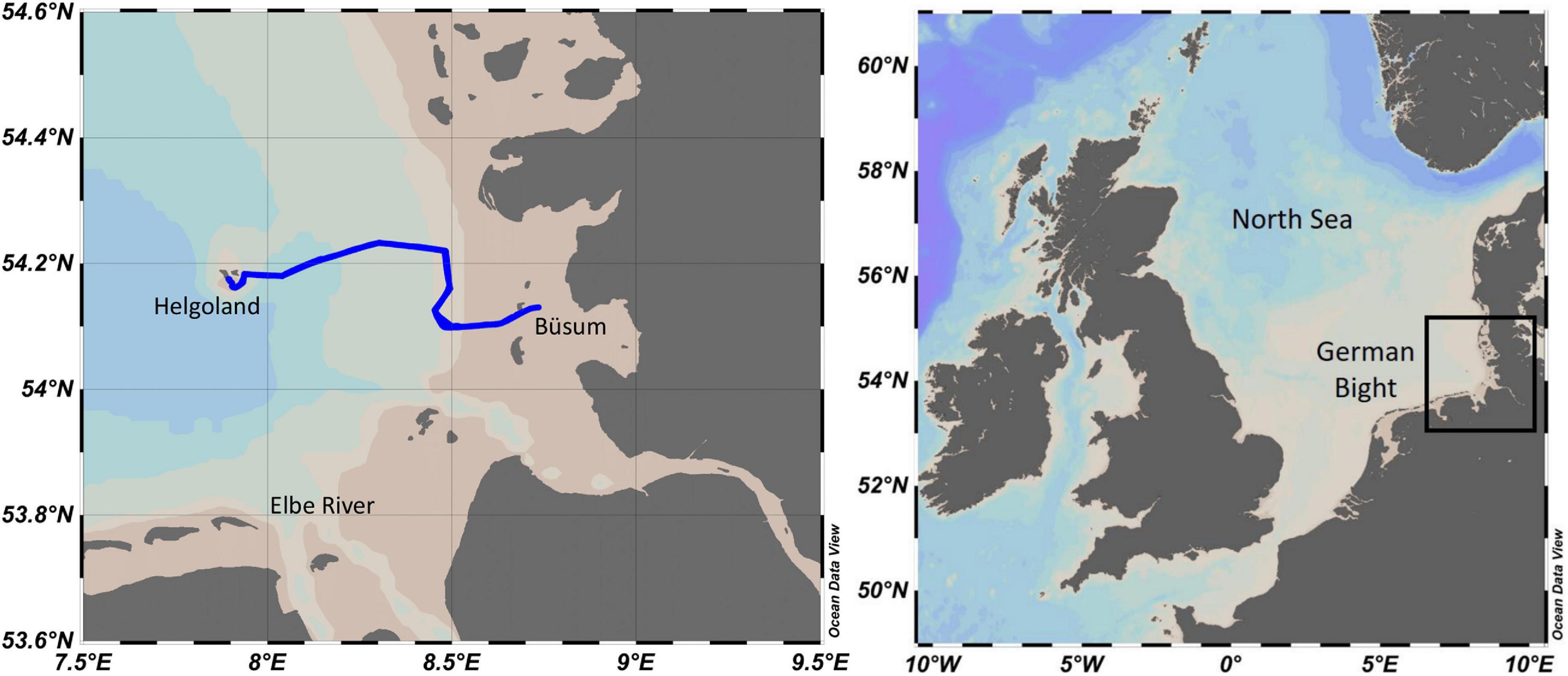
Figure 4. Left panel: map showing the expedition track of the RV Littorina during the Sternfahrt-1 in the southeastern North Sea, from Büsum to Helgoland. Right panel: North Sea and location of the German Bight.

The second field test took place in the tropical Atlantic Ocean, where the OPUS1 was mounted on a CTD frame and deployed on a cast down to 4,000 m depth (00°00.00′S, 30°00.00′W, October 15, 2019, CTD71, M158 research cruise, R/V Meteor). Ancillary data (including dissolved oxygen and inorganic nutrients; NO₃^–, nitrite, silicate, and phosphate) were obtained at various depths during the deployment.

Results and Discussion

Assessment of the Effect of Temperature on Bromide Absorbance

Br^– is a conservative component of seawater with a concentration of ca. 840 μM at salinity 35 (Morris and Riley, 1966). The strength of absorbance for both Br^– and NO₃^– ions are closely related and overlap in the lower UV region, as indicated in a figure of their molar extinction coefficients vs. wavelength (Figure 5). Spectral discrimination of these ions is required to accurately compute NO₃^– concentrations. For this, the spectral region between 217 and 240 nm, where NO₃^– is dominant, is used (Zielinski et al., 2011).

FIGURE 5

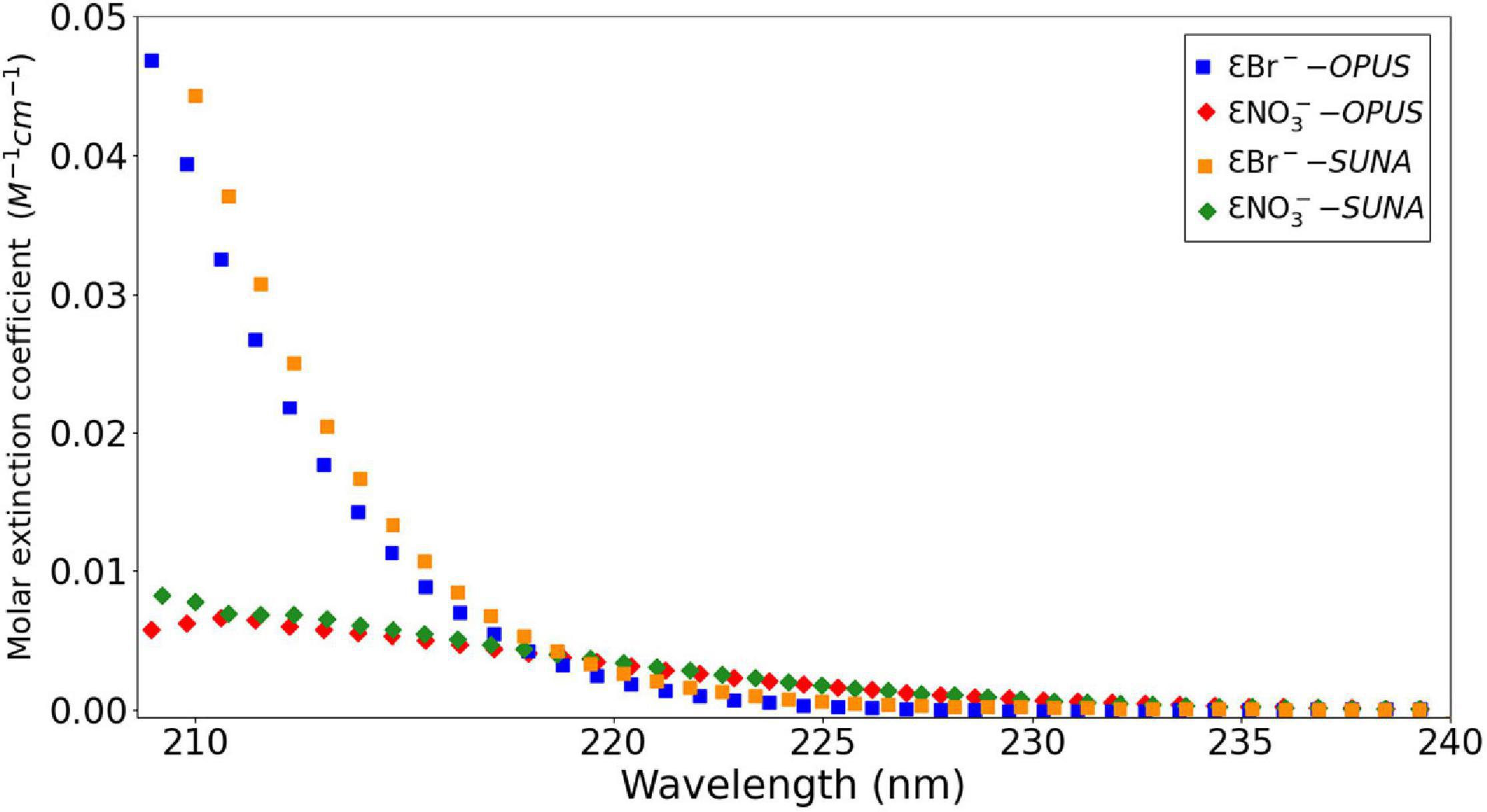
Figure 5. Molar extinction coefficient (ε) values of 840 μM Br^– and 40 μM NO₃^– at wavelengths from 210 to 240 nm at 20°C from OPUS and SUNA-specific (Johnson et al., 2018) calibration files.

Br^– absorption is temperature dependent as it occurs through a charge transfer process; the rate of charge transfer varies with ambient temperature (Jortner et al., 1964; Sakamoto et al., 2009). On the other hand, NO₃^– absorbance is independent of temperature due to the fact that it occurs within the molecule through π to π^∗ transition process (Mack and Bolton, 1999). During the laboratory tests, we used the calibration solutions to assess the temperature effect on Br^– absorbance. The absorbance of the 840 μM Br^– solution exponentially increased with an increasing temperature (Figure 6A), and gradually decreased with increasing wavelength (Figure 6B). The relative change in absorbance with respect to temperature remained constant for 840 μM Br^– with and without 40 μM NO₃^–, there was no additional temperature effect on absorbance due to the presence of NO₃^– ions (not shown here). It should be noted here that the 840 μM Br^– and 40 μM NO₃^– do not necessarily reflect the real seawater conditions, and the exact in situ levels of both constituents might vary in time and space; nevertheless, this can be computed using the algorithm (see Eq. 4 in section “Data Processing Procedure for OPUS”).

FIGURE 6

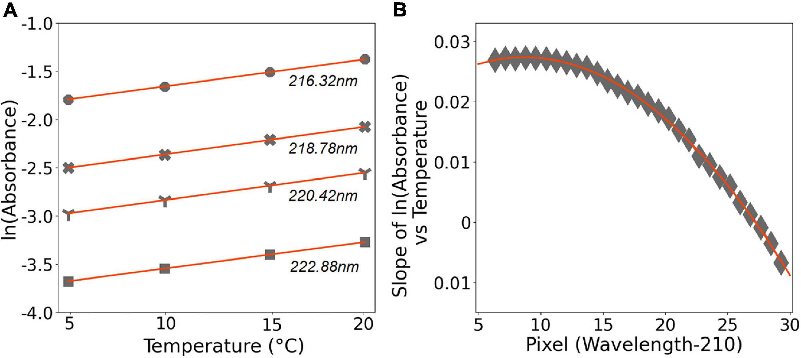
Figure 6. (A) The ln(absorbance) values of 840 μM Br^– solution plotted vs. temperature of the solution; at 216.32, 218.78, 220.42, and 222.88 nm. Data are shown in gray. The solid red lines refer to the linear regression (r² = 0.99), with y = 0.0277x–1.9323, y = 0.0284x–2.6439, y = 0.0282x–3.1159, and y = 0.0271x–3.8135, respectively. (B) The slope of ln(absorbance) vs. temperature plotted vs. pixel. In here, pixel refers to wavelength –210, within 216 and 239 nm. The solid red line presents the third-order polynomial fit and has y = 1e–07x³–9e–05x² + 0.0016x + 0.0212, r² = 0.99.

The raw spectral data of the calibration solutions were processed using the procedure described in section “Data Processing Procedure for OPUS.” An example spectral area attributed to NO₃^– after data processing is shown in Figure 7.

FIGURE 7

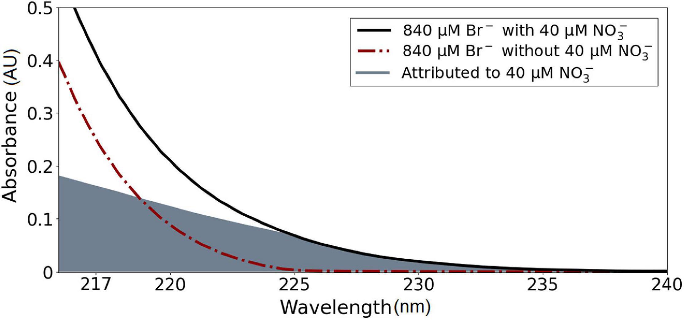
Figure 7. The spectral signature of calibration solutions at 20°C. The gray filled area is attributed to absorbance due to NO₃^–.

Data Processing Procedure for OPUS

Raw spectral data of the OPUS were processed by taking potential lamp degradation, Br^– interference, and CDOM-baseline effect into account before calculating NO₃^– concentrations. The lamp degradation was taken into account during calculation by recording detector intensities in deionized water before and after each deployment (see section “Calibration of OPUS Sensors: Inter-Sensor Comparison”). We determined OPUS-specific molar extinction coefficients for Br^– and NO₃^– before data processing and developed a new algorithm (Eq. 4) for the compensation of Br^– interferences. Data processing procedure is outlined as follows:

1. Calculation of the measured absorbance of a sample in the UV spectral region of interest between 200 and 260 nm: the absorbance (A_measured) is logarithmically related to a transmitted light intensity according to Beer–Lambert’s law:

$$A_{measured}=-\log \left(\frac{I_{\mathrm{\lambda }}-I_D}{I_{\mathrm{\lambda }0}-I_D}\right)(1)$$

where I_λ refers to detector intensity for the sample and $I_{\mathrm{\lambda }}{}_0$ is the detector intensity for deionized water. I_D is the dark current that is periodically recorded by the spectrophotometer when the light source is off. I_D was subtracted from each spectrum to eliminate internal noise (Nehir et al., 2019) before the data are used. λ is the wavelength (nm).

2. Calibration coefficients: it should be noted here that the calibration coefficients were determined in the laboratory following the procedures described in section “Laboratory Tests,” and a sensor-specific calibration file was produced before the deployments. This file includes wavelength, ε_Br⁻,cal, ${\mathrm{\epsilon }}_{N{O}_3^{-},cal}$, calibration temperature, and reference intensity recorded in deionized water (Johnson et al., 2018). ε_Br^–,cal and ${\mathrm{\epsilon }}_{N{O}_3^{-},cal}$ were determined from a linear relationship between absorbance and concentration of the substance according to Beer–Lambert’s Law:

$${\mathrm{\epsilon }}_{B{r}^{-},cal}=\frac{A_{B{r}^{-}cal}}{S_{cal}\cdot l}at{T}_{cal}(2)$$

$${\mathrm{\epsilon }}_{N{O}_3^{-},cal}=\frac{A_{N{O}_3^{-}cal}}{c_{N{O}_3^{-},cal}\cdot l}(3)$$

where A_{Br^– cal} is the absorbance of Br^– calibration solution, and is normalized to a salinity of 35 [for (S_cal = 35 Br^–) = 840 μM]. ${\mathrm{A}}_{N{O}_3^{-},cal}$ is the absorbance of NO₃^– calibration solution, and ${\mathrm{c}}_{N{O}_3^{-},cal}$ is the concentration of the solution, 40 μM. T_cal is the temperature value of the solution during the calibration, 20°C. The units for ε_Br⁻,cal and ${\mathrm{\epsilon }}_{N{O}_3^{-},cal}$ are M^–1 cm^–1, which are dependent on the path length of the sensor. In this study, the optical path length (l) of the OPUS sensors was 10 mm.

3. Br^–-related interference compensation: to compensate Br^– interference in optical nitrate measurements, we determined the relative change in 840 μM Br^– absorbance—salinity normalized to 35—with respect to wavelength and temperature under controlled laboratory conditions. From this, we developed a new algorithm (Eq. 4), based on Figure 6, to calculate Br^– absorbance theoretically at in situ conditions. Previously, it was shown that pressure also has an effect on the Br^– absorbance of about −2% (Pasqueron de Fommervault et al., 2015) or −2.6% per 1,000 dbar (Sakamoto et al., 2017). This correction can be described as follows:

$${\mathrm{\epsilon }}_{Br-,insitu}={\mathrm{\epsilon }}_{Br-,cal}\cdot \exp \begin{array}{c}\hfill (a\cdot w^3+b\cdot w^2+c\cdot w+d\cdot \hfill \\ \hfill (T_{insitu}-T_{cal}))\hfill \end{array}(4)$$

$${\mathrm{\epsilon }}_{Br-,insitu}={\mathrm{\epsilon }}_{Br-,insitu}\cdot (\mathrm{\hspace{0.25em}1}-(P_F\cdot P_{insitu}/1000))(5)$$

$$A_{insituB{r}^{-}}={\mathrm{\epsilon }}_{Br-,insitu}\cdot S_{insitu}(6)$$

$$A_{residual}=A_{measured}-A_{insituB{r}^{-}}(7)$$

where w refers to wavelength minus 210, a wavelength offset (wo) value of 210. It was used for scaling purposes, and is a tunable parameter (Pasqueron de Fommervault et al., 2015; Johnson et al., 2018). ε_Br−,insitu is the molar extinction coefficients of Br^– at the in situ temperature (T_{in situ}, °C), salinity (S_{in situ}) and pressure (P_{in situ}, dbar). The parameters a, b, c, and d are regression parameters of 1e−07, −9e−05, 0.0016, and 0.0212, respectively. The parameters were obtained by fitting the “slope of absorbance of the Br^– calibration solution vs. in situ temperature” to “wavelengths from 216 to 239 nm” (Figure 6) to the third-order polynomial function. P_F refers to a pressure factor of 0.026. A_{in situ Br–} (in situ Br^– absorbance) was then subtracted from A_measured, and A_residual (remaining absorbance) was then used to fit NO₃^– and CDOM. P_{in situ} and S_{in situ} refer to the in situ pressure (dbar) and salinity values, respectively.

Although, in theory, one method for the bromide-temperature relationship (calibration and fit coefficient) should be valid for all sensors, our results demonstrate that in practice the optical differences among each device (lamp, spectrometer, etc.) can have an impact on measurement quality. New fitting (Eq. 4) and calibration coefficients (Figure 5) were introduced for the OPUS sensor, while the overall procedure and handling of the raw spectral data followed the well-developed approaches from the literature.

4. CDOM-baseline correction and NO₃^– quantification: The absorbance due to CDOM, also termed as yellow substances (Frank et al., 2014), often occurs at wavelengths above 240 nm, with a maxima near 260 nm, through electron transition between lone pairs or π-electrons (Guenther et al., 2001; Stedmon and Nelson, 2015). So far, linear (Sakamoto et al., 2009; Zielinski et al., 2011) and quadratic (Johnson and Coletti, 2002) mathematical functions have been proposed for the compensation of this interference, at wavelengths between 240 and 260 nm, based on the shape of the observed absorbance spectra. There appears no obvious difference between a linear and quadratic model, as both approaches are based on rough estimations of CDOM-related absorption spectrum (Frank et al., 2014). The concentrations and characteristics of CDOM are highly variable in natural waters with complex origins. Therefore, the preparation of an artificial solution under laboratory conditions is not ideal to compensate for CDOM interference.

In this study, A_residual was attributed to absorbance due to NO₃^– ($A_{N{O}_3^{-}})$ and CDOM-baseline (A_CDOM). Each spectrum was corrected for the contribution of A_CDOM (Eq. 9), which was determined from the linear regression between absorbance and wavelength (see Figure 8):

$$A_{CDOM}=i+j\cdot \mathrm{\lambda }(8)$$

where i and j refer to baseline intercept and slope, respectively, and are adjustable parameters based on measured in situ absorbance.

The final determination of NO₃^– concentration (${\mathrm{c}}_{N{O}_3^{-},cal}$) was done by solving a linear regression using a singular value decomposition method at approximately 30 pixels (0.8 nm/pixel) within 217 and 240 nm. This can be expressed as

$$A_{residual}=\left[\begin{array}{ccc}1\mathit{\hspace{1em}}\hfill & {\mathrm{\lambda }}_1\mathit{\hspace{1em}}\hfill & {\mathrm{\epsilon }}_{N{O}_3^{-},cal,{\mathrm{\lambda }}_1}\hfill \\ 1\mathit{\hspace{1em}}\hfill & {\mathrm{\lambda }}_2\mathit{\hspace{1em}}\hfill & {\mathrm{\epsilon }}_{N{O}_3^{-},cal,{\mathrm{\lambda }}_2}\hfill \\ & & \mathrm{\dots }\hfill \\ 1\mathit{\hspace{1em}}\hfill & {\mathrm{\lambda }}_{n-1}\mathit{\hspace{1em}}\hfill & {\mathrm{\epsilon }}_{N{O}_3^{-},cal,{\mathrm{\lambda }}_{n-1}}\hfill \\ 1\mathit{\hspace{1em}}\hfill & {\mathrm{\lambda }}_n\mathit{\hspace{1em}}\hfill & {\mathrm{\epsilon }}_{N{O}_3^{-},cal{,}_n}\hfill \end{array}\right]\cdot \left(\begin{array}{c}\hfill i\hfill \\ \hfill j\hfill \\ \hfill c_{N{O}_3^{-}}\hfill \end{array}\right)(9)$$

where λ₁ to λ_n refers to wavelengths between 217 and 240 nm where the Br^– and CDOM interferences are lowest (Sakamoto et al., 2009; Zielinski et al., 2011). ${\mathrm{\epsilon }}_{N{O}_3^{-},cal,}$ is shown in Eq. 3.

Figure 8 illustrates an example of the spectral signature of CDOM on optical NO₃^– determination.

FIGURE 8

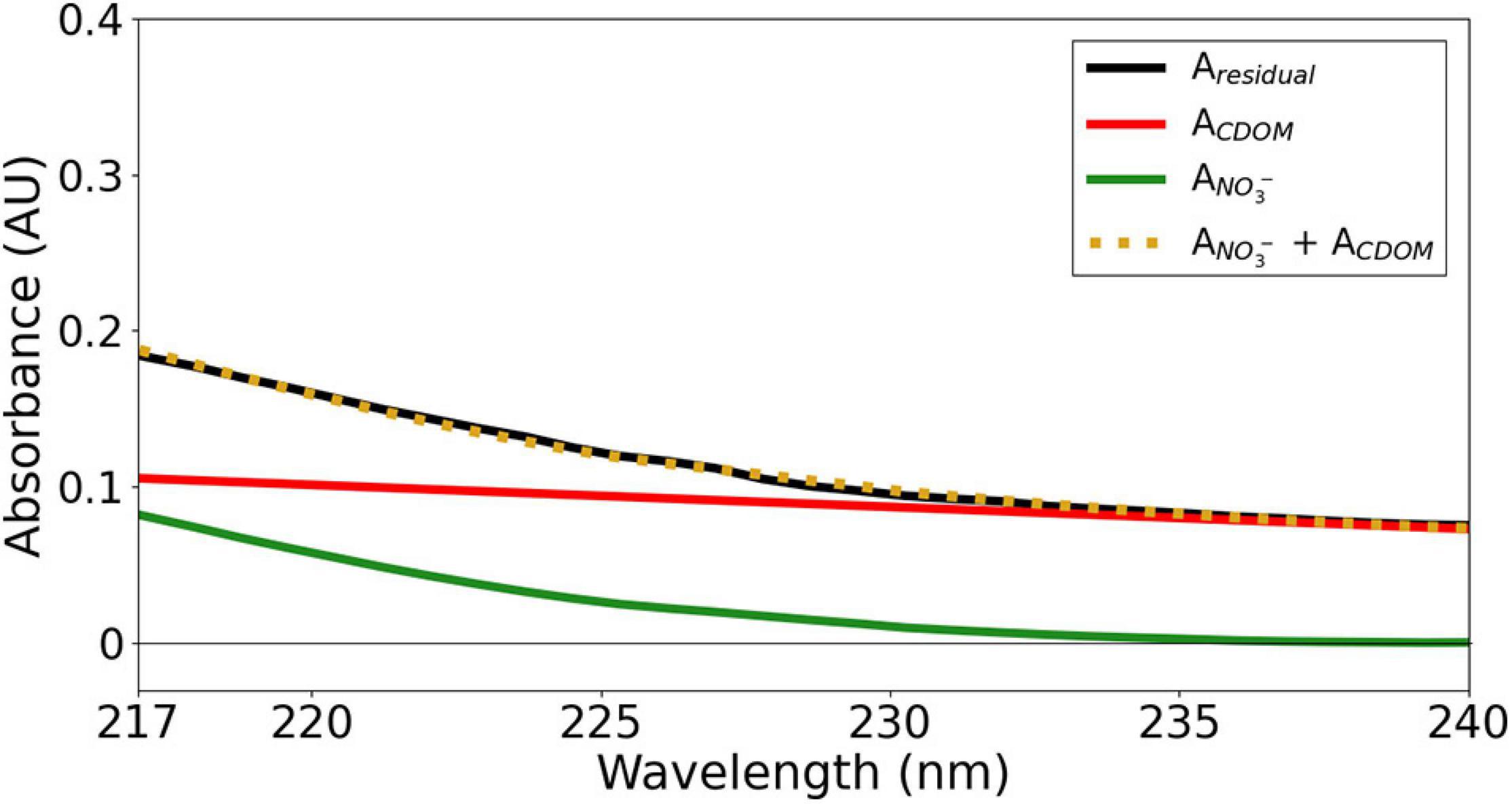
Figure 8. The spectral signature of CDOM and NO₃^– within 217 and 240 nm (cNO₃^– = 19.4 μM, S = 35.4, T = 13.6°C at 211 m depth during the M158-CTD71 deployment).

All data processing described and statistical analysis throughout the study were undertaken in MATLAB (MathWorks, R2018a) software. A mat file with the complete data from each recorded activity was produced. The code ingests the OPUS raw data file, calibration file, CTD file, and all equations above, and is available at https://github.com/uv-nitr/proc.

Calibration of OPUS Sensors: Inter-Sensor Comparison

The OPUS sensor is factory calibrated at the manufacturer and a sum absorption spectra of expected seawater constituents at pre-defined concentrations is saved in the unit (see Table 1, Operating Instructions, TriOS GmbH, 2017). The other optical nitrate sensors, such as the ISUS and SUNA, are calibrated to derive the molar extinction coefficients of Br^– and NO₃^– (Sea-Bird Coastal SUNA, 2015). Recent documentation of these sensors’ calibration and data processing can be found in the “Processing Bio-Argo nitrate concentration at the DAC Level” and “8th BGC-Argo Meeting” reports (Johnson et al., 2018; Claustre and Johnson, 2019). In this work, the factory calibration of the OPUS was ignored and individual calibration coefficients were obtained (Eqs 2 and 3). The correlation for ε_{Br_cal} and ε_{NO3_cal} for about 75 pixels between 200 and 260 nm was examined using the Pearson correlation matrix and coefficients. A correlation coefficient value close to 1.0 indicates an excellent correlation between the respective datasets. Results indicated that the OPUS sensors were in excellent agreement (≥0.95) for both ε_{Br_cal} and ε_{NO3_cal} values (Figure 9), and are greater than 0.99 within 217 and 240 nm (for about 30 pixels, wavelength range of the NO₃^– fit, not shown here). The sensors wavelength values vary about 4–5 nm at the same pixel. Improvement of technical characteristics such as wavelength registrations and gratings in CCDs were beyond the scope of the study. However, the reason for non-identical correlation coefficients for the same pixels can be explained not in absolute value of sensors but in sensitivity. For example, the OPUS1 sensor had a spectral resolution of 0.82 nm while the OPUS2 had 0.79 nm resulting in better sensitivity.

FIGURE 9

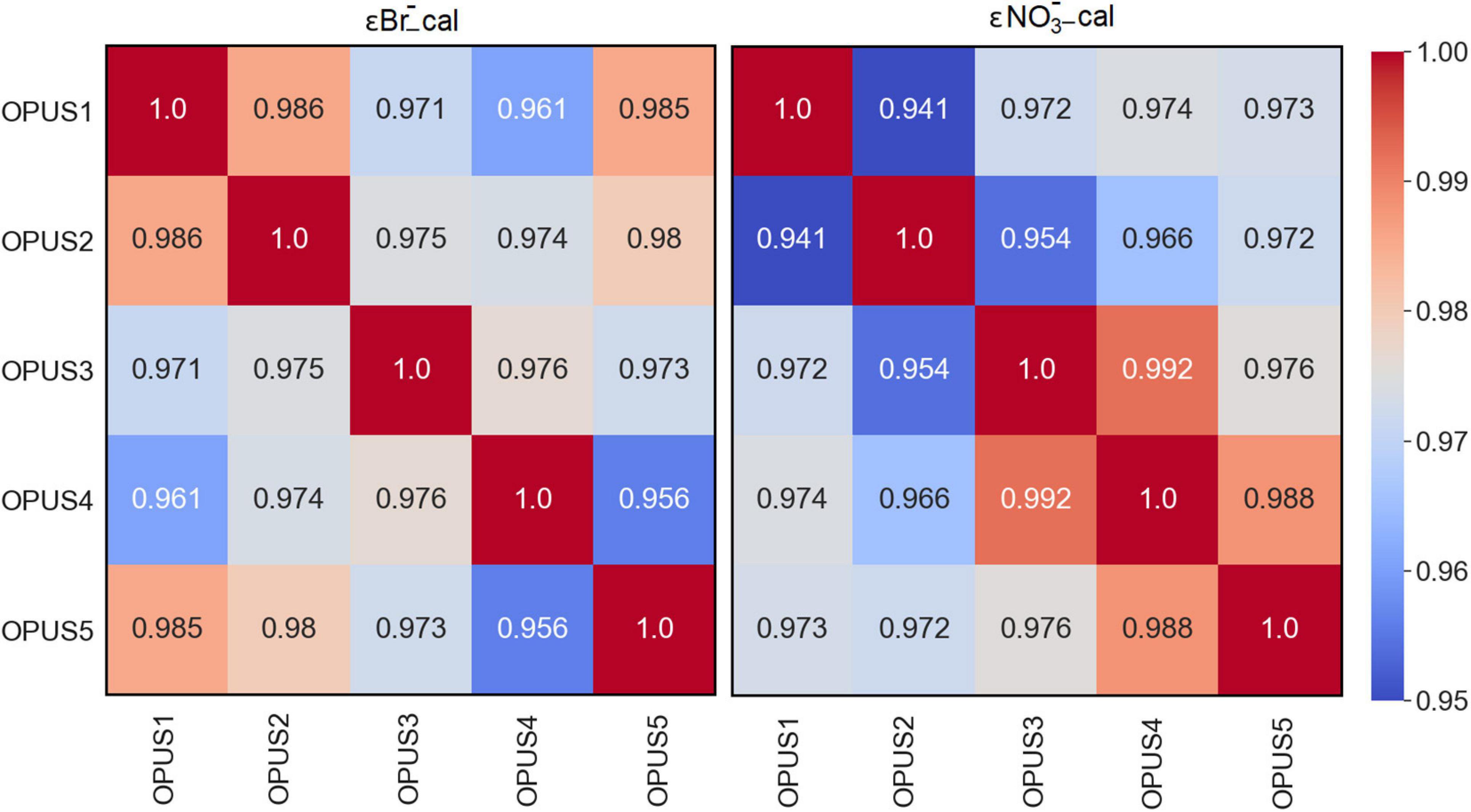
Figure 9. Pearson’s correlation matrix for ε_{Br_cal} and ε_{NO3_cal}for the OPUS sensors used.

Results from the laboratory test of the OPUS sensors under identical conditions, and using a series of 1, 2, 4, 7, 10, 20, 40, and 60 μM NO₃^– solutions in 840 μM Br^– medium, are presented in terms of NO₃^– bias across the five sensors. The NO₃^– concentration obtained from the OPUS sensor with the mean and laboratory analysis of discrete water samples was fit to a linear regression (r² = 0.99; Figure 10). The SD of NO₃^– for the lowest concentration was ∼0.64 μM, which translates to a limit of detection of ca. 2 μM NO₃^– (three times the SD of blank). An accuracy of better than ∼2 μM NO₃^– was determined from the residuals of the regression, while overall precision of NO₃^– sensor measurements was ∼0.4 μM, from the consecutive measurements of the identical sample.

FIGURE 10

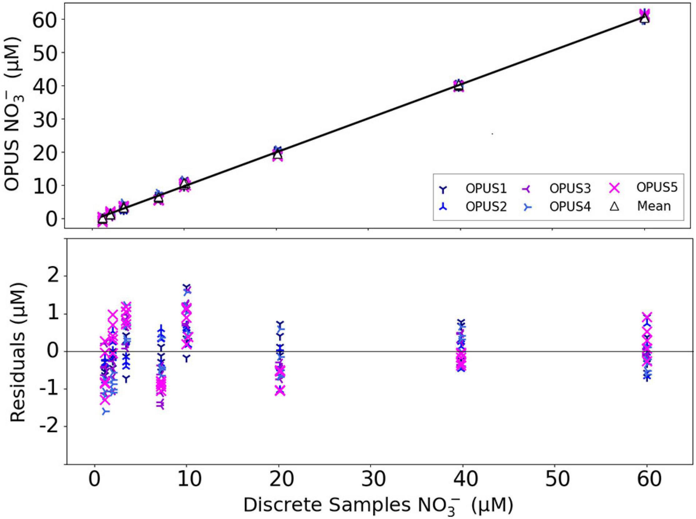
Figure 10. Linear regression fit (solid line) between mean NO₃^– concentrations from the OPUS sensors vs. laboratory analysis of discrete water samples (y = 1.021x–0.641, r² = 0.99). The residuals of the regression for each sensor were within ±2 μM NO₃^–.

An additional parameter used for the calibration is the reference spectrum recorded for deionized water medium using the OPUS sensors. The detector intensity of the sensor in deionized water was used in Eq. 1. Each OPUS sensor has a unique spectral output of its xenon flash lamp in the UV range (Figure 11). The design of the OPUS is comparable with the SUNA, except for the xenon lamp. Although this is not an OPUS vs. SUNA comparison study, a demonstration of reference intensity (recorded in deionized water) values of the xenon lamp–based OPUS sensor and deuterium lamp–based SUNA sensor are shown in Figure 11. Please note here that the data presented for the SUNA sensor were adopted from the literature (Johnson et al., 2018). Observing large differences in spectral output of xenon and deuterium lamps raised concerns regarding the need to derive OPUS-specific coefficients. Therefore, it is important that the true performance of each specific OPUS sensor is verified in the laboratory following well-established guidelines used for other optical nitrate sensors because the varying registrations, resolutions, and flash lamp spectra (i.e., ε values) are specific to each sensor. As this sensor-specific calibration is currently not available from the manufacturer, the five units were compared in the laboratory.

FIGURE 11

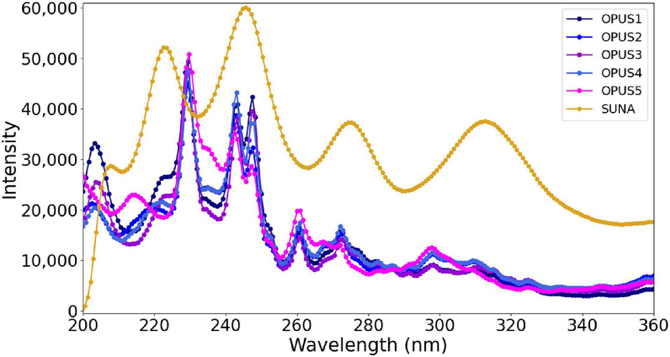
Figure 11. The detector intensity of the optical nitrate sensors in deionized water at all wavelengths.

The five OPUS sensors are not identical in terms of their reference spectrum as each unit has a unique compact spectrometer and wavelength registration. In addition, the sensors are not identical in terms of their age (some were several years old and others several months). The reference spectrum needs to be updated periodically (before and after each deployment) for each individual unit to minimize potential sensor drift due to aging of the lamp or obstacles in the optical path (Pellerin et al., 2013) and ensuring sensor stability over time.

Field Deployments

The second part of this study focused on the validation of the NO₃^– computational algorithm for the OPUS. Real-time in situ measurements were undertaken with the OPUS1 and CTD sensors during the Sternfahrt-1 MOSES expedition in the North Sea, where the influence of the outflow plume of the Elbe River is pronounced (Voynova et al., 2017). Temporal trends in surface water variables such as temperature, salinity, and NO₃^– were determined along the cruise track. The Elbe system is subject to short-term dynamic extreme events such as heatwaves and heavy rainfall which significantly affect the waters of the southern North Sea (Voynova et al., 2017; Chegini et al., 2020). A total of 730 measurements were performed by the OPUS sensor during the 2-day cruise period. The time series of NO₃^–, temperature, and salinity are shown in Figure 12. The NO₃^– values ranged between 24.6 and 70.9 μM on the first day (Figure 12A), and 14.2–60.7 μM on the second day (Figure 12B). Temperature ranged between 7.22 and 8.34°C, and salinity between 24.09 and 31.66.

FIGURE 12

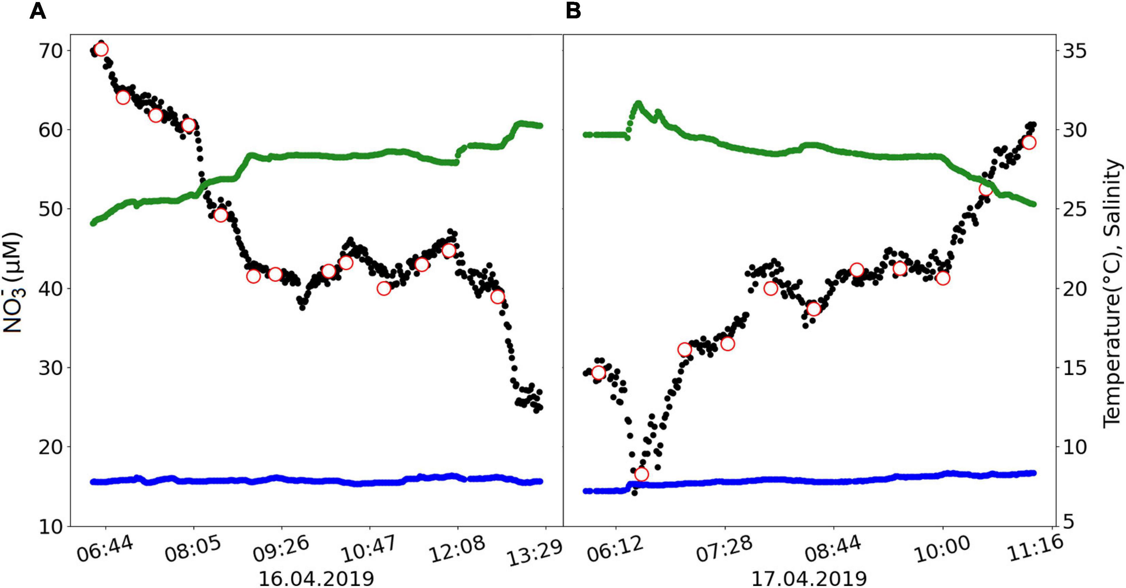
Figure 12. Time series of NO₃^– (μM), temperature (°C), and salinity during the Sternfahrt-1 expedition on (A) the first day sailing from Büsum to Helgoland and (B) the second day sailing from Helgoland to Büsum. Black dots refer to the post-processed OPUS NO₃^– data output, and red circles are the NO₃^– concentrations of the discrete water samples analyzed in the laboratory by a wet-chemical analyzer. Blue and green dots indicate the in situ temperature and salinity of the sample, respectively.

The high variability in NO₃^– concentrations over short time scales during the approximately 6-h transects can be attributed to dynamic interactions between the waters of the North Sea and the Elbe River, with additional mixing through tidal actions. Enhanced salinity levels (toward 32) away from the coast and Elbe River coincided with lower NO₃^– concentrations (14.2 μM; Figure 13) and indicates a dilution of the nitrate-rich Elbe waters with lower NO₃^– North Sea waters. Our values agreed with NO₃^– values reported for the southern North Sea area; ≥50 μM near Elbe river (Voynova et al., 2017; Sanders et al., 2018) and ≤40 μM near Helgoland (Ey et al., 2017) in spring.

FIGURE 13

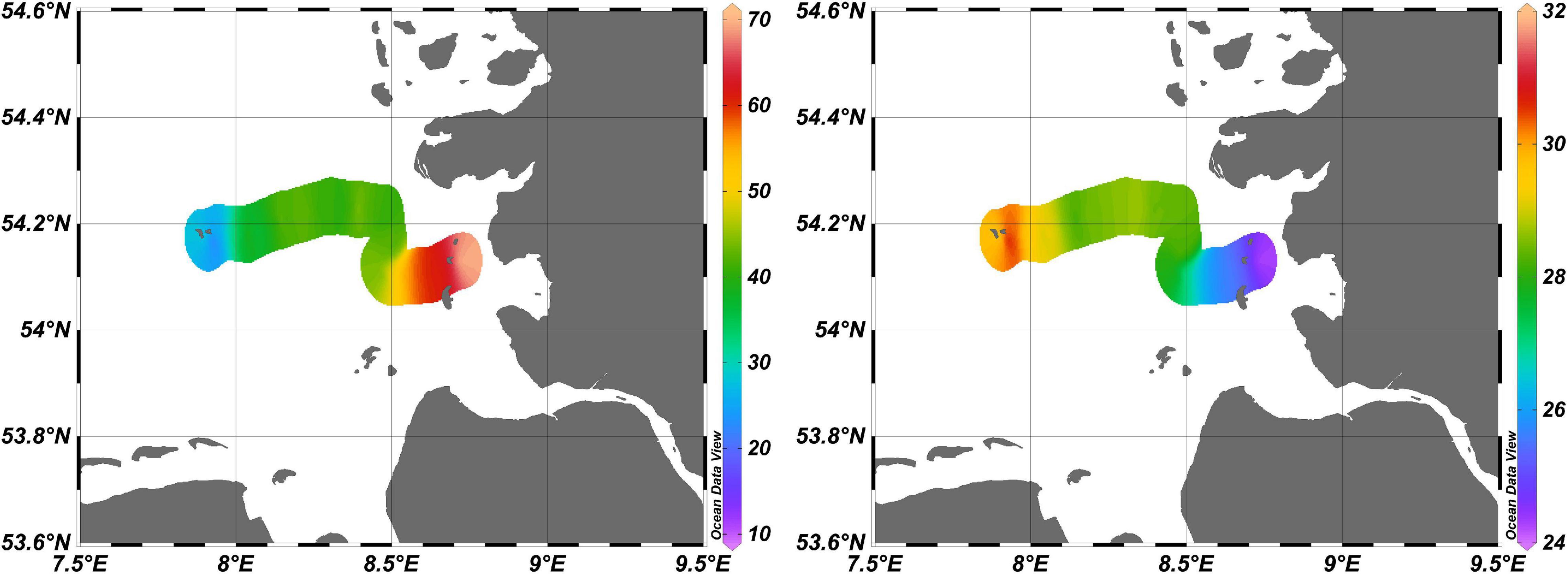
Figure 13. Distributions of surface NO₃^– concentrations (μM) obtained using the OPUS sensor (left panel) and surface salinity values recorded by the CTD (right panel) during the Sternfahrt-1 expedition. Color bars represent the levels of NO₃^– (left) and salinity (right) data.

A deep ocean field demonstration took place during the M158 research expedition in the tropical Atlantic Ocean in October 2019. The OPUS was mounted on a CTD frame and deployed with a vertical profiling speed of 1 m/s, which results in a vertical resolution of 2–3 m. The data presented here refers to the CTD71 deep cast deployment in which the OPUS sensor generated a total of 2,667 measurements (once every 3 s). A total of 13 discrete water samples were collected through closure of Niskin water samplers at various depths during the deployment. Vertical profiles of (1) NO₃^– concentrations derived from post-processing of the OPUS data with the OPUS coefficients (see section “Data Processing Procedure for OPUS”) and SUNA coefficients (TCSS algorithm and ε_{Br_cal}, ε_{NO3_cal} values from Sakamoto et al., 2009; Johnson et al., 2018) and discrete water samples analyzed in the laboratory, (2) temperature, salinity, and (3) ancillary data (phosphate, silicate, and dissolved oxygen) are presented in Figure 14. The OPUS data were obtained during the upcast and downcast profiles, while discrete water samples were collected only during the upcast profile. The OPUS NO₃^– data presented in Figure 14 are independent of an offset correction (i.e., adding the NO₃^– bias determined in surface waters to the rest of the data) and averaging. The mean and SD of 18 replicate measurements at the shallowest depth of this cast (27 m) is 0.16 ± 0.67 μM NO₃^–, and 18 replicate measurements at the deepest depth (3,905 m) is 22.24 ± 0.97 μM NO₃^–.

FIGURE 14

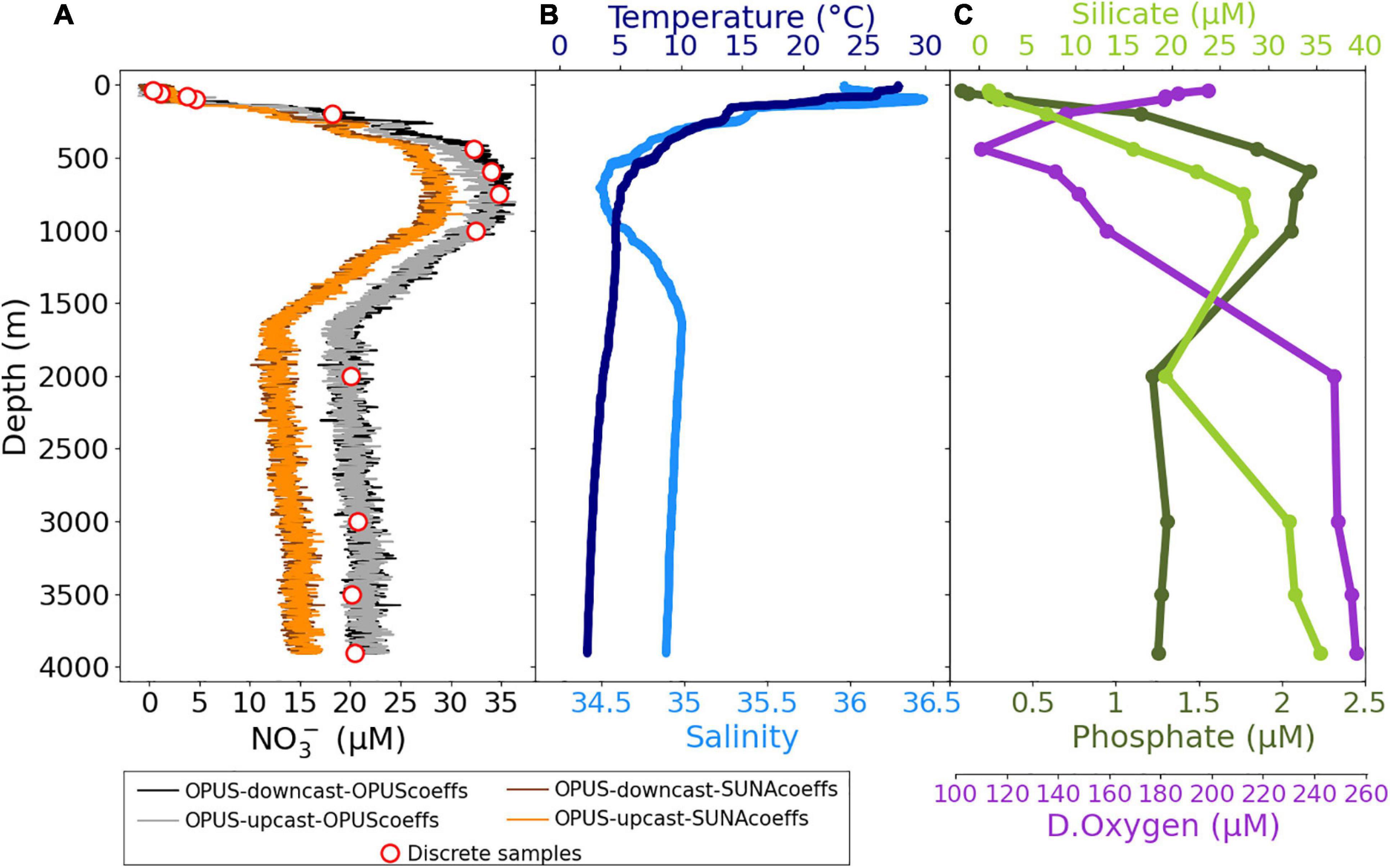
Figure 14. Vertical profiles of (A) NO₃^– concentrations (μM), (B) in situ temperature (°C), and salinity, (C) silicate (μM), phosphate (μM), and dissolved oxygen (μM) for cruise M158 cast CTD71 (00°00.00′S, 30°00.00′W). Black lines show NO₃^– values of the post-processed OPUS data obtained during the downcast, gray lines show NO₃^– values of the upcast profile, and red circles are for the discrete water samples analyzed in the laboratory by the wet chemistry–based method. Brown and orange lines are for the NO₃^– values of the post-processed OPUS data with the SUNA coefficients (Johnson et al., 2018).

Temperature values ranged between 2.3 and 27.7°C, and salinity between 34.4 and 36.4, characteristic of the hydrographic situation in the water column of the tropical Atlantic. The observed silicate values were between 1.02 and 35.3 μM, phosphate were from 0.07 to 2.17 μM, and dissolved oxygen levels were from 112 to 258 μM. The NO₃^– concentrations increased with depth toward the thermocline, from below the detection limit of the sensor (2 μM) in the surface mixed layer to 36 μM at 800 m depth and then decreasing to 20–23 μM below 2,000 m (see NOAA-NODC, 2018 for literature comparison; NO₃^– concentrations in October at surface, 800 m, and 4,000 m are ca. 0, 35, and 22 μM, respectively).

The sensor and discrete water samples data followed a broadly consistent pattern throughout the deployment period. Direct adaptation of SUNA coefficients resulted in bias in NO₃^– values of ca. 6 μM (Figure 14). Results indicate that improving the calibration and data processing procedure of the OPUS by deriving specific OPUS coefficients (Eq. 4 and OPUS-specific calibration file) increases the reliability of the NO₃^– data when compared with discrete water samples. The time of the sampling was precisely matched to a sensor measurement. However, a bias in NO₃^– was observed below 500 m (Figure 14) and attributed to specific optical characteristics of the sensor, which can be corrected by modifying wavelength offset and pressure factor (Pasqueron de Fommervault et al., 2015).

The sensor NO₃^– data presented throughout the study was post-processed with a wavelength offset of 210 nm (wo in Eq. 4), pressure factor of 0.026 (P_F in Eq. 5), and calibration file recorded at 20°C. Figure 15 shows an example of the impact of wo from 206 to 212, pressure factor of 0.020 (at wo = 210), and calibration file recorded at 5°C (at wo = 210) on the deviation of NO₃^– for the M158-CTD71 cast data. Using a lower wo with respect to the reference value of 210 nm results in lower NO₃^– values at temperatures below 20°C and higher NO₃^– values at temperatures above 20°C. Because our laboratory and field data are not adequate/sufficient for direct determination and quantification of the pressure dependence of Br^– spectra for the OPUS sensor, adaptation of the pressure factor of 0.020 (Pasqueron de Fommervault et al., 2015) can be advantageous to eliminate the overestimated NO₃^– at deep waters. Another reason for the deviation in NO₃^– could be related to the sharp temperature decrease, from 27.7 to 2.3°C, over short time scales (1 h), which might have affected the lamp output. The intensity of a xenon flash lamp changes with fluctuations in ambient temperature due to the fact that the gas pressure inside the bulb is temperature dependent; at 25°C, the intensity is 100% and decreases with decreasing temperatures (Hamamatsu Photonics, 2005). Determination of the stability of the lamp with respect to temperature was beyond the scope of the study; however, reference water-based spectra recorded at temperatures close to the sampled environment (i.e., 5°C) might be used for data below 500 m to minimize the dispersion.

FIGURE 15

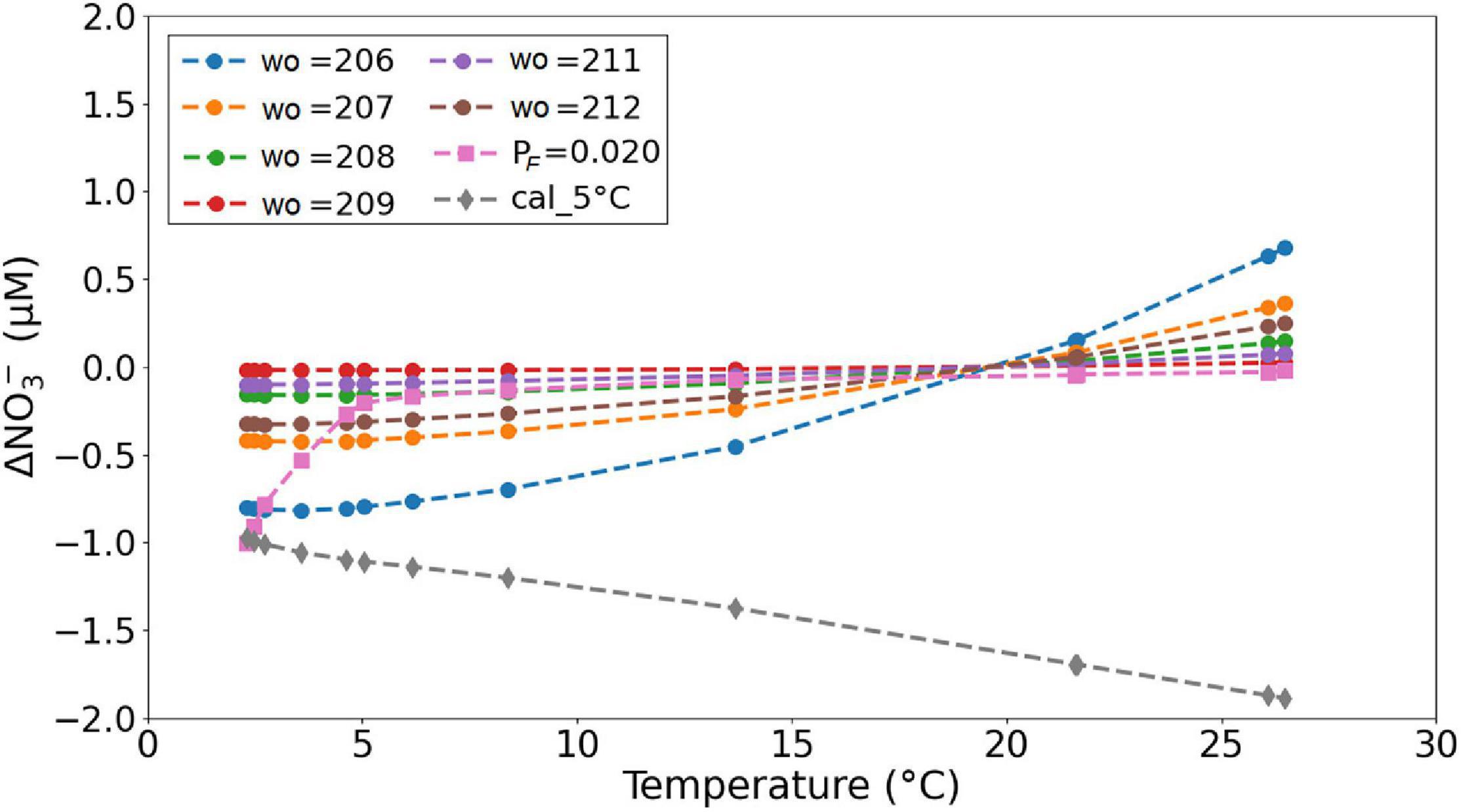
Figure 15. Deviation of the NO₃^– estimation with a wo of 210 nm, P_F of 0.026, and calibration file recorded at 20°C (OPUS-coefficients data presented in Figure 14A) as a function of in situ sample temperature. The results for P_F = 0.020 and calibration at 5°C were obtained at wo = 210.

The slight increase in sensor NO₃^– values with depth between 2,000 and 4,000 m shown in Figure 14 is unlikely to be a temperature effect because at these depths the measured temperature decrease was from 3.6 to 2.3°C and a comparison of the 20 and the 5°C calibration curves in Figure 15 suggests only a weak temperature effect (∼0.1 μM). Thus, a pressure effect on NO₃^– bias is more likely, and the NO₃^– values at depths are more vertical when processed with P_F = 0.020 than with P_F = 0.026 for the M158-CTD71 data presented (Figure 16).

FIGURE 16

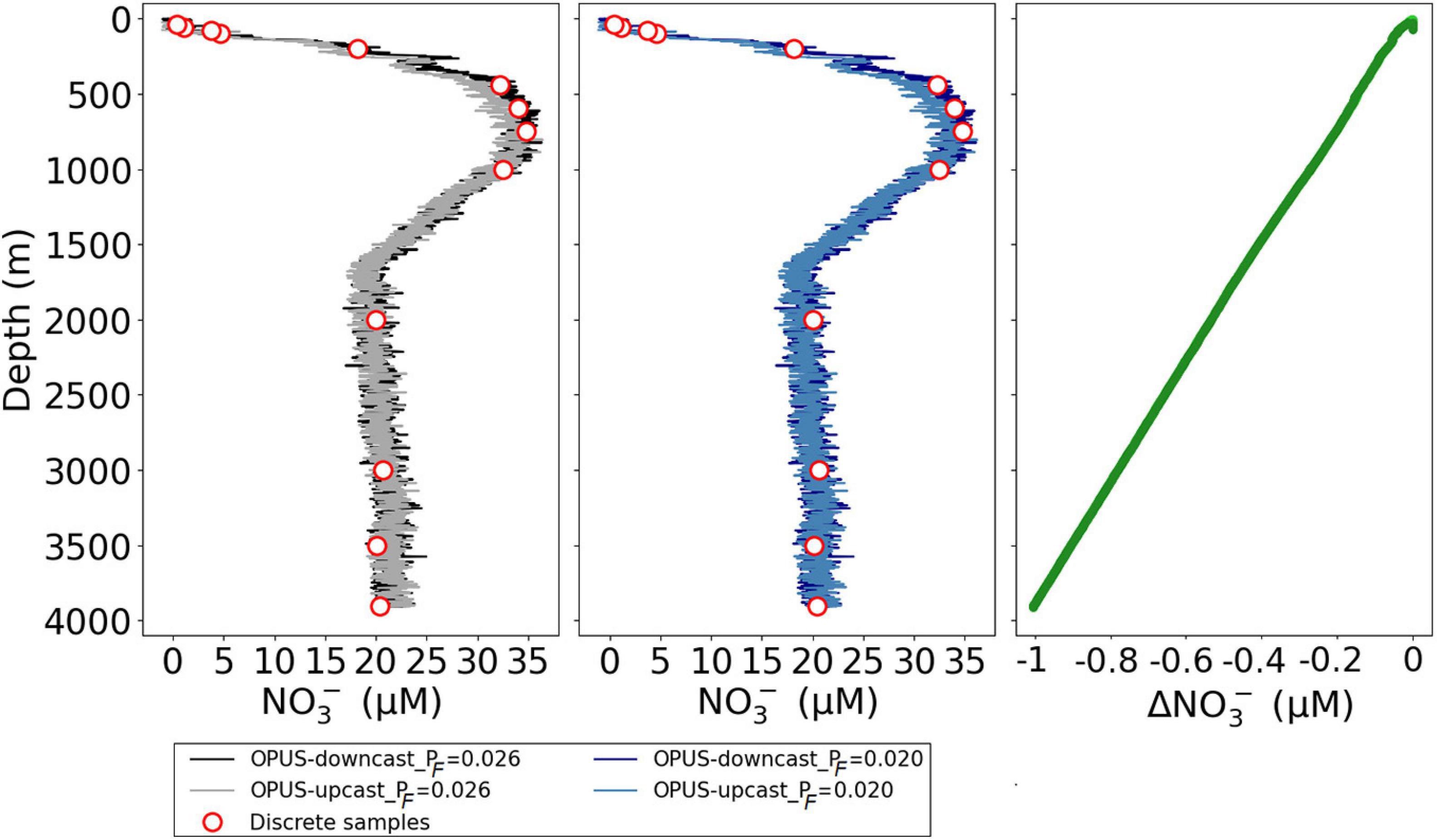
Figure 16. Vertical profiles of NO₃^– concentrations (μM) for cruise M158 and cast CTD71, in which the sensor data were processed using both P_F = 0.026 (left panel, black and gray lines) and P_F = 0.020 (middle panel, dark and light blue lines). The offset between them is presented in the right panel; ΔNO₃^– refers to the sensor NO₃^– data obtained with P_F 0.020-obtained with 0.026. Red circles are for the discrete water samples analyzed in the laboratory (see also Figure 14).

The fast sampling interval of the sensor was advantageous for a better spatial resolution of NO₃^– concentrations in the water column compared with discrete water samples. The OPUS sensor successfully captured the NO₃^– dynamics in the water column, agreeing with the values of discrete water samples analyzed in the laboratory during both field tests; the Sternfahrt-1 and the M158. A paired t-test confirmed no statistically significant differences (p ≤ 0.05) between NO₃^– values obtained from the sensor and discrete samples. A linear regression yielded y = 0.99x + 0.65 (r² = 0.99, n = 24) for the Sternfahrt-1 and y = 0.95x + 0.26, (r² = 0.99, n = 13) for the M158 data (Figure 17). The residuals of the fit are shown in Figure 17. The results indicated lower residual values for the open ocean deployment when compared with the coastal water deployment, and the maximum value for both cases was <2 μM NO₃^–.

FIGURE 17

Figure 17. Regression plots of NO₃^– concentrations determined in situ with the OPUS sensor vs. in the laboratory via autoanalyzer and residuals of the regression for the M158 data (A,B, see also Figure 14) and Sternfahrt-1 data (C,D, Figure 12).

The coastal waters can be high in dissolved organic materials that may interfere with optical NO₃^– determination. Although the algorithm (see section “Data Processing Procedure for OPUS”) performs a CDOM correction (Eq. 8), the high and variable content of CDOM might have partly affected the nitrate outputs. We used the difference in NO₃^– concentrations between the sensor and discrete water samples vs. the total absorbance in the CDOM wavelength range (240–260 nm) to check whether the NO₃^– bias is CDOM related, but no significant relationship was found (not shown here). Time series of measured absorbance at 254 nm and at 360 nm (wavelengths outside of the NO₃^– detection range) can be used to check anomalies related to yellow substances and particles, respectively. We checked this for both deployments data presented and found stable absorbances over time below <0.5 AU at 254 and 360 nm. Further investigation on the impact of yellow substances and particles on optical nitrate measurements in regions with a high organic matter content is needed. The effect of path length, as well as CDOM, on optical NO₃^– measurements were reported in detail by Snazelle (2016). The absorbance is directly proportional to path length. Another option could indeed be the use of a 5 mm or smaller path length instead of 10 mm.

The sensor measurements at the two shallowest depths, where the NO₃^– levels are below 2 μM, can be improved by small adjustments in data processing parameters as shown in Figure 15. We would like to mention that this is the first demonstration of a deep deployment of the OPUS sensor and so the initial step for future investigations such as an OPUS-specific pressure correction factor. Pressure-dependent experiments require more sophisticated experimental setups (Sakamoto et al., 2017).

Overall, the laboratory and field data presented throughout the study verified the success of the improvement work on calibration and data processing procedures of the OPUS.

Conclusion

This work highlights that the OPUS sensor is a useful tool to determine NO₃^– dynamics in the water column in real time by providing high-resolution in situ data, and thereby provides strong advantages over traditional laboratory analysis of discrete water samples. The data processing strategies of the OPUS described in this study strongly improved the quality of the sensor’s NO₃^– data output, and resulted in a comparable quality with the ISUS and SUNA sensors, with an accuracy of ∼2 μM and short-term precision of 0.4 μM NO₃^–. An inter-comparison between five OPUS sensors deployed in parallel under identical laboratory conditions showed no significant difference between the sensors. Deployment in coastal surface waters and the deep ocean demonstrated that the OPUS sensor can capture spatial variations across short spatial scales with results that were in excellent agreement with discrete water samples analyzed in the laboratory. The firmware design of the OPUS sensor is not suitable for a faster sampling rate than 3 s. Although the sampling rate of 3 s translates to a vertical resolution of 2–3 m, the sensor is advantageous due to the depth range of 6,000 m and it is the deepest operating optical nitrate sensor available for the research community. Another advantage of the OPUS are the long periods between lamp replacements. The previous version of the OPUS sensor named as ProPS was using a deuterium lamp and had a lifetime of 2 years, at 20°C and 15-min sampling interval. The expected lifetime of the OPUS is above 10 years, at 20°C with 1-min sampling interval (communication from manufacturer). Besides, the cost of the OPUS sensor (in Europe, about 10–12 k €) is considerably lower compared with other commercial UV nitrate sensors (i.e., SUNA about >40 k €) and therefore economically more affordable, especially for EU customers. The OPUS sensor is promising for future oceanographic studies. This study provides new insights specific for the OPUS sensors in the form of an “Ocean Best Practice” approach. Future work will focus on the assessment of the long-term performance of the OPUS on marine autonomous platforms, such as FerryBox systems and deep-sea gliders.

Data Availability Statement

The raw data supporting the conclusions of this article will be made available by the authors, without undue reservation.

Author Contributions

EA and MN conceptualized the study and methodology. CB and OZ supported the experimental tools. CB provided the initial Matlab scripts and assisted in the development of the OPUS controller. ME assisted during laboratory and field tests. MN wrote the article with edits and contributions from all co-authors.

Funding

This study was supported by funding to EA from the European Union’s Horizon 2020 Research and Innovation Program under the AtlantOS program, grant agreement no. 633211. EA acknowledges funding for the OCEANSensor project as part of the MARTERA Programme and financed by the German Federal Ministry of Economic Affairs and Energy (BMWi; Funding Agreement 03SX459A). Additional funding for OZ was acknowledged from SpectralArgo-N (BMBF; Funding Agreement 03F0825A).

Conflict of Interest

The authors declare that the research was conducted in the absence of any commercial or financial relationships that could be construed as a potential conflict of interest.

Acknowledgments

We would like to thank our colleagues André Mutzberg (GEOMAR) for analyzing discrete water samples for nutrients, and Dr. Gerd Krahmann (GEOMAR) for providing the M158 raw data. We also thank TriOS GmbH for their assistance in implementing high-resolution analysis mode.

References

Beaton, A. D., Cardwell, C. L., Thomas, R. S., Sieben, V. J., Legiret, F. E., Waugh, E. M., et al. (2012). Lab-on-chip measurement of nitrate and nitrite for in situ analysis of natural waters. Environ. Sci. Technol. 46, 9548–9556. doi: 10.1021/es300419u

PubMed Abstract | CrossRef Full Text | Google Scholar

Becker, S., Aoyama, M., Woodward, E. M. S., Bakker, K., Coverly, S., Mahaffey, C., et al. (2020). GO-SHIP repeat hydrography nutrient manual: the precise and accurate determination of dissolved inorganic nutrients in seawater, using continuous flow analysis methods. Front. Mar. Sci. 7:581790. doi: 10.3389/fmars.2020.581790

CrossRef Full Text | Google Scholar

Bittig, H. C., Maurer, T. L., Plant, J. N., Schmechtig, C., Wong, A. P. S., Claustre, H., et al. (2019). A BGC-argo guide: planning, deployment, data handling and usage. Front. Mar. Sci. 6:502. doi: 10.3389/fmars.2019.00502

CrossRef Full Text | Google Scholar

Burster Präezisionsmesstechnik GmbH. (2010). Precision Thermometer KELVIMATModel 4323. Gernsbach: Burster Präezisionsmesstechnik GmbH & Co. KG.

Google Scholar

Chegini, F., Holtermann, P., Kerimoglu, O., Becker, M., Kreus, M., Klingbeil, K., et al. (2020). Processes of stratification and destratification during an extreme river discharge event in the german bight ROFI. J. Geophys. Res. Ocean 125:e2019JC015987. doi: 10.1029/2019JC015987

CrossRef Full Text | Google Scholar

Claustre, H., and Johnson, K. S. (2019). 8th BGC Argo Data Management. Villefranche-sur-Mer. Available online: http://www.argodatamgt.org/content/download/33595/230003/file/BGC8_reports.pdf (accessed January 5, 2021).

Google Scholar

Daniel, A., Laës-Huon, A., Barus, C., Beaton, A. D., Blandfort, D., Guigues, N., et al. (2020). Toward a harmonization for using in situ nutrient sensors in the marine environment. Front. Mar. Sci. 6:773. doi: 10.3389/fmars.2019.00773

CrossRef Full Text | Google Scholar

Ey, S., Sm, K., Boersma, M., and Kh, W. (2017). Variations of annual turnover cycles for nutrients in the north sea, german bight nutrients turnover cycles in the north sea. Oceanogr. Fish. Open Access J. 2:555600. doi: 10.19080/OFOAJ.2017.02.555600

CrossRef Full Text | Google Scholar

Finch, M. S., Hydes, D. J., Clayson, C. H., Weigl, B., Dakin, J., and Gwilliam, P. (1998). A low power ultra violet spectrophotometer for measurement of nitrate in seawater: introduction, calibration and initial sea trials. Anal. Chim. Acta 377, 167–177. doi: 10.1016/S0003-2670(98)00616-3

CrossRef Full Text | Google Scholar

Frank, C., Meier, D., Voß, D., and Zielinski, O. (2014). Computation of nitrate concentrations in coastal waters using an in situ ultraviolet spectrophotometer: behavior of different computation methods in a case study a steep salinity gradient in the southern North Sea. Methods Oceanogr. 9, 34–43. doi: 10.1016/j.mio.2014.09.002

CrossRef Full Text | Google Scholar

Grasshoff, K. M., Erhardt, K. M., and Kremling, K. (1983). Methods of Seawater Analysis. Weinheim: Verlag Chemie.

Google Scholar

Guenther, E. A., Johnson, K. S., and Coale, K. H. (2001). Direct ultraviolet spectrophotometric determination of total sulfide and iodide in natural waters. Anal. Chem. 73, 3481–3487. doi: 10.1021/ac0013812

PubMed Abstract | CrossRef Full Text | Google Scholar

Hamamatsu Photonics, K. K. (2005). Xenon Flash Lamps. Available online at: http://educypedia.karadimov.info/library/Xe-F_TLSX9001E05.pdf. (accessed November 23, 2020).

Google Scholar

IOCCP (2017). Essential Ocean Variables (EOV): Nutrients, Global Ocean Observing System. Available online at: www.goosocean.org/eov (accessed February 4, 2020)

Google Scholar

Johnson, K. S. (2010). Simultaneous measurements of nitrate, oxygen, and carbon dioxide on oceanographic moorings: observing the redfield ratio in real time. Limnol. Oceanogr. 55, 615–627. doi: 10.4319/lo.2009.55.2.0615

CrossRef Full Text | Google Scholar

Johnson, K. S., and Coletti, L. J. (2002). In situ ultraviolet spectrophotometry for high resolution and long-term monitoring of nitrate, bromide and bisulfide in the ocean. Deep Sea Res. 1 Oceanogr. Res. Pap. 49, 1291–1305. doi: 10.1016/S0967-0637(02)00020-1

CrossRef Full Text | Google Scholar

Johnson, K. S., Coletti, L. J., Jannasch, H. W., Sakamoto, C. M., Swift, D. D., and Riser, S. C. (2013). Long-term nitrate measurements in the ocean using the in situ ultraviolet spectrophotometer: sensor integration into the APEX profiling float. J. Atmos. Ocean. Technol. 30, 1854–1866. doi: 10.1175/JTECH-D-12-00221.1

CrossRef Full Text | Google Scholar

Johnson, K., Pasqueron De Fommervault, O., Serra, R., D’Ortenzio, F., Schmechtig, C., Claustre, H., et al. (2018). Processing Bio-Argo Nitrate Concentration at the DAC Level. Villefranche-sur-Mer: Argo Data Management. doi: 10.13155/46121

CrossRef Full Text | Google Scholar

Jortner, J., Ottolenghi, M., and Stein, G. (1964). On the photochemistry of aqueous solutions of chloride, bromide, and iodide ions. J. Phys. Chem. 68, 247–255. doi: 10.1021/j100784a005

CrossRef Full Text | Google Scholar

Kristiansen, S., Farbrot, T., and Naustvoll, L.-J. (2001). Spring bloom nutrient dynamics in the Oslofjord. Mar. Ecol. Prog. Ser. 219, 41–49. doi: 10.3354/meps219041

CrossRef Full Text | Google Scholar

Mack, J., and Bolton, J. R. (1999). Photochemistry of nitrite and nitrate in aqueous solution: a review. J. Photochem. Photobiol. A Chem. 128, 1–13. doi: 10.1016/s1010-6030(99)00155-0

CrossRef Full Text | Google Scholar

Meyer, D., Prien, R. D., Rautmann, L., Pallentin, M., Waniek, J. J., and Schulz-Bull, D. E. (2018). In situ determination of nitrate and hydrogen sulfide in the baltic sea using an ultraviolet spectrophotometer. Front. Mar. Sci. 5:431. doi: 10.3389/fmars.2018.00431

CrossRef Full Text | Google Scholar

Morris, A. W., and Riley, J. P. (1966). The bromide/chlorinity and sulphate/chlorinity ratio in sea water. Deep Sea Res. Ocean. 13, 699–705. doi: 10.1016/0011-7471(66)90601-2

CrossRef Full Text | Google Scholar

Nehir, M., Frank, C., Aßmann, S., and Achterberg, E. P. (2019). Improving optical measurements: non-linearity compensation of compact charge-coupled device (ccd) spectrometers. Sensors 19:2833. doi: 10.3390/s19122833

PubMed Abstract | CrossRef Full Text | Google Scholar

NOAA-NODC. (2018). National Centers for Environmental Information, World Ocean Atlas 2018 (WOA18). Available online at: https://www.nodc.noaa.gov/cgi-bin/OC5/woa18f/woa18oxnuf.pl?parameter=n (accessed December 7, 2020).

Google Scholar

Ogura, N., and Hanya, T. (1966). Nature of ultra-violet absorption of sea water. Nature 212:758. doi: 10.1038/212758a0

CrossRef Full Text | Google Scholar

Pasqueron de Fommervault, O., D’Ortenzio, F., Mangin, A., Serra, R., Migon, C., Claustre, H., et al. (2015). Seasonal variability of nutrient concentrations in the Mediterranean Sea: contribution of bio-argo floats. J. Geophys. Res. Ocean. 120, 8528–8550. doi: 10.1002/2015JC011103

CrossRef Full Text | Google Scholar

Pellerin, B. A., Bergamaschi, B. A., Downing, B. D., Saraceno, J. F., Garrett, J. D., and Olsen, L. D. (2013). Optical techniques for the determination of nitrate in environmental waters: guidelines for instrument selection, operation, deployment, maintenance, quality assurance, and data reporting. U.S. Geol. Surv. Tech. Methods B 1:37.

Google Scholar

Pellerin, B. A., Saraceno, J. F., Shanley, J. B., Sebestyen, S. D., Aiken, G. R., Wollheim, W. M., et al. (2012). Taking the pulse of snowmelt: in situ sensors reveal seasonal, event and diurnal patterns of nitrate and dissolved organic matter variability in an upland forest stream. Biogeochemistry 108, 183–198. doi: 10.1007/s10533-011-9589-8

CrossRef Full Text | Google Scholar

Pidcock, R., Srokosz, M., Allen, J., Hartman, M., Painter, S., Mowlem, M., et al. (2010). A novel integration of an ultraviolet nitrate sensor on board a towed vehicle for mapping open-ocean submesoscale nitrate variability. J. Atmos. Ocean. Technol. 27, 1410–1416. doi: 10.1175/2010JTECHO780.1

CrossRef Full Text | Google Scholar

Prien, R. (2007). “Technologies for new in situ chemical sensors. In OCEANS 2007– - Europe, 2007. In OCEANS 2007 - Europe, 2007,” in IEEE, Proceedings of the International Conference on Marine Challenges: From Coastline to Deep Sea, Aberdeen, UK, (Aberdeen). doi: 10.1109/OCEANSE.2007.4302222

CrossRef Full Text | Google Scholar

Rieger, L., Langergraber, G., Kaelin, D., Siegrist, H., and Vanrolleghem, P. A. (2008). Long-term evaluation of a spectral sensor for nitrite and nitrate. Water Sci. Technol. 57, 1563–1569. doi: 10.2166/wst.2008.146

PubMed Abstract | CrossRef Full Text | Google Scholar

Sakamoto, C. M., Johnson, K. S., Coletti, L. J., and Jannasch, H. W. (2009). Improved algorithm for the computation of nitrate concentrations in seawater using an in situ ultraviolet spectrophotometer. Limnol. Oceanogr. Methods 7, 132–143. doi: 10.1002/lom3.10209

CrossRef Full Text | Google Scholar

Sakamoto, C. M., Johnson, K. S., Coletti, L. J., and Jannasch, H. W. (2017). Pressure correction for the computation of nitrate concentrations in seawater using an in situ ultraviolet spectrophotometer. Limnol. Oceanogr. Methods 15, 897–902. doi: 10.4319/lom.2009.7.132

CrossRef Full Text | Google Scholar

Sanders, T., Schöl, A., and Dähnke, K. (2018). Hot spots of nitrification in the elbe estuary and their impact on nitrate regeneration. Estuaries Coasts 41, 128–138. doi: 10.1007/s12237-017-0264-8

CrossRef Full Text | Google Scholar

Sea-Bird Coastal SUNA. (2015). Submersible Ultraviolet Nitrate Analyzer (SUNA) User Manual Edition 1. Bellevue, WA: Sea-Bird Scientific.

Google Scholar

Snazelle, T. T. (2016). The Effect of Suspended Sediment and Color on Ultraviolet Spectrophotometric Nitrate Sensors. U.S. Geological Survey, Open-File Report, 2016–1014. 10. Available online: https://pubs.er.usgs.gov/publication/ofr20161014 (accessed October 10, 2020).

Google Scholar

Stedmon, C. A., and Nelson, N. B. (2015). “The optical properties of dom in the ocean,” in Biogeochemistry of Marine Dissolved Organic Matter, eds D. A. Hansell and C. A. Carlson (Amsterdam: Elsevier Inc), 481–508. doi: 10.1016/B978-0-12-405940-5.00010-8

CrossRef Full Text | Google Scholar

TriOS GmbH. (2017). OPUS Operating Instructions. Rastede: TriOS Mess- und Datentechnik.

Google Scholar

van Beusekom, J. E. E. (2018). “Eutrophication,” in Handbook on Marine Environment Protection, eds M. Salomon and T. Markus (Cham: Springer), 429–445.

Google Scholar

Voynova, Y. G., Brix, H., Petersen, W., Weigelt-Krenz, S., and Scharfe, M. (2017). Extreme flood impact on estuarine and coastal biogeochemistry: the 2013 elbe flood. Biogeosciences 14, 541–557. doi: 10.5194/bg-14-541-2017

CrossRef Full Text | Google Scholar

Vuillemin, R., and Sanfilippo, L. (2010). A compact, low-power in-situ flow analyzer for marine applications. Sea Technol. 51, 29–32.

Google Scholar

Wong, C. S., Waser, N. A. D., Nojiri, Y., Whitney, F. A., Page, J. S., and Zeng, J. (2002). Seasonal cycles of nutrients and dissolved inorganic carbon at high and mid latitudes in the North Pacific Ocean during the Skaugran cruises: determination of new production and nutrient uptake ratios. Deep. Res. Part II Top. Stud. Oceanogr. 49, 5317–5338. doi: 10.1016/S0967-0645(02)00193-5

CrossRef Full Text | Google Scholar

Zielinski, O., Fiedler, B., Heuermann, R., Kortzinger, A., Kopiske, E., Meinecke, G., et al. (2007). “A New nitrate continuous observation sensor for autonomous sub-surface applications: technical design and first results. In OCEANS 2007– - Europe, 2007,” in IEEE, Proceedings of the International Conference on Marine Challenges: From Coastline to Deep Sea, Aberdeen, UK, 18–21 June 2007, (Aberdeen). doi: 10.1109/OCEANSE.2007.4302300

CrossRef Full Text | Google Scholar

Zielinski, O., Voß, D., Saworski, B., Fiedler, B., and Körtzinger, A. (2011). Computation of nitrate concentrations in turbid coastal waters using an in situ ultraviolet spectrophotometer. J. Sea Res. 65, 456–460. doi: 10.1016/j.seares.2011.04.002

CrossRef Full Text | Google Scholar