Detecting Climate Signals in Southern Ocean Krill Growth Habitat

Introduction

The Southern Ocean, which surrounds Antarctica, is a critical component of the Earth system and supports a marine ecosystem of immense economic and intrinsic value. It is also among the most sensitive areas to climate change (Hagen et al., 2007) and has already experienced physical changes in ocean temperature, sea-ice dynamics, stratification, and currents (Flores et al., 2012). The cumulative impact of these changes on the marine ecosystem and its primary keystone species, Antarctic krill (Euphausia superba), is predicted to increase considerably during the present century (Doney et al., 2012; McBride et al., 2014). However, in addition to trends forced by global-scale, human-driven warming, the Southern Ocean is also subject to highly-dynamic natural climate variability, which can exert important influence on the system on interannual to multi-decadal timescales (Mayewski et al., 2009). This research presents an analysis of the superposition of forced climate change and natural variability on Antarctic krill habitat. In the context of climate change and the highly dynamic Southern Ocean, the framework we present provides insights that are important for decision makers to consider regarding climate change adaptation strategies.

Antarctic krill (hereafter krill) are at the center of the Southern Ocean food web as well as the target of the largest commercial fishery in the Southern Ocean (Nicol et al., 2012). Krill are a large bodied (up to ∼6 cm), fast swimming, aggregating, zooplankton known as a dominant species in the food web and in biogeochemical cycles (Tarling and Fielding, 2016; Trathan and Hill, 2016; Cavan et al., 2019). Krill are one of the most abundant wild animal species on Earth, with a biomass estimated between 300 and 500 million tons (Nicol and Mangel, 2018). The rate at which krill biomass is produced, or productivity, is central to the success of the ecosystem; thus, changes in krill distribution and abundance have ramifications across the ecosystem (Murphy et al., 2012; Constable et al., 2014; Larsen et al., 2014). A wide variety of Antarctic species feed on krill and they are the main energy pathway connecting primary producers to higher order predators (Quetin and Ross, 2003; Atkinson et al., 2009; Schmidt et al., 2011). Localized industrial fishing efforts, however, are growing rapidly (Nicol et al., 2012) and remove krill biomass in direct competition with krill-dependent species. These ecological and economic activities, however, are situated in the context of a highly dynamic climate system. Climate variability and change has the potential to drive important fluctuations in krill biomass, yielding widespread ecological impacts and causing variations in the definition of sustainable catch. Prediction of climate variability and change is therefore of high importance for effective long-term management of the ecosystem.

Concerns over the ecosystem impacts of growing commercial fishing interest for krill in the 1980s spurred the creation of the Convention on the Conservation of Marine Living Resources (CCAMLR) to govern the Southern Ocean (Nicol et al., 2012). Since the early 2000s human interest in krill has been rising and now represents the largest fishery, by biomass, in the Southern Ocean (Nicol and Foster, 2016). The krill fishery is managed under a mandated precautionary, ecosystem-based approach—including managing for environmental change, and based on the best available science (Constable, 2000). Currently, krill are managed with catch limits that are deemed to be precautionary, however, these limits are set using a stock assessment that does not account for environmental variability or climate change impacts (Constable and Kawaguchi, 2018; Watters et al., 2020). Fisheries compete with natural predators for krill biomass, making coordinated management critical for sustaining the Antarctic marine ecosystem (Meyer et al., 2020; Watters et al., 2020). Variation in climate, however, independently affects krill productivity, yielding bottom-up fluctuations in krill biomass (Atkinson et al., 2019). Effective management of the krill fishery, therefore, depends on sound understanding of climate-driven variations in krill populations. This research is thus motivated to inform this critical gap in management regarding the impacts of natural variability and climate change.

Climate affects krill through direct impacts (e.g., physiological thresholds, habitat use) and indirect impacts such as ecosystem interactions, including impacts on food supply and predation. The influence of natural climate variability is a large factor in understanding krill abundance, distribution, and productivity. However, accurate measurements of krill biomass are sparse, making it difficult to develop mechanistic connections between possible environmental drivers and krill production. In spite of uncertainty regarding specific mechanistic connections, there is broad consensus that krill populations are likely to be impacted by future changes in climate (Murphy et al., 2012; Constable et al., 2014; Rogers et al., 2020; Veytia et al., 2020). Attributing trends in krill production to anthropogenic climate change is challenged by the confounding influence of natural variability on top of limited observational data. The Southern Ocean’s natural system is sufficiently dynamic such that important environmental fluctuations are likely even in the absence of human-driven warming.

It is critical to recognize that “climate” is not static, but rather manifests as a superposition of naturally-driven variability and human-driven trends (Hawkins and Sutton, 2009; Deser et al., 2012). Natural climate variability is an intrinsic feature of the earth system; it is attributable to nonlinear dynamical processes and interactions between climate system components that integrate information over different timescales (Hasselmann, 1976). Anthropogenic forcing from human-driven trends, like emissions of heat-trapping gases, externally forces the climate system. The characteristics of the superposition of internal variability on anthropogenic forcing in the Southern Ocean are illustrated by the Westerly Winds that drive the Antarctic Circumpolar Current (Allison et al., 2010) (Locations are referenced in Figure 1). The strength and position of the Westerlies naturally fluctuate in association with the Southern Annular Mode (Rogers and van Loon, 1982; Thompson and Wallace, 2000). Human-driven trends are superimposed on this variability: ozone depletion, followed by CO₂-driven warming has resulted in an intensification of the SAM index, a trend that is projected to continue over the next several decades (Fogt and Marshall, 2020; Goyal et al., 2021). Understanding the how, where, and by how much the fluctuations of natural variability may obscure observed trends (Ryabov et al., 2017) in anthropogenic climate change on different timescales is highly important for effective and long term resource management.

FIGURE 1

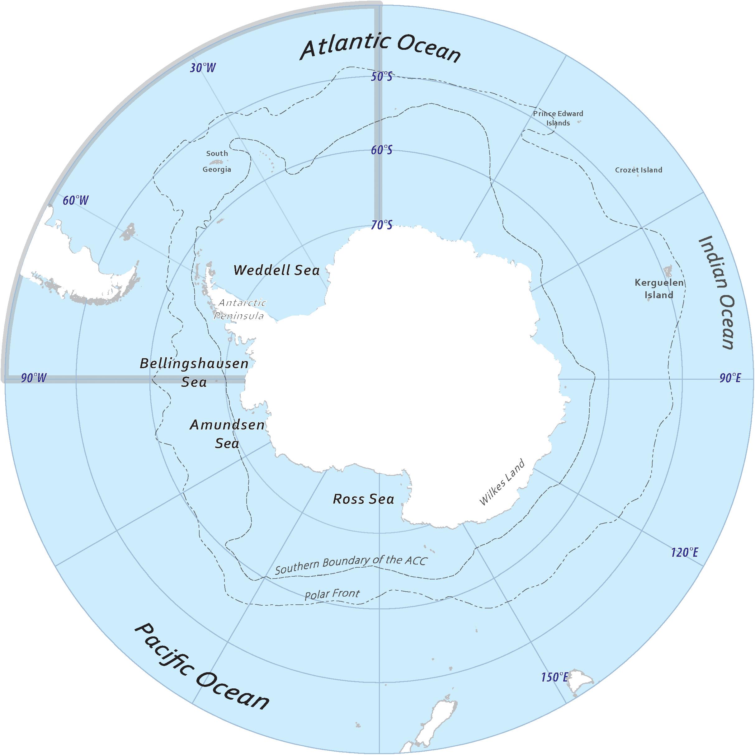
Figure 1. This map illustrates the study area containing the locations and features referenced throughout paper. Notably, the Atlantic quadrant is highlighted in gray as the area between 0° and 90°W. All spatially averaged data is constrained by the 45°S latitude. Figure prepared by ZS, frontal data from Orsi et al. (1995).

In the context of developing future projections, natural climate variability makes important contributions to uncertainty. Determining the uncertainty attributed to the two components of climate variability is a function of time horizons and scale (Commission on Geosciences, Environment, and Resources, Climate Research Committee, National Research Council, and Division on Earth and Life Studies, 1996). Internal variability is often the dominant source of uncertainty at regional scales or over less than two decades. Comparatively anthropogenic forcing is associated with longer-term trends at larger spatial scales (Hawkins and Sutton, 2009). When superimposed, fluctuations in natural variability have the potential to temporarily reverse or partially offset forced trends on interannual to decadal timescales. For example, in the western Atlantic Peninsula (WAP), the long term trend shows significant warming and sea ice loss overall (Henley et al., 2019) while short-term regional observations from the late 1990s and late 2000s showed a trend of increasing sea-ice extent (Stammerjohn et al., 2012). The long-term trend in the WAP was superimposed by significant natural variability in the regional climate resulting in short-term variation in sea ice dynamics (Hobbs et al., 2016; Turner et al., 2016; Stammerjohn and Maksym, 2017). Trends associated with the forced signal are unlikely to be reversed on short timescales or can only be reversed through intervention. Quantifying climate-change related impacts provides fundamental knowledge that can help inform management, including a framework for considering when and where to employ climate mitigation strategies.

Detection and attribution of forced trends must be approached against the backdrop of natural variability (Hawkins, 2011; Deser et al., 2012). Detecting trends and attributing them to forced climate change can be approached as a signal-to-noise problem: the forced trends represent a “signal” and the natural climate variability is “climate noise” (Feldstein, 2000). The forced signal will arise from the envelope of background climate noise if it is sufficiently large for an extended period of time (Hasselmann, 1993; Santer et al., 2011). A climate change signal is easier to detect in a system where the magnitude of the forced trends is large relative to the natural variability. The point in time when the anthropogenic climate change signal can be detected from the noise of internal climate variability is known as the “Time of Emergence” (ToE). Determining the ToE can help us determine if the state of the system is past the expected natural variability as well as what it could mean for the system to start to move outside of the noise of natural variability (Deser et al., 2012; Hawkins and Sutton, 2012; Bonan and Doney, 2018).

Assessing when expected changes can be detected or if observed changes can be attributed to the forced trend is challenging to address definitively through observational records alone (Deser et al., 2012; Hawkins and Sutton, 2012; Bonan and Doney, 2018). When either observational records are scarce, like in the Southern Ocean, or we want to observe the future, modeling studies can provide insight. Earth system models (ESMs) are climate models that include a variety of ecological processes with the aim of simulating a fully-prognostic global carbon cycle (e.g., Hurrell et al., 2013). While ESMs may have significant biases relative to observations, they are formulated on the basis of physical principles, conserve mass and energy, and are internally consistent. Through the ability to run multiple realizations of the climate system as it transits through different forcing scenarios, ESMs can be used to examine detection and attribution of trends associated with forced climate change. ESMs include ocean biogeochemistry models as a component of the carbon cycle. As ESMs have evolved, there has been increasing recognition of their relevance to questions beyond carbon biogeochemistry, and in particular related to ocean ecosystems in the context of climate variability and change (Stock et al., 2011; Bopp et al., 2013; Tommasi et al., 2017).

Prior research has used outputs from ESMs to explore how changes in Southern Ocean climate will impact regional and circumpolar krill habitat. These studies have mainly used projected changes from multi-model ensembles from the Coupled Model Intercomparison Project Phase 5 (CMIP5) in combination with empirically-derived models (Atkinson et al., 2006; Hill et al., 2013; Piñones and Fedorov, 2016; Veytia et al., 2020). However, these multi-model ensemble studies have not considered the role of naturally occurring internal climate variability. The large-ensemble framework of a single ESM allows for quantification of the uncertainties from internal variability, identifying trends forced by human-driven climate change and identifying when those trends can be formally distinguished from natural variability. This study expands upon the previous work by considering the distinct roles of forced climate change and natural variability in driving fluctuations in krill habitat. Thus, we present an approach to differentiate the impacts of internal variability from forced trends on krill growth rates, also referred to as growth potential (GP).

Materials and Methods

Earth System Model

We used output from the Community Earth System Model Large Ensemble (CESM-LE) (Kay et al., 2015). The model configuration included atmosphere, ocean, land, and sea ice component models based on a 1° horizontal integration (Hunke and Lipscomb, 2010; Danabasoglu et al., 2012; Holland et al., 2012; Lawrence et al., 2012). The CESM-LE began with multicentury, 1850-control simulation with constant preindustrial forcing; a single ensemble member was branched off this simulation and integrated from 1850 to 1920, at which point additional members were added. We used 28 members with ocean biogeochemistry output from the CESM-LE integrated over the period from 1920 to 2100, each using the same historical and future-scenario (RCP 8.5; Long et al., 2016) external forcing. Each ensemble member simulation has a unique climate trajectory because of small round-off level differences (10^–14 K) in the air temperature field at initialization in 1920 (Kay et al., 2015). The climate system is sufficiently chaotic that these small deviations grow rapidly, leading to substantial spread across the ensemble that reflects the amplitude of internally-generated variability. When an ensemble is sufficiently large, the ensemble mean provides a robust estimate of the deterministic response of the climate system to external forcing, i.e., the forced trend. The ensemble spread, then, is indicative of the “noise,” inclusive of changes in variance that may occur as a function of climate state (Deser et al., 2012; Long et al., 2016). The large ensemble framework therefore allows for assessment of internal climate variability relative to the magnitude of the forced anthropogenic change (Deser et al., 2012; Hawkins and Sutton, 2012; Lovenduski et al., 2016; Brady et al., 2017).

Most ESMs, including the CESM-LE, incorporate prognostic representations of zooplankton as a component of their ocean biogeochemistry simulation (Le Quéré et al., 2016). However, ESMs typically simplify diverse groups of planktonic organisms into plankton functional types (Quéré et al., 2005), which are delineated based on ecological or biogeochemical roles. ESMs do not typically simulate specific zooplankton species as state variables; moreover, krill are typically larger and have more complicated life-history than the included phytoplankton functional types. We use the ocean biogeochemistry model output from the CESM-LE to represent bottom-up drivers and apply the krill growth model from Atkinson et al. (2006) offline to quantify changes in krill growth potential over the duration of the simulation. Since the krill growth potential model is applied offline, this approach precludes representing feedbacks between krill potential and other aspects of the biogeochemical simulation.

Bias in mean state and variability of sea surface temperature (SST) and chlorophyll can dramatically affect the characteristics of the simulated krill growth potential due to the highly nonlinear krill growth potential equation, therefore it is important to understand the model’s ability to reproduce observed SST and chlorophyll during austral summer. To address this, we compared an austral summer (December through February, referred to as DJF) climatology from the CESM-LE to climatologies constructed from observational datasets and regridded onto the nominally-1° CESM ocean component grid (Figure 2). Surface chlorophyll data from September 1997 to December 2010 was obtained from SeaWiFS OC4v6 (NASA Ocean Biology Processing Group, 2018) (Figure 2a). SST observations from 1981 to 2015 were obtained from the Hadley Centre Global Sea Ice and SST (HadISST) dataset (Hadley Centre for Climate Prediction and Research, 2000) (Figure 2d). The SeaWiFs data set was used in the derivation of the original krill growth model (Atkinson et al., 2006) (Figure 2e). The simulated SST values were positively biased beyond the Polar Front and slightly negatively biased along the western Antarctic Peninsula and into the Scotia Sea region (Figure 2f). Chlorophyll in the model was positively biased along the coastlines from the Scotia Sea region to the Bellingshausen Sea region, to the Ross Sea region (Figure 2c). It was further determined that the model biases were not outside the range of reasonable natural variability, but should be considered in evaluating results.

FIGURE 2

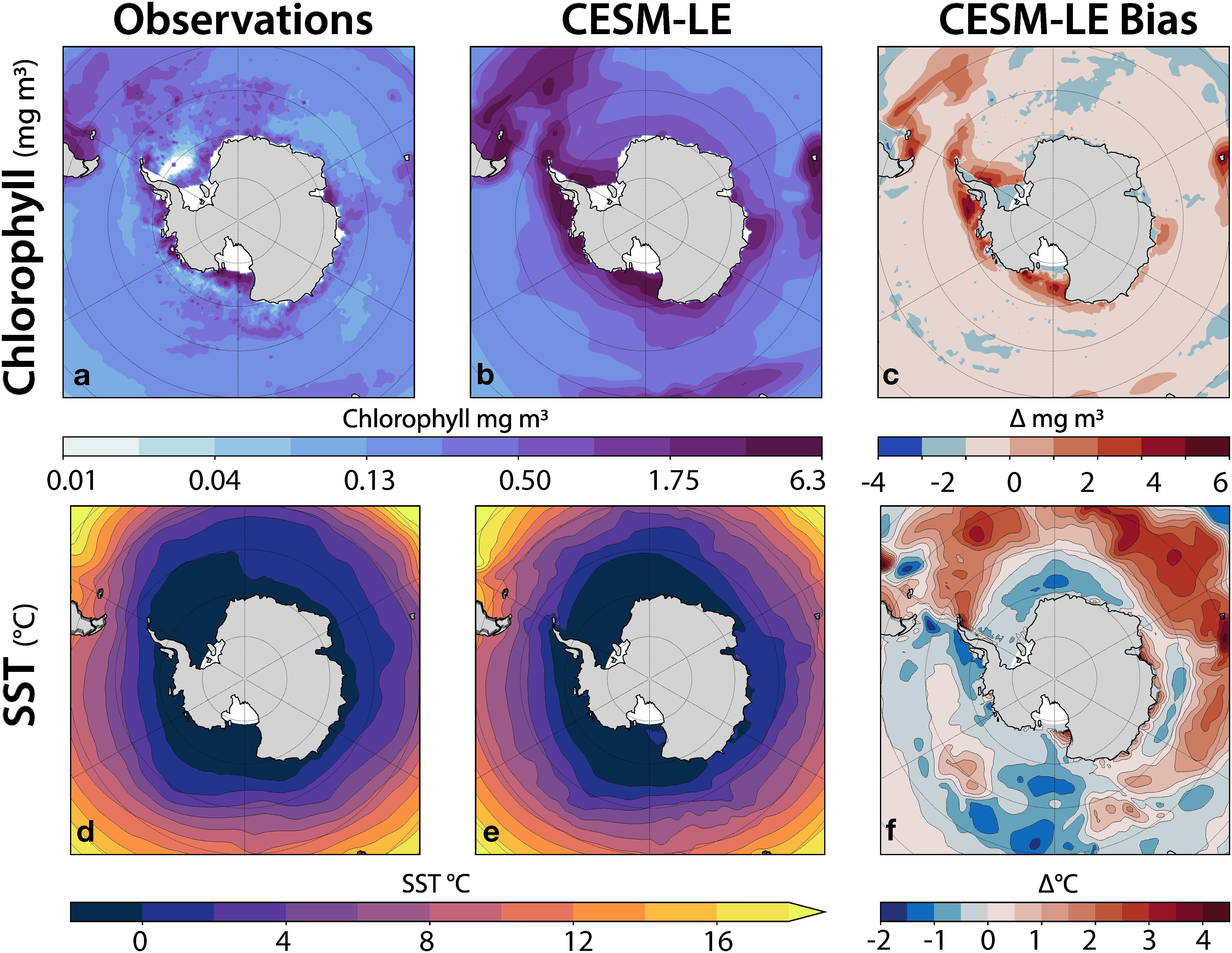
Figure 2. CESM-LE model bias in chlorophyll (top row) and SST (bottom row) for DJF (austral summer). The left column shows observations, the middle column shows the corresponding simulated CESM-LE fields, and the right column shows the simulated bias as the difference between the simulated fields and the observations.

Krill Growth Potential

This study coupled an existing empirical krill growth model with the CESM-LE. The empirical model from Atkinson et al. (2006) was used to estimate the daily growth rate of krill (DGR mm day^–1) from sea surface temperature (T_surf, °C), food availability, indicated by surface chlorophyll a concentration (Chl, mg m^–3), and starting length of krill (L, mm):

$$DGR=-0.006+0.002L-0.000061L^2+[0.385Chl/(0.328+Chl)]+0.0078T{}_{surf}-0.0101T{}_{surf}{}^2(1)$$

The model estimates a daily krill growth rate given temperature and the concentration of food in the summer season. The growth rate equation was derived using in-situ data from instantaneous growth rate experiments in the southwest Atlantic sector during the summer (January and February) of 2002 and 2003. It was further tested with SeaWiFS-derived chlorophyll to generate a predictive model of growth based on satellite-derivable environmental data (Atkinson et al., 2006). Previous studies have applied the growth model across the Southern Ocean at varying spatial and temporal scales to assess changes in habitat suitability (Hill et al., 2013; Murphy et al., 2017; Veytia et al., 2020). The growth rate provides a descriptive measurement of habitat suitability where a positive growth rate indicates habitat that can maintain and support adult krill productivity.

The variability of the environmental drivers (SST and chlorophyll) about a particular mean-state can dramatically affect the characteristics of the growth rate, due to the highly nonlinear nature of Eq. 1. While prior studies have used annual-mean climatologies to calculate GP rates results, we chose to calculate GP on monthly data (the highest frequency available from the model) to remain closer to the temporal resolution of the data used to develop the model. Seasonal estimates of krill GP at a starting length of an average adult krill (40 mm) were calculated from the growth period (December through February, referred to as DJF). The observed mean length of adult krill (40 mm) (Atkinson et al., 2009) was assumed as the starting length for an individual krill as previous analyses found that projected differences between future and historical epochs remained the same irrespective of starting length (Veytia et al., 2020). Krill GP was calculated as a rate of mm day^–1 where environmental conditions were within the temperature parameters that the growth model was derived from (−1 to 5°C).

The growth model predicts both positive and negative GP rates. Negative GP rates can occur when food concentrations are too low causing krill to undergo shrinkage (Hofmann and Lascara, 2000; Fach et al., 2002). Growth habitat was defined as habitat with a GP rate > 0 mm day^–1 where higher GP rates indicated that habitat was more supportive of increasing krill growth and thus of higher quality. Habitat with a GP rate ≤ 0 mm day^–1 was defined as “unsuitable habitat” where krill could survive but would not grow or where they would experience starvation and potentially undergo shrinkage.

Time of Emergence

We include a formal assessment of the time of emergence (ToE) of forced signals in the context of natural variability. ToE is the time when trends attributable to external forcing can be statistically distinguished from natural variability, which amounts to a signal to noise problem; detection is possible only when the magnitude of the forced response, the signal, exceeds the noise attributable to natural variability. Following Long et al. (2016), a time evolving spatial pattern of a variable in ensemble member i (ψ_i) is the sum of the internal variability and forced trend signal:

$${\mathrm{\psi }}_i={\mathrm{\psi }}_i^{\prime }+{\mathrm{\psi }}^s(2)$$

The forced climate signal is represented by ψ^s while the component due to internal variability is represented as ψ_i’. In the CESM-LE, the number of ensemble members (m) is sufficiently large (Deser et al., 2012) that an average across the ensemble provides a reasonable estimate of the forced signal, ψ^S:

$${\mathrm{\psi }}^s=\frac{1}{n}\sum _{i=1}^n{\mathrm{\psi }}_i(3)$$

To assess the temporal evolution of trends and normalize the data, anomalies were calculated by removing the ensemble mean of a representative period of unperturbed climate: 1920–1950, from each ensemble member. We adapted a ToE method (Henson et al., 2017) that computes the start of a climate change signal (inflection point), the trend in the climate change signal (ω), and the year of emergence of the signal (ToE). For each grid cell, across all ensemble members, the ensemble mean (ψ^s) was cumulatively integrated over time using the composite trapezoidal rule in order to identify the year when the start of the climate change signal began, or the ‘inflection point’. The ‘inflection point’ was defined as the year when the cumulative integral exceeded or dropped below zero (depending on the sign of the climate trend) for the remainder of the time series. With the inflection point identified, the trend of the climate change signal (ω) was calculated using a least squares polynomial fit function on the ensemble mean.

The timescale of the ToE was computed by multiplying the standard deviation of climate anomalies in the “unperturbed climate” (σ) by two and dividing it by the climate change trend (ω):

$$ToE=(2^{*}\mathrm{\sigma })/\mathrm{\omega }(4)$$

Using the ToE timescale, the year of detection was then calculated by adding the ToE to the starting year of the simulation, 1920 (T_detect = T₀ + ToE).

Results

In our examination of simulated GP distributions prior to significant influence from the forced trend, spatial patterns in the distribution of krill GP rates were closely related to their thermotolerance range during the summer season. GP habitat was found within the Atlantic sector (30–70°W) along the latitudinal bands around the South Orkney Islands and along the eastern coastal regions near Wilkes Land (90–120°E) (Figure 3a). Temperature exerted a strong control on GP, with elevated GP values typically found within the optimal temperature range (−1 to 2°C) and located in coastal regions with high chlorophyll concentrations. The distribution of growth habitat was strongly constrained on its northern boundary by the edge of the 5°C isotherm that coincides with the Polar Front of the Antarctic Circumpolar Current (ACC) (Figure 1). Habitat within krill’s thermotolerance with insufficient chlorophyll concentrations for growth (unsuitable habitat) were located in the Ross Gyre and Weddell Gyre and in the latitudinal range of the Polar Front (Figure 3e).

FIGURE 3

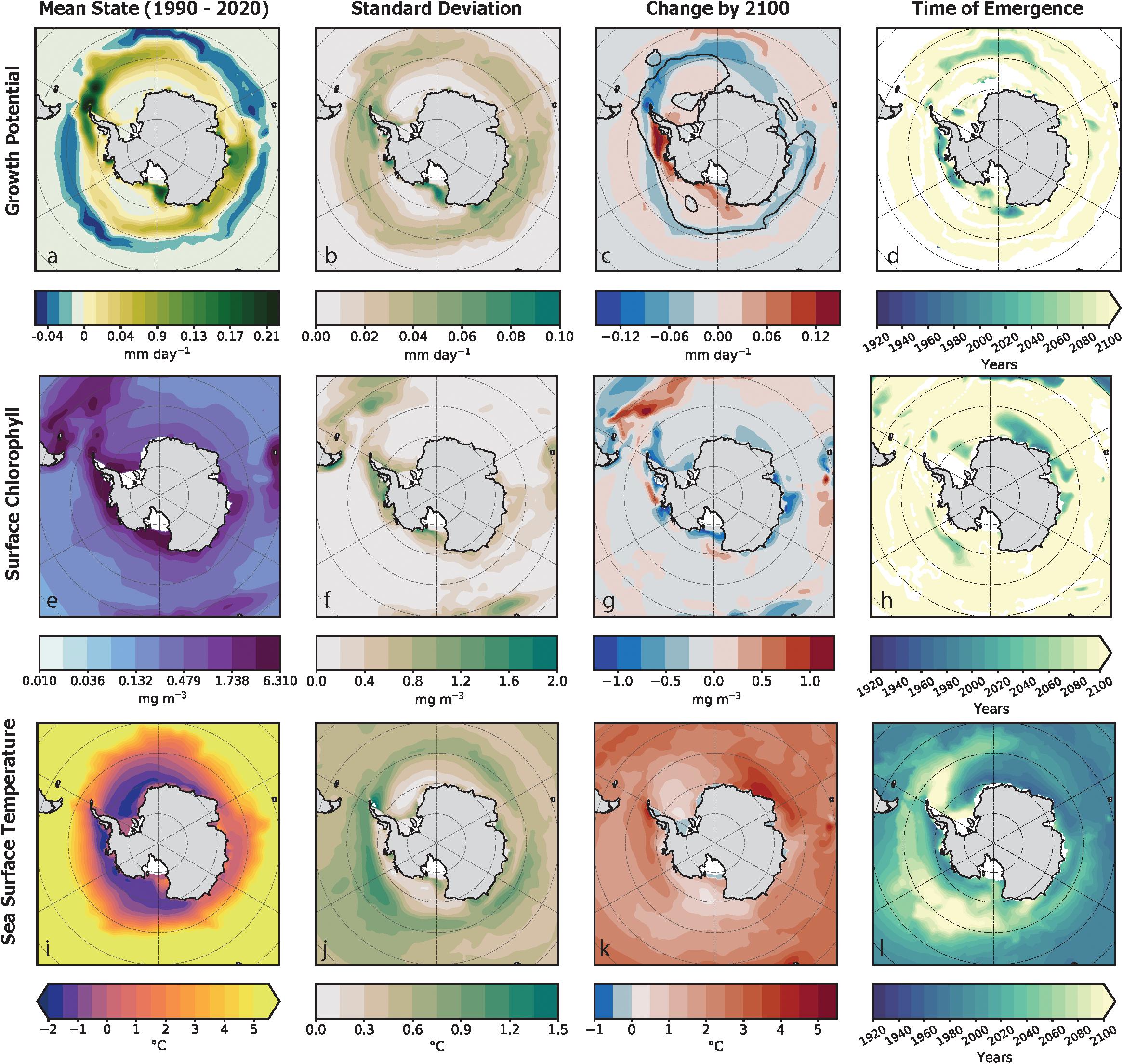
Figure 3. This figure captures the spatial characteristics in the mean state of krill growth potential [top row: (a–d)], chlorophyll [middle row: (e–h)] and sea surface temperature [bottom row: (i–l)] as simulated by the large ensemble for the austral summer period. The mean state for the current climate (1990–2020) of the is shown for each variable in the leftmost column. Plot (a) shows growth potential of krill habitat as the rate growth per day (mm day^–1) where habitat that can support krill growth is green and habitat where krill growth is inhibited is blue. The mean state of surface chlorophyll concentration (mg m^–3), as shown in plot (e), is plotted on a logarithmic scale. Plot (i) illustrates sea surface temperatures (SST) within the optimal temperature range that the empirical growth model was developed (Atkinson et al., 2006). The second column of plots to the left (b,f,j) shows the standard deviation of the mean state. The column second to the right (c,g,k) is the projected change in the forced signal from the unperturbed climate to the future climate. The difference is shown using a diverging color scale: increasing trends are shown in red and decreasing trends are shown in blue. In plot (c), a black contour line indicates the distribution of habitat with positive krill GP by 2100. The right most column (d,h,l) is the year of detection of the “time of emergence” of the forced trend for. Areas in white indicate habitat where a ToE could not be detected. Where the ToE could be detected, the earlier the year of the ToE the darker the color represented on the map.

The CESM-LE simulated a poleward contraction in growth habitat and an overall decline in the spatial average of krill GP over the course of the 21st century. The circumpolar habitat area with positive growth potential rate decreased by ∼30% by 2100 (Figure 3c) from the mean state (Figure 3a). The spatially averaged mean growth potential rate within the habitat area with positive GP, also declined from the mean state by 29%. The contraction of growth habitat consisted of decreased GP rates between the Antarctic Peninsula and the South Sandwich Islands at the edge of the optimal thermotolerance range for krill and increased rates in the Bellingshausen Sea, Amundsen Sea and the Ross Sea (Figure 3c). The changes in growth habitat area are characterized by a poleward shift of the 5°C and −1°C isotherms (Figure 3k), contracting the mean area within the krill growth model’s SST range by 12%.

The spatial averages for the anomalies relative to the 1920–1950 period were characterized by an increase in the magnitude of the forced krill GP anomaly to < −0.01 mm day^–1 by 2100 (Figure 4a). Declines in the ensemble mean chlorophyll anomaly accelerated in the mid-century to ∼0.1 mg m^–3 by 2100 (Figure 4b). The forced signal of the SST anomaly showed a continuous trend of rapidly rising temperatures reaching a magnitude of 3°C above the mean by the end of the simulation (Figure 4c).

FIGURE 4

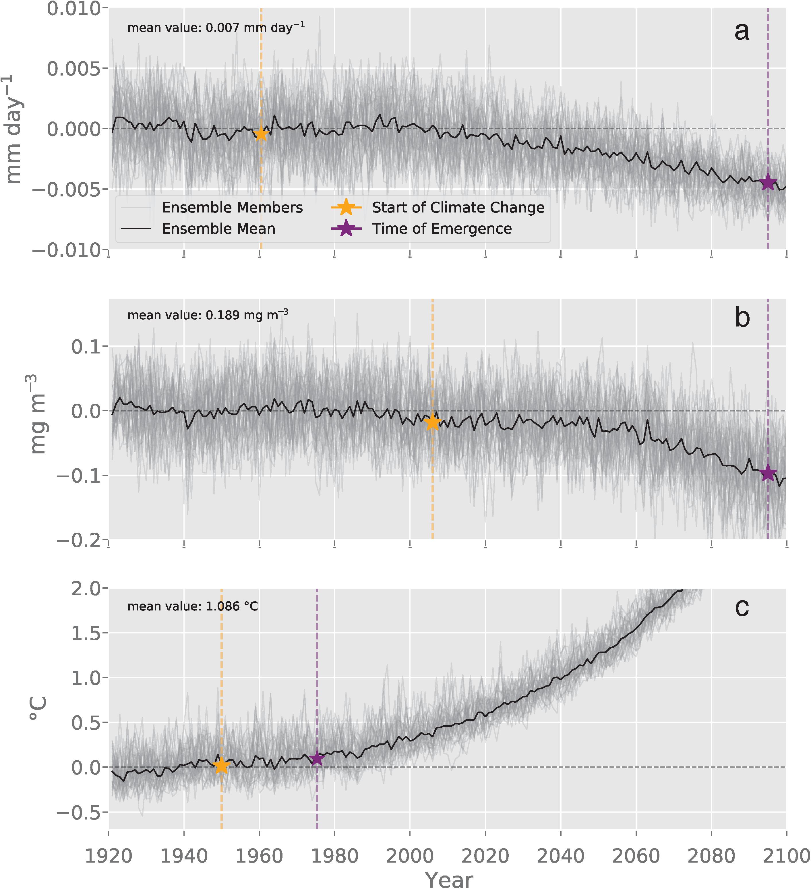
Figure 4. This plot of the spatially averaged modeled DJF fields for the Southern Ocean illustrates the temporal evolution of (a) krill growth potential anomaly (mm day^–1), (b) surface chlorophyll (mg m³), and (c) sea surface temperature (°C). Each ensemble member anomaly is plotted in gray while the black line is the mean ensemble anomaly. The means for each variable are listed in the upper left corner of each plot. The yellow stars indicate the year when the climate change signal was detected (Climate Change Year; GP: 1960, Chl: 2006, SST: 1950). The purple stars indicate the year of detection where trends forced by human-driven climate change can be formally distinguished from natural variability (Year of Detection; GP: 2095, Chl: 2095, SST: 1975) (Eq. 3).

The spatial patterns of natural variability were more pronounced at regional scales (Figure 3b) than across the spatial average of the Southern Ocean (Figure 4a). The general magnitude of natural variability across the spatial average of the krill GP anomaly was less than 0.005 mm day^–1m^–3 (Figure 4a). In contrast, the physical distribution of natural variability in krill GP was characterized by a widespread variability below 0.09 mm day^–1 with elevated variability along the coastal boundary of growth habitat. The physical distribution of natural variability in krill GP was characterized by areas of increased variability in the frontal zone of the ACC and near the tip of the eastern Antarctic Peninsula (Figure 3b). These areas coincided with higher amounts of variability in physical distribution of internal variability in chlorophyll (Figure 3f) where the internal variability of chlorophyll ranged up to an order of one higher than the mean state of 0.189 mg m^–3. Spatial patterns of variability in SST show higher variability around the boundary of the Polar Front and the eastern tip of Antarctic Peninsula (Figure 3j). Across temporal evolution of the spatial average of the anomaly, the magnitude of natural variability was less than 0.5°C (Figure 4c).

The trends in krill GP rates illustrate that the forced signal develops increasing dominance (over natural variability) at longer timescales. Spatial estimates of the contribution of natural variability on 20- and 50-year krill GP trends were computed by explicitly separating internal variability from the forced trend (Figure 5). Short- and long-term krill GP trends were calculated on the spatially resolved model output using a linear least-squares analysis beginning in 2020 and extending to 2040 and 2070, respectively. The forced trends computed over 20 and 50 years are broadly similar in their spatial patterns; the difference is primarily characterized by an intensification of the trend magnitude at the longer timescale and slightly more spatial coherence in the 50-year trend. Decomposing the 20- and 50-year total trends into internal variability and forced signal components illustrated the magnitude of natural variability within the system. Internal variability contributed modestly to 50-year trends but did not display recognizable spatial patterns (Figures 5g–l). In some regions, internal variability reinforced the 50-year forced trend, leading to greater rates of change, while in other regions, internal variability worked to oppose the forcing. Overall, 50-year trends in GP were dominated by the forced trend.

FIGURE 5

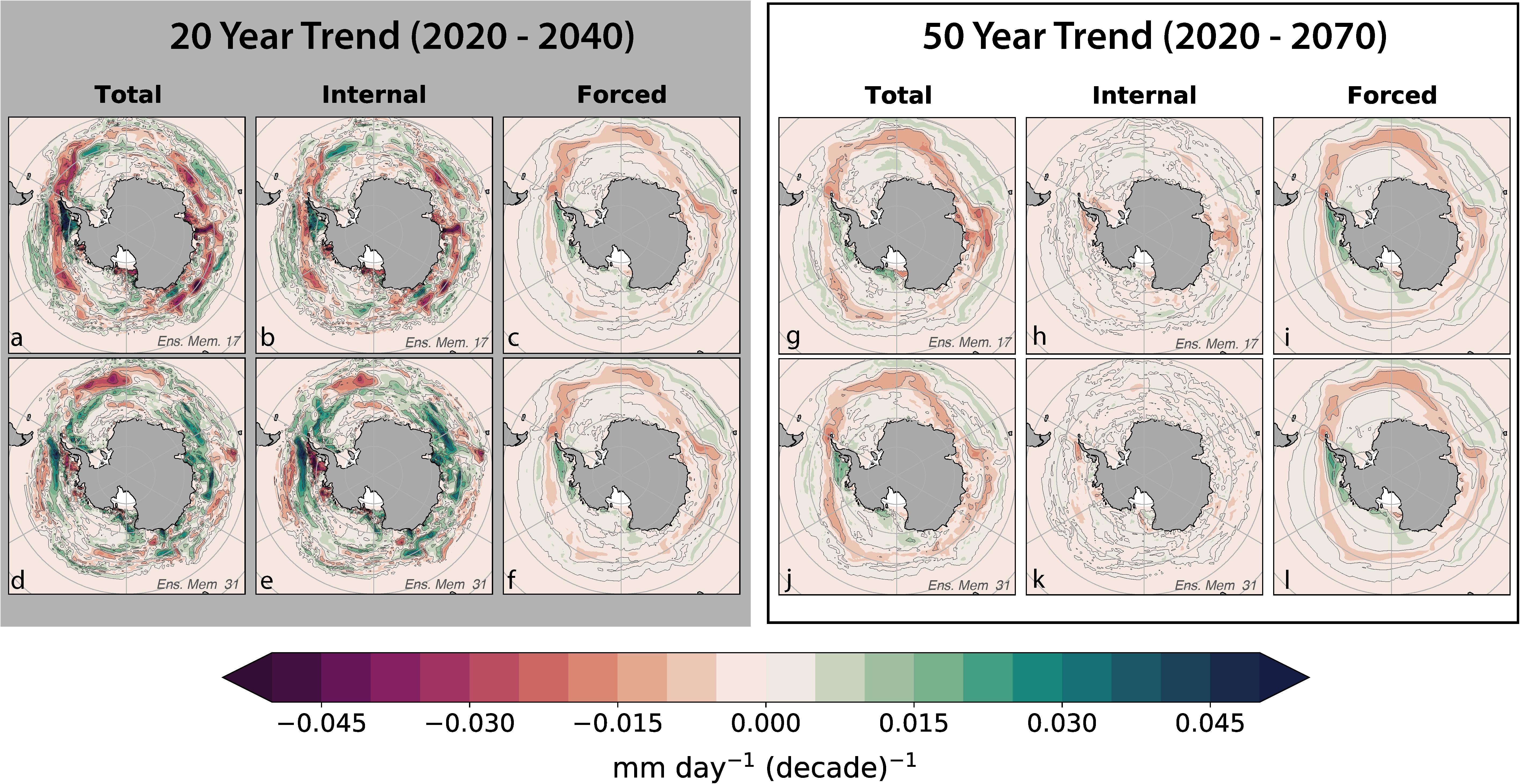
Figure 5. This figure demonstrates the superposition of forced signal and internal variability on the total 20- and 50-year trends of krill GP in austral summer beginning in 2020. Each row is from a separate ensemble member; the top row of plots (a–c and g–i) are from ensemble member 17 while the bottom row of plots (d–f and j–l) are from member number 31. These two ensemble members were chosen as exemplary representations from the ensemble. Plot (a,d) show the total linear trend in GP for the 20-year while plots (g,j) show the 50-year total linear trend. Plots (b,e) show the internal variability within the 20-year trend and plots (h,k) show the 50-year trend. The forced trend (ensemble mean) of the 20-year trend is shown in plot (c) and replicated in (f) and the 50-year forced trend is shown in plot (i) and replicated in (l). The forced trends are similar between both trend lengths but only drive the spatial coherence in the 50-year total trend, not the 20-year trend.

The ToE analysis revealed the presence and timing of when the forced signal became distinguishable from internal variability for each variable. The decline in the krill GP trend, due to the forced climate signal, became detectable at 2095 in the Southern Ocean, as did the trend in chlorophyll (Figures 4a,b). The earliest detection of the forced signal was observed in the SST anomaly, which became distinguishable from internal variability in 1975 across the Southern Ocean (Figure 4c).

Spatial distributions of ToE detection indicate that positive and negative regional trends were diagnosed as emergent late in the 21st century for krill GP. The regional forced trend of increased krill GP emerged near the Bellingshausen Sea, Amundsen Sea, and the eastern part of the Ross Sea (Figure 3e). Regional declines of the forced trend in krill GP emerged near the WAP and in the mid-Atlantic around the southern boundary of the ACC stretching west to the South Orkney Islands. By late in the 21 century, negative chlorophyll trends were diagnosed as emergent in the eastern Atlantic near the coast (Figures 3g,h). The region of emergent negative chlorophyll trends coincided with regions of early emergence of ocean warming trends. In comparison to GP and chlorophyll, the regional trends in SST emerged much earlier in the 21st century. The distribution was characterized by earlier emergence years in the eastern Atlantic and Indian quadrant (0° to 90°E) and coastal zones from the WAP and Bellingshausen Sea and around to the Ross Sea. There was no emergence in SST forced trends by 2100 from the eastern tip of the WAP to the South Sandwich Islands (Figure 3l). Areas where trends failed to emerge indicate that the ratio between the forced trend and natural variability was not significant enough to detect separate forced trends.

Discussion

Over the course of the CESM-LE simulation (1920–2100), krill GP rates are projected to decline during the summer season (Dec-Jan), a trend characterized by a poleward contraction of viable habitat (Figure 3c). The contraction of growth habitat is most noticeable around krill’s current population center from the South Sandwich Islands to the Antarctic Peninsula (Atkinson et al., 2008, 2019). This contraction is a consequence of warming ocean conditions in lower latitudes and the Antarctic Peninsula (Figure 3i) and krill’s sensitivity to temperature at the upper limits of their thermotolerance (Atkinson et al., 2006; Murphy et al., 2017). In our study, at higher latitudes the increase in forced trend of SST exposed habitat with high chlorophyll concentrations where krill growth had previously been inhibited due to low temperatures (>−1°C) (Figure 3). As a result, regional growth habitat increased in the Bellingshausen, Amundsen, and Ross Seas. These broad patterns of change in krill growth habitat in our results are reflected in similar studies using ESMs from the CMIP5 project. Within the Atlantic sector, Hill et al. (2013) found that krill growth habitat would be reduced based on ocean warming and reduced chlorophyll. Veytia et al. (2020) found that circumpolar growth habitat was projected to decline in the austral summer over the course of the century and contract toward higher latitudes. Their results, like ours, suggest that projected changes in chlorophyll and SST will reduce krill GP rates in low latitudes but will increase GP rates in higher latitudes.

Natural variability in krill growth habitat is influenced by changes in chlorophyll as well as temperature. Within the Atkinson et al. (2006) growth model, the relationship between growth and chlorophyll is highly nonlinear. Small changes in chlorophyll concentrations have a larger impact on the growth rate than temperatures within the stenothermic range because chlorophyll is the primary driver for krill growth potential and distribution (Ross et al., 2000; Atkinson et al., 2006; Murphy et al., 2017). This is illustrated in the temporal evolution of the spatial average in krill GP where the fluctuations in the magnitude of internal variability in krill are parallel with chlorophyll until early in the 21st century. Around 2020, the forced trend in krill GP and chlorophyll became more negative until the end of the century (Figures 4a,b). While this occurred, the magnitude of variability in krill GP was reduced but magnitude of variability of chlorophyll did not. Decreased variability in krill GP indicates when the forced trend could become dominant over natural variability. We hypothesize that as temperature contracts poleward, fluctuations in the position of the 5°C isotherm led to smaller perturbations in the total area of krill habitat, assuming that circumpolar habitat is well described by a regression with the area encompassed by the isotherm.

Trends associated with the forced signal are unlikely to be reversed on short timescales or can only be reversed through climate intervention strategies. Natural variability, however, implies fluctuations around a nominal mean state. Trends in krill GP are driven by the ratio of the magnitude of natural variability compared to the magnitude of the forced signal. These trends illustrate that the forced signal develops increasing dominance (over natural variability) at longer timescales (Figure 5). This is in line with the general understanding that the importance of natural variability is higher at smaller spatial and temporal scales (Hawkins and Sutton, 2012). Additionally, our results are consistent with other studies examining ToE that have found global emergence time scales of 20–30 year for SST and longer scales (50+ years) for surface chlorophyll (Schlunegger et al., 2020). This demonstrates that strong decadal variability is an important feature of the Southern Ocean ecosystem and is likely to dominate the evolution of the system at local to regional scales for the next few decades. From a management perspective, this approach could then be used to inform which climate signal to manage for, on what timescale, and what observational system would be needed to validate the projections.

Our ability to discern the influence of climate change is contingent upon the magnitude of the forced signal in relation to the magnitude of the natural variability. Across the Southern Ocean, the forced trend in krill GP emerges out of the envelope of natural variability late in the 21st century. The spatial patterns of ToE detection highlight the complexities of climate change on krill potential growth habitat: krill GP trends are both increasing and decreasing as a result of human driven climate change. By the mid to late 21st century, an increased krill GP trend emerged in habitat around the Bellingshausen/Amundsen Sea region (Figure 3). This result is again similar to projections by the 2016 study that found increased successful spawning habitats for krill in the late 21st century (Piñones and Fedorov, 2016). Currently the Bellingshausen and Amundsen Sea region does not support successful growth or spawning due to insufficient conditions (Piñones and Fedorov, 2016). However, the region has been characterized as habitat for potential future krill recruitment and increased population (Quetin and Ross, 2003) due to increased phytoplankton growth from increased ice-free summer days (Montes-Hugo et al., 2009). Though the GP model used in this study does not account for sea-ice, the spatial trend of increased SST in the Bellingshausen/Amundsen Sea region was diagnosed to emerge in SST by mid to late 21st century.

Declining krill GP rates in the habitat were detected by the late 21st century around the South Sandwich Islands, South Orkney Islands and the tip of the WAP. This region is part of the southwest Atlantic sector (30 to 70°W) of the Atlantic where 70% of the current population of krill is concentrated (Atkinson et al., 2008). Our results suggest that the decline in GP rates could coincide with emergent warming trends along the WAP. A similar projected decline in successful krill spawning habitat was found in the same region by a study using ESMs from the CMIP5 project and an early life cycle krill development model (Piñones and Fedorov, 2016). The 2016 study speculated that this decline was controlled by the significant changes in sea ice advance in the region north of Marguerite Bay (Piñones and Fedorov, 2016). The area around the WAP is considered to be the main seeding region for adult krill in the southwestern Atlantic (Hofmann et al., 1992; Fach et al., 2006; Thorpe et al., 2007, 2019). The significance of declining adult krill growth in the WAP suggests that human driven climate change will result in widespread negative effects on the krill dependent ecosystem. However, the forced changes in krill GP habitat are projected to be largely indistinguishable from natural variability until late the 21st-century.

Limitations

Along with the similarities in the spatial and temporal patterns in krill growth habitat between our results and previous studies using ESMs, there are slight variations in the spatial patterns and krill GP rates in our findings. These differences can be attributed to features of the underlying ESM simulations involved, as well as methodological details associated with the application of the krill model. The krill growth model used in this study was empirically derived using in situ and satellite data for adult krill growth in the summer season and represents a single growth-season. Additionally, the growth model does not properly account for the role of sea ice as it models growth in open ocean when sea ice is absent. Sea ice is thought to play a complex and crucial role in the krill life cycle, recruitment and abundance (Siegel and Loeb, 1995; Atkinson et al., 2004; Nicol, 2006; Thorpe et al., 2007; Piñones and Fedorov, 2016). However, there is minimal quantitative information regarding the relationship between sea ice and summer krill growth.

As an empirical model, the growth potential estimated is primarily descriptive and inherently limited in applicability by the conditions reflected in the dataset used in it’s formulation. Additionally, mechanistic knowledge gaps on krill population dynamics in response to environmental drivers currently preclude our ability to develop a model that can simulate the krill life cycle and obtain biomass estimates. Overall, these factors limit our ability to draw conclusions on actual krill biomass and production, but they do not significantly impede our ability to illustrate the projected spatial and temporal trends of climate change and natural variability in krill GP rates.

While our results are broadly consistent with previous studies, ours is the first to consider the effects of natural climate variability explicitly. Multi-model ensembles, like the CMIP5, are composed of multiple models, each with a distinct representation of the mean state and variability. Given the structural differences between the models, the multi-model ensemble cannot be easily used to explicitly separate natural variability and from forced trends (Solomon et al., 2011). However, the large-ensemble framework used in this study allows for quantification of the uncertainties from internal variability (as found in multi-model ensemble studies), identification of trends climate change and identifying when those trends can be formally distinguished from natural variability.

Because the krill model was applied to the model output offline, the resolution of the model output is limited in its ability to accurately project mean GP values at regional scales. For example, higher regional krill growth rates in some regions like the Bellingshausen Sea region may be partially due to the model’s bias for higher chlorophyll concentrations. However, the large ensemble framework assumptions result in a stronger ability to assess the trends and variability. As with any synthetic approach, limitations and caveats exist that stem from coarse model resolution, simplification of a complex system, or inadequate process representation. While these potential caveats are important to consider, they do not undermine our fundamental point regarding the critical role of both natural variability and external forcing in determining the trajectory of the system in coming decades.

Implications

Natural variability is, and will remain, a fundamental reality of the Southern Ocean. It will also remain a challenge for understanding of the ecosystem’s response to climate change. Even under perfect observing capabilities, the detection of climate-change signals is limited by the noise of natural variability. Therefore, quantifying the impacts of climate change on a key species like krill requires understanding and separating the influences of the superposition of natural variability and the forced trend. Though our study on krill GP is highly idealized, we found that climate driven trends in krill GP are detectable at basin scales, while strong natural variability challenges detection at local and shorter time scales. These results have several important implications regarding the challenge of detecting and attributing ecological changes to climate change and decision making.

Managing systems characterized by strong natural variability is challenging as the influence of natural variability in climate has the potential to mask or enhance long term trends in climate (Hawkins, 2011) that may be difficult to reverse once they emerge. By providing distinction between influence of natural variability and longer-term climate change trends on the Southern Ocean ecosystem and krill GP, the results and approach presented here can provide insight for informing management as consideration of multi-decadal timescales is imperative for determining if the forced signal is driving change (Hawkins, 2011). We have shown how the influence of natural variability and climate change on circumpolar krill GP depends on time scale. The influence of natural variability dominates the spread of uncertainty in spatial patterns of krill GP. However, longer timescales show that the influence of the forced trend on the contraction of positive krill GP habitat and mean growth potential rates will dominate over the influence of natural variability. This work suggests that in addition to the quantification of climate change impacts, management strategies must explicitly acknowledge that the ecosystem exhibits strong variability. For example, natural variability is likely to primarily impact patterns in krill GP over the next two decades. Natural variability can mask trends in climate that may be difficult to reverse once they emerge. This work suggests that in addition to the quantification of climate change impacts, management strategies must explicitly acknowledge that the Southern Ocean ecosystem exhibits strong variability.

Trends in krill growth potential rates have wide reaching implications for the Antarctic marine ecosystem and it’s management. Studies have shown that habitat’s ability to support the growth and maintenance of adult krill can be used to identify crucial areas for krill biomass production and high spawning potential (Hill et al., 2013; Murphy et al., 2017). Decreases in summer-time krill GP have negative implications for reproductive performance due to the exponential relationship between adult size and fecundity (Tarling and Johnson, 2006; Siegel and Watkins, 2016). Furthermore, while the poleward shift in growth habitat distribution may not have consequences for growth habitat, it is likely to be inadequate habitat for spawning (Hofmann and Hüsrevoğlu, 2003) or connecting subpopulations (Siegel, 2016). Cascading ecological impacts to the Antarctic marine ecosystem are exasperated by the additional pressure on krill from the fishery (Nicol et al., 2012). Fluctuations in krill productivity pose challenges for current definitions of sustainable catch. For example, seasonal changes in the length of krill are important for interpreting stock structure for fisheries management (Tarling et al., 2016). The changes as a result of climate change and variability in krill productivity and habitat partitioning could cause major consequences for food web linkages, biogeochemical cycling (Cavan et al., 2019), and the krill fishery.

There is wide international recognition of the importance of understanding, and managing for, the impacts of climate variability and climate change on the Antarctic marine ecosystem (Brasier et al., 2019). We believe that the research presented here motivates questions regarding current management priorities. One of the current priorities of the Southern Ocean management body is developing a risk assessment framework to inform the spatial allocation of krill catch (CCAMLR, 2019, para 5.17). The framework development is a part of a long-term ecosystem-based management system for the Antarctic krill fishery. Based on our results, important fluctuations in krill dynamics are likely even in the absence of human-driven warming. If the management strategy envisioned for krill is based on short-term projections, data layers should include the spread of natural variability. When considering long-term projections, the risk assessment could also include one or more layers characterizing long-term outcomes. Consideration of long-term impacts could enhance the management strategy to be more robust or adaptive to the impacts of climate change.

While our approach has oversimplified the complexity involved with sustaining krill populations, the notion of coupling mechanistic ecosystem models to ESMs could provide a more reliable basis for adaptation strategies, risk analyses, and understanding trade-offs associated with climate change mitigation (Stock et al., 2011; Park et al., 2019). Achieving such an outcome would require coupling the ESM to a krill model that simulates life history dynamics and constraints on growth recruitment and mortality. Nature holds vastly more degrees of freedom than represented in our model and there is significant potential for other mechanisms to arise that fundamentally change the nature of the system’s response. A first step in that direction would be to adapt more advanced krill models like Constable and Kawaguchi’s model that simulates bioenergetics (Constable and Kawaguchi, 2018). The advancement of this approach will generate new methods for quantifying the impacts of climate change on the Antarctic marine ecosystem. For example, by virtue of the ability to separate the component of change due to natural variability from that associated with the forced trend, the separation enables a theoretical, yet direct, attribution of losses in krill production and yield to climate change (Bonan and Doney, 2018). In turn, these types of attributions could then be used to quantify the cost-benefit of climate mitigation and used to inform long term goals for a flexible management strategy.

Conclusion

The Southern Ocean is a dynamic system and appropriate consideration of the changes projected to accompany climate warming must recognize the important role of natural variability. The research presented here exemplifies a particular application of ESMs, targeted at exploring the specific climate drivers of changes in krill growth potential habitat. Our findings highlight the complexities of the detection and attribution of human-driven climate changes that are superimposed on changes occurring naturally as a result of chaotic dynamics in the climate system. In the context of understanding ecosystem dynamics in the Southern Ocean, the superposition of natural climate variability of force trends is a critical consideration. The basic conclusions of this study are as follows. We have demonstrated how a large ensemble framework can enable explicit assessments of the benefits of climate mitigation to krill habitat and provide perspectives relevant informing for management decisions on timescales ranging from seasons to centuries. We have shown that changes in krill growth potential will be driven by the superposition of natural variability on shorter timescales (≤20 years) but on longer timescales (≥50 years), changes will be driven by the forced trend. Furthermore, we have shown that it will be impossible to distinguish the forced signal from natural variability until deep into the 21st century in krill growth potential. These findings emphasize the need for proactive consideration of natural variability in Southern Ocean management of krill as it can mask trends in climate that may be difficult to reverse once they emerge. Future application of the large ensemble framework can be used to develop projections of krill habitat change inclusive of appropriate uncertainty estimates. In conclusion, both natural variability and externally forced trends will be important determinants of krill habitat over the coming decades. Studies such as this will be relevant and necessary for creating climate-informed management in a marine ecosystem of immense economic and intrinsic value.

Data Availability Statement

The raw data supporting the conclusions of this article will be made available by the authors, without undue reservation.

Author Contributions

All authors listed have made a substantial, direct and intellectual contribution to the work, and approved it for publication.

Funding

CB and ZS were supported by the Pew Charitable Trusts. ML was supported by NASA grant 19-IDS19-0028.

Conflict of Interest

The authors declare that the research was conducted in the absence of any commercial or financial relationships that could be construed as a potential conflict of interest.

Acknowledgments

Supercomputing, analysis, and storage resources were provided by the Computational and Information System Lab at the National Center for Atmospheric Research. We acknowledge high-performance computing support from Yellowstone (ark:/85065/d7wd3xhc) and Cheyenne (doi: 10.5065/D6RX99H) provided by NCAR’s Computational and Information Systems Laboratory. The National Center for Atmospheric Research is sponsored by the National Science Foundation. Thanks to Daniel Doak and Nicole Lovenduski for their valuable support and feedback on the manuscript. Thanks also to Anton Van de Putte for providing valuable opportunities to share this work and for his feedback throughout the process. We would also like to thank the reviewers and editor for their time, writing support, and constructive feedback. Lastly, thank you to the CCAMLR Secretariat, Members States and Observers for allowing authors to participate in their meetings. Data from the CESM Large Ensemble publicly available; multiple options for access are described here: https://www.cesm.ucar.edu/projects/community-projects/LENS/data-sets.html.

References

Allison, L. C., Johnson, H. L., Marshall, D. P., and Munday, D. R. (2010). Where do winds drive the Antarctic circumpolar current? Geophys. Res. Lett. 37:L12605. doi: 10.1029/2010GL043355

CrossRef Full Text | Google Scholar

Atkinson, A., Hill, S. L., Pakhomov, E. A., Siegel, V., Reiss, C. S., Loeb, V. J., et al. (2019). Krill (Euphausia superba) distribution contracts southward during rapid regional warming. Nat. Clim. Chang. 9, 142–147. doi: 10.1038/s41558-018-0370-z

CrossRef Full Text | Google Scholar

Atkinson, A., Shreeve, R. S., Hirst, A. G., Rothery, P., Tarling, G. A., Pond, D. W., et al. (2006). Natural growth rates in Antarctic krill (Euphausia superba): II. Predictive models based on food, temperature, body length, sex, and maturity stage. Limnol. Oceanogr. 51, 973–987. doi: 10.4319/lo.2006.51.2.0973

CrossRef Full Text | Google Scholar

Atkinson, A., Siegel, V., Pakhomov, E., and Rothery, P. (2004). Long-term decline in krill stock and increase in salps within the Southern Ocean. Nature 432, 100–103. doi: 10.1038/nature02996

PubMed Abstract | CrossRef Full Text | Google Scholar

Atkinson, A., Siegel, V., Pakhomov, E., Rothery, P., Loeb, V., Ross, R., et al. (2008). Oceanic circumpolar habitats of Antarctic krill. Mar. Ecol. Prog. Ser. 362, 1–23. doi: 10.3354/meps07498

CrossRef Full Text | Google Scholar

Atkinson, A., Siegel, V., Pakhomov, E. A., Jessopp, M. J., and Loeb, V. (2009). A re-appraisal of the total biomass and annual production of Antarctic krill. Deep Sea Res. 1 Oceanogr. Res. Pap. 56, 727–740. doi: 10.1016/j.dsr.2008.12.007

CrossRef Full Text | Google Scholar

Bonan, G. B., and Doney, S. C. (2018). Climate, ecosystems, and planetary futures: the challenge to predict life in Earth system models. Science 359:eaam8328. doi: 10.1126/science.aam8328

PubMed Abstract | CrossRef Full Text | Google Scholar

Bopp, L., Resplandy, L., Orr, J. C., Doney, S. C., Dunne, J. P., Gehlen, M., et al. (2013). Multiple stressors of ocean ecosystems in the 21st century: projections with CMIP5 models. Biogeosciences 10, 6225–6245. doi: 10.5194/bg-10-6225-2013

CrossRef Full Text | Google Scholar

Brady, R. X., Alexander, M. A., Lovenduski, N. S., and Rykaczewski, R. R. (2017). Emergent anthropogenic trends in California current upwelling. Geophys. Res. Lett. 44, 5044–5052. doi: 10.1002/2017gl072945

CrossRef Full Text | Google Scholar

Brasier, M. J., Constable, A., Melbourne-Thomas, J., Trebilco, R., Griffiths, H., Van de Putte, A., et al. (2019). Observations and models to support the first Marine Ecosystem Assessment for the Southern Ocean (MEASO). J. Mar. Sys. 197:103182. doi: 10.1016/j.jmarsys.2019.05.008

CrossRef Full Text | Google Scholar

Cavan, E. L., Belcher, A., Atkinson, A., Hill, S. L., Kawaguchi, S., McCormack, S., et al. (2019). The importance of Antarctic krill in biogeochemical cycles. Nat. Commun. 10, 1–13.

Google Scholar

CCAMLR (2019). Report of the XXXVIII Meeting of the Commission. Hobart, Tas: Commission for the Conservation of Antarctic Marine Living Resources.

Google Scholar

Commission on Geosciences, Environment, and Resources, Climate Research Committee, National Research Council, and Division on Earth and Life Studies (1996). Natural Climate Variability on Decade-To-Century Time Scales. Washington, DC: National Academies Press.

Google Scholar

Constable, A. (2000). Managing fisheries to conserve the Antarctic marine ecosystem: practical implementation of the Convention on the Conservation of Antarctic Marine Living Resources (CCAMLR). ICES J. Mar. Sci. 57, 778–791. doi: 10.1006/jmsc.2000.0725

CrossRef Full Text | Google Scholar

Constable, A. J., and Kawaguchi, S. (2018). Modelling growth and reproduction of Antarctic krill, Euphausia superba, based on temperature, food and resource allocation amongst life history functions. ICES J. Mar. Sci. 75, 738–750. doi: 10.1093/icesjms/fsx190

CrossRef Full Text | Google Scholar

Constable, A. J., Melbourne−Thomas, J., Corney, S. P., Arrigo, K. R., Barbraud, C., Barnes, D. K. A., et al. (2014). Climate change and southern Ocean ecosystems I: how changes in physical habitats directly affect marine biota. Glob. Chang. Biol. 20, 3004–3025.

Google Scholar

Danabasoglu, G., Bates, S. C., Briegleb, B. P., Jayne, S. R., Jochum, M., Large, W. G., et al. (2012). The CCSM4 ocean component. J. Clim. 25, 1361–1389. doi: 10.1175/jcli-d-11-00091.1

CrossRef Full Text | Google Scholar

Deser, C., Phillips, A., Bourdette, V., and Teng, H. (2012). Uncertainty in climate change projections: the role of internal variability. Clim. Dyn. 38, 527–546. doi: 10.1007/s00382-010-0977-x

CrossRef Full Text | Google Scholar

Doney, S. C., Ruckelshaus, M., Emmett Duffy, J., Barry, J. P., Chan, F., English, C. A., et al. (2012). Climate change impacts on marine ecosystems. Annu. Rev. Mar. Sci. 4, 11–37.

Google Scholar

Fach, B., Hofmann, E., and Murphy, E. (2002). Modeling studies of Antarctic krill Euphausia superba survival during transport across the Scotia Sea. Mar. Ecol. 231, 187–203. doi: 10.3354/meps231187

CrossRef Full Text | Google Scholar

Fach, B. A., Hofmann, E. E., and Murphy, E. J. (2006). Transport of Antarctic krill (Euphausia superba) across the Scotia Sea. Part II: krill growth and survival. Deep Sea Res. 1 Oceanogr. Res. Pap. 53, 1011–1043. doi: 10.1016/j.dsr.2006.03.007

CrossRef Full Text | Google Scholar

Feldstein, S. B. (2000). The timescale, power spectra, and climate noise properties of teleconnection patterns. J. Clim. 13, 4430–4440. doi: 10.1175/1520-0442(2000)013<4430:ttpsac>2.0.co;2

CrossRef Full Text | Google Scholar

Flores, H., Atkinson, A., Kawaguchi, S., Krafft, B., Milinevsky, G., Nicol, S., et al. (2012). Impact of climate change on Antarctic krill. Mar. Ecol. Prog. Ser. 458, 1–19.

Google Scholar

Fogt, R. L., and Marshall, G. J. (2020). The southern annular mode: variability, trends, and climate impacts across the southern hemisphere. WIREs Clim. Chang. 11:e652.

Google Scholar

Goyal, R., Gupta, A. S., Jucker, M., and England, M. H. (2021). Historical and projected changes in the southern hemisphere surface westerlies. Geophys. Res. Lett. 48:e2020GL090849.

Google Scholar

Hadley Centre for Climate Prediction and Research (2000). Hadley Centre Global Sea Ice and Sea Surface Temperature (HadISST). doi: 10.5065/XMYE-AN84

CrossRef Full Text | Google Scholar

Hagen, J. O., Jefferies, R., Marchant, H., Nelson, F., Prowse, T., Vaughan, D. G., et al. (2007). Polar Regions (Arctic and Antarctic). Cambridge University Press, Contribution of Working Group II: Impacts, Adaptation and Vulnerability Fourth Assessment Report of the Intergovernmental Panel on Climate Change. Cambridge: Cambridge University Press.

Google Scholar

Hasselmann, K. (1976). Stochastic climate models part I. Theory. Tellus 28, 473–485. doi: 10.1111/j.2153-3490.1976.tb00696.x

CrossRef Full Text | Google Scholar

Hasselmann, K. (1993). Optimal fingerprints for the detection of time-dependent climate change. J. Clim. 6, 1957–1971. doi: 10.1175/1520-0442(1993)006<1957:offtdo>2.0.co;2

CrossRef Full Text | Google Scholar

Hawkins, E. (2011). Our evolving climate: communicating the effects of climate variability. Weather 66, 175–179. doi: 10.1002/wea.761

CrossRef Full Text | Google Scholar

Hawkins, E., and Sutton, R. (2009). The potential to narrow uncertainty in regional climate predictions. Bull. Am. Meteorol. Soc. 90, 1095–1108. doi: 10.1175/2009bams2607.1

CrossRef Full Text | Google Scholar

Hawkins, E., and Sutton, R. (2012). Time of emergence of climate signals. Geophys. Res. Lett. 39, L01702. doi: 10.1029/2011GL050087

CrossRef Full Text | Google Scholar

Henley, S. F., Schofield, O. M., Hendry, K. R., Schloss, I. R., Steinberg, D. K., Moffat, C., et al. (2019). Variability and change in the west Antarctic Peninsula marine system: research priorities and opportunities. Prog. Oceanogr. 173, 208–237.

Google Scholar

Henson, S. A., Beaulieu, C., Ilyina, T., John, J. G., Long, M., Séférian, R., et al. (2017). Rapid emergence of climate change in environmental drivers of marine ecosystems. Nat. Commun. 8:14682.

Google Scholar

Hill, S. L., Phillips, T., and Atkinson, A. (2013). Potential climate change effects on the habitat of Antarctic krill in the weddell quadrant of the southern ocean. PLoS One 8:e72246. doi: 10.1371/journal.pone.0072246

PubMed Abstract | CrossRef Full Text | Google Scholar

Hobbs, W. R., Massom, R., Stammerjohn, S., Reid, P., Williams, G., and Meier, W. (2016). A review of recent changes in Southern Ocean sea ice, their drivers and forcings. Glob. Planet. Chang. 143, 228–250. doi: 10.1016/j.gloplacha.2016.06.008

CrossRef Full Text | Google Scholar

Hofmann, E., Capella, J. E., Ross, R. M., and Quetin, L. B. (1992). Models of the early life history of Euphausia superba—Part I. Time and temperature dependence during the descent-ascent cycle. Deep Sea Res. A Oceanogr. Res. Pap. 39, 1177–1200. doi: 10.1016/0198-0149(92)90063-y

CrossRef Full Text | Google Scholar

Hofmann, E., and Hüsrevoğlu, Y. (2003). A circumpolar modeling study of habitat control of Antarctic krill (Euphausia superba) reproductive success. Deep Sea Res. 2 Top. Stud. Oceanogr. 50, 3121–3142. doi: 10.1016/j.dsr2.2003.07.012

CrossRef Full Text | Google Scholar

Hofmann, E., and Lascara, C. (2000). Modeling the growth dynamics of Antarctic krill Euphausia superba. Mar. Ecol. Prog. Ser. 194, 219–231. doi: 10.3354/meps194219

CrossRef Full Text | Google Scholar

Holland, M. M., Bailey, D. A., Briegleb, B. P., Light, B., and Hunke, E. (2012). Improved sea ice shortwave radiation physics in CCSM4: the impact of melt ponds and aerosols on arctic sea ice. J. Clim. 25, 1413–1430. doi: 10.1175/jcli-d-11-00078.1

CrossRef Full Text | Google Scholar

Hunke, E. C., and Lipscomb, W. H. (2010). CICE: The Los Alamos Sea Ice Model Documentation and Software User’s Manual Version 4. Los Alamos, NM: Los Alamos National Lab. (LANL), 76.

Google Scholar

Hurrell, J. W., Holland, M. M., Gent, P. R., Ghan, S., Kay, J. E., Kushner, P. J., et al. (2013). The community earth system model: a framework for collaborative research. Bull. Am. Meteorol. Soc. 94, 1339–1360.

Google Scholar

Kay, J. E., Deser, C., Phillips, A. S., Mai, A., Hannay, C., Strand, G., et al. (2015). The community earth system model (CESM) large ensemble project: a community resource for studying climate change in the presence of internal climate variability. Bull. Am. Meteorol. Soc. 96, 1333–1349. doi: 10.1175/bams-d-13-00255.1

CrossRef Full Text | Google Scholar

Larsen, J. N., Anisimov, O. A., Constable, A., Hollowed, A. B., Maynard, N., Prestrud, P., et al. (2014). Polar Regions, in: Climate Change 2014–Impacts, Adaptation and Vulnerability: Part B: Regional Aspects: Working Group II Contribution to the IPCC Fifth Assessment Report. Cambridge: Cambridge University Press, 1567–1612.

Google Scholar

Lawrence, D. M., Oleson, K. W., Flanner, M. G., Fletcher, C. G., Lawrence, P. J., Levis, S., et al. (2012). The CCSM4 land simulation, 1850–2005: assessment of surface climate and new capabilities. J. Clim. 25, 2240–2260. doi: 10.1175/jclid-11-00103.1

CrossRef Full Text | Google Scholar

Le Quéré, C., Buitenhuis, E. T., Moriarty, R., Alvain, S., Aumont, O., Bopp, L., et al. (2016). Role of zooplankton dynamics for southern ocean phytoplankton biomass andglobal biogeochemical cycles. Biogeosciences 13, 4111–4133. doi: 10.5194/bg-13-4111-2016

CrossRef Full Text | Google Scholar

Long, M. C., Deutsch, C., and Ito, T. (2016). Finding forced trends in oceanic oxygen. Glob. Biogeochem. Cycles 30, 381–397. doi: 10.1002/2015gb005310

CrossRef Full Text | Google Scholar

Lovenduski, N. S., McKinley, G. A., Fay, A. R., Lindsay, K., and Long, M. C. (2016). Partitioning uncertainty in ocean carbon uptake projections: internal variability, emission scenario, and model structure. Glob. Biogeochem. Cycles 30, 1276–1287. doi: 10.1002/2016gb005426

CrossRef Full Text | Google Scholar

Mayewski, P. A., Meredith, M. P., Summerhayes, C. P., Turner, J., Worby, A., Barrett, P. J., et al. (2009). State of the Antarctic and southern ocean climate system. Rev. Geophys. 47:RG1003.

Google Scholar

McBride, M. M., Dalpadado, P., Drinkwater, K. F., Godø, O. R., Hobday, A. J., Hollowed, A. B., et al. (2014). Krill, climate, and contrasting future scenarios for Arctic and Antarctic fisheries. ICES J. Mar. Sci. 71, 1934–1955. doi: 10.1093/icesjms/fsu002

CrossRef Full Text | Google Scholar

Meyer, B., Atkinson, A., Bernard, K. S., Brierley, A. S., Driscoll, R., Hill, S. L., et al. (2020). Successful ecosystem-based management of Antarctic krill should address uncertainties in krill recruitment, behaviour and ecological adaptation. Commun. Earth Environ. 1, 1–12.

Google Scholar

Montes-Hugo, M., Doney, S. C., Ducklow, H. W., Fraser, W., Martinson, D., Stammerjohn, S. E., et al. (2009). Recent changes in phytoplankton communities associated with rapid regional climate change along the western Antarctic Peninsula. Science 323, 1470–1473. doi: 10.1126/science.1164533

PubMed Abstract | CrossRef Full Text | Google Scholar

Murphy, E. J., Cavanagh, R. D., Hofmann, E. E., Hill, S. L., Constable, A. J., Costa, D. P., et al. (2012). Developing integrated models of Southern Ocean food webs: including ecological complexity, accounting for uncertainty and the importance of scale. Prog. Oceanogr. End End Model. Toward Comp. Anal. Mar. Ecosyst. Org. 102, 74–92. doi: 10.1016/j.pocean.2012.03.006

CrossRef Full Text | Google Scholar

Murphy, E. J., Thorpe, S. E., Tarling, G. A., Watkins, J. L., Fielding, S., and Underwood, P. (2017). Restricted regions of enhanced growth of Antarctic krill in the circumpolar Southern Ocean. Sci. Rep. 7:6963.

Google Scholar

NASA Ocean Biology Processing Group (2018). SEAWIFS-ORBVIEW-2 Level 3 Binned Chlorophyll Data Version R2018.0. Greenbelt, MD: NASA Ocean Biology Processing Group, doi: 10.5067/ORBVIEW-2/SEAWIFS/L3B/CHL/2018

CrossRef Full Text | Google Scholar

Nicol, S. (2006). Krill, currents, and sea ice: Euphausia superba and its changing environment. BioScience 56, 111–120. doi: 10.1641/0006-3568(2006)056[0111:kcasie]2.0.co;2

CrossRef Full Text | Google Scholar

Nicol, S., and Foster, J. (2016). “The fishery for antarctic krill: its current status and management regime,” in Biology and Ecology of Antarctic Krill, Advances in Polar Ecology, ed. V. Siegel (Cham: Springer International Publishing), 387–421.

Google Scholar

Nicol, S., Foster, J., and Kawaguchi, S. (2012). The fishery for Antarctic krill–recent developments: krill fishery review. Fish Fish. 13, 30–40. doi: 10.1111/j.1467-2979.2011.00406.x

CrossRef Full Text | Google Scholar

Nicol, S., and Mangel, M. (2018). The Curious Life of Krill: A Conservation Story from the Bottom of the World. Washington, DC: Island Press.

Google Scholar

Orsi, A. H., Whitworth, T., and Nowlin, W. D. (1995). On the meridional extent and fronts of the Antarctic 802 Circumpolar Current. Deep Sea Res. Part I: Oceanogr. Res. Pap. 42, 641–673. doi: 10.1016/0967-0637(95)00021-W

CrossRef Full Text | Google Scholar

Park, J.-Y., Stock, C. A., Dunne, J. P., Yang, X., and Rosati, A. (2019). Seasonal to multiannual marine ecosystem prediction with a global Earth system model. Science 365, 284–288. doi: 10.1126/science.aav6634

PubMed Abstract | CrossRef Full Text | Google Scholar

Piñones, A., and Fedorov, A. V. (2016). Projected changes of Antarctic krill habitat by the end of the 21st century: changes in Antarctic krill habitat. Geophys. Res. Lett. 43, 8580–8589. doi: 10.1002/2016gl069656

CrossRef Full Text | Google Scholar

Quéré, C. L., Harrison, S. P., Prentice, I. C., Buitenhuis, E. T., Aumont, O., Bopp, L., et al. (2005). Ecosystem dynamics based on plankton functional types for global ocean biogeochemistry models. Glob. Chang. Biol. 11, 2016–2040.

Google Scholar

Quetin, L., and Ross, R. (2003). Episodic recruitment in Antarctic krill Euphausia superba in the Palmer LTER study region. Mar. Ecol. Prog. Ser. 259, 185–200. doi: 10.3354/meps259185

CrossRef Full Text | Google Scholar

Rogers, A. D., Frinault, B. A. V., Barnes, D. K. A., Bindoff, N. L., Downie, R., Ducklow, H. W., et al. (2020). Antarctic futures: an assessment of climate-driven changes in ecosystem structure, function, and service provisioning in the Southern Ocean. Annu. Rev. Mar. Sci. 12, 87–120. doi: 10.1146/annurev-marine-010419-011028

PubMed Abstract | CrossRef Full Text | Google Scholar

Rogers, J. C., and van Loon, H. (1982). Spatial variability of sea level pressure and 500 mb height anomalies over the southern hemisphere. Mon. Weather Rev. 110, 1375–1392. doi: 10.1175/1520-0493(1982)110<1375:svoslp>2.0.co;2

CrossRef Full Text | Google Scholar

Ross, R. M., Quetin, L. B., Baker, K. S., Vernet, M., and Smith, R. C. (2000). Growth limitation in young Euphausia superba under field conditions. Limnol. Oceanogr. 45, 31–43. doi: 10.4319/lo.2000.45.1.0031

CrossRef Full Text | Google Scholar

Ryabov, A. B., de Roos, A. M., Meyer, B., Kawaguchi, S., and Blasius, B. (2017). Competition-induced starvation drives large-scale population cycles in Antarctic krill. Nat. Ecol. Evol. 1:0177.

Google Scholar

Santer, B. D., Mears, C., Doutriaux, C., Caldwell, P., Gleckler, P. J., Wigley, T. M. L., et al. (2011). Separating signal and noise in atmospheric temperature changes: the importance of timescale. J. Geophys. Res. Atmos. 116:D22105. doi: 10.1029/2011JD016263

CrossRef Full Text | Google Scholar

Schlunegger, S., Rodgers, K. B., Sarmiento, J. L., Ilyina, T., Dunne, J. P., Takano, Y., et al. (2020). Time of emergence and large ensemble intercomparison for ocean biogeochemical trends. Glob. Biogeochem. Cycles 34:e2019GB006453.

Google Scholar

Schmidt, K., Atkinson, A., Steigenberger, S., Fielding, S., Lindsay, M. C. M., Pond, D. W., et al. (2011). Seabed foraging by Antarctic krill: implications for stock assessment, bentho-pelagic coupling, and the vertical transfer of iron. Limnol. Oceanogr. 56, 1411–1428. doi: 10.4319/lo.2011.56.4.1411

CrossRef Full Text | Google Scholar

Siegel, V. (Ed). (2016). Biology and Ecology of Antarctic krill, Advances in Polar Ecology. Cham: Springer International Publishing, doi: 10.1007/978-3-319-29279-3

CrossRef Full Text | Google Scholar

Siegel, V., and Loeb, V. (1995). Recruitment of Antarctic krill Euphausia superba and possible causes for its variability. Mar. Ecol. Prog. Ser. 123, 45–56. doi: 10.3354/meps123045

CrossRef Full Text | Google Scholar

Siegel, V., and Watkins, J. L. (2016). “Distribution, Biomass and Demography of Antarctic krill, Euphausia superba,” in Biology and Ecology of Antarctic Krill, Advances in Polar Ecology, ed. V. Siegel (Cham: Springer International Publishing), 21–100. doi: 10.1007/978-3-319-29279-3_2

CrossRef Full Text | Google Scholar

Solomon, A., Goddard, L., Kumar, A., Carton, J., Deser, C., Fukumori, I., et al. (2011). Distinguishing the roles of natural and anthropogenically forced decadal climate variability: implications for prediction. Bull. Am. Meteorol. Soc. 92, 141–156. doi: 10.1175/2010bams2962.1

CrossRef Full Text | Google Scholar

Stammerjohn, S., Massom, R., Rind, D., and Martinson, D. (2012). Regions of rapid sea ice change: an inter-hemispheric seasonal comparison. Geophys. Res. Lett. 39:L06501. doi: 10.1029/2012GL050874

CrossRef Full Text | Google Scholar

Stammerjohn, S. E., and Maksym, T. (2017). “Gaining (and losing) Antarctic sea ice: variability, trends and mechanisms,” in Sea Ice, ed. D. N. Thomas (Oxford: Wiley-Blackwell), 261–289. doi: 10.1002/9781118778371.ch10

CrossRef Full Text | Google Scholar

Stock, C. A., Alexander, M. A., Bond, N. A., Brander, K. M., Cheung, W. W. L., Curchitser, E. N., et al. (2011). On the use of IPCC-class models to assess the impact of climate on living marine resources. Prog. Oceanogr. 88, 1–27. doi: 10.1016/j.pocean.2010.09.001

CrossRef Full Text | Google Scholar

Tarling, G., Hill, S., Peat, H., Fielding, S., Reiss, C., and Atkinson, A. (2016). Growth and shrinkage in Antarctic krill Euphausia superba is sex-dependent. Mar. Ecol. Prog. Ser. 547, 61–78. doi: 10.3354/meps11634

CrossRef Full Text | Google Scholar

Tarling, G. A., and Fielding, S. (2016). “Swarming and Behaviour in Antarctic krill,” in Biology and Ecology of Antarctic Krill, Advances in Polar Ecology, ed. V. Siegel (Cham: Springer International Publishing), 279–319. doi: 10.1007/978-3-319-29279-3_8

CrossRef Full Text | Google Scholar

Tarling, G. A., and Johnson, M. L. (2006). Satiation gives krill that sinking feeling. Curr. Biol. 16, R83–R84.

Google Scholar

Thompson, D. W. J., and Wallace, J. M. (2000). Annular modes in the extratropical circulation. Part I: month-to-month variability. J. Clim. 13:17.

Google Scholar

Thorpe, S., Tarling, G., and Murphy, E. (2019). Circumpolar patterns in Antarctic krill larval recruitment: an environmentally driven model. Mar. Ecol. Prog. Ser. 613, 77–96. doi: 10.3354/meps12887

CrossRef Full Text | Google Scholar

Thorpe, S. E., Murphy, E. J., and Watkins, J. L. (2007). Circumpolar connections between Antarctic krill (Euphausia superba Dana) populations: investigating the roles of ocean and sea ice transport. Deep Sea Res. 1 Oceanogr. Res. Pap. 54, 792–810. doi: 10.1016/j.dsr.2007.01.008

CrossRef Full Text | Google Scholar

Tommasi, D., Stock, C. A., Hobday, A. J., Methot, R., Kaplan, I. C., Eveson, J. P., et al. (2017). Managing living marine resources in a dynamic environment: the role of seasonal to decadal climate forecasts. Prog. Oceanogr. 152, 15–49.

Google Scholar

Trathan, P. N., and Hill, S. L. (2016). “The Importance of krill Predation in the Southern Ocean,” in Biology and Ecology of Antarctic Krill, Advances in Polar Ecology, ed. V. Siegel (Cham: Springer International Publishing), 321–350. doi: 10.1007/978-3-319-29279-3_9

CrossRef Full Text | Google Scholar

Turner, J., Lu, H., White, I., King, J. C., Phillips, T., Hosking, J. S., et al. (2016). Absence of 21st century warming on Antarctic Peninsula consistent with natural variability. Nature 535, 411–415. doi: 10.1038/nature18645

PubMed Abstract | CrossRef Full Text | Google Scholar

Veytia, D., Corney, S., Meiners, K. M., Kawaguchi, S., Murphy, E. J., and Bestley, S. (2020). Circumpolar projections of Antarctic krill growth potential. Nat. Clim. Chang. 10, 568–575. doi: 10.1038/s41558-020-0758-4

CrossRef Full Text | Google Scholar

Watters, G. M., Hinke, J. T., and Reiss, C. S. (2020). Long-term observations from Antarctica demonstrate that mismatched scales of fisheries management and predator-prey interaction lead to erroneous conclusions about precaution. Sci. Rep. 10:2314.

Google Scholar