ConvLSTM-Based Wave Forecasts in the South and East China Seas

Introduction

Ocean surface gravity waves (hereinafter, waves) are strongly non-linear and significantly affect ocean engineering activities, maritime operations, and transportation. Traditional wave forecasting models have been continuously developed and improved. Currently, the most widely used models are the WaveWatch III (WW3) by the US National Centers for Environmental Prediction, the Simulating Waves Nearshore (SWAN) by the Netherlands Delft University, and so on. The traditional numerical wave models are based on the wave action balance equation and adopt gridded discretization instead of differential equations. This inevitably introduces numerical errors and faces problems such as non-convergence and instability in numerical computations. Additionally, numerical models are highly sensitive to the simulated area terrain (especially in shallow nearshore waters) and computational domain boundaries. They also require input information of many other variables, such as wind data (Niu and Feng, 2021). Uncertainties of these external variables lead to additional model errors, which further affect the model’s accuracy. Numerical models also consume large amounts of computational resources and need to run for long periods of time, which is often impractical in emergency situations and thus is a significant bottleneck that restricts the development of fast and accurate wave forecasts.

With the rapid development of artificial intelligence (AI), due to its applicability across diverse fields and the ability to consider non-linearities in complex physical mechanisms, AI techniques have been widely applied in the field of marine sciences. These range from the automatic detection and prediction of mesoscale eddies (Zeng et al., 2015; Xu et al., 2019), El Niño–Southern Oscillation, Arctic sea ice density, and sea surface temperature prediction (Aparna et al., 2018; Kim et al., 2018, 2020; Ham et al., 2019; Zheng et al., 2020). Wave forecasting has also been attempted through AI techniques though this is mostly a single-point wave forecasting. For example, Kaloop et al. (2020) combined wavelets, particle swarm optimization (PSO), and extreme learning machine (ELM) to create a joint wavelet-PSO-ELM (WPSO-ELM) model and found that in the case of lower complexity and fewer input variables, 36-h wave height forecasts for coastal and in the offshore areas have higher prediction accuracies. Londhe and Panchang (2006) used an artificial neural network (ANN) based on existing wave datasets to predict wave heights at six geographically separated buoy locations. This article uses ANN technology to reproduce ocean surface wave observed by buoys for 24 h. It is found that the method has a good forecast for the next 6 h, and the correlation between the observation and forecast for the next 12 h can reach 67%. Emmanouila et al. (2020) improved the numerical prediction of SWH by using a Bayesian network (BN).

Recently, the long short-term memory (LSTM) network has been applied to wave forecasting applications. The LSTM was proposed by Hochreiter and Schmidhuber (1997), which has many advantages over other networks. For example, it can selectively choose to remember or forget long-term information through a series of gates, which is very useful in the study of waves that evolve rapidly in space and time. Its usage has seen application where Lu et al. (2019) combined the LSTM network and multiple linear regression to establish an M-LSTM hybrid forecast model that limits a single predictor, thereby optimizing wave height forecasts. Fan et al. (2020), by contrast, coupled LSTM and SWAN for single-point forecasting and found that this model has better forecasting performances than models such as ELM and SVM. Additionally, in their combined SWAN-LSTM model, forecast accuracy was increased by 65% compared to using SWAN alone.

From the above literature review, we can see that the application of AI in ocean wave forecasting is still largely limited to single-point forecasting. However, a wave field is two-dimensional (2D), and few AI predictions of 2D wave fields have been reported. This paper intends to use the convolutional LSTM (ConvLSTM) algorithm recently proposed by Shi et al. (2015) to perform AI forecasting of the 2D wave field, thus adding to the available literature on its efficacy. ConvLSTM has been successfully applied to 2D precipitation nowcasting (Shi et al., 2015). It shows good spatiotemporal correlation and is always better than the fully connected LSTM (FC-LSTM) network and thus solves the problem of spatial information loss and improves the accuracy of 2D predictions. Presently, ConvLSTM has also been applied to human behavior recognition (Majd and Safabakhsh, 2019), dynamic gesture recognition (Peng et al., 2020), and stock prediction (Lee and Kim, 2020). Its application to the short-term prediction of waves is limited to a study conducted by Choi et al. (2020) that estimated wave height from raw images provided by buoys. This paper adds to the literature by conducting the short-term prediction of the 2D wave field by applying the ConvLSTM network in the South and East China Seas. The remainder of this paper is structured as follows: Section “Materials and Methods” describes the materials and methodology, including the ConvLSTM network and model evaluation methods, and model training and verification materials used in this study. Section “Results” presents the results, mainly discussing the forecast results under different sea conditions using ConvLSTM, and Section “Discussion” concludes with the discussion.

Materials and Methods

Materials

Significant Wave Height Reanalysis Product

In this study, significant wave height (SWH) data are obtained from the WW3 third-generation numerical wave model reanalysis dataset produced by the National Oceanic Atmospheric Administration (NOAA)¹. This reanalysis product is used to train and validate the ConvLSTM network. Usage of this product is justified as researchers have extensively validated the dataset and found that it is in good agreement with observations (Mondon and Warner, 2009; Zheng and Li, 2015; Triasdian et al., 2019). The study area is defined as the coastal waters in the northwestern Pacific Ocean enclosed by 105° E to 126° E and 4° N to 43° N. The study period is selected from 2011 to 2019. The temporal resolution of the data is hourly, and the spatial resolution is 1/2° 1/2°.

Selected Typhoons

Typhoons (those systems that reached a maximum Beaufort wind force of 12–13, and a central wind speed of 32.7–41.4 m/s) that entered the study area enclosed by 105°E to 126°E and 4°N to 43°N over the period 2011–2019 were selected to generate a typhoon-induced SWH dataset. Typhoon data were acquired from the Central Meteorological Observatory². The dataset contains a total of 64 typhoons, of which 51 are used in a training set and the remainder used as test sets (Table 1).

TABLE 1

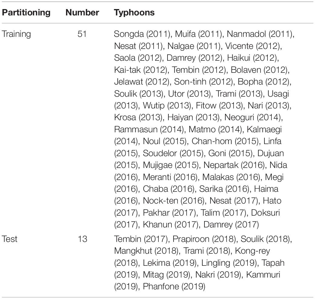
Table 1. Partitioning of typhoons into training and validation sets.

Methodology

Convolutional Long Short-Term Memory Network

The LSTM is a special type of recurrent neural network (RNN). The basic idea of the LSTM is to control the input and output of information in the cell by introducing three gates: input, output, and forget gates. These are used to control the flow of information between the cells. Respectively, the input gate determines the value to be updated, the output gate mainly controls the information transmission to the next cell, and the forget gate selectively forgets the information in the information transfer. The LSTM has two states, cell state (c_t) and hidden state (h_t), which are related to c_t–1 and h_t–1 of the previous cell (Hochreiter and Schmidhuber, 1997). These structural features enable the LSTM to learn long-term temporal information and avoid long-term dependence problems. Since there are many ways to propagate gradients in the LSTM, vanishing and exploding gradient problems can be better avoided. The following are the information state transfer formulae in one cell of the LSTM:

$$i_t=\mathrm{\sigma }(W_{xi}{x}_t+W_{hi}{h}_{t-1}+W_{ci}\circ c_{t-1}+b_i)(1)$$

$$f_t=\mathrm{\sigma }(W_{xf}{x}_t+W_{hf}{h}_{t-1}+W_{cf}\circ c_{t-1}+b_f)(2)$$

$$c_t=f_t\circ c_{t-1}+i_t\circ tanh(W_{xc}{x}_t+W_{hc}{h}_{t-1}+b_c)(3)$$

$$o_t=\mathrm{\sigma }(W_{xo}{x}_t+W_{ho}{h}_{t-1}+W_{co}\circ c_t+b_o)(4)$$

$$h_t=o_t\circ tanh(c_t)(5)$$

where i_t represents the input gate, f_t represents the forget gate, o_t represents the output gate, c_t represents the state of the current moment, c_t–1 represents the state of the previous moment, h_t represents the final output, W represents the weight coefficient for a given gate, b represents the corresponding bias coefficient for a given gate, ∘is the Hadamard product, and σ is the sigmoid function.

Presently, the LSTM is widely used in time series forecasting. However, when the LSTM is applied to 2D data, if it is expanded into full connected layer processing, it not only consumes substantial computing resources but also it is difficult to capture the spatial correlation and spatial characteristics of the 2D space field (Shi et al., 2015). To overcome these deficiencies, Shi et al. (2015) replaced the FC-LSTM layers with a convolutional structure, leading to the development of the ConvLSTM network. The primary difference between the LSTM and the ConvLSTM is the replacement of matrix multiplication by a convolutional operation:

$$i_t=\mathrm{\sigma }(W_{xi}*X_t+W_{hi}*h_{t-1}+W_{ci}\circ c_{t-1}+b_i)(6)$$

$$f_t=\mathrm{\sigma }(W_{xf}*X_t+W_{hj}*h_{t-1}+W_{cf}\circ c_{t-1}+b_f)(7)$$

$$c_t=f_t\circ c_{t-1}+i_t\circ tanh(W_{xc}*X_t+W_{hc}*h_{t-1}+b_c)(8)$$

$$o_t=\mathrm{\sigma }(W_{xo}*X_t+W_{ho}*h_{t-1}+W_{co}\circ c_t+b_o)(9)$$

$$h_t=o_t\circ tanh(c_t)(10)$$

where * is convolution operator.

Convolution operation can extract the spatial characteristics of the data, while the LSTM can extract the temporal variability of the data. Therefore, the ConvLSTM has the ability to well depict both a variable’s spatiotemporal characteristics and is hence highly suitable for regional ocean wave predictions.

Architecture of the ConvLSTM Model for Wave Forecasts

In this paper, a regional wave prediction model is established based on the ConvLSTM network (Figure 1). The SWH data of three continuous time steps are taken as the input data. The SWH data at a certain time in the future are output through three ConvLSTM layers and finally through a convolution layer for a total of four layers. For example, SWH at times 13:00, 14:00, and 15:00 on January 1, 2018 is given (input) to the model and SWH at time 16:00 is predicted (output). To improve the model’s ability to capture non-linearities, the recursive linear unit (ReLU) is employed as the activation function in each layer, with the hard sigmoid used as the activation function in the loop step. The convolutional kernels of each of four layers are set to 5 * 5, 3 * 3, 3 * 3, and 5 * 5, respectively, to capture different characteristics at different spatial scales. The root-mean-square error (RMSE) is used as the loss function during model training, the number of epochs is set to 100, and all other remaining parameters remain constant throughout all training exercises.

FIGURE 1

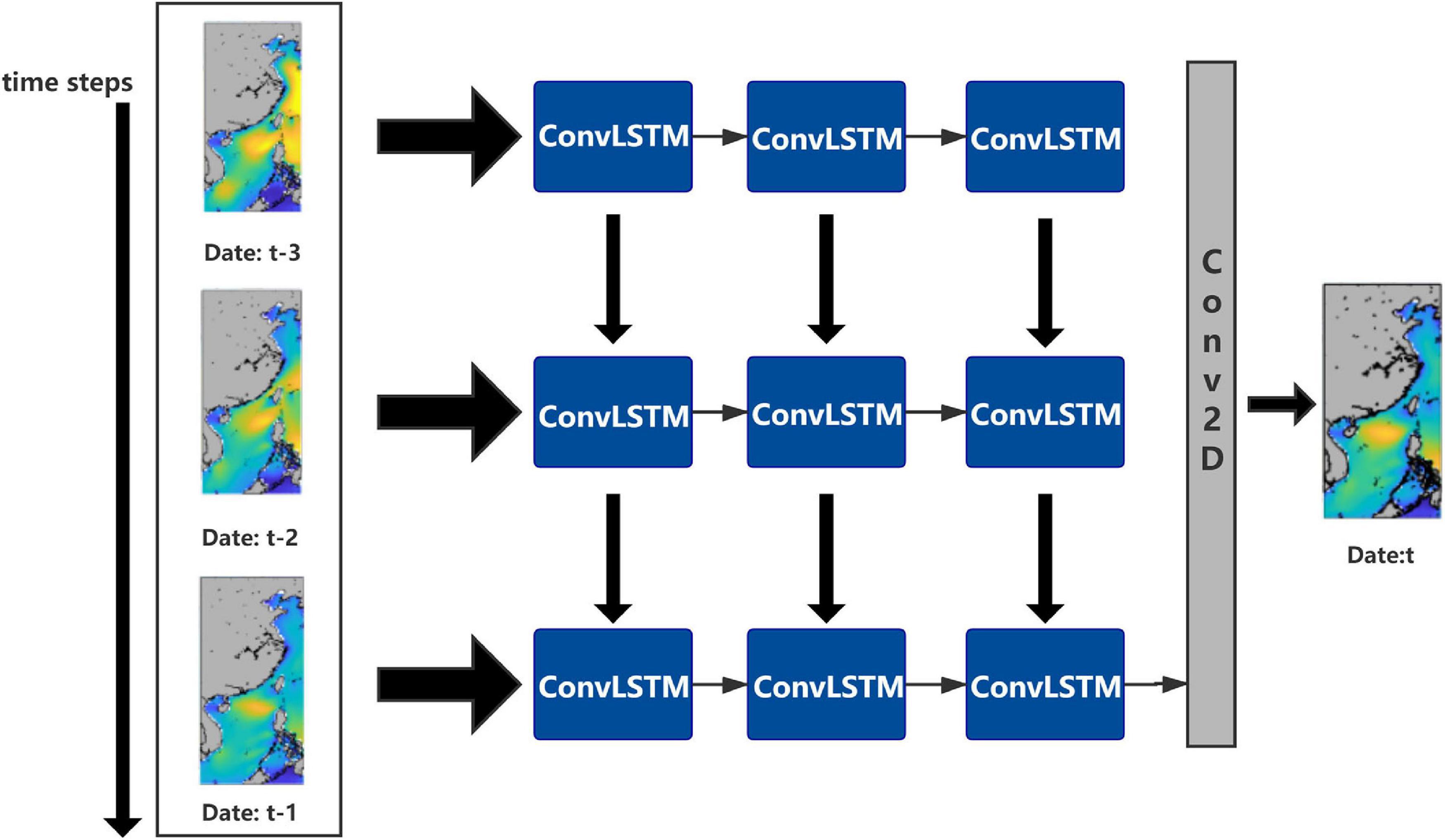
Figure 1. Schematic of the SWH prediction model based on the ConvLSTM.

Data Pre-processing

To improve the training dataset quality, the WW3 SWH reanalysis product is linearly interpolated from a resolution of 1/2°* 1/2° to 1/4°* 1/4°. The input data are wave field data of three consecutive time steps. According to the different prediction time steps (e.g., 1, 2, and 3 h), the corresponding training dataset and verification set are generated using the data from 2011 to 2018, in which the data volume ratio of training set and verification set is 4:1. For predictions of SWH, the data for the year of 2019 are the test set, which are excluded from the model training to ensure relative independence between the training and test datasets.

Evaluation Functions

In order to better evaluate the accuracy of model forecasts, this article defines the following evaluation functions. Difference error (DR), mean absolute error (MAE), RMSE, spatially averaged RMSE (SARMSE), and spatially averaged mean absolute percentage error (SAMAPE) are used to evaluate the deviation between predicted values and WW3 reanalysis data. In addition, the spatially averaged correlation coefficient (SACC) is used to measure the linear correlation between the predicted values and WW3 values. The expressions of the above variables are as follows:

$$DR(i,j)=h_p(i,j)-h_m(i,j)(11)$$

$$MAE=\frac{1}{I\cdot J}\sum _{i=1}^I\sum _{j=1}^J\left|h_p(i,j)-h_m(i,j)\right|(12)$$

$$RMSE=\sqrt{\frac{1}{I\cdot J}\sum _{i=1}^I\sum _{j=1}^J{(h_p(i,j)-h_m(i,j))}^2}(13)$$

$$SARMSE=\frac{1}{K}\sum _{k=1}^K\sqrt{\frac{1}{I\cdot J}\sum _{i=1}^I\sum _{j=1}^J{(h_p(i,j,k)-h_m(i,j,k))}^2}(14)$$

$$SAMAPE=\frac{1}{n}\sum _{k=1}^n\frac{1}{I\cdot J}\sum _{i=1}^I\sum _{j=1}^J\frac{\left|h_p(i,j,k)-h_m(i,j,k)\right|}{h_m(i,j,k)}\times 100\%(15)$$

$$SACC=$$

$$\frac{\frac{1}{n}{\sum }_{k=1}^n(h_p(i,j,k)-\overline{h_p(i,j,k)})(h_m(i,j,k)-\overline{h_m(i,j,k)})}{\begin{array}{c}\hfill \sqrt{\frac{1}{n}{\sum }_{k=1}^n{(h_p(i,j,k)-\overline{h_p(i,j,k)})}^2}\hfill \\ \hfill \sqrt{\frac{1}{n}{\sum }_{k=1}^n{(h_m(i,j,k)-\overline{h_m(i,j,k)})}^2}\hfill \end{array}}(16)$$

where i and j denote the coordinates of space lattice points, k denotes cases, n represents the total number of cases, I denotes the total number of latitudinal lattice points, and J denotes the total number of meridional lattice points. DR(i,j) is the error value of a certain point in space, h_p(i,j) is the SWH value predicted based on the ConvLSTM model, and h_m(i,j) is the WW3 SWH value corresponding to a certain point in space. h_p(i,j,k) represents the ConvLSTM model-predicted SWH at a certain point in the case space, $\overline{h_p(\text{i},\text{j},\text{k})}$ represents the mean SWH predicted by the ConvLSTM model at a certain point in the case space, and h_m(i, j, k) represents the SWH of WW3 at a certain point in the case space. $\overline{h_m(\text{i},\text{j},\text{k})}$ represents the mean SWH of WW3.

Results

In this study, the ConvLSTM is applied to wave forecasting in the northwestern Pacific Ocean under both normal and extreme conditions. This section is divided into two subsections. In Section “Wave Forecast Under Normal Conditions,” the test set results are presented and discussed for the normal condition. In Section “Wave Forecast Under Extreme Conditions,” the wave forecast is presented for extreme condition (i.e., typhoon cases).

Wave Forecast Under Normal Conditions

First, we discuss the performance of the ConvLSTM algorithm in predicting SWH under normal conditions. Figures 2, 3 show examples of the ConvLSTM wave forecasts, which all use SWH data at 5:00, 6:00, and 7:00 (UTC) on October 3, 2019, as inputs. Figures 2A,D,G correspond to the spatial distribution of the forecasted SWH after 1, 3, and 6 h. Figures 2B,E,H show the spatial distribution of the WW3 data that corresponds to the forecast moments. The errors between the forecast and the WW3 data are displayed in Figures 2C,F,I. In the 1-h forecast (Figures 2A,B), the model results show good consistency with the baseline in terms of both the magnitude of the wave height and the spatial distribution. In general, the 1-h forecast error fluctuates within −0.1 to 0.1 m (Figure 2C). Relatively high values are observed in the open sea and Bohai Sea. Low SWH covers the rest of the domain. A slightly larger error can be seen only in the Yellow Sea. We can identify that when forecast time span is increased to 3 h, a high degree of accuracy is obtainable in the Yellow and East China Seas (Figures 2D,E). The large deviations of the forecasts from the WW3 correspond to the high SWH area in the Bohai Sea (Figures 2G,H), with a large forecast error also noted in Figure 2I. The 6-h wave forecasts underestimate the SWH noticeably in the Bohai and South China Seas, while the forecasts overestimate the SWH in the Yellow and the East China Seas. Figure 3 shows the predicted and the WW3 SWH at each sample point in space at the three moments from Figure 2 from low to high latitudes. It can be found that the predicted spatial distribution of SWH at these three moments is basically consistent with that from the WW3. From Figure 3A, the 1-h forecast has the best performance, a good consistency is observed between forecast and the WW3 data with MAE, RMSE, and the correlation at 0.03 m, 0.04 m, and 0.997, respectively. The forecast values are smaller than the WW3 baseline. A similar pattern can also be seen in Figure 3B. This deviation causes the larger MAE and RMSE of the 3-h forecast compared with the 1-h forecast, and the correlation decreases to 0.991. At the 6-h window, the least accurate forecast was observed that had a correlation coefficient of 0.962.

FIGURE 2

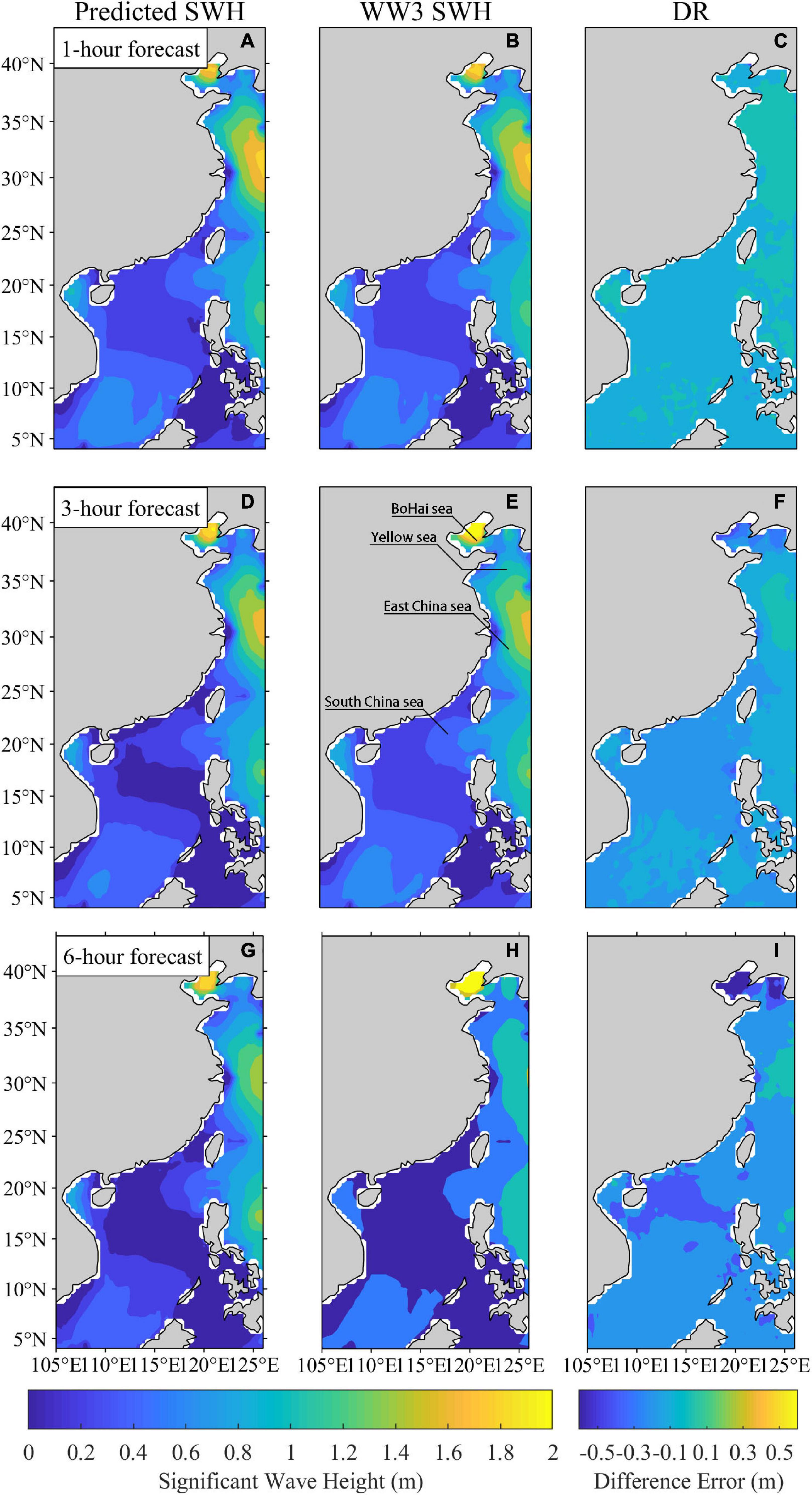
Figure 2. Comparison of SWH from the WW3 and the ConvLSTM algorithm prediction. (A,D,G) are 1-, 3-, and 6-h predictions, respectively, based on the SWH data at 5:00, 6:00, and 7:00 on October 3, 2019. (B,E,H) The WW3 wave fields at the corresponding forecast moments. (C,F,I) are the difference error between the WW3 data and the predictions.

FIGURE 3

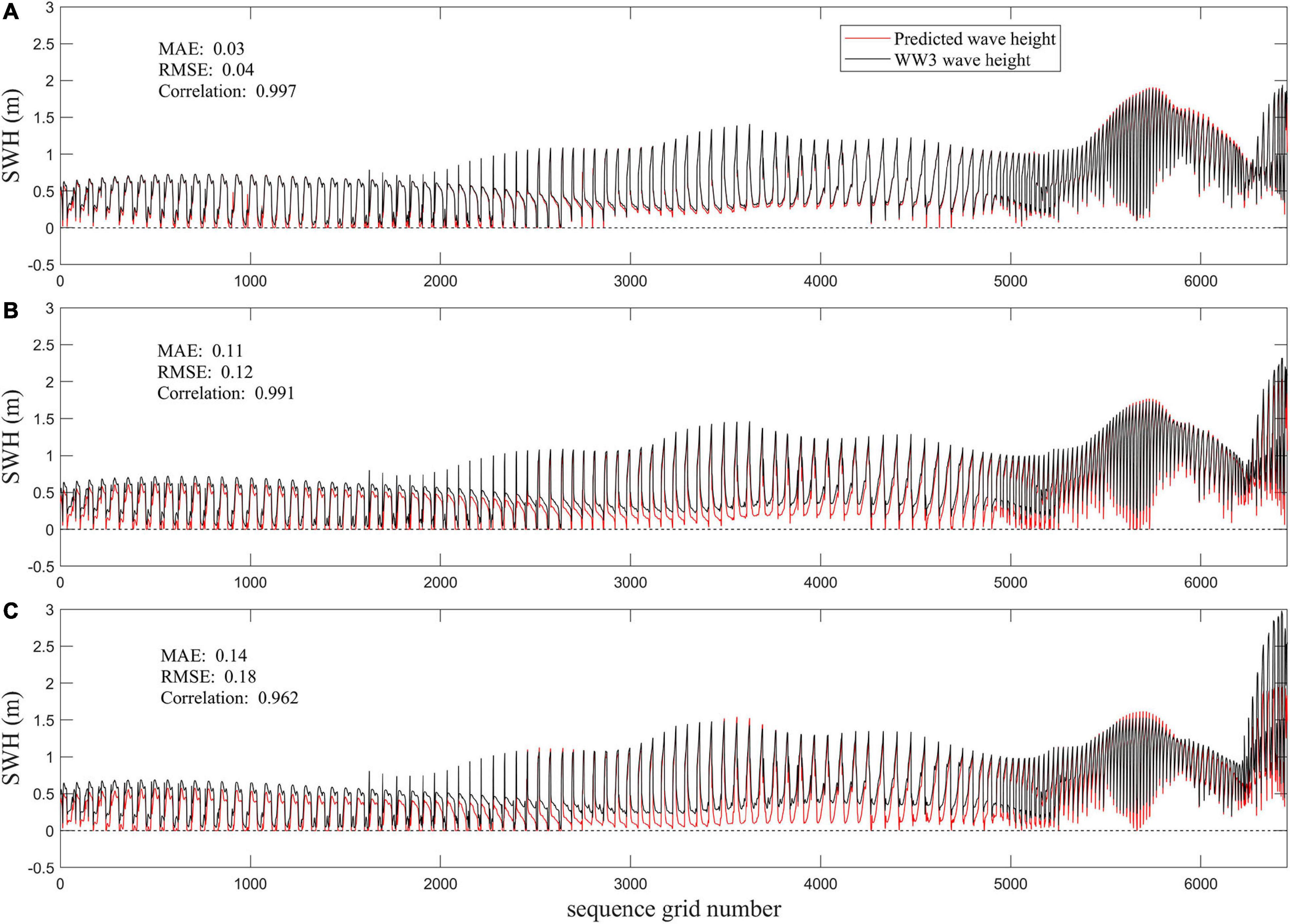
Figure 3. Predicted (red line) vs. the WW3 (black line) SWH throughout the study area for (A) 1-, (B) 3-, and (C) 6-h forecast moments.

To further illustrate this model’s performance, it is necessary to discuss the impact of the forecast time span on forecast errors. The forecast time span is the time scale of wave forecasting. Figure 4 shows the error variations with the forecast time span in 2019, which is based on the training and validation sets for the period from 2011 to 2014. It can be seen that the SARMSE increases as the forecast time span increases, while this trend is reversed for SACC. The SARMSE for the forecast time span of less than 6 h is less than 0.2 m, with the SACC close to 1.0, the forecast accuracy is still high, so in this case the spatial characteristics of the wave field from the training set at the three moments can better respond to the changing wave field trends of the next 6 h that ensure a relatively high forecast accuracy. When the forecast time span increases to 12 h, the SARMSE gradually increases to 0.29 m. However, when the forecast time span exceeds 12 h and increases to 24 h, the model still keeps the SACC around 0.8, but the SARMSE is close to 0.6 m. The adaptability of the training samples to forecast larger time spans decreases, which may be due to a great number of unknown factors encumbering the training set from accurately and adequately responding to a rapidly evolving wave field. The above results indicate that the model still requires further experiments, testing and evaluation to improve forecast beyond 12 h. The selection of training samples can be adjusted to improve the model performance, which will be discussed in Section “Discussion.” Therefore, it can be concluded that the larger the forecast time span, the larger SARMSE and the smaller SACC.

FIGURE 4

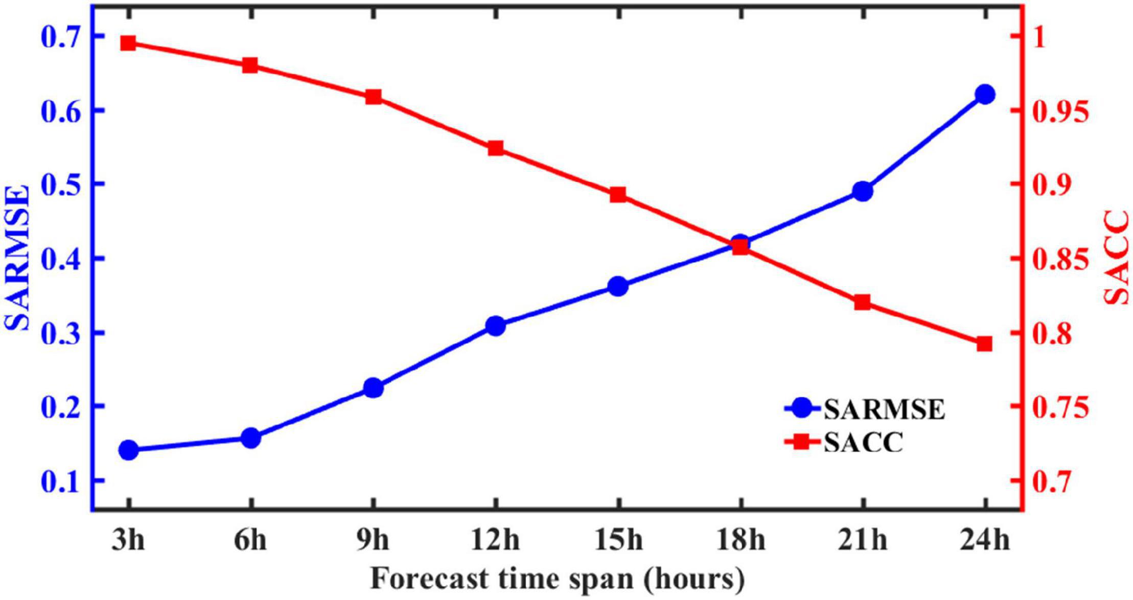
Figure 4. Variations in the SARMSE (blue) and SACC (red) of each training result with forecast time span.

In the preceding paragraph, the SARMSE is presented for the discussion of the model performance. To better represent the model errors, the changes of SAMAPE with the forecast time span are listed in Table 2, which shows that the changes of SAMAPE are similar to those of the SARMSE. The SAMAPE increases and the forecast accuracy decreases as the forecast time span increases (Table 2). When the forecast time span is 3 h, the SAMAPE is only 11.1%, and when the forecast time span increases to 24 h, the SAMAPE is 62.8%.

TABLE 2

Table 2. Changes of SAMAPE with forecast time span.

Wave Forecast Under Extreme Conditions

Typhoons, generated over tropical and subtropical oceans, produce intense surface wind speed that can force wind waves to grow to approximately 10 m in height. Along the coast of China, typhoons mainly affect the South China Sea in May, June, and October to December, and usually affect southeastern coastlines and even the coastal areas in the East China Sea from July to September (Lu and Qian, 2012). Due to the large discrepancy between normal and extreme (typhoon-induced) wave states, in conjunction with the low frequency of typhoons in proportion to the full dataset, the ConvLSTM trained by the data under the normal conditions may fail to learn all typhoon characteristics and so typhoon-induced SWH forecasts may be flawed. In this section, we propose that the ConvLSTM can be trained by the typhoon-induced wave data for the wave forecast under the extreme conditions.

To verify this hypothesis, we have defined Model 1 and Model 2, where Model 1 is trained by the normal-condition wave data and Model 2 is trained by typhoon-induced waves. For the experiments, their forecast time spans are held at a 3-h constant. Figure 5 shows the forecast effect of using Model 1 and Model 2 using snapshots of Typhoons Lekima that occurred in the East China Sea at 18:00 on August 8, 2019 and Tembin that occurred in the South China Sea at 21:00 on December 24, 2017. Comparing Figures 5A,D, with Figures 5B,E, we can find that although Model 1 is able to capture the primary features of the wave field near the typhoon center, the forecast results at the center are generally smaller than the WW3, large SWH generated near the center is not adequately reproduced. Far from the typhoon center where the system has a reduced impact on the waves, Model 1 can more adequately capture SWH patterns than at the typhoon center. By contrast, Model 2 is better able to capture the spatial patterns of SWH during typhoons as observed from Figures 5B,E. This, however, comes at a minor cost of slightly overestimating SWH at the typhoon center. That is, the area around the highest values in Figures 5B,E are slightly larger than that in Figures 5C,F. There are insufficient examples of typhoon-induced SWH in the Model 1 dataset due to the low frequency and short duration of typhoons and thus in all training datasets, there were insufficient examples of typhoon-induced SWH for Model 1 to learn from. Consequently, typhoon characteristics are difficult to be extracted from Model 1. Generally, both in the center of the typhoon and surrounding areas, wave forecasts were greatly improved in Model 2 as compared to Model 1.

FIGURE 5

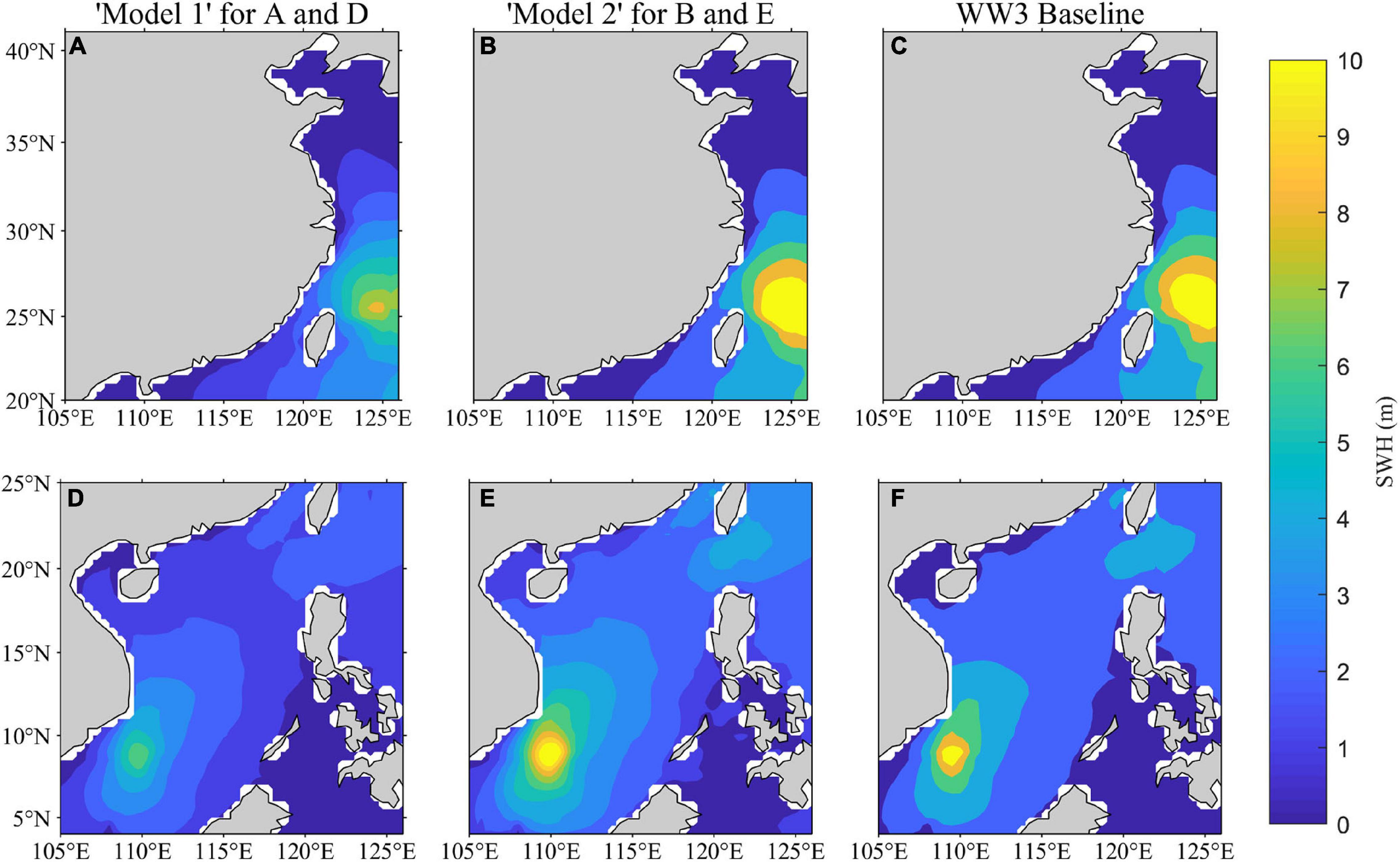
Figure 5. The SWH prediction results of Model 1 and Model 2 under typhoon conditions in the East China Sea and South China Sea. (A–C) SWH of Typhoon “Lekima” over the East China Sea at 18:00 on August 8, 2019. (D–F) SWH of Typhoon “Tembin” over the South China Sea at 21:00 on December 24, 2017.

To further illustrate the difference in the wave forecasts with Model 1 and Model 2 under extreme state, changes of the forecast time span of Model 1 and Model 2 are examined. The error statistic results (SACC, SARMSE, and SAMAPE) are shown in Figures 6A–C, respectively. In Figure 6A, SACC of both Model 1 and Model 2 decreases almost linearly with the increase of the forecast time span, but the SACC of Model 2 is always higher than that of Model 1. In Figures 6B,C, both SARMSE and SAMAPE of Model 1 and Model 2 show an almost linear increasing trend. The SARMSE of Model 2 within 6 h is less than 0.5 m and the SAMAPE is less than 20%, while the SARMSE from Model 1 is at about 1 m and the SAMAPE at approximately 40%. When the forecast time span is 24 h, the SAMAPE of Model 2 becomes slightly higher than that of Model 1.

FIGURE 6

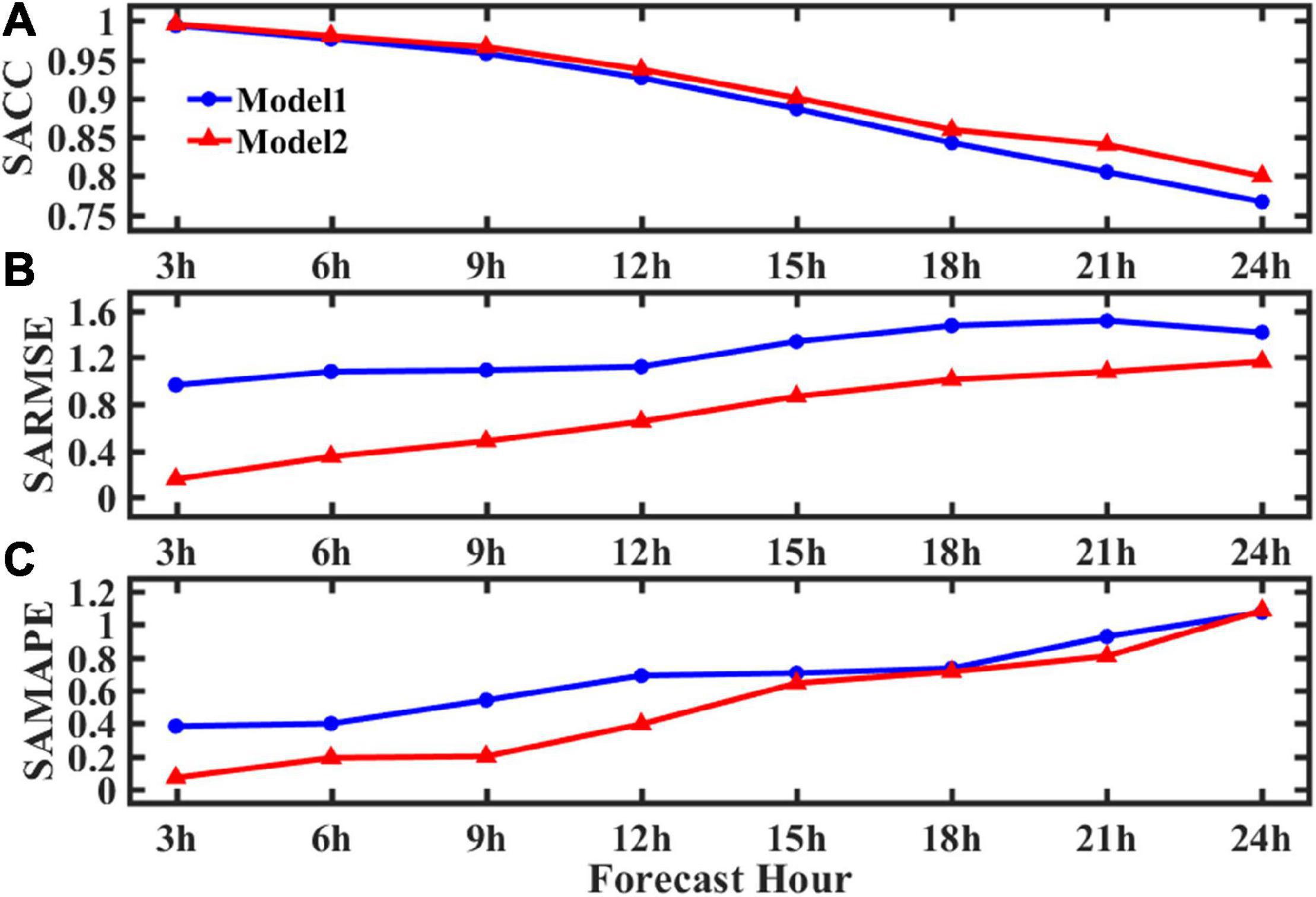
Figure 6. Error statistics of Models 1 and 2 relative to the WW3 baseline. (A) SACC, (B) SARMSE, and (C) SAMAPE.

In summary, for within the 24-h forecast under typhoon conditions, Model 2 shows better forecast capability than that of Model 1. Compared with Model 1, the prediction error of Model 2 is smaller and the prediction in the typhoon-affected area is more accurate. This is because the training set of Model 1 is mainly from the wave data under normal conditions including few typhoon-induced wave data. As a result, Model 1 cannot accurately capture wave characteristics under typhoon conditions.

Discussion

In this paper, an intelligent forecast model for waves in the South China Sea and East China Sea based on the ConvLSTM algorithm is established. The model relies on wave hindcasts as input to forecast wave spatial distributions. It can be seen from the results in Section “Results” that the prediction of the SWH based on the ConvLSTM is feasible under normal and extreme conditions. The 1–12-h results are acceptable, with relatively larger errors in 24-h forecasts.

Figure 7 discusses the model’s performance from the input data time span and the training sets time span, respectively. We first discuss the input data time span that represents the input data quantity. For example, “2 h” (Figure 7A) means the continuous input of 2-h wave field data for forecasting. Figure 7A shows the forecast error results against the input data time span. When the input data time span is 2 h, the SACC is low (about 0.97), and the SARMSE is large (about 0.22). Since the data volume of 2-h wave field data is small, the model reproduces few wave features during the training process, which leads to low forecast accuracy. As the input data time span increases, the SACC improves, and the SARMSE gradually decreases, stabilizes, but increases at 5-h mark. The reason is that if the amount of input data is too much, it causes data redundancy, which cannot further improve forecast accuracy. Therefore, it can be seen that 3 h is the optimal selection for the input data time span in terms of the forecast accuracy and computing time cost. This selection of the input data time span guarantees the forecast accuracy, in addition to saving computational resources and minimizing the amount of time required for computations to ensure the forecast timeliness.

FIGURE 7

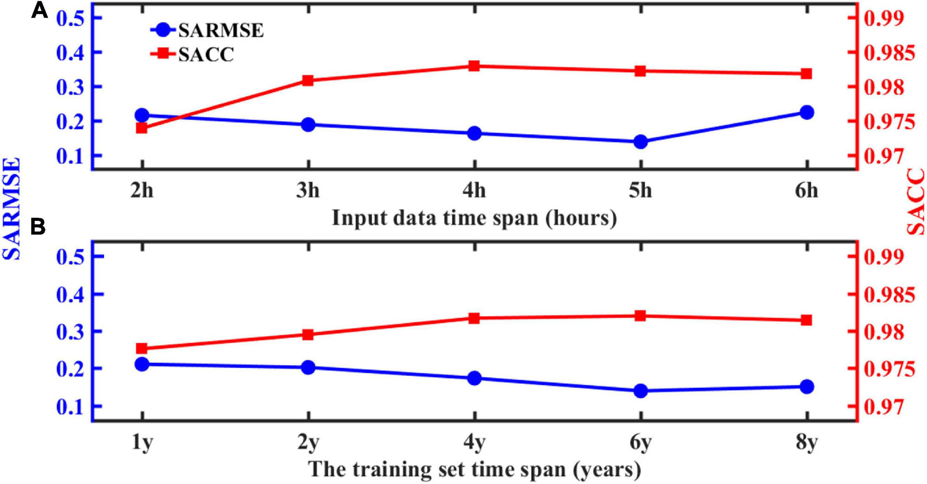
Figure 7. (A) Changes in SARMSE and SACC with the time span of the input data. (B) Changes in SARMSE and SACC with the time span of the training set data.

Because of the difference in the characteristics of the different training set time span, it is necessary to find the optimal training set time span. We set the forecast time span to 6 h and then select the same number of data samples under different time spans as training sets. Figure 7B shows the error results under different training set time spans. Generally, with the increase in the training set time span, the SARMSE has a downward trend, and the SACC has an upward trend. When the training set time span is 1y, the SARMSE is 0.21 m, and the SACC is about 0.97. As the training set time span increases, the SARMSE gradually decreases and stabilizes at about 0.15 m. When the training set time span exceeds 4 years, the model performance has not greatly been improved. So, this study chooses 4 years as the training set time span. Therefore, combining the input data and the training set time span, the SWH prediction based on the ConvLSTM does not require a very large training set, nor does it require long-term data as input. So, this method not only improves the forecast efficiency but also greatly saves computational resources. This model is trained on the GeForce RTX 2080 Ti, the training of a single model takes about 2 h, and it only takes less than 20 s to complete the prediction of the test set in 2019. Therefore, the SWH prediction based on the ConvLSTM is feasible and efficient.

The present study only uses SWH data to predict the SWH; however, the generation of waves is closely related to the overlying wind field, and SWH can also be predicted by wind and other variables (Wang et al., 2021), but this relationship is specific to wind waves as may be caused by typhoons. Swell contamination of the wave field can weaken the wind–wave relationship (Niu and Feng, 2021) and thus it is necessary to introduce other input variables. Consequently, in future research, additional physical phenomena such as ocean currents can be added to improve wave forecasts. Additionally, due to the coarse nature of the input data, no wave information on any coastline was available and thus restricts its operational usage for coastal communities. The usage of a high-resolution wave model can be used in place of the reanalysis dataset that can provide coastal wave information and should be pursued in future research.

Data Availability Statement

The datasets presented in this study can be found in online repositories. The names of the repository/repositories and accession number(s) can be found below: https://coastwatch.pfeg.noaa.gov/erddap/griddap/NWW3_Global_Best.html.

Author Contributions

SZ and WX designed the experiment. SZ, YL, YW, YZ, and NH contributed to the data analysis and the writing of the first draft of the manuscript. CD is the creator and person in charge of the project, directing experimental design, data analysis, thesis writing, and revision. All authors read and agreed to the final text.

Funding

This study was supported by the project supported by the Southern Marine Science and Engineering Guangdong Laboratory (Zhuhai) (SML2020SP007), the Key Program of Marine Economy Development (Six Marine Industries) Special Foundation of Department of Natural Resources of Guangdong Province [GDNRC(2020)049], the National College Students’ Platform for Innovation and Entrepreneurship Training Program (202010300017Z), the Jiangsu Province College Students’ Platform for Innovation and Entrepreneurship Training Program (202010300017Z), and the NUIST Students’ Platform for Innovation and Entrepreneurship Training Program (202010300017Z).

Conflict of Interest

The authors declare that the research was conducted in the absence of any commercial or financial relationships that could be construed as a potential conflict of interest.

Acknowledgments

The SWH data were collected from NOAA, and the relevant typhoon data were obtained from the Central Meteorological Observatory.

Footnotes

1. ^ https://coastwatch.pfeg.noaa.gov/erddap/griddap/NWW3_Global_Best.html
2. ^ http://typhoon.nmc.cn/web.html

References

Aparna, S. G., D’Souza, S., and Arjun, N. B. (2018). Prediction of daily sea surface temperature using artificial neural networks. Int. J. Remote Sens. 39, 4214–4231. doi: 10.1080/01431161.2018.1454623

CrossRef Full Text | Google Scholar

Choi, H., Park, M., Son, G., Jeong, J., Park, J., Mo, K., et al. (2020). Real-time significant wave height estimation from raw ocean images based on 2D and 3D deep neural networks. Ocean Eng. 201:107129. doi: 10.1016/j.oceaneng.2020.107129

CrossRef Full Text | Google Scholar

Emmanouila, S., Aguilarc, S. G., Nane, G. F., and Schoutenc, J. J. (2020). Statistical models for improving significant wave height predictions in offshore operations. Ocean Eng. 206:107249. doi: 10.1016/j.oceaneng.2020.107249

CrossRef Full Text | Google Scholar

Fan, S., Xiao, N., and Dong, S. (2020). A novel model to predict significant wave height based on long short-term memory network. Ocean Eng. 205:107298. doi: 10.1016/j.oceaneng.2020.107298

CrossRef Full Text | Google Scholar

Ham, Y. G., Kim, J. H., and Luo, J. (2019). Deep learning for multi-year ENSO forecasts. Nature 573, 568–572. doi: 10.1038/s41586-019-1559-7

PubMed Abstract | CrossRef Full Text | Google Scholar

Hochreiter, S., and Schmidhuber, J. (1997). Long short-term memory. Neural. Comput. 9, 1735–1780. doi: 10.1162/neco.1997.9.8.1735

PubMed Abstract | CrossRef Full Text | Google Scholar

Kaloop, M. R., Kumar, D., Zarzoura, F., Roy, B., and Hu, J. W. (2020). A wavelet–particle swarm optimization–extreme learning machine hybrid modeling for significant wave height prediction. Ocean Eng. 213:107777. doi: 10.1016/j.oceaneng.2020.107777

CrossRef Full Text | Google Scholar

Kim, J., Kim, K., Cho, J., Kang, Y. Q., Yoon, H. J., and Lee, Y. W. (2018). Satellite-based prediction of arctic sea ice concentration using a deep neural network with multi-model ensemble. Remote Sens. 11:19. doi: 10.3390/rs11010019

CrossRef Full Text | Google Scholar

Kim, Y. J., Kim, H. C., Han, D., Lee, S., and Im, J. (2020). Prediction of monthly Arctic sea ice concentrations using satellite and reanalysis data based on convolutional neural networks. Cryosphere 14, 1083–1104. doi: 10.5194/tc-14-1083-2020

CrossRef Full Text | Google Scholar

Lee, S. W., and Kim, H. Y. (2020). Stock market forecasting with super-high dimensional time-series data using ConvLSTM, trend sampling, and specialized data augmentation. Expert. Syst. Appl. 161:113704. doi: 10.1016/j.eswa.2020.113704

CrossRef Full Text | Google Scholar

Londhe, S. N., and Panchang, V. J. (2006). One-day wave forecasts based on artificial neural networks. J. Atmos. Ocean. Technol. 23, 1593–1603. doi: 10.1175/JTECH1932.1

CrossRef Full Text | Google Scholar

Lu, B., and Qian, W. H. (2012). Seasonal lock of rapidly intensifying typhoons over the South China offshore in early fall. Chin. J. Geophys. 55, 1523–1531. doi: 10.6038/j.issn.0001-5733.2012.05.009

CrossRef Full Text | Google Scholar

Lu, P., Liang, S., Zou, G., Zheng, Z., and Zou, P. (2019). M-LSTM, a hybrid prediction model for wave heights. J. Nonlinear. Convex. A 20, 775–786.

Google Scholar

Majd, M., and Safabakhsh, R. (2019). Correlational convolutional LSTM for human action recognition. Neurocomputing 396, 224–229. doi: 10.1016/j.neucom.2018.10.095

CrossRef Full Text | Google Scholar

Mondon, E., and Warner, P. (2009). Synthesis of a validated nearshore operational wave database using the archived NOAA Wave watch III ocean model data and swan nearshore model. J. Coastal Res. 2009, 1015–1019. doi: 10.2307/25737940

CrossRef Full Text | Google Scholar

Niu, Q., and Feng, Y. (2021). Relationships between the typhoon-induced wind and wave in the northern South China Sea. Geophys. Res. Lett. 48:e2020GL091665. doi: 10.1029/2020GL091665

CrossRef Full Text | Google Scholar

Peng, Y., Tao, H., Li, W., Yuan, H., and Li, T. (2020). dynamic gesture recognition based on feature fusion network and variant convLSTM. IET Image. Process. 14, 2480–2486. doi: 10.1049/iet-ipr.2019.1248

CrossRef Full Text | Google Scholar

Shi, X., Chen, Z., Wang, H., Yeung, D. Y., Wong, W. K., and Woo, W. C. (2015). “Convolutional lstm network: a machine learning approach for precipitation nowcasting,” In Proceedings of the 29th Annual Conference in Neural Information Processing sSystems, Montreal, MTL, 802–810.

Google Scholar

Triasdian, B., Indartono, Y. S., Ningsih, N. S., and Novitasari, D. (2019). Device selection of the potential wave energy site in indonesian seas. IOP Conf. Ser. Earth Environ. Sci. 291:012040. doi: 10.1088/1755-1315/291/1/012040

CrossRef Full Text | Google Scholar

Wang, H., Yang, J., Zhu, J., Ren, L., Liu, Y., Li, W., et al. (2021). Estimation of significant wave heights from ASCAT scatterometer data via deep learning network. Remote Sens. 135:195. doi: 10.3390/rs13020195

CrossRef Full Text | Google Scholar

Xu, G., Cheng, C., Yang, W., Xie, W., Kong, L., Hang, R., et al. (2019). Oceanic eddy identification using an AI scheme. Remote Sens. 11:1349. doi: 10.3390/rs11111349

CrossRef Full Text | Google Scholar

Zeng, X., Li, Y., and He, R. (2015). Predictability of the loop current variation and Eddy shedding process in the Gulf of Mexico using an artificial neural network approach. J. Atmos. Ocean. Technol. 32, 1098–1111. doi: 10.1175/JTECH-D-14-00176.1

CrossRef Full Text | Google Scholar

Zheng, C., and Li, C. (2015). Variation of the wave energy and significant wave height in the China Sea and adjacent waters. Renew. Sust. Energ. Rev. 43, 381–387. doi: 10.1016/j.rser.2014.11.001

CrossRef Full Text | Google Scholar

Zheng, G., Li, X., Zhang, R., and Liu, B. (2020). Purely satellite data-driven deep learning forecast of complicated tropical instability waves. Sci. Adv. 6:1482. doi: 10.1126/sciadv.aba1482

PubMed Abstract | CrossRef Full Text | Google Scholar