Regional Reef Fish Survey Design and Scaling Using High-Resolution Mapping and Analysis

Introduction

Coral reefs are undergoing continual and rapid changes caused by coastal development, resource use, and climate change (Knowlton, 2001). Both the benthic habitat and occupants of that habitat need ecologically robust monitoring in order to assess patterns and rates of change for management and conservation decision-making (Brownscombe et al., 2019). However, the approaches available for most monitoring programs are limited by issues of access, cost, and repeatability. Reef habitat and fish monitoring is usually carried out by divers using visual and/or photographic data collection techniques (e.g., Flower et al., 2017; Friedlander et al., 2018; Gorospe et al., 2018). These methods often yield data on specific locations at discrete points in time, but they are difficult to scale up to derive ecosystem-level patterns and trends over time (Edgar et al., 2016).

Habitat complexity of coral reefs is driven by spatial and temporal variability in available substrate, such as rocks, sand, hard calcareous surfaces, live coral and algal cover, and environmental variables such as depth, rugosity, water quality, and light availability (Kovalenko et al., 2012). These drivers interact and create feedbacks on populations of fish, invertebrates, and other organisms that inhabit the reef. Quantitative monitoring of these drivers and their interactions remains a major challenge due to the sheer extent, variability and complexity of coral reef ecosystems. Recent advances in airborne imaging spectroscopy (hyperspectral) mapping of reefs, whereby the ocean surface is imaged in hundreds of narrow, contiguous spectral bands, have yielded spatially explicit information on the location and extent of key determinants of reef habitat including live coral and macroalgal cover, sand cover, water depth, and a range of 3D habitat complexity metrics to more than 16 m (52 ft) depth (Asner et al., 2020a,b, 2021). In combination with previously mapped coastal land features, these benthic mapping capabilities provide an improved means to monitor changes in habitat over time at large ecological scales. While the approach is limited to very few airborne systems today, the same technology is in development for space-based deployment (Thompson et al., 2020), which will provide opportunities to greatly improve reef habitat mapping worldwide, and highlight a need to develop applications of this technology as soon as possible.

Combinations of multiple reef and terrestrial habitat maps provide an opportunity to develop, test and improve fisheries monitoring in spatially explicit ways. Specifically, high-resolution mapping allows for stratified-random sampling of reef species (fish, invertebrates, and others), which involves dividing the entire ecosystem into smaller subgroups known as strata. These strata represent habitats that differ significantly from one another, and need to be sampled separately. While this sampling approach is commonly applied in terrestrial ecosystems (e.g., Shiver and Borders, 1996; Tomppo et al., 2008), aquatic applications have successfully utilized similar approaches with multispectral remote sensing data (Friedlander et al., 2007; Purkis et al., 2008). Map-based approaches provide an avenue for regional downscaling to derive randomly located sites for monitoring that accurately represent habitat variability across the entire ecosystem (e.g., Mellin et al., 2009; Knudby et al., 2011). Map-based approaches also allow upscaling of field-based observations to generate regional estimates that integrate habitat complexity over space and time, which is central to marine spatial planning, fisheries management, reef restoration and numerous other activities.

Here we build off a past approach using a large-scale ecosystem mapping and sampling scheme, driven by airborne hyperspectral remote sensing data (Asner et al., 2017), to scale surveys of reef fish over an extensive, ecologically complex reef ecosystem in the Hawaiian Islands. The method provides detailed maps of the most important habitat-generating organisms in an ecosystem (e.g., trees in forests, corals on reefs), and utilizes these maps along with other geospatial information to sample and then upscale field-based surveys of habitat occupants (e.g., birds in forests, fish on reefs) to the regional level. Accurate regional stock assessments of reef fishes are critical for effective management and conservation of coral reefs (Bacheler et al., 2017). Using new aircraft-based hyperspectral remote sensing and other environmental maps, combined and analyzed into reef classes or strata, we carried out a field sampling campaign to assess reef fish diversity and biomass, two important metrics of fishery composition and condition. We then upscaled the field data using the mapped strata to estimate total fish diversity and biomass as well as spatial variation in both sets of ecological metrics. Finally, we reduced the number of field sites incrementally to assess the minimum level of monitoring required to maintain statistically robust estimates of fish diversity and biomass. Our findings uniquely generate specific recommendations for future monitoring of Hawaiian coral reef ecosystems over time, and the approach provides a methodology that can be applied in any coral reef ecosystem.

Materials and Methods

Study Region

The District of South Kona is located in the southwestern portion of Hawai‘i Island in the eight Main Hawaiian Islands (Figure 1). Extending along a coastline of 60.5 km, the South Kona reef ecosystem spans a wide range of environmental conditions driven by changes in volcanic substrate age as well as an annual precipitation gradient of 900 mm (1600 mm year^–1 at the north end; 700 mm year^–1 at the south end) on adjacent lands (Giambelluca et al., 2013). These two factors combine to drive variation in runoff and submarine groundwater discharge into the reef system (Peterson et al., 2009). Land cover and land use also vary along the South Kona shoreline and in adjacent inland areas. The northern portion of the District is dominated by a combination of residential housing and dense small-holder agricultural operations. Moving southward, residential populations are reduced in density, and fewer but larger agricultural production areas (i.e., plantations, ranches) are more common.

FIGURE 1

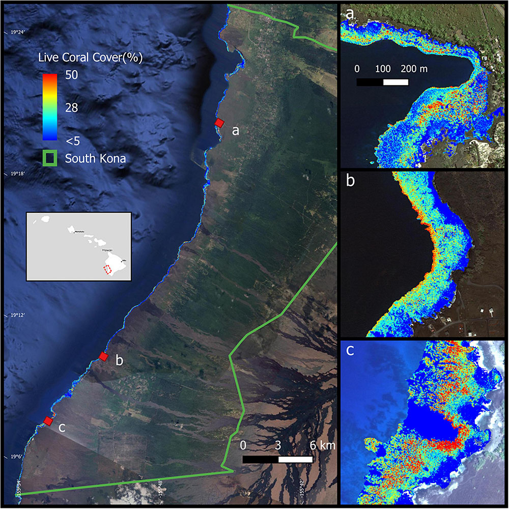
Figure 1. The location of South Kona District in green lines on the left, with live coral cover mapped along the coast (from Asner et al., 2020b). Example areas of live coral cover are shown at (a) H$\overline{\text{o}}$naunau Bay, (b) P$\overline{\text{a}}<cps:it>p</cps:it>\overline{\text{a}}$ Bay, and (c) Okoe-Kapua Bay. Background imagery retrieved from Google, ©2020 Digital Globe, ©2021 Maxar Technologies.

The South Kona District shoreline is dotted by large embayments including Kealakekua, H$\overline{\text{o}}$naunau, Ki‘ilae, Kipahoehoe, P$\overline{\text{a}}<cps:it>p</cps:it>\overline{\text{a}}$, Miloli‘i, Honomalino, Okoe, Kapu, and Manuk$\overline{\text{a}}$ bays. Other numerous coves and long stretches of non-embayments, along with coastal headlands, are common as well. Compared to other areas of Hawai‘i Island, South Kona District has fewer and less intensive areas of nutrient- or sediment-rich effluent from onshore disposal sites, golf courses or other land-based sources (Gove et al., 2016). This results in relatively clear waters with visibility often exceeding 30 m. Exceptions to this include two northern embayments of Kealakekua and H$\overline{\text{o}}$naunau, which can become turbid from runoff and/or high visitor traffic (Wedding et al., 2018). Physical oceanographic data indicate that the prevailing current is in the north-to-south direction and distinct areas and/or periods of upwelling are also common throughout the region (Gove et al., 2019).

Airborne Mapping of Benthic Variables

We used the Global Airborne Observatory (GAO), formerly known as Carnegie Airborne Observatory (Asner et al., 2012), to map a suite of benthic variables throughout the South Kona District. Water depth maps were created using a neural network model applied to the GAO imaging spectrometer (hyperspectral) reflectance data from campaigns in 2019 and 2020 as detailed in Asner et al. (2020a). The resulting depth maps have a spatial resolution of 2 m, and a depth range of 0–16 m (Asner et al., 2021), with a demonstrable accuracy comparable to estimates from other bathymetric studies (Asner et al., 2020a).

Because habitat complexity can strongly influence reef fish assemblages (Graham et al., 2015), we generated reef rugosity maps using a standard metric applied to the high-resolution water depth maps. We mapped two resolutions of rugosity using the surface-to-planar area methodology described in Asner et al. (2021): 2-m resolution maps of fine-scale rugosity and 6-m resolution maps of coarse-scale rugosity. Fine-scale rugosity captures high-frequency benthic surface variability caused by coral colonies, rocks and other features, whereas coarse-scale rugosity captures larger terrain features resulting from reef-scale geologic accretion and subsidence processes affecting wave forces and light regimes.

Finally, we used a computational deep learning model to estimate the percent cover of live coral, macroalgae, and sand from the same 2-m resolution imaging spectroscopy data across the study region (Asner et al., 2020b). From small-scale studies, live coral and macroalgal cover are often linked to habitat complexity, yet in prior studies we found that, across the full Hawaiian archipelago, the association between rugosity and live coral cover was not consistent between islands, and rugosity has a stronger link to many other factors tested (Asner et al., 2020b, 2021). Therefore, we included coral cover and habitat complexity separately. In sum, we derived benthic variables commonly known to influence fish populations (e.g., Gorospe et al., 2018): water depth, reef rugosity, and live coral cover, and we added macroalgal cover with the hypothesis that it could be associated with an increased presence of herbivorous fish.

Regional Stratification

We used an iterative, multi-stage process to determine the minimal set of mapped variables and the resulting minimal number of reef strata needed to meet three goals: (i) increase field survey efficiency, (ii) reduce field sampling costs, and (iii) ensure field sampling is geostatistically robust for upscaling to regional estimates of reef fish composition (Figure 2). In addition to our mapped benthic variables, our process started with a broad suite of input environmental variables (Supplementary Table 1 and Supplementary Figures 1, 2) known to affect reef fish biomass and diversity through ridge-to-reef impacts on water quality (Carlson et al., 2019), influences on human accessibility (Cinner et al., 2018), or direct impacts on fish habitat (Gorospe et al., 2018). Because the spatial resolution of many of these input maps was coarse compared to the GAO input maps, all maps were initially rescaled to 30-m resolution by pixel averaging for down-sampling or cubic-spline interpolation for upscaling. This reduced the data size and made the spatial variability of each of the considered variables more comparable.

FIGURE 2

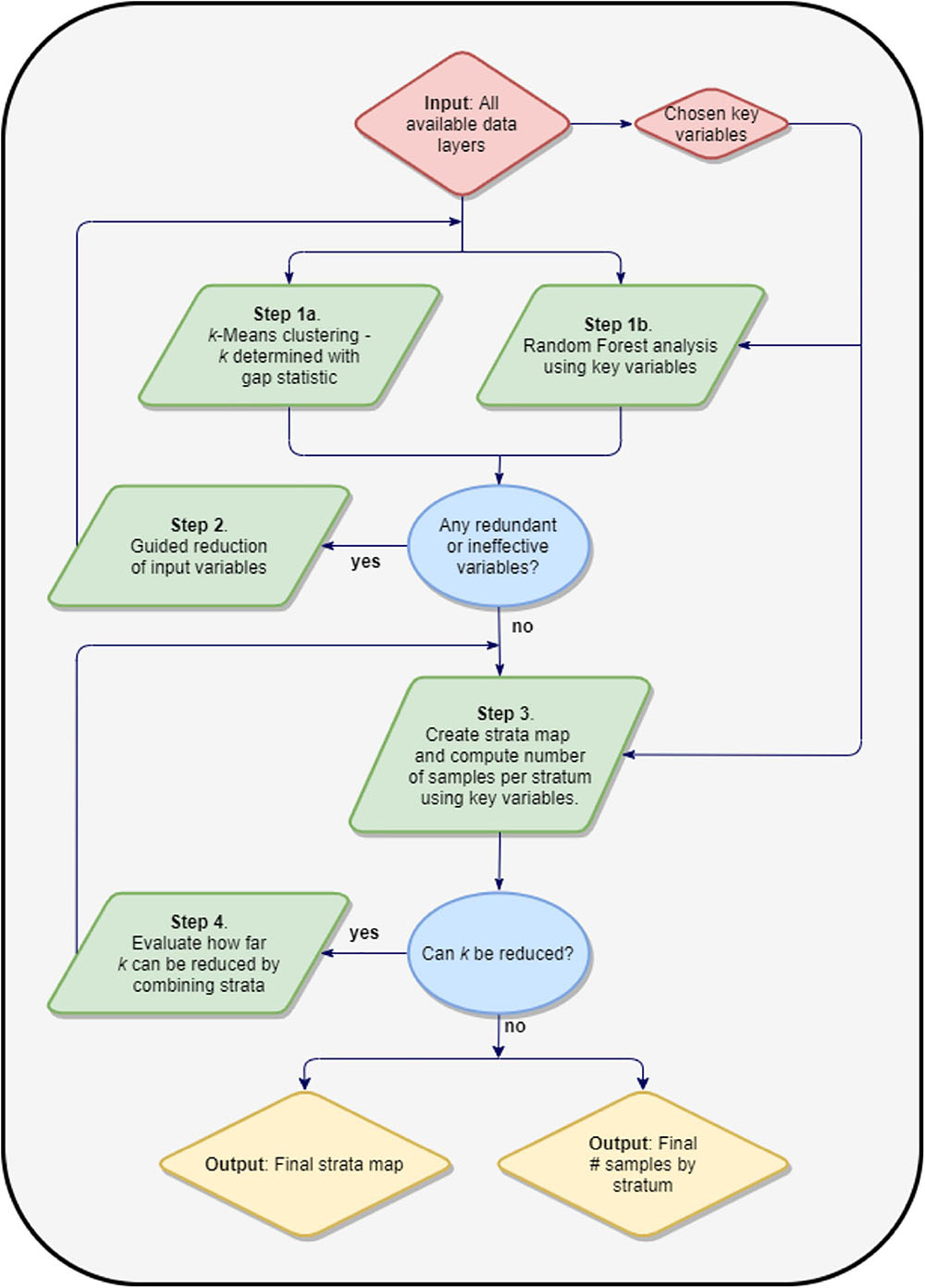
Figure 2. Overview of iterative geospatial clustering and stratification process for coral reefs.

The first step involved rescaling all input variables to a mean of 0 and a standard deviation of 1. Categorical variables needed to be converted to multiple columns of data using one-hot encoding or similar. A k-means clustering procedure (MacQueen, 1967) was used with k determined with the aid of the Gap statistic (Tibshirani et al., 2001). The resulting stratification map and means within each stratum informed subsequent steps. A separate Random Forest Machine Learning (RFML) model (Breiman, 2001) was run on the input dataset against designated “core” variables: live coral cover and rugosity, as they are known to correlate most strongly with fish biomass (e.g., Friedlander et al., 2007; Gorospe et al., 2018). A permutation-based importance measure for each input variable, along with a partial dependence plot for each variable, also informed the next step.

Using results from step one, we determined variables that met either of two conditions: (i) less than a 20% relative contribution to changing the overall explanatory performance of the model; or (ii) near zero variation between cluster-level means. The first condition indicates that the variable is too weakly correlated with the designated core variable to be of significance in the model. The second condition indicates that the variable does little to differentiate the habitat diversity within the survey region. When such variables were found, they were removed from the input dataset and the first step was repeated until all remaining input variables did not meet (i.e., were not screened out by) the two conditions above.

Upon completion of the two steps above, we generated a map of the k clusters by applying a k-means model to maps of the remaining input variables. These mapped clusters were treated as strata for a stratified random sampling scheme. We evaluated the number of field samples needed to satisfy the geospatial and ecological variation in the mapping variables under the given stratification using a standard methodology of allotting samples to an individual stratum based on its relative size and the standard deviation of core variable values within the stratum. This was done for each core variable by specifying a confidence interval level (α), and a maximum half-width of the confidence interval (x) as a percent of the core variable mean, and a table containing the within-stratum means (${\overline{Y}}_i$) and standard deviations (σ_i) for the core variable from the input map grouped by the levels in the strata map. By apportioning the field samples to each stratum (n_i) proportional to the area covered by that stratum (N_i), multiplied by stratum population standard deviation, σ_i, of the core variable within that stratum, i.e., n_i∝N_iσ_i, the optimal number of samples for the region (n) and the number computing a table containing the within-stratum means (${\overline{Y}}_i$) and standard deviations (σ_i) for the core variable from the input map grouped by the levels in the strata map. By apportioning the field samples to each stratum (n_i) proportional to the area covered by that stratum (N_i), multiplied by stratum population standard deviation, σ_i, of the core variable within that stratum, i.e., n_i∝N_iσ_i, the optimal number of samples for the region (n) and the number of samples per stratum were computed simultaneously using the formula:

$$n>\frac{z_{\mathrm{\alpha }}^2{\sum }_{i\in K}\frac{w_i{\mathrm{\sigma }}_i^2}{c_i}}{\left(x\overline{Y}/100\right)}$$

where:

$$c_i={\displaystyle \frac{N_i{\mathrm{\sigma }}_i}{{\sum }_{j\in K}{N}_j{\mathrm{\sigma }}_j}},c_i={\displaystyle \frac{N_i{\mathrm{\sigma }}_i}{{\sum }_{j\in K}{N}_j{\mathrm{\sigma }}_j}},$$

$$w_i={\displaystyle \frac{N_i}{N}},and{w}_i={\displaystyle \frac{N_i}{N}},and$$

$$n_i=ceil(c_{i}n)n_i=ceil(c_{i}n)$$

While too few strata will increase the number of field samples needed to obtain our desired level of confidence, numerous small, uncommon strata will make sampling within each stratum difficult and costly. We ran an analysis to investigate whether the number of strata could be further reduced by combining similar strata without significantly increasing the number of total field samples needed. Using the formula above, we assessed the increase in the minimum number of samples needed as individual strata were iteratively combined to generate a reduced number of strata by replacing the remaining next closest pair of existing strata on the dendrogram from the clustering procedure into one. At each step, the number of required samples was recomputed, and this was repeated until only one stratum remained. This approach indicated how many strata can be combined to reduce field costs without losing geostatistical robustness and efficiency.

At the conclusion of this process, the output consisted of a map of k strata across the study region, and the minimum number of field sites needed in each stratum to meet the desired uncertainty condition for each of the key variables. Doing so ensured that the field data could be upscaled in a geostatistically and ecologically robust manner. All modeling steps were carried out in the Python programming language, incorporating tools contained in the Scikit-learn package (Pedregosa et al., 2011).

Field-Based Fish Surveys

We used a restricted random selection process to identify suitable field site locations where transects would be established within each of the final strata from the procedure above. Our goal was to identify survey locations across both the North-South range and the available depth range of each stratum. Ideally, we aimed to locate all sites entirely within the area of their specified stratum. Such locations would be “pure,” i.e., all map pixels within 25 m × 15 m (our transect area) of each location would belong to the stratum. However, the spatial dimensions of some strata (too narrow, too sparse, etc.) precluded the identification of such a pure sample. To maximize purity of the field sites per stratum, we considered only pixels where surrounding area pixel purity was greater than a specified minimum of 75%. At the start of the iterative selection process for each stratum, we ran a 13 × 13 pixel moving window over the cluster map computing the pixel purity for each pixel in the strata map. If we did not find a sufficient number of suitable locations meeting the purity threshold, this threshold was reduced by 5% until a suitable number of sites was reached. Once a sample location was selected, we optimized the stratum purity of this sample by automatically adjusting the transect azimuth direction.

To keep the site locations from clustering too close together during the selection process, we used a weighted random sampling approach. All potential site locations were initially weighted equally. Higher weights increased the likelihood of selecting a given location as a site, where a weight of 0 disqualified that location. Each time a new sample location was chosen, the weight of all sample locations within 50 m of this selected location was set to zero, and weights between 50 and 300 m of the selected location were multiplied by 0.5. This greatly reduced site clustering, except in cases of extremely sparse strata.

As a secondary criterion, we also wanted site locations to represent the full range of depth of each stratum. During the iterative site selection process, we split the total area of each stratum into three equal parts to represent shallow (0–5 m), medium (5–10 m) and deeper (10–16 m) depths based on percentiles of the pixel depth values, and allotted site locations between these depth classes as uniformly as possible. Overall, our site selection process yielded 117 sites across 18 strata (Supplementary Figure 3; see details on stratification output in section “Results”).

We assessed reef fish biomass and biodiversity using a standard 25 m × 5 m underwater visual belt transect survey method (Brock, 1982; Friedlander et al., 2006, Friedlander et al., 2006, 2007). Underwater visual census (UVC) surveys are a practical diver-based approach to capture the abundance, biomass, and diversity of reef fishes in shallow reef environments (Brock, 1954; Samoilys and Carlos, 2000; Friedlander et al., 2018). Studies implementing UVC surveys have used several variants of this method which include stationary point counts (Campbell, 1986; Heenan et al., 2014) and visual belt transects (Halford and Thompson, 1994; Friedlander et al., 2006). Each of these variants of UVC surveys collect comparable data but have caveats due to restrictions in their ability to detect certain cryptic species as well as their spatial and temporal coverage of reef environments (Samoilys and Carlos, 2000; Edgar et al., 2004; Fernández et al., 2021). However, for capturing general reef fish populations densities, UVC surveys are low cost, easy to implement, and malleable to different research and management needs.

At each site, two divers each completed a transect approximately 10 m apart, which were then averaged during data analysis. We identified all fish on the transect to species level, and visually estimated the size of fish by total length, binning fish into five cm slots up to 25 cm, and to the nearest cm for fish greater than 25 cm. We swam across the transects at a constant rate, with an average survey time of 15 min per transect.

Biomass (kg ha^–1) was estimated using size and weight values from Fishbase¹. Species were grouped by trophic structure as three sub-groups: grazer, browser, and scraper. Trophic groups were generated from pre-existing groups following Heenan et al. (2016) as well from unpublished data from the Division of Aquatic Resources, State of Hawai‘i. We estimated species richness as the number of species present as well as the Shannon diversity (H) index at each site (Shannon, 1948). The behavior, mobility, and schooling assemblage habits of certain fishes, such as those in the families Acanthuridae, Scaridae, Mullidae, and Lutjanidae, may bias upscaled map data by creating higher frequency biomass hotspots or anomalies in high resolution map data (Donovan et al., 2018). The design of UVC surveys to census the biomass and diversity of fishes does not incorporate fish assemblages that are temporary, haphazard, and non-uniformly distributed across a reef. As a result, temporary schooling fish cause data bias when upscaling to high resolution maps (Donovan et al., 2018). To account for large schooling fish and fish biomass anomalies that overestimate or bias map data, sites that had both schools of 20 fish or more and a biomass over 500 kg ha^–1 were replaced by the average biomass for that species that occurred in the stratum for the site. This was applied to data from 12 of the 117 sites, with each site only needing one replacement. For these 12 sites, species that displayed schooling behavior were Acanthurus leucopareius (n = 5; stratum 5, 6, 9), Acanthurus blochii (n = 1; stratum 15), Decapterus macarellus (n = 1; stratum 10), Lutjanus kasmira (n = 1; stratum 5), Mulloidichthys flavolineatus (n = 1; stratum 1), Mulloidichthys vanicolensis (n = 1; stratum 14), Naso lituratus (n = 1; stratum 16), and Scarus psittacus (n = 1; stratum 1). An example of this replacement was for a school of S. psittacus at a site in which a school of 245 fish with a biomass of 2900 kg ha^–1 was present. This schooling behavior caused extreme biomass anomalies in the map data and overestimated S. psittacus biomass, and thus was replaced by the average biomass for its stratum of 328 kg ha^–1. Large fishes that were rare, had high biomass, and were expected to have high mobility such as sharks and rays, were also removed from the data. We recognize the limitations of this averaging approach for some large schools of migratory fish. As a result, one can view this study as being focused on fish with smaller home ranges. Meanwhile, until new methods for more accurately measuring large schools with large home ranges are developed, this error will remain inherent to all transect-based field survey approaches. We feel that the stratum-averaging is a reasonable interim solution.

Regional Upscaling

Machine learning models were used to upscale the field data into South Kona regional maps. For each of the six biomass (total, grazer, browser, and scraper) and biodiversity (richness, Shannon diversity) values computed from transects, we built a RFML regression model trained with data collected from the 117 field sites matched with data from the full maps of the input variables that went into the final stratification process defined above.

To build a training dataset, we collected input map data from all 2 m × 2 m pixels falling within the mapped transect survey area of each field site and treated each of these pixels as an independent observation for the purpose of model training. All pixel observations for each field site were also assigned the transect-derived values of the response variables (fish biomass and diversity) from that field site. After discarding pixels with missing or invalid data in any of the input layers, this resulted in a dataset of 14,896 observations across the 117 field sites visited in the field (Supplementary Figure 3). A RFML model training requires specification of a few configuration parameters, and these parameters can affect the overall fit of the model. Thus, for each response variable the optimal configuration settings were found by fitting the model using a five-fold cross-validation approach across all combinations of the following grid of parameters: the number of regression trees in the RFML model (possibilities were 50, 75, 100, 250), the maximum branching depth (2 or 3 deep), and the minimum number of samples needed to split a node within each tree (2, 5, 10, or 20). The combination that gave the best fit, determined by minimal mean squared error using a cross-validation procedure was considered optimal.

The next step was to apply fitted RFML models to the input maps to derive estimates of fish biomass and biodiversity in each pixel in the input maps. The regional maps were made using a model averaging approach to further reduce the influence of high values measured at individual field sites. With this approach, the training data were grouped by field site and split into 10 equally sized parts. For each of the 10 parts, a model was fit with the previously determined optimal parameter settings using data from the other nine parts of the training data. Maps were produced by applying each of the 10 models to the full South Kona region input map pixel values, and the final output pixel value was taken as the average of these 10 predicted values. This 10-part process was performed for each of the six biomass and biodiversity output values.

Rarefaction Analysis to Minimize Number of Field Transects

After completing the analysis of the field transects and upscaling the results to region-wide maps, we assessed the degree to which the results could be obtained from fewer field sites. We assessed the effects of reducing the sampling sites on both point estimates of region-wide averages computed directly on the field site transect values and on the upscaled maps created using models built with the field sites used as training data. In both cases, we iteratively removed one site from each stratum with the minimal number of transects per stratum being one. The reduction was repeated with up to 18 transects removed for each iteration until each stratum had only one site remaining. This resulted in nine iterations with 99, 82, 65, 50, 38, 29, 24, 20, and 18 field sites used in total, and the statistics from each iteration were quantitatively compared to our nominal 117-site sampling approach.

To assess the effect of this reduction scheme on locational estimates of region-wide averages, we used a bootstrap approach, where at each iteration, the required number of field transects was selected at random with replacement from the full number of available transects for the given stratum. This simulates a full new field survey performed under the same design and was carried out for 30 permutations in each iteration, and the region-wide estimate of mean was recomputed for each permutation. An estimate of the standard error in the overall regional mean could be achieved using the standard deviation of the 30 bootstrap means for the given iteration, and a coefficient of variation (CV) was computed by dividing the estimated standard error by the mean of the permutation means across all 30 permutations. In this way, we could compute the increase in uncertainty as we reduce the overall sample size.

Because of the large computational requirements needed for the RFML models, the bootstrap approach was done with 10 permutations rather than 30 for assessing the effect of reduced sample sizes on upscaled map outputs. Here, the upscaling process, including full model training, was run to the point of map output creation for each of the 10 bootstrap permutations. Then, across the 10 permutations for each variable and iteration, we computed CV for each individual map pixel and for the regional average. This allowed us to examine the effects of site density reduction on map quality.

Results

Regional Stratification

For the South Kona study region, the initial gap-statistical analysis (step-1a of Figure 2) using the full suite of input variables (Supplementary Table 1) suggested up to 38 strata or benthic classes were needed to define the environmental and habitat conditions of all reefs (Supplementary Figure 4). However, the close relatedness of many of these strata suggested that several could be combined (Supplementary Figure 5).

Random Forest Machine Learning analysis of the environmental variables (Supplementary Table 1) indicated that a subset of these variables strongly predicted the location of two core habitat variables: live coral cover and fine-scale reef rugosity (Figure 3). Cross-validation estimates of R² for the RFML models were 0.82 and 0.41 for live coral cover and fine-scale reef rugosity, respectively. UTM Northing (equivalent to latitude), macroalgal cover and water depth were the principal determinants of live coral cover throughout the South Kona District. Fine-scale reef rugosity was determined primarily by UTM Northing, depth and reef curvature. Other variables contributed less than 20% to overall model performance and were removed from subsequent analyses.

FIGURE 3

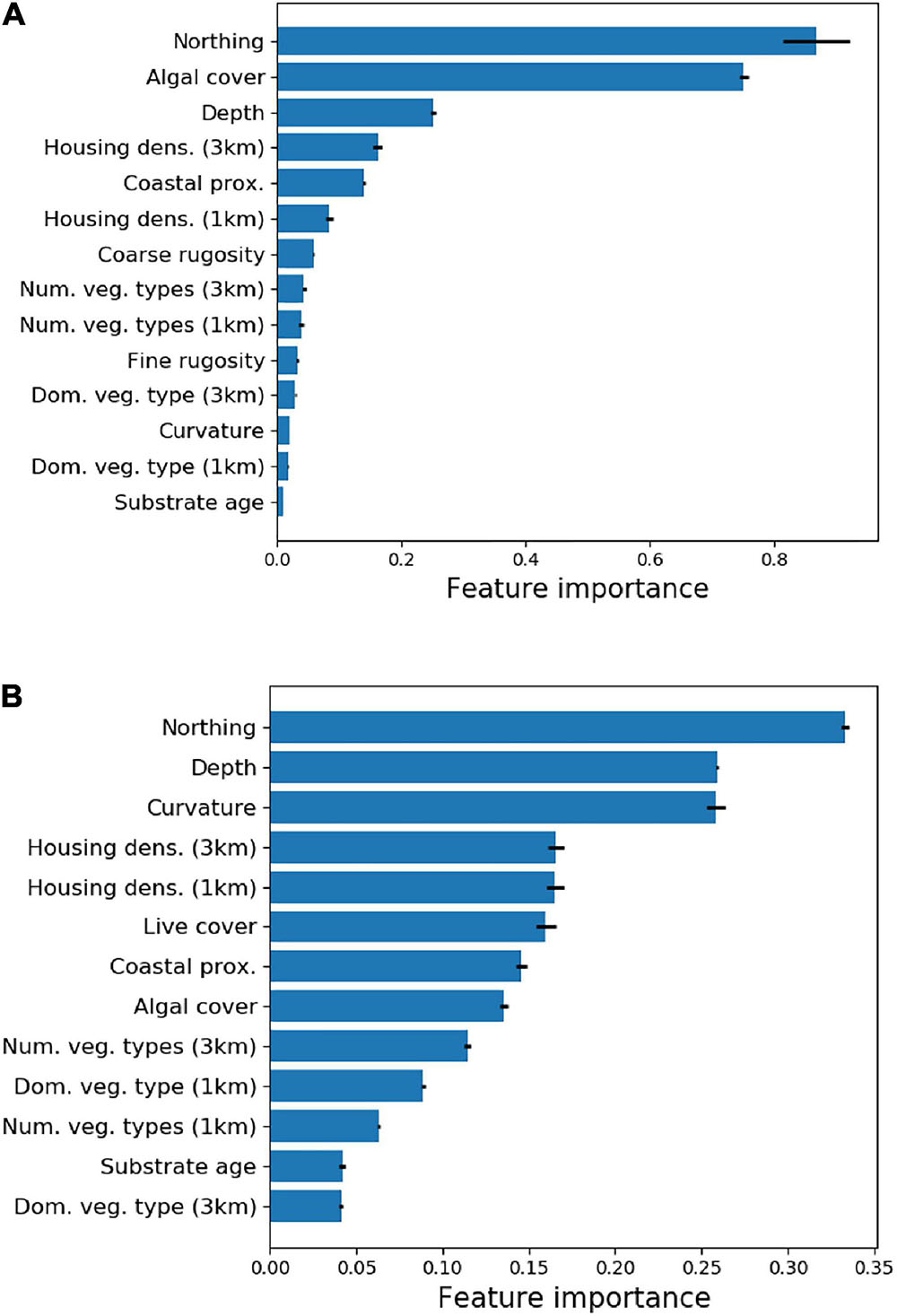
Figure 3. Relative importance of regional input variables (see Supplementary Table 1) on mapped (A) live coral cover and (B) fine-scale rugosity.

Successive iteration through analysis steps 1 and 2 (Figure 2) resulted in a dataset consisting of the following final stratification variables: UTM northing, water depth, reef curvature, fine-scale reef rugosity, live coral cover, and macroalgal cover. For the final stratification, we increased the spatial resolution of selected input maps to 2 m, the native resolution of the GAO input maps, to provide finer granularity in the resulting classification map. The number of remaining strata after this final iteration was 18 (Figure 4), or less than half of the 38 original strata (Supplementary Figure 5).

FIGURE 4

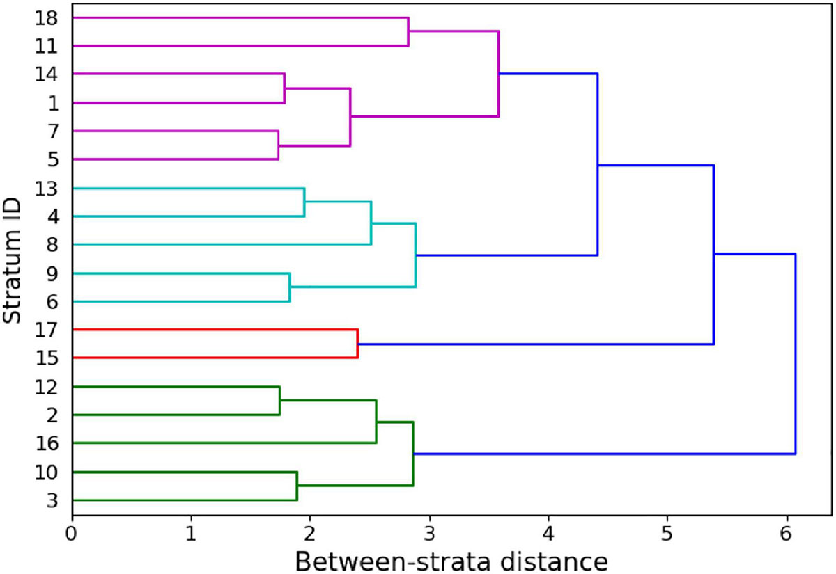
Figure 4. Dendrogram of the between-strata Euclidean distance within the reduced input set yielding 18 strata in the last iteration of Step 1 (Figure 2).

Within the final 18 strata, the number of field sites needed to meet our goal of a 95% confidence interval ranging only ±10% of each key variable mean was 117 and 35 if regional upscaling is based on live coral cover or fine-scale rugosity, respectively. Greater spatial variability in live coral cover generated the more stringent requirement of 117 field sites compared to fine-scale rugosity.

The 117 field sites were optimally apportioned based on stratified-random design using c_i defined above, which considers variation in live coral cover within each of the 18 strata (Table 1). For example, stratum 10, which covers a moderate level of reef area, but relatively little geospatial variation in live coral cover (SD = 0.04), required just four sampling transects randomly located anywhere within the bounds of the stratum. In contrast, stratum 7 covers more area and harbors high variation in live coral cover (SD = 0.09), thereby requiring nine sampling transects to capture sufficient variation in fish habitat (Table 1).

TABLE 1

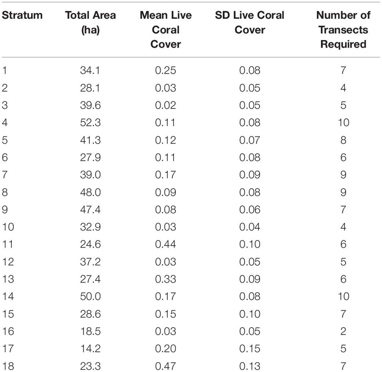
Table 1. Minimum number of field sampling transects required for each of the 18 mapping reef strata based on the stratum size and within-stratum standard deviation of live coral cover.

Investigation of whether a reduction in the number of strata was possible without reducing efficiency revealed a sharp increase in the number of sampling sites needed to meet uncertainty goals with anything less than 18 strata (Figure 5). Reducing all the way down to just one stratum increased the total number of transects needed for live coral-based sampling by nearly 50%. Notably, using one stratum is equivalent to simple random sampling along the entire South Kona District coast, and 379 samples for live coral cover and 106 samples for fine-scale rugosity would have been needed to meet the uncertainty goals for these habitat variables. The associated increase in geostatistical sampling efficiency with 18 strata was therefore 72% (to n = 117) and 67% (to n = 35), respectively, for live coral- and rugosity-based sampling. The final stratification map of the 18 distinct reef classes is shown in Figure 6. Inspection of these maps suggested three broad regional-scale groups of reef habitat (Figures 6a,b vs. Figures 6c,d vs. Figures 6f–h), which are driven by a combination of latitude (climate), substrate age and thus reef accretion stage, and similar large-scale factors. Within these groupings, local-scale variability in live coral and algal cover, depth, and rugosity sort habitat distributions within and among strata (Figure 3).

FIGURE 5

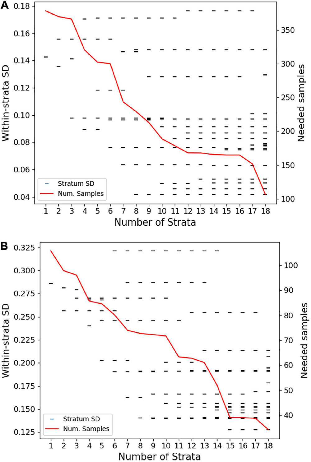
Figure 5. Sensitivity of the number of field-based transects (samples) needed to meet regional uncertainty criteria as the number of strata are increased from 1 to 18 based on regional variation in (A) live coral cover and (B) fine-scale reef rugosity. Tick marks indicate the within-stratum standard deviation or sampling error predicted when treating South Kona as one stratum (k = 1) to the 18 final strata based on the entire analysis. The red line indicates the total number of field-based transects (samples) required regionally at different levels of stratification (1–18), resulting in (A) 117 transects based on live coral and (B) 35 transects based on fine-scale reef rugosity.

FIGURE 6

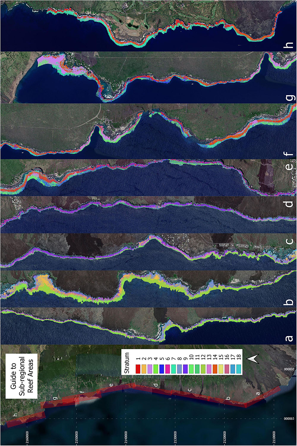
Figure 6. Final 18-stratum map of coral reef conditions for the coast of South Kona District. The far left panel indicates the location of each sub-regional zoom image (a–h) shown in the remaining panels. Each color indicates the location of each ecological stratum in the reef system. Background imagery retrieved from Google, ©2021 Maxar Technologies.

Field Results

Field surveys at the 117 sites in the 18 mapped reef strata yielded a total of 138 fish species throughout the South Kona study region. Average species richness was 35 species per site and the mean Shannon index was 2.15 per site (Supplementary Figure 6). Both distributions were skewed to the right.

Total fish biomass averaged 1295 kg ha^–1 in the South Kona region. Grazers were the dominant trophic group averaging 421 kg ha^–1, followed by browsers at 247 kg ha^–1, and scrapers at 174 kg ha^–1. These averages were determined as a weighted average of the stratum-level means, where weighting was based on stratum area. Stratum 4 (0.11 ± 0.08 live coral cover) had the highest biomass as well as the highest species richness, whereas stratum 5 (0.12 ± 0.07 live coral cover) had the highest diversity and equal species richness to stratum 4 (Table 2). Stratum 2 (0.03 ± 0.05 live coral cover) had the lowest biomass, diversity, and species richness (Table 2). The top three fish in terms of average biomass were N. lituratus, Scarus rubroviolaceus, and Acanthurus olivaceus.

TABLE 2

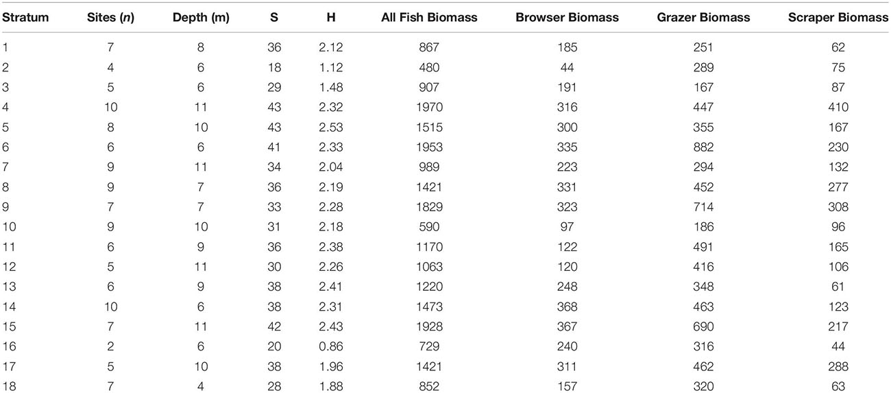
Table 2. Mean field-based results by map stratum of water depth and species richness (S), Shannon diversity (H), and biomass (kg ha^–1) of all fish, as well as biomass for browser, grazer, and scraper trophic groups.

Upscaled Fish Biomass and Biodiversity Maps

The optimal parameter settings and model fit quality varied considerably between response variables, with R² ranging from 0.32 to 0.38 for the biomass outputs and 0.54 to 0.58 for the biodiversity outputs (Supplementary Table 2). The resulting upscaled biomass maps each covered a total of 706 ha of South Kona reef to 16 m water depth (Supplementary Figures 7–10). A zoomed in example from Honomalino Bay is shown to demonstrate spatial detail (Figure 7). These maps represent our best estimates of spatial patterns of biomass abundance for all fish species as well as for three key fish trophic groups: browsers, scrapers, and grazers, for the entire South Kona reef ecosystem (Supplementary Figures 7–10). Estimated biomass of the different trophic groups was 541,400 kg for all species, 106,052 kg for browsers, 184,399 kg for grazers, and 66,293 kg for scrapers. Species richness per site in mapped data peaked at 30–35 species per stratum, and the two maps of fish species diversity showed strong inter-map agreement, with the map of total species count displaying greater variability between low and medium to high values (zoom example: Figure 8, all data: Supplementary Figures 11, 12).

FIGURE 7

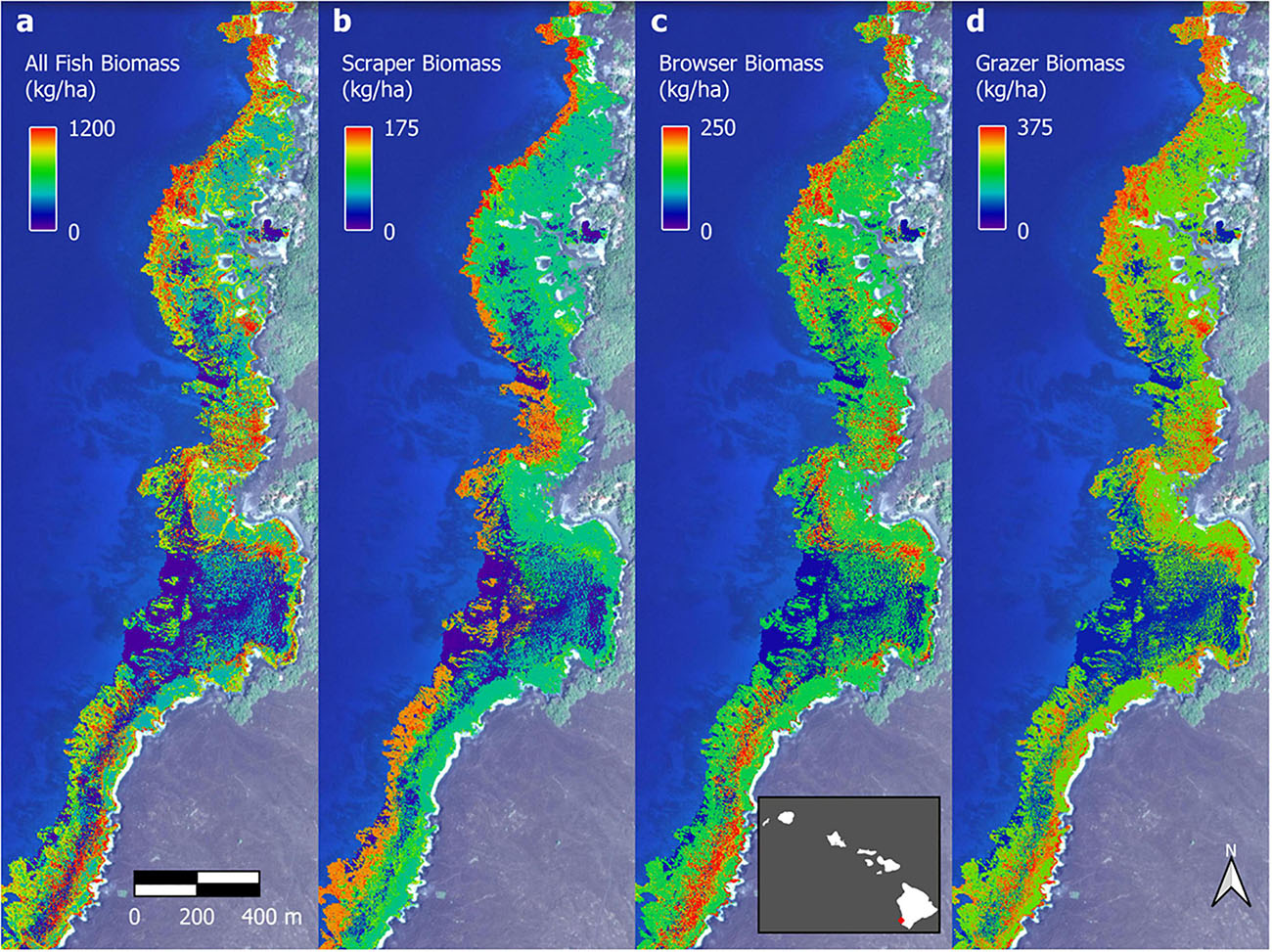
Figure 7. Example fish biomass maps of Honomalino Bay for (a) all fish, and for fish classified as: (b) scrapers, (c) browsers, and (d) grazers. Distributional pattern differences can be seen between the different trophic groups, especially across depth gradients. Full maps in Supplementary Figures 7–10. Background imagery retrieved from Google, ©2021 Maxar Technologies.

FIGURE 8

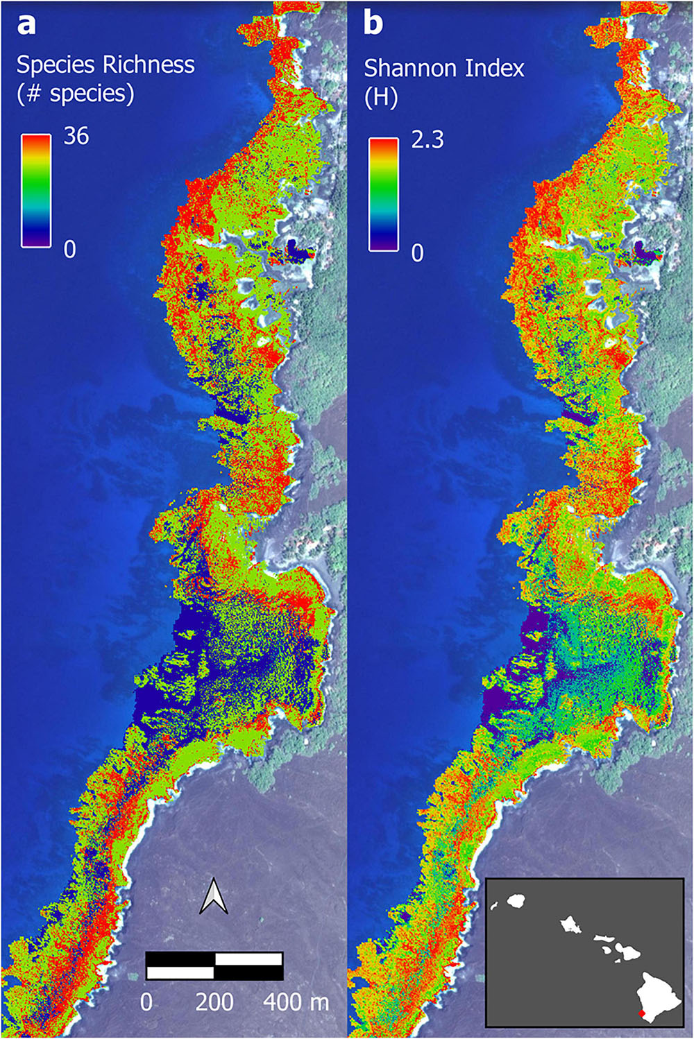
Figure 8. Example of upscaled biodiversity maps of Honomalino Bay using (a) species richness and (b) Shannon diversity index. Full maps in Supplementary Figures 11, 12. Background imagery retrieved from Google, ©2021 Maxar Technologies.

Distributions of mapped fish biomass varied by fish functional group and depth (Figure 9). For all fish species, the distribution of high and low biomass values was similar in shape between depth classes of 0–5 m, 5–10 m, and 10–16 m, with all depths showing higher numbers of low biomass species (skew to the left). However, for the scraper fish group, higher values of biomass were most abundant in deeper water (10–16 m). For species richness and Shannon index, there was skew to the right, with a high number of sites showing relatively high diversity. This pattern occurred across all depth classes.

FIGURE 9

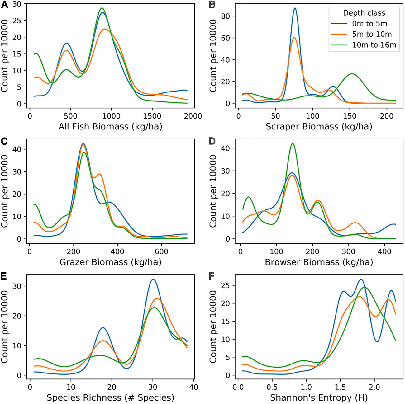
Figure 9. Distribution of mapped biomass of: (A) All fish, and for fish classified as (B) scrapers, (C) browsers, and (D) grazers, as well as two measures of biodiversity: (E) species richness and (F) Shannon index, as distributed in benthic depths 0–5 m, 5–10 m, and 10–16 m across the South Kona District.

Site Rarefaction Analysis

We assessed the sensitivity of the stratified-random sampling approach to decreasing densities of field survey sites. The data from the 117 field sites were reduced by one site per stratum until a minimum of one site was retained in each stratum (n = 18 total sites). The coefficient of variation (CV) was calculated at each stage of rarefaction to determine different levels of uncertainty based on field site density (Figure 10). Because different monitoring programs can accommodate different levels of uncertainty, we present the trends without interpretation of the minimum number of field sites required. However, we did find that, in the South Kona region, it takes far fewer sites to monitor fish diversity (richness, Shannon index) than it does to monitor fish biomass. For example, just 45 sites are required to monitor species richness along the 60.5 km reef at an uncertainty level of 5% CV (Figure 10a). In contrast, 80–90 sites are required to meet a 5% CV threshold for all fish biomass as well as fish biomass for each of our trophic groups (Figure 10b). The difference in site requirements for diversity vs. biomass is due to the relatively well-mixed communities of species found within the study depth range of 1–16 m. In contrast, biomass is much more variable within and across habitats.

FIGURE 10

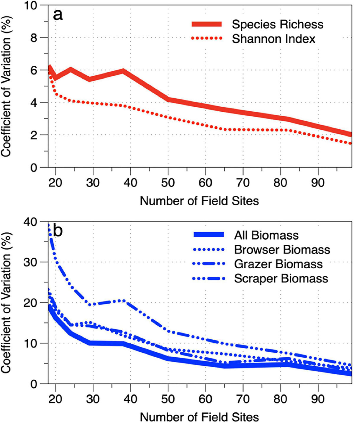
Figure 10. Reduction in bootstrap coefficient of variation (CV) while increasing the number field sites used in the stratum-level mean estimates of (a) fish species diversity and (b) fish biomass values under the stratified-random sampling scheme. These trends indicate our ability to capture the true mean value of each of the 18 strata using field measurements.

We also considered the effects of decreasing field site density on the average regional-scale diversity and biomass of the South Kona reef ecosystem. This calculation was made using a bootstrap approach by resampling the field transects within each stratum 10 times at several levels of site density reduction from 117 to 18 sites and running the regional upscaling procedure for each of the 10 permutations. The uncertainty for a given map value for each of the biomass and diversity indicators was then calculated using the coefficient of variation (CV) across the values obtained from the 10 permutations. This was first done for the mean pixel value from each map. When the number of field sites was reduced by one site per stratum, map-level pixel uncertainties increased for each of the biomass and diversity indicators (Supplementary Figure 13). Similar to the field-site results (Figure 10), diversity indicators were more stable at an uncertainty of about 5% as field-site density decreased from 117 to 40 sites. Thereafter, diversity indicators became unstable, with increasing uncertainty peaking at 13% with only 18 field sites incorporated into the maps.

Average regional-scale fish biomass estimates proved to be far more sensitive to the number of field sites used for upscaling (Supplementary Figure 13). Biomass of all fish averaged 10% uncertainty as field site density was decreased from 117 to 50 sites. Thereafter, regional-level uncertainties for all fish combined increased to 15% and eventually to 30% at a field sampling density of just 18 sites, or one site per mapping stratum. However, grazer and especially scraper biomass was much more sensitive to decreasing sites, with the latter peaking at 30–50% uncertainty when fewer than 30 field sites were used in the regional mapping.

The process of increasing uncertainty with decreasing field-site density resulted in a loss of map fidelity. In an example from Honomalino Bay, Supplementary Figure 14 was generated using all 117 field sites, and each panel thereafter shows the same map after reducing the number of sites per regional stratum by one site to a minimum of 18 sites region-wide. Supplementary Figure 14J was created with the minimum 18 sites, and shows the erroneous and dichotomous nature of the resulting all-fish biomass map, which depicts strong differences between shallow and deep water habitats.

Finally, we analyzed the sensitivity of individual biomass pixels in the maps to decreasing field-based sampling and calibration. For each pixel, we determined whether the CV became unstable using an iterative approach that tracked the mean and standard deviation of every pixel CV value with progressively fewer and fewer regional-scale field site densities (n = 117 to 18). When the CV value of a pixel increased more than 1.25 standard deviations from its previous value, then the number of samples before this occurrence was recorded and the analysis was halted for that pixel. By applying this to all pixels in the South Kona region, we mapped the spatial pattern of uncertainty in the output maps caused by reduced field site data collections. An example of this process is shown in Figure 11 for Honomalino and Miloli‘i Bays, depicting the pixel-by-pixel minimum field site density required for South Kona to prevent instability in the mapped fish biomass results. Brighter pixels indicate areas of reef in which greater field-site sample sizes are needed in order to remain statistically robust for regional monitoring. Areas of low field-sample needs (purple-blue) are dominated by stretches of open sand; areas of moderate field-sample needs (blue-green) are mixed sand and rock surfaces; and areas of high field-sample needs (yellow-red) are coral-rock mixed benthic surfaces. A complete coverage of the South Kona reef ecosystem for all-fish biomass is provided in Supplementary Figure 15, which highlights the large stretches of reef that become statistically unstable for monitoring with too few field sites.

FIGURE 11

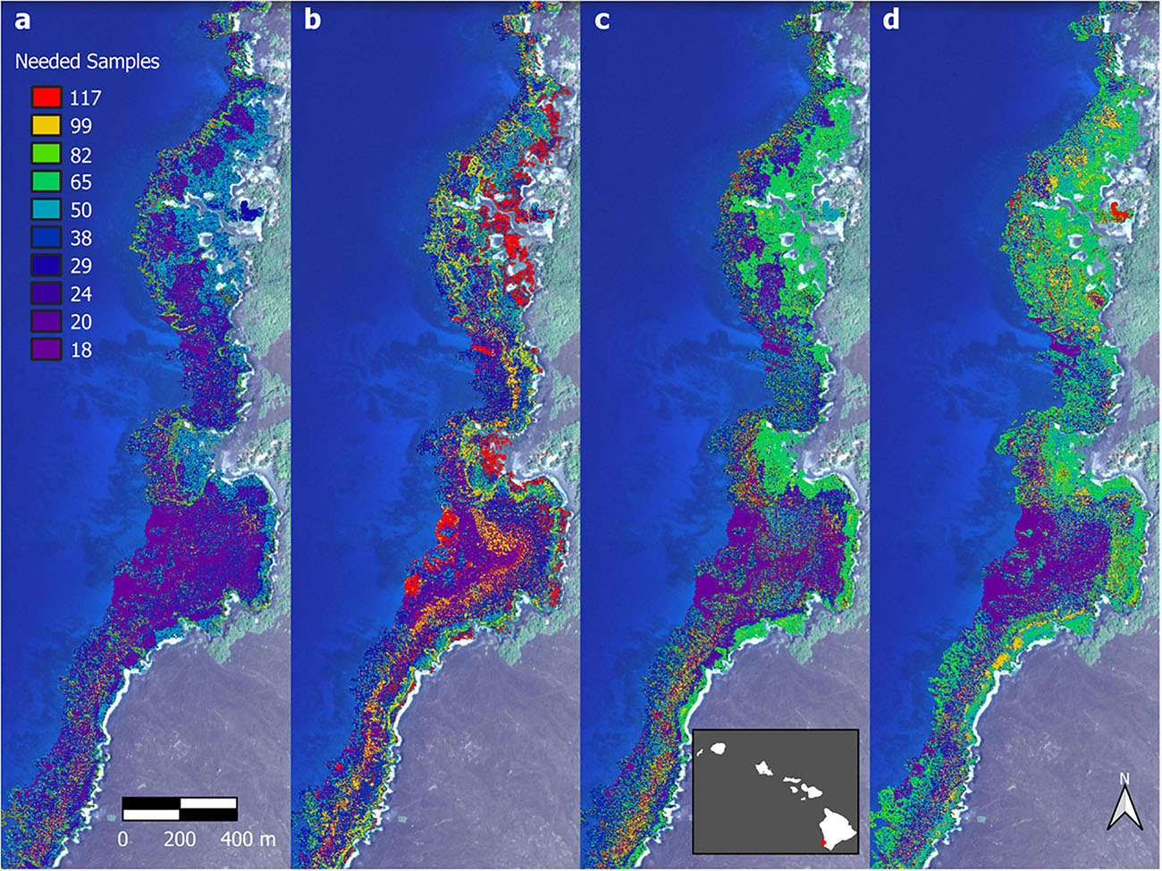
Figure 11. Loss in mapped spatial structure of (a) total fish biomass, (b) scrapers, (c) browsers, and (d) grazers that results from a reduction in the number of field sites used in the upscaling process. Background imagery retrieved from Google, ©2021 Maxar Technologies.

Discussion

We developed, implemented, and assessed a method for high-resolution mapping of fish diversity and biomass using a combination of new airborne remote sensing, freely available land-based maps, and in-situ field surveys. Across more than 60 km of the South Kona reef ecosystem of Hawai‘i Island, the approach yielded spatially explicit estimates of fish diversity and biomass, along with comprehensively analyzed uncertainties based on field sampling density. The habitat mapping component of the approach relied on new operational benthic products derived from the GAO (Asner et al., 2020b, 2021). In combination, these and complementary coastal land and climate maps facilitated a large-scale, high-resolution reef stratification to direct field surveys in an ecologically robust geospatial pattern. Whereas traditional fish survey methods have used stratified random sampling to determine survey locations, most have not incorporated detailed habitat variability (see review by Mellin et al., 2009). The method developed and tested here allows an optimization of both the number and distribution of field surveys to provide a more accurate representation of fish populations.

Any socio-ecological stratification process involves trade-offs between mapped environmental detail, derivation of input maps to meet monitoring goals, and the time and cost of field sampling. In our case, we sought to randomly sample reef fish diversity and biomass in a manner that is most robust in scaling up to spatially explicit maps and regional total stock estimates. To do so, we focused on factors known to affect fish composition and stocks, thereby folding in numerous potential benthic, terrestrial and human factors. Out of the initial set of potential factors, our analyses suggested that live coral cover, macroalgal cover, water depth, fine-scale rugosity, and latitude (as UTM northing) were most important in defining habitat. In South Kona, latitude is a proxy for the north-south precipitation gradient that occurs along the coast (Giambelluca et al., 2013). Based on these reduced inputs, a set of 18 regional reef strata emerged from classification to apply in subsequent random, field-based sampling. Critically, the number of field sites per stratum was based on the variability of the two primary mapped drivers of fish habitat: live coral cover and fine-scale rugosity. This is important because it took into account habitat variability, rather than simply the average conditions of habitat in each reef class. This, in turn, facilitated quantitative upscaling of the field data based on actual habitat variability.

The resulting regional maps of fish diversity and biomass yielded numerous findings. First, fish diversity, both in terms of species richness and Shannon index, is spatially more uniform than fish biomass throughout the South Kona reef ecosystem. These results are consistent with recent findings from H$\overline{\text{a}}$’ena, Kaua’i, where overall species richness, diversity, and assemblage composition did not significantly differ inside and outside of a Community-Based Subsistence Fishing Area (Weible et al., 2021). Greater variability in fish biomass relative to diversity suggests that biomass is more sensitive to habitat factors regulating the amount of fish per unit reef area. However, biomass variability could also be due to spatial variability in fishing pressure, which is very high in some areas of South Kona (Foo et al., 2020). Additionally, the field-based richness surveys yielded an average of 35 species per site, whereas upscaled, map-based richness peaked at 30–35 species per stratum and was often much lower. The map-based results take into account habitat variability and its relationship to fish diversity as calibrated via the field study, strongly suggesting that not all habitats support similar levels of fish diversity in South Kona, a finding that could be missed using field surveys alone.

A second set of findings indicated that total fish biomass was often lowest in embayments, owing to larger patches of open sand habitat that contain fewer fish as well as the possible effects of increased fishing accessibility in bays (Friedlander et al., 2018). Field data indicated an average biomass of all fish of 1295 kg ha^–1, but upscaled and mapped-based biomass averaged about 800 kg ha^–1 (Figure 9A). Similar to the biodiversity results, the lower map-based biomass compared to field data was due to the relative sparseness of suitable fish habitat throughout the South Kona reef ecosystem, relative to habitats represented in the field-based calibration sites. Notably, regional biomass estimates of scrapers, grazers, and browsers averaged 60, 200, and 100 kg ha^–1, respectively (Figures 9B–D), compared to field values of 174, 421, and 247 kg ha^–1, again highlighting the fact that habitat variability can cause over-estimates of biomass using field sites alone.

We also assessed the sensitivity of our method to a reduction in the total number of field sites deployed to calculate the minimum number of transects that could have been used to achieve similar results. We first undertook a stringent 117-site sampling of the South Kona coast to generate diversity and biomass estimates at a 95% confidence level. Doing so provided the strong statistical power for establishing the spatial pattern, which greatly affects our ability to detect future change. To increase monitoring efficiency, we then artificially reduced the number of field sites and reanalyzed the results at different reef aggregation levels. First, we found that reducing the number of sites had a moderate effect on estimates of fish species richness and Shannon diversity (Figure 10a). Specifically, reductions from 117 sites to 18 sites (or one site per mapped habitat) only increased the coefficient of variation (CV) in mean stratum-weighted diversity estimates by 6%. This again points to the relative evenness of species distributions throughout the South Kona reef ecosystem. In stark contrast, reduction of field sample density from 117 to 18 sites resulted in a 20–40% increase in total fish biomass CV, meaning that 18 surveys would not allow a trend in fish populations to be detected accurately over time. South Kona requires no less than 40 sites to maintain an uncertainty of 10% CV for total fish biomass monitoring. However, this finding is also strongly dependent upon fish trophic group. For the deeper and more sparsely distributed scraper fish group, 70 sites are needed just to meet the 10% CV threshold (Figure 10b). The methods presented here can be adapted to the specific group of fish being monitored.

At the regional level, decreasing numbers of field sampling sites resulted in average uncertainties of up to 30% for total fish biomass and 50% for scraper biomass (Supplementary Figure 13). When viewed in mapped format, these increasing uncertainties are non-uniform, with hotspots of error emerging in complex geospatial patterns associated with benthic habitat variability (Figure 11 and Supplementary Figure 15). These findings strongly suggest that the negative impacts of undersampling should be considered on a ecologically explicit basis.

This first effort focused on 60 km of coastline along Hawai‘i Island, with the advantage of good boat and diver access combined with high-resolution airborne hyperspectral and regional ancillary map data. While the South Kona region is ecologically variable, with more than 10 embayments, numerous headlands, and long stretches of variable reef morphology, even this region does not represent the extreme reef habitat variability found across the Main Hawaiian Islands, which is mediated by island age, geologic substrate, subsidence, physical oceanographic conditions and other factors. Scaling up our approach to the main Hawaiian Islands is readily possible given that we have the same benthic mapping data for the entire archipelago, yet doing so may yield an untenable number of reef strata for field sampling unless more work is done to further assess relationships between habitat complexity, benthic composition, and fish communities at the scale of the entire archipelago. This presents a challenge that can be addressed via iterative map-based analyses and field-based surveys until the broader reef-fish relationships are better quantified. In parallel to the Hawai‘i roll-out of this approach, there are other regions of the world where fish survey data exist in sufficient quality and geospatial density to further test the upscaling approach presented here. This has already been undertaken using multi-spectral satellite data on benthic habitat composition and bathymetry (Purkis et al., 2008; Knudby et al., 2011). Adding new airborne and forthcoming spaceborne imaging spectrometer data could increase the fidelity of these efforts through more detailed mapping of coral and non-coral dominated habitats.

We showed that high-resolution benthic mapping can be combined with stratified-random field sampling to generate spatially explicit estimates of fish diversity and biomass over large ecologically complex reef systems. The approach presented here can be used for any population, community, or ecosystem-level study that relies on reef habitat as defined by the types of benthic, terrestrial, and human factors mapped here, and could be considered when designing and implementing new marine monitoring programs or increasing the efficiency of existing programs. Other upscaling methods could be used, and there are many available, but we chose to proceed with a common type of machine learning (RFML) due to its flexibility, lack of assumptions regarding input data, and the available tools for avoiding overfitting. Similarly, other remote sensing technology, such as high-resolution laser scanning and radar for additional information on benthic and sea surface structure, could yield additional inputs to the models to further delineate habitats. Moreover, additional spatially explicit information related to fisheries, such as catch or gear use, could also be incorporated into the approach if the data are of sufficient resolution and quality. Future expansions of the methodology could also incorporate temporal shifts in benthic composition, such as live coral cover change, to direct continuously evolving monitoring for stratified-random sampling. Doing so reduces field-based labor and costs while increasing the geostatistical power and ecological representativeness of field work.

Data Availability Statement

The remote sensing data used in this study are available online at: https://zenodo.org/record/4292660 and https://zenodo.org/record/4294324. Field data are available upon request to the corresponding author.

Author Contributions

GA, NV, and CT contributed to the conception and design of the study. GA, NV, and BG collected and analyzed data. NV, BG, SF, HA, and ES performed statistical and/or analytical analyses. GA wrote the first draft of the manuscript. All authors wrote sections of the manuscript and contributed to manuscript revision, read, and approved the submitted version.

Funding

This study was supported by the Lenfest Ocean Program and the State of Hawai‘i Department of Land and Natural Resources.

Conflict of Interest

The authors declare that the research was conducted in the absence of any commercial or financial relationships that could be construed as a potential conflict of interest.

Supplementary Material

The Supplementary Material for this article can be found online at: https://www.frontiersin.org/articles/10.3389/fmars.2021.683184/full#supplementary-material

Footnotes

1. ^ http://www.fishbase.org

References

Asner, G. P., Knapp, D. E., Boardman, J., Green, R. O., Kennedy-Bowdoin, T., Eastwood, M., et al. (2012). Carnegie Airborne Observatory-2: increasing science data dimensionality via high-fidelity multi-sensor fusion. Remote Sens. Environ. 124, 454–465. doi: 10.1016/j.rse.2012.06.012

CrossRef Full Text | Google Scholar

Asner, G. P., Martin, R. E., Knapp, D. E., Tupayachi, R., Anderson, C. B., Sinca, F., et al. (2017). Airborne laser-guided imaging spectroscopy to map forest trait diversity and guide conservation. Science 355, 385–389. doi: 10.1126/science.aaj1987

PubMed Abstract | CrossRef Full Text | Google Scholar

Asner, G. P., Vaughn, N. R., Balzotti, C., Brodrick, P. G., and Heckler, J. (2020a). High-resolution reef bathymetry and coral habitat complexity from airborne imaging spectroscopy. Remote Sens. 12:310. doi: 10.3390/rs12020310

CrossRef Full Text | Google Scholar

Asner, G. P., Vaughn, N. R., Foo, S., Heckler, J., and Martin, R. E. (2021). Abiotic and Human Drivers of Reef Habitat Complexity Throughout the Main Hawaiian Islands. Front. Mar. Sci. 8:90.

Google Scholar

Asner, G. P., Vaughn, N. R., Heckler, J., Knapp, D. E., Balzotti, C., Shafron, E., et al. (2020b). Large-scale mapping of live corals to guide reef conservation. Proc. Natl. Acad. Sci.U.S.A. 117, 33711–33718. doi: 10.1073/pnas.2017628117

PubMed Abstract | CrossRef Full Text | Google Scholar

Bacheler, N. M., Geraldi, N. R., Burton, M. L., Muñoz, R. C., and Kellison, G. T. (2017). Comparing relative abundance, lengths, and habitat of temperate reef fishes using simultaneous underwater visual census, video, and trap sampling. Mar. Ecol. Prog. Ser. 574, 141–155. doi: 10.3354/meps12172

CrossRef Full Text | Google Scholar

Breiman, L. (2001). Random forests. Mach. Learn. 45, 5–32.

Google Scholar

Brock, R. E. (1982). A critique of the visual census method for assessing coral reef fish populations. Bull. Mar. Sci. 32, 269–276.

Google Scholar

Brock, V. E. (1954). A preliminary report on a method of estimating reef fish populations. J. Wildlife Manag. 18, 297–308. doi: 10.2307/3797016

CrossRef Full Text | Google Scholar

Brownscombe, J. W., Hyder, K., Potts, W., Wilson, K. L., Pope, K. L., Danylchuk, A. J., et al. (2019). The future of recreational fisheries: advances in science, monitoring, management, and practice. Fish. Res. 211, 247–255. doi: 10.1016/j.fishres.2018.10.019

CrossRef Full Text | Google Scholar

Campbell, J. F. (1986). Subsidence rates for the southeastern Hawaiian Islands determined from submerged terraces. Geo Mar. Lett. 6, 139–146. doi: 10.1007/bf02238084

CrossRef Full Text | Google Scholar

Carlson, R. R., Foo, S. A., and Asner, G. P. (2019). Land use impacts on coral reef health: a ridge-to-reef perspective. Fronti. Mar. Sci. 6:562.

Google Scholar

Cinner, J. E., Maire, E., Huchery, C., MacNeil, M. A., Graham, N. A., Mora, C., et al. (2018). Gravity of human impacts mediates coral reef conservation gains. Proc. Natl. Acad. Sci.U.S.A. 115, E6116–E6125.

Google Scholar

Donovan, M. K., Friedlander, A. M., Lecky, J., Jouffray, J. B., Williams, G. J., Wedding, L. M., et al. (2018). Combining fish and benthic communities into multiple regimes reveals complex reef dynamics. Sci. Rep. 8:16943.

Google Scholar

Edgar, G. J., Barrett, N. S., and Morton, A. J. (2004). Biases associated with the use of underwater visual census techniques to quantify the density and size-structure of fish populations. J. Exp. Mar. Biol. Ecol. 308, 269–290. doi: 10.1016/j.jembe.2004.03.004

CrossRef Full Text | Google Scholar

Edgar, G. J., Bates, A. E., Bird, T. J., Jones, A. H., Kininmonth, S., Stuart-Smith, R. D., et al. (2016). New approaches to marine conservation through the scaling up of ecological data. Ann. Rev. Mar. Sci. 8, 435–461. doi: 10.1146/annurev-marine-122414-033921

PubMed Abstract | CrossRef Full Text | Google Scholar

Fernández, A., Marques, V., Fopp, F., Juhel, J. B., Borrero-Pérez, G. H., Cheutin, M. C., et al. (2021). Comparing environmental DNA metabarcoding and underwater visual census to monitor tropical reef fishes. Environ. DNA 3, 142–156. doi: 10.1002/edn3.140

CrossRef Full Text | Google Scholar

Flower, J., Ortiz, J. C., Chollett, I., Abdullah, S., Castro-Sanguino, C., Hock, K., et al. (2017). Interpreting coral reef monitoring data: a guide for improved management decisions. Ecol. Indic. 72, 848–869. doi: 10.1016/j.ecolind.2016.09.003

CrossRef Full Text | Google Scholar

Foo, S. A., Walsh, W. J., Lecky, J., Marcoux, S., and Asner, G. P. (2020). Impacts of pollution, fishing pressure, and reef rugosity on resource fish biomass in West Hawaii. Ecol. Appl. 31:e2213.

Google Scholar

Friedlander, A. M., Brown, E., and Monaco, M. E. (2007). Coupling ecology and GIS to evaluate efficacy of marine protected areas in Hawaii. Ecol. Appl. 17, 715–730. doi: 10.1890/06-0536

CrossRef Full Text | Google Scholar

Friedlander, A. M., Brown, E., Monaco, M. E., and Clarke, A. (2006). Fish Habitat Utilization Patterns and Evaluation of the Efficacy of Marine Protected Areas in Hawaii: Integration of NOAA Digital Benthic Habitat Mapping and Coral Reef Ecological Studies. NOAA Technical Memorandum NOS NCCOS 23. Silver Spring, MD: NOAA, 213.

Google Scholar

Friedlander, A. M., Donovan, M. K., Stamoulis, K. A., Williams, I. D., Brown, E. K., Conklin, E. J., et al. (2018). Human-induced gradients of reef fish declines in the Hawaiian Archipelago viewed through the lens of traditional management boundaries. Aquat. Conserv. 28, 146–157. doi: 10.1002/aqc.2832

CrossRef Full Text | Google Scholar

Giambelluca, T. W., Chen, Q., Frazier, A. G., Price, J. P., Chen, Y. L., Chu, P. S., et al. (2013). Online rainfall atlas of Hawai‘i. Bull. Am. Meteorol. Soc. 94, 313–316.

Google Scholar

Gorospe, K. D., Donahue, M. J., Heenan, A., Gove, J. M., Williams, I. D., and Brainard, R. E. (2018). Local biomass baselines and the recovery potential for Hawaiian coral reef fish communities. Front. Mar. Sci. 5:162–180.

Google Scholar

Gove, J. M., Polovina, J. J., Walsh, W. A., Heenan, A., Williams, I. D., Wedding, L. M., et al. (2016). West Hawai’i Integrated Ecosystem Assessment: Ecosystem Trends and Status Report. SP-19-001. Washington, DC: NOAA, 46. doi: 10.25923/t3cc-2361

CrossRef Full Text | Google Scholar

Gove, J. M., Whitney, J. L., McManus, M. A., Lecky, J., Carvalho, F. C., Lynch, J. M., et al. (2019). Prey-size plastics are invading larval fish nurseries. Proc. Natl. Acad. Sci.U.S.A. 116, 24143–24149. doi: 10.1073/pnas.1907496116

PubMed Abstract | CrossRef Full Text | Google Scholar

Graham, N. A., Jennings, S., MacNeil, M. A., Mouillot, D., and Wilson, S. K. (2015). Predicting climate-driven regime shifts versus rebound potential in coral reefs. Nature 518, 94–97. doi: 10.1038/nature14140

PubMed Abstract | CrossRef Full Text | Google Scholar

Halford, A. R., and Thompson, A. A. (1994). Visual Census Surveys of Reef Fish. Townsville NSW: Australian Institute of Marine Science.

Google Scholar

Heenan, A., Ayotte, P., Gray, A. E., Lino, K., McCoy, K., Zamzow, J. P., et al. (2014). Pacific Reef Assessment and Monitoring Program. Report number: DR-19-039 Data report: Ecological Monitoring 2012-2013: Reef Fishes and Benthic Habitats of the Main Hawaiian Islands, American Samoa, and Pacific Remote Island Areas. Washington, DC: NOAA.

Google Scholar

Heenan, A., Hoey, A. S., Williams, G. J., and Williams, I. D. (2016). Natural bounds on herbivorous coral reef fishes. Proc. R. Soc. B 283:20161716. doi: 10.1098/rspb.2016.1716

PubMed Abstract | CrossRef Full Text | Google Scholar

Knowlton, N. (2001). The future of coral reefs. Proc. Natl. Acad. Sci.U.S.A. 98, 5419–5425.

Google Scholar

Knudby, A., Roelfsema, C., Lyons, M., Phinn, S., and Jupiter, S. (2011). Mapping fish community variables by integrating field and satellite data, object-based image analysis and modeling in a traditional Fijian fisheries management area. Remote Sens. 3, 460–483. doi: 10.3390/rs3030460

CrossRef Full Text | Google Scholar

Kovalenko, K. E., Thomaz, S. M., and Warfe, D. M. (2012). Habitat complexity: approaches and future directions. Hydrobiologia 685, 1–17. doi: 10.1007/s10750-011-0974-z

CrossRef Full Text | Google Scholar

MacQueen, J. (1967). “Some methods for classification and analysis of multivariate observations,” in Proceedings of the 5th Berkeley Symposium on Mathematical Statistics and Probability, Vol. 1, eds L. M. Le Cam and J. Neyman (Berkeley CA: University of California Press), 281–297.

Google Scholar

Mellin, C., Andréfouet, S., Kulbicki, M., Dalleau, M., and Vigliola, L. (2009). Remote sensing and fish-habitat relationships in coral reef ecosystems: Review and pathways for systematic multi-scale hierarchical research. Mar. Pollut. Bull. 58, 11–19. doi: 10.1016/j.marpolbul.2008.10.010

PubMed Abstract | CrossRef Full Text | Google Scholar

Pedregosa, F., Varoquaux, G., Gramfort, A., Michel, V., Thirion, B., Grisel, O., et al. (2011). Scikit-learn: machine learning in python. J. Mach. Learn. Res. 12, 2825–2830.

Google Scholar

Peterson, R. N., Burnett, W. C., Glenn, C. R., and Johnson, A. G. (2009). Quantification of point-source groundwater discharges to the ocean from the shoreline of the Big Island, Hawaii. Limnol. Oceanogr. 54, 890–904. doi: 10.4319/lo.2009.54.3.0890

CrossRef Full Text | Google Scholar

Purkis, S. J., Graham, N. A. J., and Riegl, B. M. (2008). Predictability of reef fish diversity and abundance using remote sensing data in Diego Garcia (Chagos Archipelago). Coral Reefs 27, 167–178. doi: 10.1007/s00338-007-0306-y

CrossRef Full Text | Google Scholar

Samoilys, M. A., and Carlos, G. (2000). Determining methods of underwater visual census for estimating the abundance of coral reef fishes. Environ. Biol. Fish. 57, 289–304. doi: 10.1023/a:1007679109359

CrossRef Full Text | Google Scholar

Shannon, C. E. (1948). A mathematical theory of communication. Bell Syst. Techn. J. 27, 379–423.

Google Scholar

Shiver, B. D., and Borders, B. E. (1996). Sampling Techniques for Forest Resource Inventory. Hoboken NJ: John Wiley and Sons.

Google Scholar

Thompson, D. R., Braverman, A., Brodrick, P. G., Candela, A., Carmon, N., Clark, R. N., et al. (2020). Quantifying uncertainty for remote spectroscopy of surface composition. Remote Sen. Environ. 247:111898. doi: 10.1016/j.rse.2020.111898

CrossRef Full Text | Google Scholar

Tibshirani, R., Walther, G., and Hastie, T. (2001). Estimating the number of clusters in a data set via the gap statistic. J. R. Stat. Soc. Ser. B 63, 411–423. doi: 10.1111/1467-9868.00293

CrossRef Full Text | Google Scholar

Tomppo, E., Olsson, H., Ståhl, G., Nilsson, M., Hagner, O., and Katila, M. (2008). Combining national forest inventory field plots and remote sensing data for forest databases. Remote Sens. Environ. 112, 1982–1999. doi: 10.1016/j.rse.2007.03.032

CrossRef Full Text | Google Scholar

Wedding, L. M., Lecky, J., Gove, J. M., Walecka, H. R., Donovan, M. K., Williams, G. J., et al. (2018). Advancing the integration of spatial data to map human and natural drivers on coral reefs. PLoS One 13:e0189792. doi: 10.1371/journal.pone.0189792

PubMed Abstract | CrossRef Full Text | Google Scholar

Weible, R. M., Rodgers, K. U. S., Friedlander, A. M., and Hunter, C. L. (2021). Assessing assemblage composition of reproductively mature resource fishes at a Community Based Subsistence Fishing Area (CBSFA). Diversity 13:114. doi: 10.3390/d13030114

CrossRef Full Text | Google Scholar