Validation of Non-photochemical Quenching Corrections for Chlorophyll-a Measurements Aboard Ships of Opportunity

Introduction

The biomass and distribution of phytoplankton in the ocean can vary at fine spatial and temporal scales due to interactions between physical and biological processes (Margalef, 1997; McCarthy, 2002; Cloern and Jassby, 2008). Monitoring phytoplankton at an appr opriate scale is important given its foundational role within aquatic ecosystems and biogeochemical cycles (Falkowski et al., 1998). Chlorophyll-a (Chl-a) is commonly used as a proxy for phytoplankton biomass (Lorenzen, 1966; Kiefer, 1973; Cullen, 1982), and monitoring programs typically rely on deriving Chl-a concentration from discrete water samples (Lorenzen, 1967; Welshmeyer, 1994; Hooker et al., 2010).

Standard methods to measure Chl-a concentration include analyzing extracted chlorophyll-a using High Performance Liquid Chromatography (Hooker et al., 2010) or spectrophotometry (Lorenzen, 1967), as well as measuring the fluorescence of extracted chlorophyll-a (Strickland and Parsons, 1968; Welshmeyer, 1994). While these methods are considered definitive, they can be resource-intensive and spatially or temporally limited. To address these limitations, in vivo fluorometers are used to continuously measure the fluorescence of the chlorophyll-a pigment, following the principles introduced by Lorenzen (1966). In vivo fluorometers are routinely installed on floats, gliders, profiling systems (Davis et al., 2008; Thomalla et al., 2018), moored platforms (Falkowski and Kolber, 1995), animals (Biermann et al., 2015; Xing et al., 2012), and ships of opportunity (Holley et al., 2007; Halverson and Pawlowicz, 2013; Anderson et al., 2017; Wang et al., 2019).

Fluorometers installed on ships of opportunity measure in vivo fluorescence (fChl-a) at the depth of intake, typically within the surface mixed layer (or within a few meters of the surface). These systems have the advantages of operating year round at high spatial and temporal resolution, and in some cases surveying the same region multiple times per day (Halverson and Pawlowicz, 2013; Wang et al., 2019). The temporal resolution of these datasets is particularly advantageous for capturing short term events, such as phytoplankton blooms (Holley et al., 2007), and spatial variability in dynamic environments (Halverson and Pawlowicz, 2013). In addition, these data can also be used for validating satellite derived Chl-a products (Petersen et al., 2008; Lavigne et al., 2012; Jackson et al., 2015). As such, Chl-a fluorometers have been operational aboard ferries in Europe (Petersen, 2014; Anderson et al., 2017), Japan (Harashima and Kunugi, 2000), Canada (Halverson and Pawlowicz, 2013; Wang et al., 2019) and the United States (Codiga et al., 2012).

Ships of opportunity provide several advantages for monitoring phytoplankton biomass; however sensor characteristics, environmental factors and phytoplankton physiological effects such as non-photochemical quenching (NPQ) impact the conversion between in vivo fluorescence (fChl-a) and Chl-a concentration. For example, sensor calibration can introduce systematic bias in fChl-a measurements. Roesler et al. (2017) showed that the commonly used Wet Labs ECO-Triplet fluorometers may produce Chl-a estimates 2–6 times greater than extracted concentration using the standard factory sensor calibration. Furthermore, continuous measurements acquired by autonomous platforms and ships of opportunity may be impacted by gradual biofouling and require regular maintenance and calibration (Holley et al., 2007; Halverson and Pawlowicz, 2013; Anderson et al., 2017). Environmental factors and the presence of other fluorescing material can also influence measurement of in vivo Chl-a fluorescence, especially in turbid coastal waters. High concentrations of Colored Dissolved Organic Material (CDOM) can absorb excitation energy from the Chl-a fluorometer and amplify the fluorescence signal (Proctor and Roesler, 2010; Röttgers and Koch, 2012; Xing et al., 2017). Phytoplankton physiological processes including non-photochemical quenching (NPQ) can also decrease in vivo fluorescence when cells are exposed to high irradiance (Kolber et al., 1990; Falkowski and Kolber, 1995). Furthermore, different phytoplankton species, chloroplast packing arrangement, and growth phases may contribute to variable in vivo fluorescence to Chl-a ratios (MacIntyre et al., 2010; Proctor and Roesler, 2010).

Non-photochemical quenching (NPQ) impacts fChl-a measurements made by ships of opportunity sampling within the surface 5 m where the effect of NPQ is greatest (Serra et al., 2009; Halverson and Pawlowicz, 2013). NPQ is a photo-protective response at the cellular level, in which excess energy is dissipated as heat to prevent damage to the cell’s reaction centers (Müller et al., 2001). However, this process inhibits photosynthesis and decreases fluorescence, with depressed in vivo fluorescence signals typically coinciding with clear skies at solar noon (Kiefer, 1973; Sackman et al., 2008). Consequently, this process produces diurnal fluctuations in fluorescence that do not reflect real variations in chlorophyll-a concentration and phytoplankton biomass (Behrenfeld et al., 2009; Thomalla et al., 2018).

Previous analyses of fChl-a as measured by ferry systems have avoided the effect of NPQ by using fluorescence data from night cruises (Anderson et al., 2017), or by averaging fluorescence values over longer periods (Balch et al., 2004; Holley et al., 2007), thus reducing the temporal resolution of the data. Alternatively, for profiling platforms, in vivo fluorescence measurements acquired at depths where NPQ is assumed to be minimal are used to correct surface measurements impacted by NPQ (Sackman et al., 2008; Xing et al., 2012; Biermann et al., 2015). In some cases, data acquired at night can be used to correct quenched day-time fluorescence assuming minimal diurnal changes have occurred (Thomalla et al., 2018). However, few NPQ corrections have been proposed in the absence of vertical profiling data that preserves the spatial and temporal resolution of the data (however, see Halverson and Pawlowicz, 2013). Furthermore, ferries typically operate in dynamic coastal waters thus, biomass estimates acquired at night may not represent day-time conditions due to diurnal phytoplankton growth and predation cycles (Sosik et al., 2003; Anderson et al., 2018).

The goal of this study is to provide a framework to improve measurements of in vivo Chl-a fluorescence from a coastal passenger ferry operating in the Strait of Georgia, British Columbia, Canada. We account for the effects of biofouling and systemic sensor bias and evaluate three different methods to correct for NPQ. Specifically, the objectives are (i) apply sensor level corrections to fChl-a measurements to correct the effects of systemic biofouling and sensor bias (ii) evaluate NPQ correction methods adapted from Halverson and Pawlowicz (2013); Davis et al. (2008) and Todd et al. (2009) using extracted Chl-a concentration from HPLC (exChl-a) for validation. We also examine how variable biogeochemical properties in our study area impact the accuracy of the estimated chlorophyll concentration according to the optimal correction approach.

Materials and Methods

The primary data for this study were obtained from March to August 2018, on board the Queen of Alberni ferry which crosses the SoG between the Duke Point and Tsawwassen ferry terminals (Figure 1), four to six times per day between 5:15 and 23:00 PDT. The dataset is comprised of measurements acquired with autonomous sensors on board the ferry including salinity, above-water solar radiation, in vivo Chl-a fluorescence, and water samples from which Chl-a was extracted using HPLC methods. The approximate depth of intake for the ferry instruments was 2 m (Halverson and Pawlowicz, 2013; Wang et al., 2019). Salinity was used to separate plume dominant plume and oceanic dominate waters, and, as a proxy to determine the photosynthetic active radiation (PAR) attenuation coefficient at 2 m depth (k_z). Solar radiation was converted into PAR and the estimated attenuation coefficient was used to calculate PAR at 2 m depth (PAR_2m). Extracted Chl-a concentration from HPLC (exChl-a) was used to validate fluorescence based measurements acquired by the ferry.

FIGURE 1

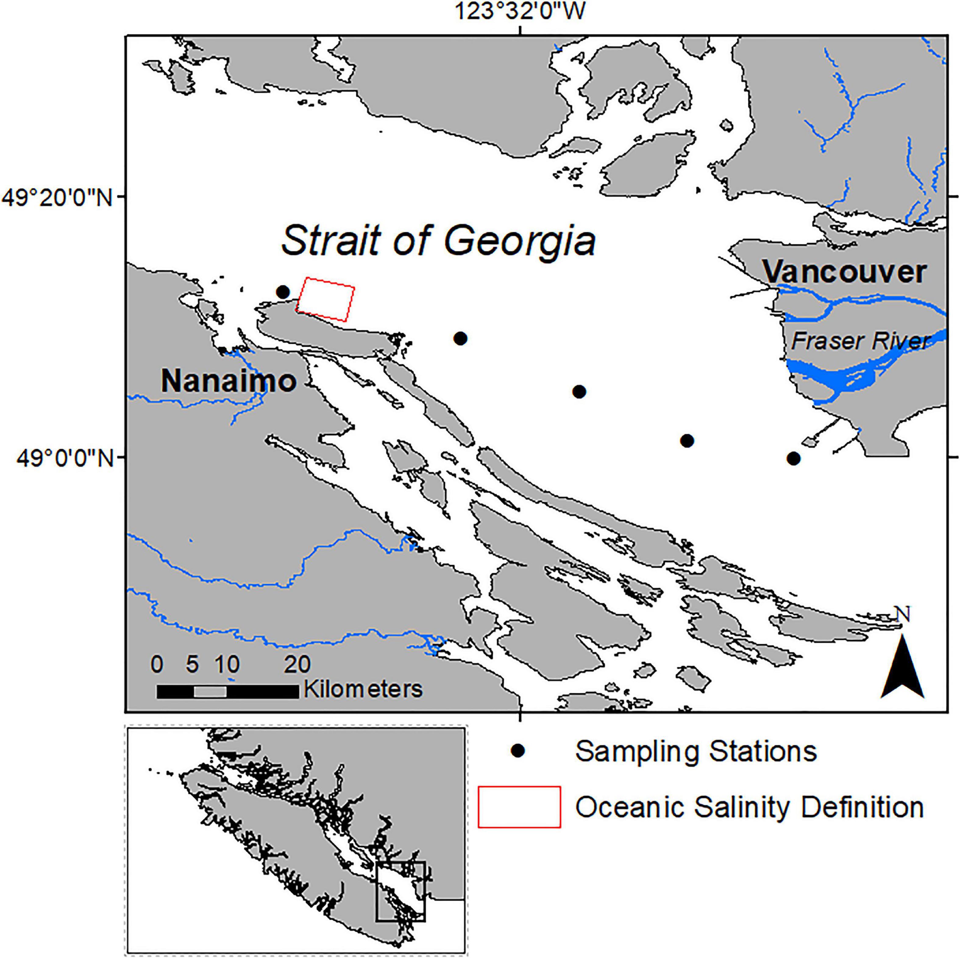
Figure 1. Study area in the Strait of Georgia, British Columbia, Canada. The solid circles indicate the approximate sampling locations of the HPLC measurements along the ferry route between Nanaimo and Vancouver and the solid triangles show the locations of the Duke Point and Tsawwassen ferry terminals in Nanaimo and Vancouver, respectively. The red box indicates the region used to define a salinity threshold to separate oceanic waters and the waters influenced by the Fraser Plume.

Study Area

The data for this study were acquired using a fluorometer equipped flow through system operated by Ocean Networks Canada on board the BC Ferries vessel, Queen of Alberni. The ferry crosses the Strait of Georgia (SoG), a large semi-enclosed sea located on the west coast of Canada between Vancouver Island and mainland British Columbia (Figure 1). This region is characterized by an estuarine circulation largely driven by freshwater input from the Fraser River and saline waters from the Pacific Ocean (Pawloicz et al., 2007). Biogeochemical properties vary across the SoG and are influenced by the dynamics of the Fraser river plume. Waters influenced by the plume are generally highly turbid with a higher concentration of Total Suspended Matter (TSM) and Colored Dissolved Organic Matter (CDOM), whereas waters outside of the plume have relatively higher Chl-a concentration (Johannessen et al., 2006; Loos and Costa, 2010). Given these distinct biogeochemical properties, we define two general water masses in our study area with distinct biogeochemical properties: saline oceanic waters with lower relative turbidity, and less saline plume waters with higher turbidity (hereafter referred to as oceanic and plume waters, respectively).

Discharge from the Fraser River varies over the spring and summer. Peak discharge typically occurs in mid-June following snowpack melt (Masson, 2006). During the spring and summer, increased light availability and wind dynamics also promote conditions favorable to seasonal phytoplankton blooms (Masson and Pena, 2009; Allen and Wolfe, 2013; Phillips and Costa, 2017; Suchy et al., 2019). For example, Masson and Pena (2009) reported average spring and summer Chl-a concentrations were about 4.5 and 1.5 μgL^–1, respectively. However, concentrations over 15.0 mg m^–3 have been observed during spring bloom events (Harrison et al., 1983; Li et al., 2000; Allen and Wolfe, 2013; Phillips and Costa, 2017). As expected, the presence of the river plume in the Strait promotes a high degree of spatial-temporal variation in salinity. Halverson and Pawlowicz (2008) reported annual averages of 26 PSU outside of the plume, and average salinity within the plume ranging from 10 PSU during the spring freshet to 25 PSU during periods of low river flow.

Ferry-Sensor Measurements

Among the different measurements collected by the ferry system, this research used a “FerryBox” system measuring salinity (PSU) acquired by a SeaBird SBE45 thermosalinograph, and Chl-a concentration (ugL^–1) acquired by a WET Labs ECO Triplet fluorometer. Surface solar radiance (Wm^–2) was recorded by a Kipp and Zonen Pyranometer CMP-21100540 located on the upper deck of the ferry, measuring irradiance from 285 to 2800 nm on a plane surface, and navigation data recorded from a dual antenna GPS. Ocean Networks Canada (ONC) installed and maintained all sensors, including the “FerryBox,” located below the main deck, 10 m from the bow, drawing water through the hull along a 1.5 m long pipe. Residence time in the system was ∼30 s and the sampling depth was approximately 2 m (Halverson and Pawlowicz, 2011; Wang et al., 2019). The sensor measurement frequency was 1 Hz, and values were binned into 1-min intervals to align with the timing of concurrent water sampling. The ferry traveled at approximately 20 knots; therefore a 1-min sampling interval yielded a spatial resolution of roughly 620 m.

Fluorometer Characteristics and Biofouling Correction

The WET Labs fluorometer excited Chl-a at 470 nm and detected emitted fluorescence at 695 nm with a Chl-a detection range of 0.015 to 30.0 μgL^–1 (Wet Labs Inc., 2017). Maintenance and cleaning procedures on the Chl-a sensor were carried out by ONC technical staff on a bi-monthly basis during the study period. Protocols developed by ONC for this procedure consist of measuring the fluorescence signal of a standard fluorescent solution (Diet Coke^TM) before and after sensor cleaning. The percent difference between these measurements was used to correct the effects of biofouling across the 2-week period between cleaning dates (Cetinić et al., 2009; Earp et al., 2011; Wang et al., 2019). A daily offset was back-calculated for the interval between each cleaning, assuming a linear change in the effect of biofouling, following the method used for the same system in Wang et al. (2019) (Table 1). To calculate the daily change in fChl-a due to biofouling we divided the percent change in measured fluorescence before and after the sensor was cleaned by the total number of days between sensor cleaning dates. The fChl-a measurements were adjusted based on the number of days since the previous cleaning. For example, the sensor was cleaned on April 26th, 2018 and again on May 10th, 2018, yielding an interval of 14 days. The change in fChl-a between before and after sensor cleaning on May 10 was 5.9%, thus the daily percent change within this cleaning interval was 0.42%. The daily correction increased linearly starting from 0.42% on April 27 and increasing to 5.9% by the end of the cleaning interval. This is considered a first level of correction required for any autonomous Chl-a fluorescence sensor (Cetinić et al., 2009; Roesler, 2014).

TABLE 1

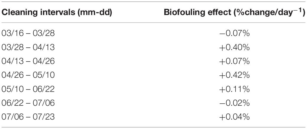
Table 1. Estimated maximum biofouling effect (%change/day) across the study period calculated as the difference in measured fluorescence of a standard solution before and after the WET Labs ECO Triplet fluorometer was cleaned.

Measured surface solar radiation (Wm^–2) was converted into above water PAR (PAR(0)) by multiplying by a factor of 0.47 (Papaioannou et al., 1993). For consistency with the literature, PAR in units of Wm^–2 were converted into photon irradiance in molar units (μE m^–2 s^–1) using a factor of 4.57 (McCree, 1972). Although some variability in this conversion factor is expected, this factor was similar to the range of those observed by Ge et al. (2011) for a similar area and PAR values were in the same range as those observed by Halverson and Pawlowicz (2013) in the SoG.

Extracted Chlorophyll-a Samples

Seawater pumped to the “FerryBox” sensors was split through a manifold with a tapped output for water sampling. This allowed for alignment between sensor measurements and concurrent water sampling. Water samples were drawn from the FerryBox system and extracted Chl-a concentration was derived using HPLC. Samples were collected during 17 transects between March 16, 2018 and August 28, 2018 (n = 62). These discrete samples were aligned with the 1-min average of fChl-a concentration obtained by the WETLabs Chl-a fluorometer based on the time of sampling. Three to five stations were sampled between Duke Point and Tsawwassen (Figure 1) from 13:00 and 14:30 PDT. Triplicate samples taken from the tap were immediately filtered through 0.7 μm Whatman GF/F 25 mm filters, except for 24 samples which were filtered through 47 mm filters due to logistic issues. For these samples, the volume filtered was adapted to allow for Chl-a detection. Filters were immediately frozen on dry ice and stored in dark conditions at −80°C in the lab until pigment extraction (Claustre et al., 2004; Hooker et al., 2010). Pigments were extracted and analyzed by the Baruch Institute of Marine and Coastal Sciences, University of South Carolina using the HPLC method described by Hooker et al. (2010).

Data Processing

Data processing and analysis consisted of several steps to correct data for biofouling (previous section) and systemic sensor bias. We also estimated PAR at 2 m depth to assess the degree of NPQ and evaluate the performance of three NPQ correction methods. Finally, we examined how uncertainty in our calculation of k_z is propagated throughout the entire procedure. These steps are detailed below and outlined in Figure 2.

FIGURE 2

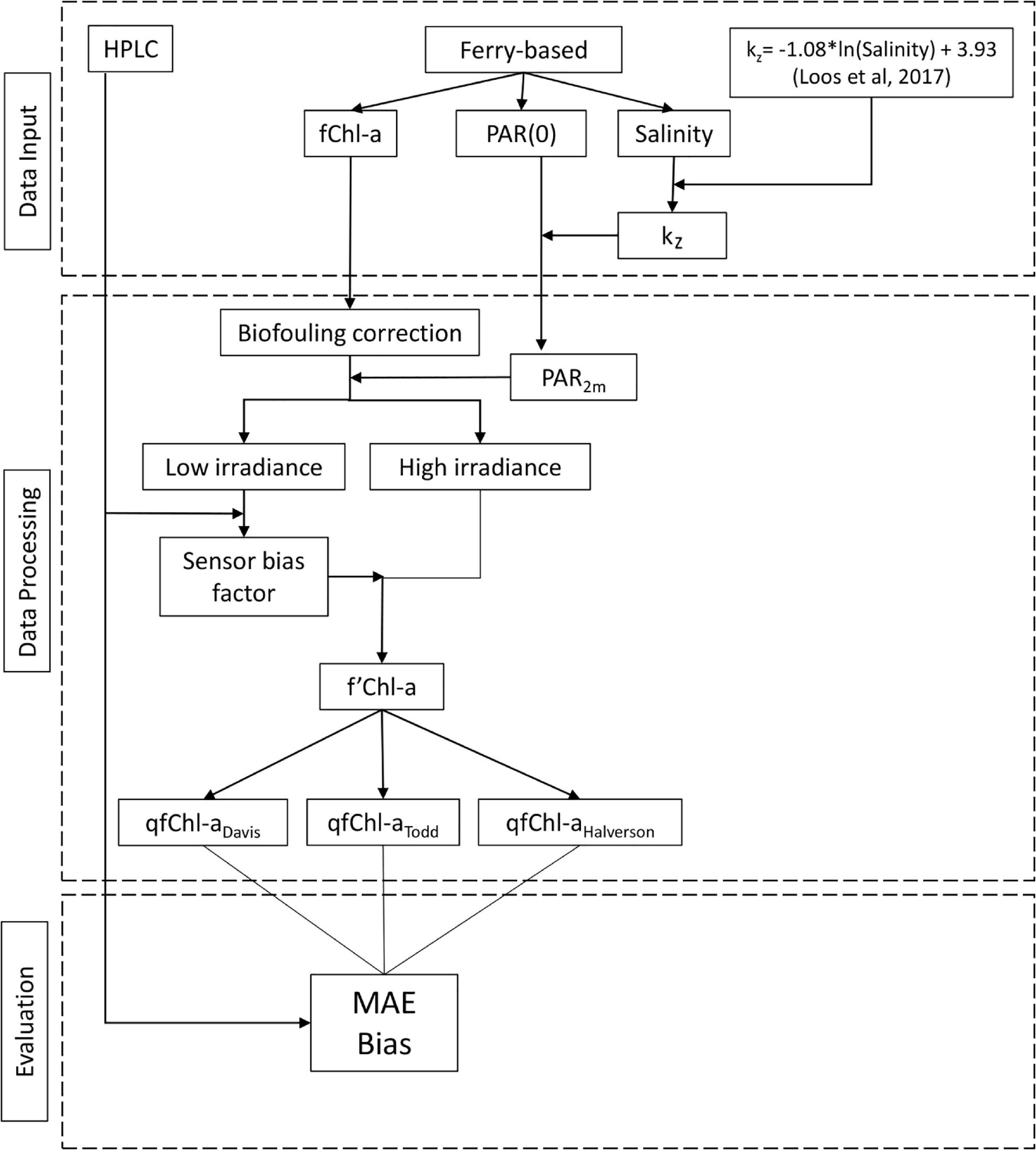
Figure 2. Flowchart showing primary steps in the data analysis, including data inputs, data processing and evaluation.

Defining Underwater PAR

We calculate the PAR_2m extinction coefficient k_z, using a dataset of in situ down-welling irradiance and salinity from the study area (Loos et al., 2017). From this data, we derive a relationship between salinity and k_z, which was then used to estimate k_z based on salinity measurements from the ferry. PAR_2m was calculated according to Kirk (2011):

${\text{PAR}}_{2\text{m}}=\text{PAR}\left(0\right)\exp \left[-\mathrm{PAR}{\mathrm{k}}_{\text{z}}\right](1)$

In this region, light attenuation within the relatively clearer and more saline oceanic waters is primarily driven by phytoplankton, and it is generally lower than in the more turbid less saline plume waters, where attenuation is driven by CDOM and TSM (Johannessen et al., 2006; Loos and Costa, 2010; Loos et al., 2017). As such, a relationship between salinity and k_z was defined using in situ data measured by Loos et al. (2017) in the SoG during the summer, matching oceanographic and irradiance conditions in this study. The authors measured PAR down-welling irradiance and salinity at different depths, allowing the calculation of k_z according to Kirk (2011):

${\text{k}}_{\text{z}}({\text{z}}_1\leftrightarrow {\mathrm{z}}_2)=\frac{1}{{\text{z}}_2-{\text{z}}_1}\ln \left(\frac{{\text{E}}_{\text{d}}({\text{z}}_1)}{{\text{E}}_{\text{d}}\left({\text{z}}_2\right)}\right)(2)$

where E_d(z₁) is the measured PAR down-welling irradiance in μE m^–2 s^–1 at depth z₁ and E_d(z₂) is the PAR down-welling irradiance at depth z₂, approximately 2m. The calculated, k_z values were then regressed against the average salinity within the upper 2m, resulting in the following relationship: k_z = −1.08ln(Salinity) + 3.93 (Figure 3; n = 19, r = −0.72, df = 17, p < 0.01).

FIGURE 3

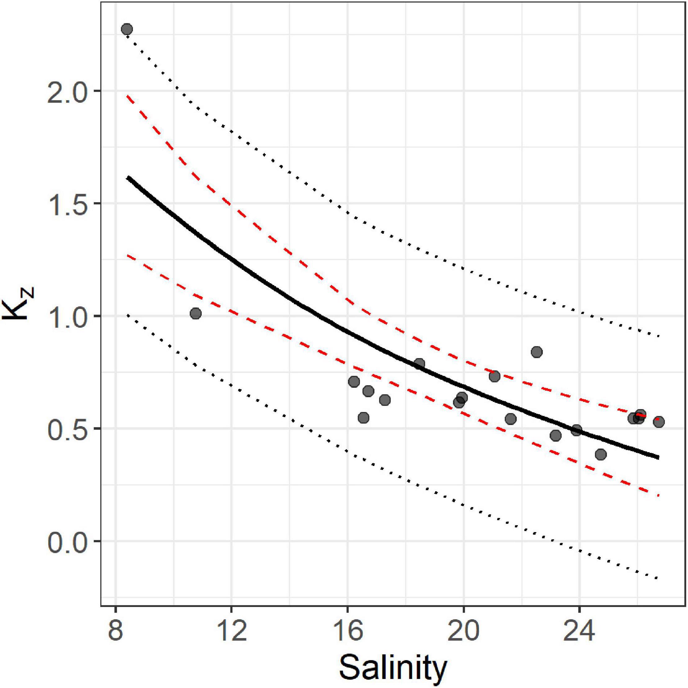
Figure 3. Salinity and modeled kz values based on 19 CTD profiles acquired by Loos et al. (2017). The solid line shows the regression fit, dashed red lines show the 95% confidence interval for the regression, and the dotted black lines show the 95% prediction interval for the data.

Using this equation we estimated k_z for the ferry dataset using salinity measurements acquired by the FerryBox. The mean k_z values for plume and oceanic waters were 1.26 m^–1 (sd = 0.76) and 0.58 m^–1 (sd = 0.13), respectively, similar to the Halverson and Pawlowicz (2013) values of 1.1 and 0.27 m^–1, respectively. Overall, the turbid plume waters have low salinity, higher values of k_z and thus very low irradiance (Figure 4).

FIGURE 4

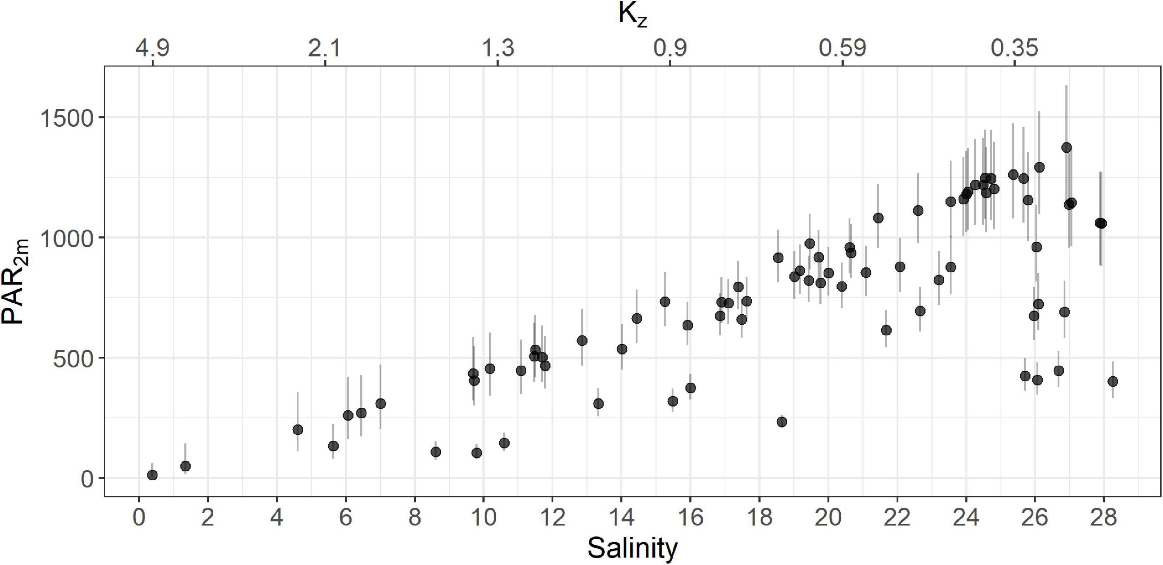
Figure 4. PAR_2m for the entire ferry dataset as a function of salinity (solid circles). Error bars for PAR_2m were calculated using the upper and lower limits of the 95% confidence interval of k_z. The estimated k_z is shown on the secondary x-axis (top). Note that points exhibiting low PAR_2m and low k_z represent samples from cloudy conditions.

Finally, we calculated PAR_2m using Equation 1, resulting in an average of 531 μE m^–2 s^–1 (sd = 277) and 863 μE m^–2 s^–1 (sd = 274) in plume and oceanic waters, respectively. Uncertainty in the estimate of k_z, may impact values of PAR_2m, and consequently the performance of the NPQ correction step. However, as each of the evaluated correction methods use the same PAR_2m input, the relative performance of these methods should be comparable. Uncertainty in the relationship between kz and salinity is greatest when salinity is between 8 and 16 PSU as we only had two samples in this range. To capture this uncertainty, we calculated upper and lower 95% confidence limits for each value of k_z (Figure 3) and used these intervals to calculate corresponding upper and lower limits of PAR_2m (Figure 4).

Correcting Sensor Bias

The second level of data correction addresses systematic bias between fChl-a and HPLC. To correct systemic sensor bias we first subset the ferry dataset into high (n = 56) and low-light (n = 6) samples using a PAR_2m threshold of 200 μE m^–2 s^–1, representing minimal impact of NPQ. This threshold is used by Morrison (2003) and Roesler et al. (2017) and is similar to the threshold for NPQ in the SoG reported by Halverson and Pawlowicz (2013). We used samples acquired in low-light conditions to quantify sensor bias as the ratio between fChl-a and exChl-a. The low-light samples represent conditions in which the effect of NPQ is minimal, thus better isolating the effect of sensor bias. The median ratio of fChl-a and exChl-a for the high-light samples (n = 55) was 0.48 with an Interquartile Range (IQR) of 0.36–0.64, and the median ration for low-light samples (n = 6) was 0.57 with an IQR of 0.41–0.72. The median ration of low-light samples is slightly higher than the ratio for high-light samples. This is consistent with the effect of NPQ, which would be expected to depress fChl-a and decrease the ratio between fChl-a and exChl-a (Kolber et al., 1990; Falkowski and Kolber, 1995). We corrected the fChl-a data (previously corrected for biofouling) by dividing fChl-a by 0.57. Hereafter, we refer to biofouling and sensor corrected as f’Chl-a.

Methods for NPQ Corrections

The third level of correction after biofouling and sensor bias addresses the NPQ effect for f’Chl-a data acquired under high irradiance conditions. The following three methods were considered.

Halverson and Pawlowicz (2013) Model

Halverson and Pawlowicz (2013) corrected fluorescence derived Chl-a concentration obtained by a similar ferry system in the Strait of Georgia for the effect of NPQ using a function originally derived by Cullen and Lewis (1995). The function uses PAR_2m and a threshold value for PAR to estimate unquenched Chl-a concentration. The form of the function is

$\frac{\mathrm{f}{}^{\prime }\mathrm{Chl}\text{-}a}{\text{qfChl-}a}=\text{A}+\left(1-\text{A}\right)\exp \left[\frac{-\left({\text{PAR}}_{2\text{m}}-{\text{PAR}}_{\text{t}}\right)}{\text{C}}\right](3)$

where qfChla is the corrected unquenched Chl-a concentration. PAR_t represents the threshold irradiance for NPQ, defined as the irradiance at which NPQ affects the relationship between fChla and qfChla. Correction for NPQ was applied when PAR_2m exceeded this threshold. The terms A and C are regionally specific constants, defined in Halverson and Pawlowicz (2013). The fitted coefficients for A, C and PAR_t were 0.56 μE m^–2 s^–1, 304 μE m^–2 s^–1, and 182 μE m^–2 s^–1, respectively (Halverson and Pawlowicz, 2013). For this study, Equation-3 was used to correct fChl-a obtained by the ferry system using the coefficients for A,C and PAR_t calculated in Halverson and Pawlowicz (2013) and PAR_2m depth estimated from Equation 1. We hereafter refer to this method as HP2013.

Todd et al. (2009) Model

Todd et al. (2009) used the covariance between PAR_2m and fluorescence to isolate the portion of the fluorescence signal uncorrelated with irradiance. To correct NPQ, the method assumed that f’Chl-a can be modeled as following:

$\mathrm{f}{}^{\prime }\mathrm{Chl}\text{-}a=\text{B}({\text{PAR}}_{2\text{m}})+\text{qfChl-}a(4)$

Where B is an unknown constant, and qfChl-a is the portion of the f’Chl-a signal uncorrelated with surface light, representing the corrected unquenched fluorescence. It can be shown that the term B can be re-written as

$\text{B}=\frac{\text{Cov}(\mathrm{f}{}^{\prime }\mathrm{Chl}\text{-}a,{\mathrm{PAR}}_{2\text{m}})}{\text{Var}({\text{PAR}}_{2\text{m}})}.(5)$

The value for B was −0.0004. Therefore, by re-arranging Equation (4) substituting B from Equation (5), the unquenched fluorescence signal qfChl-a can be calculated as

$\text{qfChl-}a=\text{f}{}^{\prime }\text{Chl-}a+(0.0004){\mathrm{PAR}}_{2\text{m}}(6)$

where fluorescence measurements from the ferry were corrected using Equation-6 and concurrent estimates of PAR_2m. Similar to the Halverson and Pawlowicz (2013) method, no correction for NPQ was performed when PAR_2m was lower than the threshold of 182 μE m^–2 s^–1. We hereafter refer to this method as T2009.

Davis et al. (2008) Model

Davis et al. (2008) uses measured f’Chl-a and PAR_2m to estimate unquenched Chl-a concentration, qfChl-a. The model assumes the relationship between f’Chl-a and qfChl-a is as follows:

$\text{qfChl-}a=\frac{\mathrm{f}{}^{\prime }\mathrm{Chl}\text{-}a}{{\text{q}}_{{\text{PAR}}_{2\text{m}}}}(7)$

where q_PAR2m is the quenching function which depends on PAR_2m. The quenching function q_PAR2m is assumed to have the form

${\text{q}}_{{\text{PAR}}_{2\text{m}}}=\frac{\text{x}}{\text{x}+{\text{PAR}}_{2\text{m}}}(8)$

where x is a constant. Equation (8) has the following properties, when PAR_2m = 0 then q = 1 and subsequently f’Chl-a = qfChl-a. However, as irradiance increases, q_PAR2m approaches 0, and qfChl-a becomes increasingly greater than f’Chl-a. The parameter x was fitted such that the correlation between f’Chl-a and PAR_2m is equal to 0. This optimization isolates the portion of the fluorescence signal that is uncorrelated with irradiance, i.e., unquenched fluorescence. Using the entire dataset we fit a value for x of 5169 that minimized the covariance between qfChl-a and f’Chl-a. By substituting q_PAR2m in Equation 7, the final form of the correction equation is:

$\text{qfChl-}a=\mathrm{f}{}^{\prime }\mathrm{Chl}\text{-}a\left(\frac{\text{x}+{\text{PAR}}_{2\text{m}}}{x}\right)(9)$

Again, no correction for NPQ was performed when PAR_2m was lower than 182 μE m^–2 s^–1. We hereafter refer to this method as D2008.

Evaluation Statistics

NPQ corrected Chl-a concentrations were evaluated against coincident extracted chlorophyll concentration from the HPLC analysis acquired under high irradiance conditions (n = 61). We evaluate method performance using Mean Absolute Error (MAE) representing absolute model accuracy, and Bias representing model overestimation or underestimation. MAE and Bias are defined as follows:

$\text{MAE}=\frac{1}{\text{n}}\sum _{\text{i}=1}^{\text{n}}\left|\text{qfChl}a-\text{exChl}a\right|(10)$

$\text{Bias}=\frac{1}{\text{n}}\sum _{\text{i}=1}^{\text{n}}\text{qfChl}a-\text{exChl}a(11)$

To analyze potential sources of error as a function of different environmental conditions, MAE and Bias were calculated separately for oceanic and plume waters. The optimal NPQ correction was chosen based on the best overall MAE and Bias across both water types. Once the optimal quenching correction was determined we defined a regression equation to calibrate qfChl-a to exChl-a concentrations and analyze the model residuals.

Classifying Plume and Oceanic Waters

Plume and oceanic waters are distinguished based on a variable salinity threshold described in Halverson and Pawlowicz (2011) developed for the SoG. These two classes reflect differences in turbidity (Loos et al., 2017) that may in turn affect the magnitude of NPQ (Halverson and Pawlowicz, 2013). Salinity thresholds (S_threshold) were calculated for each ferry transect, and plume waters were defined where salinity was less than S_threshold and oceanic waters were defined where salinity was greater than S_threshold. To calculate this threshold, we first defined a reference salinity (S_ref) representing waters known to be under the least influence of the plume. For each ferry transect this value was the average of salinity measurements acquired in a fixed area outside of plume waters (Figure 1). For this dataset, the mean value of S_ref was 24.41 and S_threshold was calculated as:

${\text{S}}_{\text{threshold}}=4.8-0.14({\text{S}}_{\text{ref}})(12)$

The values for the constants 4.8 and 0.14 are from Halverson and Pawlowicz (2011) and are specific to this region.

Results

Characterizing Diurnal fChl-a Measurements

Before presenting the results associated with different levels of correction, we characterize diurnal fChl-a patterns and the effect of NPQ in oceanic and plume waters. For this characterization, we sampled fChl-a 1-min averaged measurements from the ferry system across 21 days during the study period (n = 10,610). In total, 11 sunny days (5840 observations) and 10 completely overcast days (4769 observations) were sampled. Each day was subset into three time periods, 5am–8am, 11am–3pm, and 7pm–11pm to capture diurnal changes in fChl-a between the morning, midday and nightime periods, respectively. Average fChl-a were calculated across time-periods, water type and weather conditions (sunny or overcast).

Mean fChl-a concentrations were generally greater in the plume, with concentrations of 1.9 and 1.3 μgL^–1 for plume and oceanic water, respectively. Overall, both water types showed similar diurnal changes in fChl-a concentration, with a general increase in fChl-a over the course of the day (Figure 5). In both plume and the oceanic waters, average fChl-a at night was greater than fChl-a in the morning and at midday. These observations are consistent with the day-time growth cycles of coastal phytoplankton populations reported in other studies (Takahashi et al., 1978; Sosik et al., 2003). We also observed lower midday mean fChl-a on sunny days compared to overcast days in both water types, consistent with the effect of NPQ.

FIGURE 5

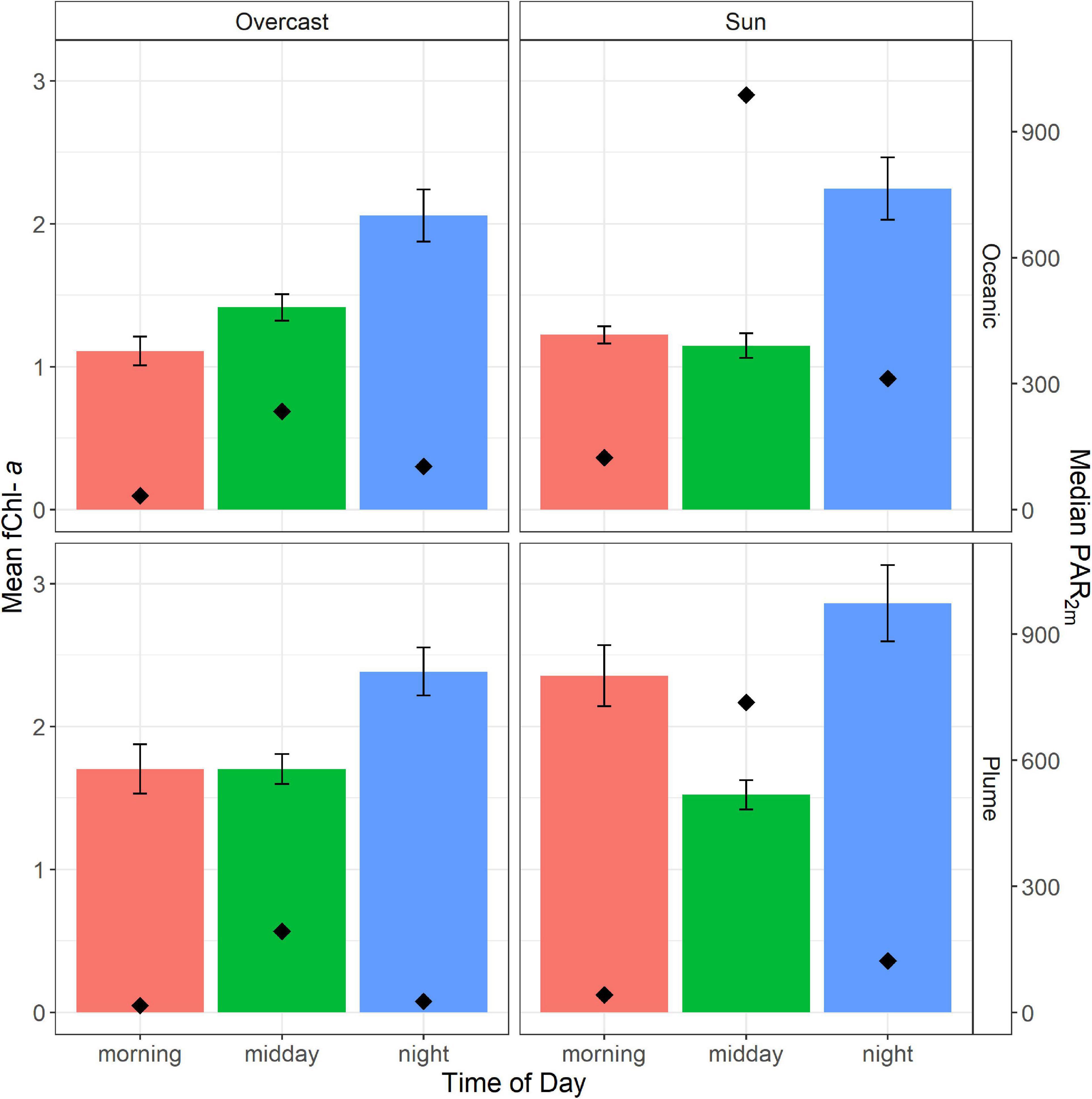
Figure 5. Average chlorophyll-a concentration obtained by the FerryBox across three time periods and in sunny and overcast conditions. Error bars represent 95% confidence intervals for mean Chl-a concentration. The top row shows average conditions in oceanic water (n = 4927) and the bottom row shows average conditions in the plume (n = 5679). Median PAR^2m is shown on the secondary y-axis and is represented by black diamonds.

Assessment of Different Levels of Correction and Methods

All subsequent analysis is conducted using 61 samples of exChl-a concentration from HPLC analysis matched to 1-min average fChl-a sampled at midday when PAR_2m is greatest and fChl-a is lowest likely due NPQ (Figure 5). Within a 1-min interval, the fluorometer records 56 measurements. These were typically homogenous as the average coefficient of variation was < 5%. Three samples had a coefficient of variation greater than 20%, likely due to rapid changes in fChl-a concentration as the ferry crossed the Fraser River plume front. In these cases, the 1-min median of fChl-a concentration was used instead of the average. The range of 1-min averaged fChl-a was 0.37 to 9.15 μg L^–1, with an overall mean of 1.68 μg L^–1 (n = 62). In plume waters mean fChl-a was 1.53 μg L^–1 (n = 32), and in oceanic waters mean fChl-a was 1.84 μg L^–1 (n = 29). The maximum effect of biofouling was a daily 0.42% increase in fChl-a over a period of 14 days (Table 1). After correcting for biofouling and sensor bias, global average f’Chl-a was 2.93 μg L^–1, with average values of 2.68 and 3.21 μg L^–1 in plume and oceanic waters, respectively. By comparison global average exChl-a concentration was 3.82 μg L^–1, with average values for plume and oceanic samples were 3.57 and 4.11 μg L^–1, respectively.

We assess the accuracy of the biofouling, sensor bias, and NPQ correction steps, using Bias to represent over and under-estimation of exChl-a and MAE to represent the absolute deviation from exChl-a (Table 2). A detailed assessment of each approach considering different levels of correction and water classes is presented in Table 2. The basic level of correction, with only biofouling, exhibited as expected the poorest performance, with the highest MAE (2.22) and Bias (−2.14) independent of water type. MAE and Bias were also greater in oceanic waters compared to plume waters (Table 2). The second level of correction including sensor bias (f’Chl-a) substantially improved overall MAE (1.37) and Bias (−0.89), however concentrations were still underestimated in both plume and oceanic waters (Table 2).

TABLE 2

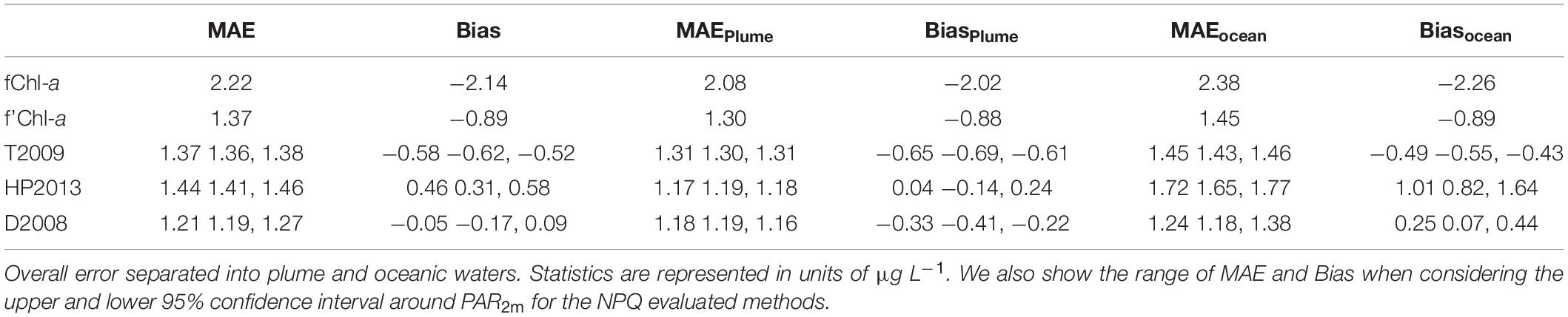
Table 2. Comparison of error statistics for each step of the correction procedure: (1) biofouling correction (fChl-a), (2) adjusted for sensor bias (f’Chl-a), and (3) the three NPQ correction methods.

The following NPQ corrections resulted in a general improvement in error statistics, especially in Bias. To account for the uncertainty in k_z, we calculated error statistics using the high and low PAR_2m estimates derived from the upper and lower 95% confidence limits on k_z. As none of the intervals in MAE and Bias overlap (Table 2) between the three NPQ corrections, we conclude that the methods are statistically distinct (i.e., not interchangeable). Overall, the T2009 method underestimated Chl-a concentrations in both water types, with Bias of −0.65 and −0.49 in plume and oceanic waters, respectively. Furthermore, overall MAE (1.37) did not improve compared to overall MAE for f’Chl-a. In terms of Bias, the HP2013 method was the best in low-light plume conditions (0.04), but was the worst in high irradiance oceanic waters (1.01). Overall MAE (1.44) for HP2013 was was also greater than MAE for f’Chl-a (1.37). Comparatively, the D2008 method showed the best overall Bias (−0.05) which was a result of underestimation in plume waters (−0.33) and overestimation in oceanic waters (0.25) by a similar margin. Overall MAE was also the lowest across all levels of correction. For these reasons, we consider the D2008 method to be the “optimal” NPQ correction. A more robust residual error analysis was conducted on this dataset, where qfChl-a_Davis hereafter refers to chlorophyll-a concentration corrected for biofouling, sensor bias and NPQ using the D2008 method.

We calculated a linear regression between the qfChl-a_Davis and exChl-a and assessed patterns in standardized residuals of this model. Data were log transformed to account for the non-normal distribution of Chl-a (Seegers et al., 2018). The resulting regression equation was:

log₁₀ (exChl-a) = −0.06 + 1.01^∗ log₁₀ (qfChl-a_Davis), with r = 0.81 (Figure 6). No obvious patterns were apparent in the standardized residuals as a function of qfChl-a_Davis, salinity, CDOM concentration and PAR_2m (Figure 6). However, positive residuals are generally associated with higher qfChl-a_Davis, suggesting that this correction tends to underestimate exChl-a at higher concentrations (Figure 6). The regression between log₁₀(exChl-a) and f’Chl-a corrected with the HP2013 and T2009 methods appear similar to the D2008 method and are shown in Figure 7.

FIGURE 6

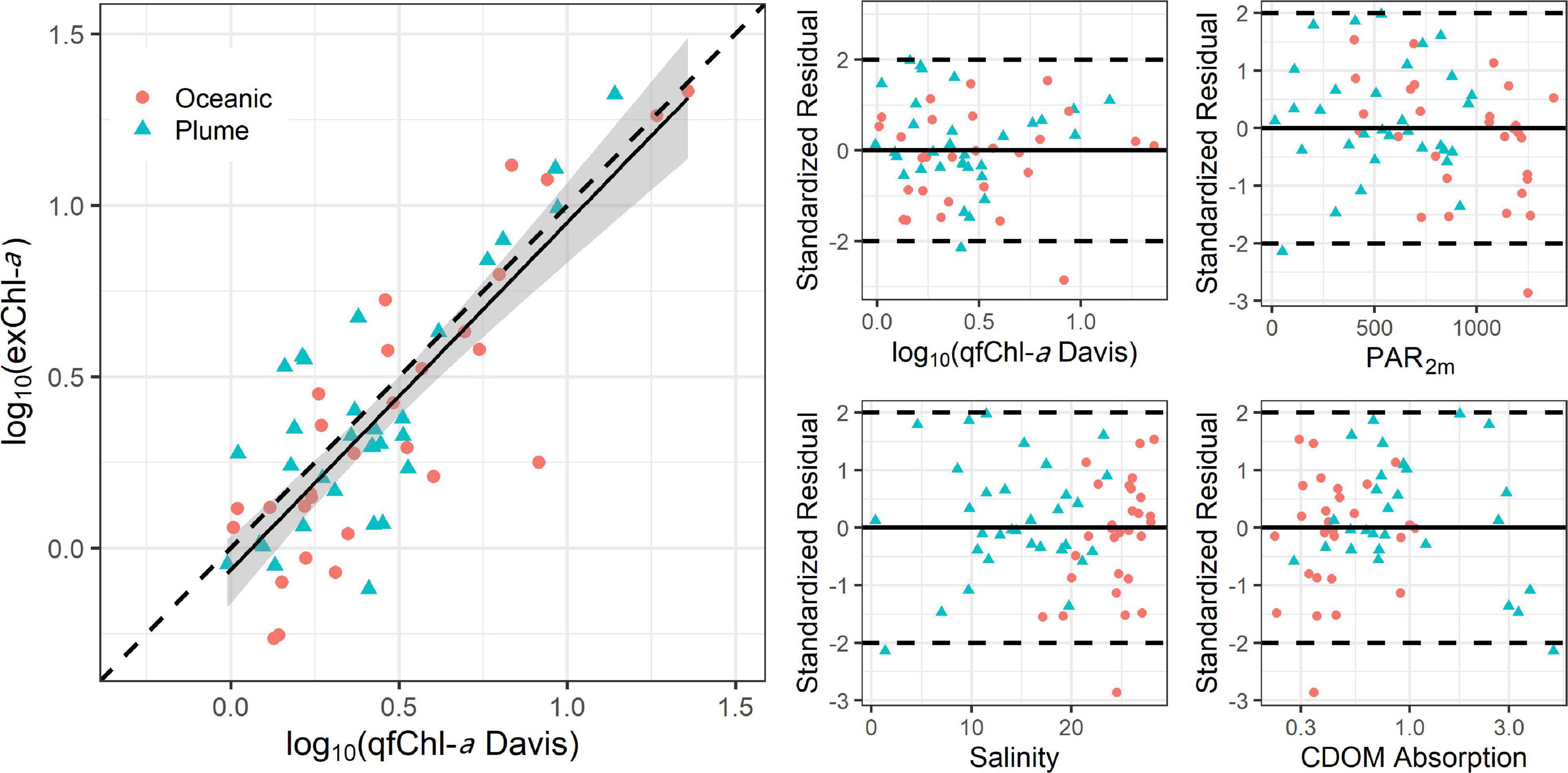
Figure 6. Regression between log10 transformed qfChl-a_Davis and HPLC (left) and standardized residual plots as a function of qfChl-a_Davis, PAR_2m, CDOM absorption and salinity (right). The red circles are sampled from the plume and the blue triangles are sampled in oceanic waters. Note that data were log₁₀ transformed to account for the non-normal distribution of Chl-a (Seegers et al., 2018).

FIGURE 7

Figure 7. Regression between log10 transformed qfChl-a_Todd and HPLC (left) and qfChl-a_Halverson (right). The red circles are sampled from the plume and the blue triangles are sampled in oceanic waters. Note that data were log₁₀ transformed to account for the non-normal distribution of Chl-a (Seegers et al., 2018).

Discussion

Instrumented ferries have the potential to provide continuous measurements of surface Chl-a concentration at high spatial and temporal resolution and at relatively low cost compared to other autonomous platforms (Petersen, 2014). However, care should be taken because surface in vivo Chl-a fluorescence measurements may be impacted by many interacting factors, including sensor biofouling and bias (Roesler, 2014; Roesler et al., 2017), NPQ (Serra et al., 2009), and CDOM contamination (Proctor and Roesler, 2010; Xing et al., 2017). Here, we propose a method to improve estimates of Chl-a concentration acquired from an instrumented ferry. We quantify the impact of these sources of error and evaluate three potential NPQ correction methods proposed in the literature. In particular, we highlight the importance of assessing error in the measured Chl-a signal across oceanic and freshwater influenced waters.

We addressed two sources of error at the sensor level: biofouling and systemic bias. Fluorometer biofouling can be broadly categorized into biofilm and frondular biofouling (Roesler, 2014). Biofilm can accumulate on the optical windows of the sensor resulting in an increased fluorescence signal while frondular biofouling results from the growth of larger organisms on the sensor that can have a variable effect on the fluorescence signal (Roesler, 2014). Our data showed slight sensor drift over time with an average increase of 0.13% per day, typical of other fluorescence sensors (Delauney et al., 2009). This drift resulted in relatively little impact on fChl-a measurements, with a maximum increase of 6.4% within the approximately 2 weeks intervals between cleaning (Table 1). For our oceanographic conditions, 2 weeks cleaning intervals are crucial to retrieve high quality data and avoid degradation due to biofouling. Delauney et al. (2009) have shown that the effects of biofouling induced sensor drift starting 13 days after deployment, reaching values about 10 times higher after 2 months. These results will vary depending on the oceanographic conditions of the sampled area (Roesler, 2014; Zeng and Li, 2015).

With respect to potential sensor bias, Roesler et al. (2017) used a global dataset of in vivo fluorescence measurements and identified a global overestimation factor of 2 for commonly used WET Labs fluorometers, the same manufacture of the sensor used in this research. The authors associate this systemic bias to a combination of factors including, differences between the experimental conditions of factory calibrations and variability of phytoplankton species, cell size, growth state, and pigment composition in natural populations. Using a small number of samples under low-irradiance, we found sensor underestimation by a factor of 0.57. The discrepancy between our factor and the global bias observed by Roesler et al. (2017) may be due to differences in water type, as the authors primarily sampled open ocean regions. Our slope factor is most similar to the factor of 0.67 recorded in the inland Black Sea by the same authors. By using this ratio to correct our dataset, we accounted for a substantial portion of the difference between fChl-a and exChl-a. However, to increase confidence in this correction we recommend collecting more low-irradiance samples across different water types for a broader representation considering the fluorescence signal to sensor bias ratio.

Biofouling and sensor bias should first be addressed for all Chl-a fluorescence data as a baseline correction. However, as has been extensively reported in the literature (Kiefer, 1973; Falkowski and Kolber, 1995; Serra et al., 2009; Xing et al., 2012), and further demonstrated with our dataset (Figure 2), in vivo Chl-a fluorescence measurements can be impacted by NPQ at high irradiance. Our data showed that correcting for NPQ further improved estimates of Chl-a concentration beyond the initial biofouling and sensor bias steps. The three corrections that we applied varied in performance and underlying methodology. The HP2013 correction differed the most in the underlying method. This method relied on regionally specific coefficients and an empirical function, while the T2009 and D2008 methods use the covariance between measured fChl-a and irradiance, and therefore are not regionally specific. This study used the same fitted constants as calculated in Halverson and Pawlowicz (2013) given that both works represent similar waters and used data from an instrumented ferry operating in the Strait of Georgia. However, Halverson and Pawlowicz (2013) defined the fitted constants using the relationship between CTD Chl-a fluorescence and extracted chlorophyll-a derived from spectrofluorometric analysis, while we use HPLC as our validation source. As fluorometric and HPLC measurements generally provide slightly different Chl-a concentrations (Mueller et al., 2003), the performance of HP2013 may improve by matching the techniques used to fit the coefficients and validate the correction.

The D2008 and T2009 methods as presented in this paper are broadly applicable to other data sets due to the lack of region-specific constants. While we applied the D2008 and T2009 methods to data spanning March to August, 2018 over longer time series it may be preferable to aggregate data seasonally and perform separate corrections on each dataset. Davis et al. (2008) used Spray underwater gliders to measure physical and biological properties and computed separate NPQ corrections for each glider deployment, while Todd et al. (2009) used similar glider systems and binned into data groups of 32 dives. The primary assumption of these methods is that the covariance between fChl-a and irradiance is negative. This may be a problem in small or noisy datasets, or where fChl-a and PAR do not vary much.

For any of the evaluated methods, uncertainty in the estimate of k_z impacts PAR_2m and the magnitude of NPQ. While we used an independent dataset of salinity and PAR profiles to derive k_z, if profiling data is unavailable, empirical models have been proposed to estimate the diffuse attenuation coefficient using satellite derived ocean color for open ocean and coastal environments (Wang et al., 2009). Beyond uncertainties in light availability, other sources of error associated with in vivo Chl-a fluorescence include the effect of other fluorescing matter such as Colored Dissolved Organic Material (Proctor and Roesler, 2010; Röttgers and Koch, 2012). The WET Labs ECO Triplet fluorometer installed on the ferry simultaneously records Chl-a and CDOM fluorescence in separate channels, with the Chl-a channel exciting samples at 470 nm and recording emissions at 695 nm and the CDOM channel exciting at 370 nm and recording emissions at 460 nm (WET Labs Inc., 2017). However, high CDOM concentration may impact the fluorescence signal recorded in the Chl-a channel by absorbing the fluorometer excitation energy, absorbing Chl-a emission energy or contributing to the fluorescence recorded in the Chl-a channel (Proctor and Roesler, 2010). For example, Proctor and Roesler (2010) observed a strong linear relationship between recorded Chl-a fluorescence and CDOM concentration, and Xing et al. (2017) suggested that up to 4% of CDOM fluorescence in oceanic waters may contribute to fluorescence recorded in the Chl-a channel.

Within the SoG, CDOM concentration tends to be relatively high, especially within the turbid plume waters (Loos and Costa, 2010). However, as illustrated in Figure 6 regression residuals do not show any apparent pattern in association with CDOM concentration, suggesting that potential error due to CDOM contamination is likely consistent across the dynamic range of observed CDOM. We did not explicitly correct for CDOM contamination in this procedure because our data did not allow us to separate errors due to sensor bias and CDOM contamination. The low irradiance samples used to correct sensor bias generally came from highly turbid plume waters, where we would also expect to see the greatest CDOM contamination. Thus, potential CDOM contamination in these samples may have resulted in overestimation of sensor bias in water with relatively low CDOM concentration. Thus, additional work measuring fluorometer response to controlled dilutions of CDOM is likely needed to separate sensor bias and CDOM contamination effects (Proctor and Roesler, 2010).

As previously mentioned, different phytoplankton groups also impact the systematic bias between in vivo fluorescence and chlorophyll-a concentrations (Proctor and Roesler, 2010). In the SoG, phytoplankton abundance is greatest in the spring and summer and typically very low through the winter months (Masson and Pena, 2009; Suchy et al., 2019). Concurrent HPLC analysis showed that diatoms dominate from March to June 2018 and small flagellates become dominate toward the end of the summer (Suseelan et al., 2021). This seasonal transition of phytoplankton groups is typical for the Strait of Georgia (Harrison et al., 1983; Taylor and Haigh, 1993). Although it is challenging to untangle the impact of different environmental and biological factors on the fluorescence yield in natural samples (Suggett et al., 2009), it is known that phytoplankton groups and community size influence on those physiological responses, depending on the light history and nutritional stress (Giannini and Ciotti, 2016; Schuback and Tortell, 2019). Therefore, the shift in phytoplankton taxonomical groups reported in the SoG is expected to add a seasonal effect on the relationship between fluorescence signal and chlorophyll-a concentration, as this relationship has been shown to vary among species of diatoms, dinoflagellates and cyanobacteria in monospecific cultures (Proctor and Roesler, 2010). Future work should consider the effects of variable phytoplankton community composition during long-term monitoring studies.

Our results highlight the importance of correcting and validating in vivo fluorescence-based measurements of Chl-a obtained by instrumented ferries, as there may be substantial differences between in vivo fluorescence and extracted concentration. By correcting for potential biofouling effects, sensor bias and performing a correction for NPQ, we can obtain measurements of Chl-a concentration based on in vivo fluorescence from ships of opportunity with a greater degree of confidence. This source of autonomous, continuous data acquisition is an important tool in monitoring phytoplankton dynamics in coastal waters and can be used to complement satellite retrieved observations. In coastal regions such as the Strait of Georgia, where cloud cover prevents continuous satellite-based retrieval of Chl-a concentrations (Carswell et al., 2017; Hillborn and Costa, 2018; Suchy et al., 2019), ferry based estimates could be combined with satellite data to fill data gaps (Lavigne et al., 2012). As such, correcting ferry based fChl-a estimates for NPQ is an important step in merging these two data sources.

Conclusion

We outline a systematic approach to correct ferry based estimates of Chl-a for the effect of biofouling, sensor bias and NPQ. Briefly, the method is as follows:

(1) Apply a daily correction for sensor biofouling using the difference between measured fluorescence of a standard solution before and after sensor cleaning, assuming a linear increase or decrease in biofouling between cleaning dates.

(2) Calculate PAR at the depth of ferry sampling using an estimated attenuation coefficient k_z. In this analysis a regression equation between salinity and k_z was used to calculate k_z for the entire ferry dataset.

(3) Correct potential sensor bias by comparing HPLC to fluorescence based estimates of Chl-a acquired in low-irradiance conditions (assuming minimal to no effect of NPQ).

(4) Correct NPQ using concurrent estimates of PAR_2m with the D2008 method, which removes the portion of the fChl-a signal that is correlated with PAR_2m.

Estimates of Chl-a concentration obtained by instrumented ferries are often impacted by environmental and sensor specific factors that introduce uncertainty in the relationship between measured in vivo fluorescence and Chl-a concentration. If these inaccuracies can be resolved, ships of opportunity can be used to increase the spatial and temporal resolution of data at low cost, and to validate and complement other sources of Chl-a concentration such as satellite retrievals. To accomplish this, we demonstrate that the method proposed by Davis et al. (2008) can be used to correct near-surface fluorescence based Chl-a concentration in our region or similar water types. As one of several ferry monitoring programs operating in complex coastal waters (e.g., Codiga et al., 2012; Petersen, 2014), our work reinforces the importance of accurate validation measurements and error quantification in highly dynamic waters.

Data Availability Statement

The raw data supporting the conclusions of this article will be made available by the authors, without undue reservation.

Author Contributions

HT-S performed data analysis and wrote the manuscript. FG provided edits to the manuscript and assisted with data analysis. ARS contributed expertise on the ferrybox system and provided edits for the manuscript. MC was the primary investigator and provided edits on the manuscript. All authors contributed to the article and approved the submitted version.

Conflict of Interest

The authors declare that the research was conducted in the absence of any commercial or financial relationships that could be construed as a potential conflict of interest.

Publisher’s Note

All claims expressed in this article are solely those of the authors and do not necessarily represent those of their affiliated organizations, or those of the publisher, the editors and the reviewers. Any product that may be evaluated in this article, or claim that may be made by its manufacturer, is not guaranteed or endorsed by the publisher.

Funding

This work was made possible with support from NSERC NCE MEOPAR – Marine Environmental Observation, Prediction and Response Network, the Canadian Space Agency (FAST 18FAVICB09), the Pacific Salmon Foundation, the Canadian Foundation for Innovations (CFI), an NSERC Undergraduate Student Research Award (USRA) to HT-S, and an NSERC Discovery Grant to MC. This is publication number 61 from the Salish Sea Marine Survival Project (marinesurvivalproject.com).

Acknowledgments

The ferry data used in this work were provided by Ocean Networks Canada, with calibrations supported by the Marine Environmental Observation Prediction and Response Network (MEOPAR) Observation Core. The ferry-based data are available online (http://www.oceannetworks.ca/data-tools). We would also like to thank ONC staff Ian Beliveau, Will Glatt, and Keely Lulliwitz.

References

Allen, S. E., and Wolfe, M. A. (2013). Hindcast of the timing of the spring phytoplankton bloom in the strait of georgia, 1968-2010. Prog. Oceanogr. 115, 6–13. doi: 10.1016/j.pocean.2013.05.026

CrossRef Full Text | Google Scholar

Anderson, J. H., Harvey, T., Kallenbac, E. M. F., Murray, C., Hjermann, D., Kristiansen, T., et al. (2017). Statistical Analyses of Chlorophyll-a Data Sampled by a Ferrybox on the Oslo-Kiel Ferry and by the NOVANA Programme. Copenhagen: NIVA Denmark Water Research.

Google Scholar

Anderson, S. R., Diou-Cass, Q. P., and Harvey, E. L. (2018). Short-term estimates of phytoplankton growth and mortality in a tidal estuary. Limnol. Oceanogr. 63, 2411–2422. doi: 10.1002/lno.10948

CrossRef Full Text | Google Scholar

Balch, W. M., Drapeau, D. T., Bowler, B. C., Booth, E. S., Goes, J. J., Ashe, A., et al. (2004). A multi-year record of hydrographic and bio-optical properties in the Gulf of maine: I. spatial and temporal variability. Prog. Oceanog. 63, 57–98. doi: 10.1016/j.pocean.2004.09.003

CrossRef Full Text | Google Scholar

Behrenfeld, M. J., Westberry, T., Boss, E., O’Malley, R. T., Siegel, D. A., Wiggert, J. D., et al. (2009). Satellite-Detected fluorescence reveals global physiology of ocean phytoplankton. Biogeosciences 6, 779–794.

Google Scholar

Biermann, L., Guinet, C., Bester, M., Brierley, A., and Boehme, L. (2015). An alternative method for correcting fluorescence quenching. Ocean Sci. 11, 83–89. doi: 10.5194/os-11-83-2015

CrossRef Full Text | Google Scholar

Carswell, T., Costa, M., Young, E., Komick, N., Gower, J., and Sweeting, R. (2017). Evaluation of MODIS-Aqua atmospheric correction and chlorophyll products of western north american coastal waters based on 13 years of data. 2017. Remote Sens. 9:1063. doi: 10.3390/rs9101063

CrossRef Full Text | Google Scholar

Cetinić, I., Toro-Farmer, G., Ragan, M., Oberg, C., and Jones, B. H. (2009). Calibration procedure for Slocum glider deployed optical instruments. Opt. Express. 17, 420–430.

Google Scholar

Claustre, H., Hooker, S. B., Van Heukele, L., Berthon, J., Barlow, R., Ras, J., et al. (2004). An intercomparison of HPLC phytoplankton pigment methods using in vivo samples: application to remote sensing and database activities. Mar. Chem. 85, 41–61. doi: 10.1016/j.marchem.2003.09.002

CrossRef Full Text | Google Scholar

Cloern, J. E., and Jassby, A. D. (2008). Complex seasonal patterns of primary producers at the land-sea interface. Ecol. Lett. 11, 1294–1303. doi: 10.1111/j.1461-0248.2008.01244.x

PubMed Abstract | CrossRef Full Text | Google Scholar

Codiga, D. L., Balch, W. M., Gallager, S. M., Holthus, P. M., Paerl, H. W., Sharp, J. H., et al. (2012). Ferry-based Sampling for Cost-Effective, Long-Term, Repeat Transect Multidiciplinary Observation Products in Coastal and Estuarine Ecosystems. Summit, VA: Community While Paper, IOOS.

Google Scholar

Cullen, J. J. (1982). The deep Chlorohpyll maximum: comparing vertical profiles of chlorophylla. Can. J. Fish. Aquat. Sci. 29, 791–803. doi: 10.1139/f82-108

PubMed Abstract | CrossRef Full Text | Google Scholar

Cullen, J. J., and Lewis, M. R. (1995). Biological processes and optical measurements near the sea surface: some issues relevant to remote sensing. J. Geophys. Res. 100, 767–784.

Google Scholar

Davis, R. E., Ohman, M. D., Rudnick, D. L., and Sherman, J. T. (2008). Glider surveillance of physics and biology on the Southern California current system. Limnol. Oceanogr. 53, 2151–2168. doi: 10.4319/lo.2008.53.5_part_2.2151

CrossRef Full Text | Google Scholar

Delauney, L., Compere, C., and Lehaitre, M. (2009). “Biofouling protection for marine underwater observatories sensors,” in proceedings of the EUROPE Oceans 09, (Bremen).

Google Scholar

Earp, A., Hanson, C. E., Raplh, P. J., Brando, V. E., Allen, S., Baird, M., et al. (2011). Review of fluorescent standards for calibration of in vivo fluorometers: reccomendations applied in coastal and ocean observing Platforms. Opt. Express 19, 26768–26782. doi: 10.1364/oe.19.026768

PubMed Abstract | CrossRef Full Text | Google Scholar

Falkowski, P. G., Barber, R. T., and Smetacek, V. (1998). Biogeochemical controls and feedbacks on ocean primary production. Science 281, 200–206. doi: 10.1126/science.281.5374.200

PubMed Abstract | CrossRef Full Text | Google Scholar

Falkowski, P. G., and Kolber, Z. (1995). Variations in chlorophyll fluorescence yields in phytoplankton in the world oceans. Funct. Plant Biol. 22, 341–355. doi: 10.1071/pp9950341

CrossRef Full Text | Google Scholar

Ge, S., Smith, R. G., Jacovides, C. P., Kramer, M. G., and Carruthers, R. I. (2011). Dynamics of photosynthetic photon flux density (PPFD) and estimates in coastal northern California. Theor. Appl. Climatol. 105, 107–118. doi: 10.1007/s00704-010-0368-6

CrossRef Full Text | Google Scholar

Giannini, M. F. C., and Ciotti, A. M. (2016). Parameterization of natural phytoplankton photo-675 physiology: effects of cell size and nutrient concentration. Limnol. Oceanogr. 61, 1495–1676. doi: 10.1002/lno.10317

CrossRef Full Text | Google Scholar

Halverson, M. J., and Pawlowicz, R. (2008). Estuarine forcing of a river plume by river flow and tides. J. Geophys. Res. 113:C09033.

Google Scholar

Halverson, M. J., and Pawlowicz, R. (2011). Entrainment and flushing time in the Fraser River estuary and plume from a steady salt balance analysis. J. Geophys. Res. 116:C08023.

Google Scholar

Halverson, M. J., and Pawlowicz, R. (2013). High resolution observations of chlorophyll-a biomass from an instrumented ferry: influence of the Fraser River plume from 2003-2006. Cont. Shelf Res. 59, 52–64. doi: 10.1016/j.csr.2013.04.010

CrossRef Full Text | Google Scholar

Harashima, A., and Kunugi, M. (2000). CGER-Report, National Institude for Environmental Studies, Environmental Agency of Japan. Tokyo: Environmental Agency of Japan. CGER-M007-2000.

Google Scholar

Harrison, P. J., Fulton, J. D., Taylor, F. J. R., and Parsons, T. R. (1983). Review of the biological oceanography of the Strait of Georgia: pelagic environment. Can. J. Fish. Aquat. Sci. 40, 1064–1094. doi: 10.1139/f83-129

PubMed Abstract | CrossRef Full Text | Google Scholar

Hillborn, A., and Costa, M. (2018). Applications of DINEOF to satellite-derived chlorophyll-a from a productive coastal region. Remote Sens. 10:1449. doi: 10.3390/rs10091449

CrossRef Full Text | Google Scholar

Holley, S. E., Purdie, D. A., Hydes, D. J., and Hartman, M. C. (2007). 5 Years of Plankton Monitoring in Southampton Water and the Solent Including FerryBox, Dock Monitor and Discrete Sample Data. Southampton: National Oceanography Centre, Southampton. Report no: 31 [unpublished manuscript].

Google Scholar

Hooker, S. B., Claustre, H., and Ras, J. (2010). “The first SeaWiFS HPLC analysis round-robin experiment (SeaHARRE-1), NASA Tech,” in Memo. 2000-206982, eds S. B. Hooker and E. R. Firestone (Greenbelt, MA: NASA Goddard Space Flight Center),

Google Scholar

Jackson, J. M., Thomson, R. E., Brown, L. N., Willis, P. G., and Borstad, G. A. (2015). Satellite chlorophyll off the British Columbia Coast, 1997-2010. 2015. J. Geophys. Res. Oceans 120, 4709–4728. doi: 10.1002/2014JC010496

CrossRef Full Text | Google Scholar

Johannessen, S. C., Masson, D. L., and Macdonald, R. W. (2006). Distribution and cycling of suspended particles inferred from transmissivity in the strait of georgia, haro strait and juan de fuca strait. Atmos-Ocean 44, 17–27. doi: 10.3137/ao.440102

CrossRef Full Text | Google Scholar

Kiefer, D. A. (1973). Fluorescence properties of natural phytoplankton populations. Mar. Biol. 22, 263–269. doi: 10.1007/bf00389180

CrossRef Full Text | Google Scholar

Kirk, J. T. O. (2011). Light and Photosynthesis in Aquatic Ecosystems, 3rd Edn. Cambridge: Cambridge University Press.

Google Scholar

Kolber, Z., Wyman, K. D., and Falkowski, P. G. (1990). Natural variability in photosynthetic energy conversion efficiency: a field study in the Guld of Maine. Limnol. Oceanogr. 35, 72–79. doi: 10.4319/lo.1990.35.1.0072

CrossRef Full Text | Google Scholar

Lavigne, H., D’Ortenzio, F. D., Claustre, H., and Poteau, A. (2012). Towards a merged satellite and in situ fluorescence ocean chlorophyll product. Biogeosciences 9, 2111–2125. doi: 10.5194/bg-9-2111-2012

CrossRef Full Text | Google Scholar

Li, M., Gargett, A., and Denman, K. (2000). What determines seasonal and interannual variability of phytoplankton and zooplankton in strongly estuarine systems? application to the semi-enclosed estuary of Strait of Georgia and Juan de Fuca Strait. Estuarine Coastal Shelf Sci. 50, 467–488. doi: 10.1006/ecss.2000.0593

CrossRef Full Text | Google Scholar

Loos, E. A., and Costa, M. (2010). Inherent optical properties and optical mass classification of the waters of the Strait of Georgia, British Columbia, Canada. Prog. Oceanogr. 87, 114–156. doi: 10.1016/j.pocean.2010.09.004

CrossRef Full Text | Google Scholar

Loos, E. A., Costa, M., and Johannessen, J. (2017). Underwater optical environment in the coastal waters of British Columbia, Canada. FACETS 2, 872–891. doi: 10.1139/facets-2017-2074

PubMed Abstract | CrossRef Full Text | Google Scholar

Lorenzen, C. J. (1966). A method for the continuous measurement of in vivo chlorophyll concentration. Deep-Sea Res. 13, 223–227. doi: 10.1016/0011-7471(66)91102-8

CrossRef Full Text | Google Scholar

Lorenzen, C. J. (1967). Determination of chlorophyll and pheo-pigments: spectrophotometric equation. Limnol. Oceanogr. 12, 343–346. doi: 10.4319/lo.1967.12.2.0343

CrossRef Full Text | Google Scholar

MacIntyre, H. L., Lawrenz, E., and Richardson, T. L. (2010). “Taxonomic discrimination of phytoplankton by spectral fluorescence,” in Chlorophyll a Fluorescence in Aquatic Sciences: Methods and Applications. Developments in Applied Phycology, Vol. 4, eds D. Suggett, O. Prášil, and M. Borowitzka (Dordrecht: Springer).

Google Scholar

Margalef, R. (1997). Turbulence and marine life. Sci. Mar. 61, 109–123.

Google Scholar

Masson, D. L. (2006). Seasonal water mass analysis for the Straits of Juan de Fuca and Georgia. Atmosphere–Ocean 44, 1–15. doi: 10.3137/ao.440101

CrossRef Full Text | Google Scholar

Masson, D. L., and Pena, A. (2009). Chlorophyll distribution in a temperate estuary: the strait of georgia and Juan de Fuca Strait. Estuarine Coastal Shelf Sci. 82, 19–28. doi: 10.1016/j.ecss.2008.12.022

CrossRef Full Text | Google Scholar

McCarthy, J. J. (2002). “Biological responses to nutrients robinson”, in The Sea, eds A. R. McCarthy and B. J. Rothschild (New York, NY: John Wiley & Sons, Inc.). doi: 10.3844/ojbsci.2008.19.24

CrossRef Full Text | Google Scholar

McCree, K. J. (1972). Test of current definitions on photosynthetically active radiation. Agric. Meteorol. 3:453.

Google Scholar

Morrison, J. R. (2003). In vivo determination of the quantum yield of phytoplankton chlorophyll a fluorescence: a simple algorithm, observations and a model. Limnol. Oceanogr. 48, 618–631. doi: 10.4319/lo.2003.48.2.0618

CrossRef Full Text | Google Scholar

Mueller, J. L., Pietras, C., Hooker, S. B., Austin, R. W., Miller, M., Knobelspiesse, K. D., et al. (2003). Ocean Optics Protocols for Satellite Ocean Color Sensor Validation Revision 5: Biogeochemical and Bio-optical Measurements and Data Analysis Protocols. Greenbelt: NASA Goddard Space Flight Center. NASA Tech. Memo. 2003-200621.

Google Scholar

Müller, P., Li, X. P., and Niyogi, K. K. (2001). Non-photochemical quenching. a response to excess light energy. Plant Physiol. 125, 1558–1566. doi: 10.1104/pp.125.4.1558

PubMed Abstract | CrossRef Full Text | Google Scholar

Papaioannou, G., Papnikolaou, N., and Retalis, D. (1993). Relationships of photosynthetically active radiation and shortwave irradiance. Theoretical Appl. Climatol. 48, 23–27. doi: 10.1007/bf00864910

CrossRef Full Text | Google Scholar

Pawloicz, R., Riche, O., and Halverson, M. (2007). The circulation and residence time of the Strait of Geirgia using a simple mixing-box approach. Atmos-Ocean 45:1730193. doi: 10.3137/ao.450401

CrossRef Full Text | Google Scholar

Petersen, W. (2014). FerryBox systems: state-of-the-art in Europe and future development. J. Marine Sys. 140, 4–12. doi: 10.1016/j.jmarsys.2014.07.003

CrossRef Full Text | Google Scholar

Petersen, W., Wehde, H., Coljin, F., and Schroeder, F. (2008). FerryBox and MERIS – assessment of coastal and shelf sea ecosystems by combining in vivo and remotely sensed data. Estuarine Coastal Shelf Sci. 77, 296–307. doi: 10.1016/j.ecss.2007.09.023

CrossRef Full Text | Google Scholar

Phillips, S. R., and Costa, M. (2017). Spatial-temporal bio-optical classification of dynamic semi-estuarine waters in western North America. Estuarine Coastal Shelf Sci. 199, 35–48. doi: 10.1016/j.ecss.2017.09.029

CrossRef Full Text | Google Scholar

Proctor, C. W., and Roesler, C. S. (2010). New insights on obtaining phytoplankton concentration and composition from in vivo multispectral Chlorophyll fluorescence. Limnol. Oceanogr. Methods 8, 695–708. doi: 10.4319/lom.2010.8.0695

CrossRef Full Text | Google Scholar

Roesler, C., Uitz, J., Claustre, H., Boss, E., Xing, X., Organelli, E., et al. (2017). Recommendations for obtaining unBiased chlorophyll estimates from in vivo chlorophyll fluorometers: a global analysis of WET Labs ECO sensors. Limnol. Oceanogr. Methods. 15, 572–585. doi: 10.1002/lom3.10185

CrossRef Full Text | Google Scholar

Roesler, C. S. (2014). Calibration, Correction and Flagging from the Chlorophyll Fluorometer on GoMOOS Buoy A01. Boston, MA: Water Resource Authority.

Google Scholar

Röttgers, R., and Koch, B. P. (2012). Spectroscopic detection of a ubiquitous dissolved pigment degradation product in subsurface waters of the global ocean. Biogeoscience 9, 2585–2596. doi: 10.5194/bg-9-2585-2012

CrossRef Full Text | Google Scholar

Sackman, B. S., Perry, M. J., and Eriksen, C. C. (2008). Seaglider observations of variability in daytime fluorescence quenching of chlorophyll-a in Northeastern Pacific coastal waters. Biogeosci. Discuss 5, 2839–2865. doi: 10.5194/bgd-5-2839-2008

CrossRef Full Text | Google Scholar

Schuback, N., and Tortell, P. D. (2019). Diurnal regulation of photosynthetic light absorption, electron transport and carbon fixation in two contrasting oceanic environments. Biogeosciences 16, 1381–1399. doi: 10.5194/bg-16-1381-2019

CrossRef Full Text | Google Scholar

Seegers, B. N., Stumpf, R. P., Schaeffer, B. A., Loftin, K. A., and Werdell, P. J. (2018). Performance merics for the assessment of satellite data products: an ocean color case study. Opt. Express 26, 7404–7422. doi: 10.1364/OE.26.007404

PubMed Abstract | CrossRef Full Text | Google Scholar

Serra, T., Borrego, C., Quintana, X., Calderer, L., Lopez, R., and Colmer, J. (2009). Quantification of the effect of nonphotochemical quenching on the determination of in vivo Chl a from phytoplankton along the water column of a freshwater reservoir. Photochem. Photobiol. 85, 321–331. doi: 10.1111/j.1751-1097.2008.00441

CrossRef Full Text | Google Scholar

Sosik, H. M., Olson, R. J., Neubert, M. G., and Shalapyonok, A. (2003). Growth rates of coastal phytoplankton from time-series measurements with a submersible flow cytometer. Limnol. Oceanogr. 48, 1756–1765. doi: 10.4319/lo.2003.48.5.1756

CrossRef Full Text | Google Scholar

Strickland, J. D. H., and Parsons, T. R. (1968). A Practical Hand-book of Seawater Analysis. Ottawa: Fisheries Research Board of Canada.

Google Scholar

Suchy, K. D., Le Baron, N., Hilborn, A., Perry, R. I., and Costa, M. (2019). Influence of environmental drivers on spatio-temporal dynamics of satellite- derived chlorophyll a in the Strait of Georgia. Prog. Oceanog. 176:102134. doi: 10.1016/j.pocean.2019.102134

CrossRef Full Text | Google Scholar

Suggett, D. J., Moore, C., Hickman, A., and Geider, R. (2009). Interpretation of fast repetition rate 830 (FRR) fluorescence: signatures of phytoplankton community structure versus 831 physiological state. Mar. Ecol. Prog. Ser. 376, 1–19. doi: 10.3354/meps07830

CrossRef Full Text | Google Scholar

Suseelan, V. P., Hongyan, Belluz, J., Hussain, M., Bracher, A., and Costa, M. (2021). Retrieving phytoplankton groups and accessory pigments in the strait of georgia using empirical orthogonal functional analysis of hyperspectral remote sensing reflectance. Presented at the Fourth NETCOLOR Meeting, Virtual.

Google Scholar

Takahashi, M., Barwell-Clarke, J., Whitney, F., and Koeller, P. (1978). Winter condition of marine plankton populations in Saanicj Inlet, B.C., Canada. I. Phytoplankton and its surrounding environment. J. Exp. Mar. biol. Ecol. 31, 283–301. doi: 10.1016/0022-0981(78)90064-3

CrossRef Full Text | Google Scholar

Taylor, F. J. R., and Haigh, R. (1993). “The ecology of fish-killing blooms of the chloromonad flagellate Heterosigma in the Strait of Georgia and adjacent waters,” in Toxic Phytoplankton Blooms in the Sea, eds T. J. Smayda and Y. Shimizu (Amsterdam: Elsevier).

Google Scholar

Thomalla, S. J., Moutier, W., Ryan-Keogh, T. J., Gregor, L., and Schutt, J. (2018). An optimized method for correcting fluorescence quenching using optical backscattering on autonomous platforms. Limnol. Oceanogr. Methods 16, 132–144. doi: 10.1002/lom3.10234

CrossRef Full Text | Google Scholar

Todd, R. E., Rudnick, D. L., and Davis, R. E. (2009). Monitoring the greater San Pedro Bay region using autonomous underwater gliders during fall of 2006. J. Geophys. Res. 114:C06001. doi: 10.1029/2008JC005086

CrossRef Full Text | Google Scholar

Wang, C., Pawlowicz, R., and Sastri, A. R. (2019). Diurnal and seasonal variability of near-surface oxygen in the Strait of Georgia. J. Geophys. Res. Oceans 124, 2418–2439. doi: 10.1029/2018JC014766

CrossRef Full Text | Google Scholar

Wang, M., Son, S., and Harding, L. Jr. (2009). Retrieval of diffuse attenuation coefficient in the Chesapeake Bay and turbid ocean regions for satellite ocean color applications. J. Geophys. Res. 114:C10011. doi: 10.1029/2009JC005286

CrossRef Full Text | Google Scholar

Welshmeyer, N. A. (1994). Fluorometric analysis of chlorophyll a in the presence of chlorophyll b and pheopigments. Limnol. Oceanogr. 38, 1985–1992. doi: 10.4319/lo.1994.39.8.1985

CrossRef Full Text | Google Scholar

Wet Labs Inc. (2017). User Manual: ECO Triplet-w. Philomath, OR: WET Labs Inc.

Google Scholar

Xing, X., Claurstre, H., Boss, E., Roesler, C., Organelli, E., Poteau, A., et al. (2017). Correction of profiles of in-situ chlorophyll fluorometry for the contribution of fluorescence originating from non-algal matter. Limnol. Oceanogr. Methods 15, 80–93. doi: 10.1002/lom3.10144

CrossRef Full Text | Google Scholar

Xing, X., Claustre, H., Blain, S., D’Ortenzio, F., Antoine, D., Ras, J., et al. (2012). Quenching correction for in vivo chlorophyll fluorescence acquired by autonomous platforms: a case study with instrumented elephant seals in the Kerguelen region (Southern Ocean). Limnol. Oceanogr. Methods 10, 483–495. doi: 10.4319/lom.2012.10.483

CrossRef Full Text | Google Scholar

Zeng, L., and Li, D. (2015). Development of in situ sensors for chlorophyll concentration measurement. J. Sens. 2015, 1–16. doi: 10.1155/2015/903509

CrossRef Full Text | Google Scholar