Derivation and Evaluation of Satellite-Based Surface Current

Introduction

Ocean surface currents are the most complex flows in the ocean, as non-homogeneous, non-isotropic, and non-stationary processes dominate the flows with temporal variability from hours to years. They are also the most interactive flows, as biological, geochemical, and physical processes coexist to create the unique phenomena between the ocean interior and the atmosphere. Although many observational platforms have been successfully introduced to monitor the complex surface currents, there is still a need to observe the broader surface area in more detail and even more frequently.

The information of surface currents is crucial in practical and scientific applications. Accurate real-time estimation of surface currents is required for conducting search and rescue activities at maritime accidents and predicting the transport of contaminants in the ocean surface layer (Walker et al., 2005; Breivik and Allen, 2008; Rypina et al., 2014). Maritime accidents such as the Malaysian Airlines Flight 370 airplane crash in 2014 (Corrado et al., 2017) and the Stellar Daisy bulk carrier sinking in 2017 (Dalziel and Pelot, 2019) demonstrate the importance of surface currents, which can be used to backtrack paths to the initial accident locations (Dohan, 2017). Most ocean contaminants [e.g., crude oil (Laxague et al., 2018), radioactive substances (Buesseler et al., 2012), microplastic (Iwasaki et al., 2017), sargassum (Kwon et al., 2019), river plume of nutrient-rich agricultural runoff (Sklar and Browder, 1998)] are initially distributed in the surface layer and persist in the upper layer for a while. Consequently, the surface information provides a crucial clue to estimate the fate of the contaminants. The derivation of surface currents also enables scientific estimations of the spectral behavior of kinetic energy, local dispersion, biological productivity, energy transfer, frontal behavior, and air–sea interaction, which elucidate the roles they play in weather and climate (Boccaletti et al., 2007; LaCasce, 2008; Molemaker et al., 2010; Mahadevan, 2016; Choi et al., 2019).

A major breakthrough in generating surface currents was facilitated by the advancement of satellite remote sensing. Surface currents have been measured by not only in situ observations at moorings and ships (Rocha et al., 2016) but also remote observations such as floats, drifters, and high-frequency (HF) radar (Bracco et al., 2003; Lumpkin and Pazos, 2007; Rypina et al., 2014; Berta et al., 2015; Yoo et al., 2018). Starting from the geophysical-scale velocity field calculated by Leese et al. (1971), the products of a polar-orbiting satellite have been successfully exploited to generate surface currents (Emery et al., 1986; Zavialov et al., 2002; Osadchiev and Sedakov, 2019). The high-resolution surface roughness measurements from SAR have also shown great potential to create surface currents unaffected by cloud block (Dohan and Maximenko, 2010; Yanovsky et al., 2020).

Over the past decade, a geostationary satellite has been used to generate submesoscale currents using ocean color products (Yang et al., 2014; Kim et al., 2016; Sun et al., 2016; Park et al., 2018; Choi et al., 2019). Its unique “stationary” feature alleviates the chronic issue of low temporal resolution of the polar-orbiting satellite. Thanks to the capability of high temporal measurements, the Geostationary Ocean Color Imager has been used to not only generate high-resolution surface currents but also study submesoscale turbulence in the surface layer (Choi et al., 2019).

Although the geostationary satellite is capable of resolving submesoscale currents and the demand for data on surface currents has increased, no geostationary satellite-based operational surface currents have been used in practice. The AVISO global geostrophic currents have been operated by using data from satellite altimetry, and data-assimilated products such as the Ocean Surface Currents Analyses Real-time (OSCAR) are also being operated to produce mixed-layer surface currents combining AVISO geostrophic currents and Ekman and thermal wind components. However, those platforms have coarse resolutions (∼1 day, 25 km) unsuitable for narrowing the location of a surface target whose movement is affected by wind, tides, and small-scale circulations and understanding vertical transport associated with submesoscale phenomena.

In this paper, considering the geostationary satellite as an operational surface currents platform, we propose a preliminary strategy for generating the satellite-based surface currents by applying a deep learning convolutional neural network (CNN). Deep learning examines the relationship between input data and output data to prepare rules for estimating or evaluating output associated with new input data. As a subset of deep learning, CNNs are commonly applied in pattern recognition and image processing, and have recently become a powerful tool to identify and classify patterns in Earth science data (Ham et al., 2019; Huntingford et al., 2019; Chattopadhyay et al., 2020; Lou et al., 2021). In our application, we trained a neural network using a model dataset, and the network was used to determine the goodness of fit of each vector in the surface currents to provide a quality flag along with the surface currents. We apply this strategy to Himawari-8 skin SST data to demonstrate the generation of surface currents using satellite data.

Materials and Methods

Surface Current Generation

In this paper, we suggest a strategy that can be used to produce operational surface currents using data from a geostationary satellite. One possible data source is the SST from the Advanced Himawari Imager (AHI) onboard Himawari-8. The SST is estimated from the infrared (IR) bands centered at 3.9, 8.6, 10.4, and 11.2 μm whose spatial resolution in the raw data is 2 km. Validation performed against over 630,000 pairs with drifting and moored buoy data showed a root-mean-square difference of 0.59 K and bias of −0.16 K (Kurihara et al., 2016). The negative bias is due to the difference between the skin temperature that satellites sense and the bulk temperature that the buoy measures, and the bias of −0.16 K is consistent with the bias level reported for an advanced very-high-resolution radiometer (Donlon et al., 2002).

To generate a velocity field near the ocean surface from the geostationary data, we use the PIVlab Matlab code (Thielicke, 2014; Thielicke and Stamhuis, 2014; Thielicke and Sonntag, 2021) that implements the Particle Image Velocimetry (PIV) technique (Wereley and Meinhart, 2010; Xu and Chen, 2013). It is a standard experimental strategy that generates an instantaneous velocity field in the laboratory, where the particles (herein, equivalent to scalar tracers SST or Chla) in the cross section of the water channel (herein, satellite coverage) are illuminated by a laser sheet (herein, the sun), and the particle movement is recorded by a camera (herein, a satellite sensor). The PIV algorithm generates a cross-correlation plane by taking the FFT between two same-sized interrogation windows obtained individually from two successive images, and an optimized displacement vector is determined in a way that maximizes image matching. By virtue of its ability to derive a wide range of velocity scales, the PIV has been applied to analyzing micro-fluid (Santiago et al., 1998), river discharge (Legleiter et al., 2017), supersonic flows (Avallone et al., 2016), the atmospheric flow of Jupiter (Tokumaru and Dimotakis, 1995), and the flow rate of the Deepwater Horizon oil spill (McNutt et al., 2012). Our application aimed to generate a basin-scale velocity field across the satellite coverage by applying the PIV technique to two satellite images, followed by evaluating the velocity field by the deep learning CNN.

Evaluation of Surface Current by Convolutional Neural Network

The CNN architecture consists of multiple layers (input, output, and other hidden layers). In this calculation, the hidden layers include multiple convolutional layers: max pooling layer, activating layers (batch normalization, PreLu, and softmax layers), fully connected layer, and classification layer. The batch normalization, Parametric rectified Linear unit (PreLu), and max pooling layers are used after each convolutional layer. The final layer, the classification layer, uses the probabilities returned by the softmax activation function for each input to assign the input to one of the mutually exclusive classes and calculate the loss. After defining the network structure, the dataset is trained with the specific options: stochastic gradient descent with momentum (SGDM), constant learning rate of 0.01, and maximum number of epochs of 60. The convolutional layers are established with a padding and stride of 1, the size of filter at 11, and the number of filters at 128. The images are categorized into two classes (i.e., good and bad, each with 80,000 images), and the deep learning CNN¹ is used to train and validate the velocity data.

In this paper, the evaluation of the surface current consists of three steps: preparing ground truth data (model SST field and corresponding model velocity field), training a neural network using the ground truth dataset, and applying the network to model SST and Himawari-8 SST to demonstrate a quality flag in the satellite data.

First, to train the deep learning network, we prepared the ground truth data from the ocean model and synthesized it by image translation. We used model SST from the Ocean Predictability Experiment for Marine environment (OPEM) based on the GFDL Modular Ocean Model (MOM) version 5 with a horizontal resolution of 1/24° (Kim et al., 2015). We interpolated the raw data to a 2-km grid to match the resolution of Himawari-8 SST in the area of the East/Japan Sea (Supplementary Figure 1). We used the model SST snapshots (300 × 300) at 12 different times through the 9-month simulation to train the deep learning network. We translated each image of model SST (I₁) by a spatially constant velocity field (V_true) to create a new deformed image (I₂). Then, the PIV algorithm processed the two images (I₁ and I₂) to generate a calculated velocity field (V_cal). Three calculated velocity fields (SST-R, SST-G, SST-G²) were considered: SST-R is surface currents from the raw SST (SST-R), SST-G is surface current from the spatial gradient of raw SST, and SST-G² is surface current from the double gradient of raw SST. By comparing V_true and V_cal, an error between model (true) and PIV (calculated) velocity fields was estimated to evaluate the performance of the PIV algorithm at every vector. To ensure the deep learning network could cope with various cases, instead of using the model velocity field corresponding to the model SST field, we used various velocity fields that differed in amplitude (0.05, 0.1, 0.2, 0.4, and 0.7 m/s) and direction (0 to 330° at intervals of 30°), which provided 60 times more data (approximately 1.8 million vectors) for training than using the model velocity fields. To validate the network trained using 80% of the vectors, we estimated the classification accuracy (validation accuracy) using the remaining 20% vectors.

We implemented three types of error (weighted relevance index (WRI), weighted magnitude index (WMI), and combined magnitude and relevance index (CMRI) used in Willman et al., 2020) to quantify the deviation of V_cal from V_true. Because typical indices such as the relevance index (RI) and the magnitude similarity index (MSI) are known to show problematic high sensitivity to low-amplitude vectors, we used these errors (WRI, WMI, and CMRI) to overcome the issue (Willman et al., 2020). The WRI is a metric of alignment evaluation, the WMI is a metric of magnitude evaluation, and the CMRI considers both evaluations of alignment and direction (Willman et al., 2020). These errors are defined as

$$WRI(x,y)=\left(\frac{1-RI(x,y)}{2}\right)\times \left(\frac{U_1(x,y)}{median\left(U_1\right)}\right)\times \left(\frac{U_2(x,y)}{median\left(U_2\right)}\right)(1)$$

$$WMI(x,y)=\frac{\left|U_1(x,y)-U_2(x,y)\right|}{median(U_1,U_2)}(2)$$

$$CMRI(x,y)=\frac{WRI(x,y)+WMI(x,y)}{2}(3)$$

where x and y are two-dimensional coordinates, U₁ and U₂ are the magnitude of the true and calculated velocity vectors, RI is [=$(\overrightarrow{u_1}\cdot \overrightarrow{u_2})/(|\overrightarrow{u_1}\left|\right|\overrightarrow{u_2}|$)], and MSI is (= $1-(|\overrightarrow{u_1}-\overrightarrow{u_2}|)/(|\overrightarrow{u_1}|+|\overrightarrow{u_2}|$), where u₁ and u₂ are the true and calculated velocity vectors, and median is defined as the statistical median of all components.

Second, we trained a neural network that was fed SST image data. The difference in the two images represents the temporal and spatial changes in a concise way, so the image difference (I_2–1) between I₁ and I₂ was chosen as the input to the network. Since it is trained such that the errors are paired up with the characteristics of I_2–1, the deep learning network allows the estimation of the goodness of fit of a PIV-derived vector associated with an arbitrary I_2–1.

Third, we evaluated the PIV-derived velocity field by applying the pretrained network to the arbitrary model SST field that accompanied the velocity field, from which the performance of the trained network was examined. The network was also applied to SST observation from the geostationary satellite (Himawari-8 SST) to demonstrate the generation of surface currents with deep learning-selected vectors. Due to the lack of ground truth data to train the network for evaluating satellite-based surface currents, the offline pretrained neural network should be prepared using synthetic data, as we did in this paper.

Results

Surface Current by Particle Image Velocimetry and Sea Surface Temperature

Figure 1 compares the idealized uniform velocity field and the calculated velocity field. Despite the uniform velocity field used to deform or translate the scalar field, the deviations in amplitude and alignment were not homogeneous, and they showed a bias linked to the spatial structures of the scalar field. For the SST-R, it tends to show poor agreement between V_true (red arrows) and V_cal (white arrows) over the region where the direction of V_true is aligned with the direction of the SST front [e.g., (x, y) = (−200, −50) and (150, 100)], while good agreement can be found in the region where the direction of V_true is perpendicular to the direction of the SST front [e.g., (x, y) = (150, −50)]. The spatially different errors can be more clearly identified when SST-G is considered. It is observed that the directions of the SST gradient and the CMRI error are strongly correlated when they are parallel or perpendicular to each other: a high CMRI for the parallel direction and a low CMRI for the perpendicular direction. For the other angles, the direction of V_cal is coherently biased toward the normal direction of the front, as demonstrated at (x, y) = (30,−120) and (120, 0) in Figure 1B.

FIGURE 1

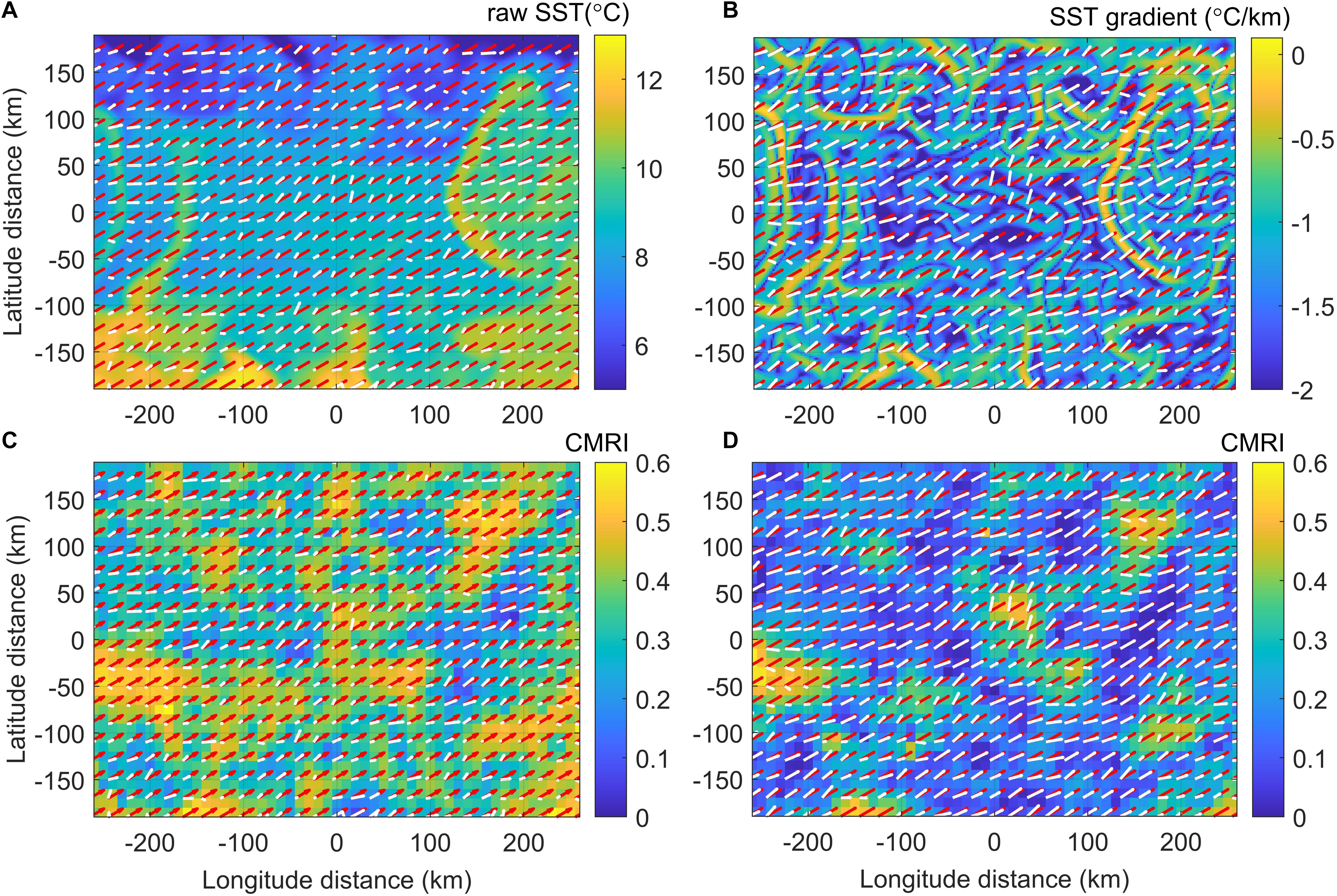
Figure 1. Example comparison of true velocity field V_true in a 10 km-grid (red arrows) and calculated velocity field V_cal in a 10 km-grid (white arrows) for raw SST (A) and SST gradient (B). Contours in panels (C,D) show CMRI errors corresponding to panels (A,B), respectively.

The relevant spatially varying error inevitably occurs by the PIV method that applies to the smooth scalar image that does not include noise-like particles whose scale is much smaller than the interrogation window. Even the scale of features revealed in the scalar field we have was comparable to the grid size of the velocity field. In this case, the PIV algorithm misleadingly interprets the movement of a unidirectional front to the direction normal to the front. The smaller the features in the scalar field, the lower the CMRI error. This can be simply examined by adding a noise before performing PIV: if a random noise (maximum magnitude at 5% of STD) was added to the first image (I₁), the CMRI error in Figures 1C,D were reduced by 10% for SST-R and 50% for SST-G.

Figure 2 shows spatially averaged errors (WRI, WMI, and CMRI) that vary with different angles and magnitudes of V_true for SST-R, SST-G, and SST-G² (second-order gradient). For the SST-R case, the difference between two consecutive images is less distinct, which increases the uncertainty in determining the displacement vector in the cross-correlation calculation. WRI (Figures 2A–C), WMI (Figures 2D–F), and CMRI (Figures 2G–I) indicate that taking the gradient of SST is advantageous for both vector alignment and magnitude estimations. Emery et al. (1986) qualitatively showed that using the SST gradient yields better results from raw SST; however, most works afterward utilized raw scalar fields to derive surface currents from satellite observations (Yang et al., 2014; Kim et al., 2016; Sun et al., 2016; Park et al., 2018; Choi et al., 2019). Nevertheless, when taking multiple gradients, the narrowing front becomes indistinguishable from random noise so that the error can be increased from the smallest grid size, as shown in Figures 2C,F,I.

FIGURE 2

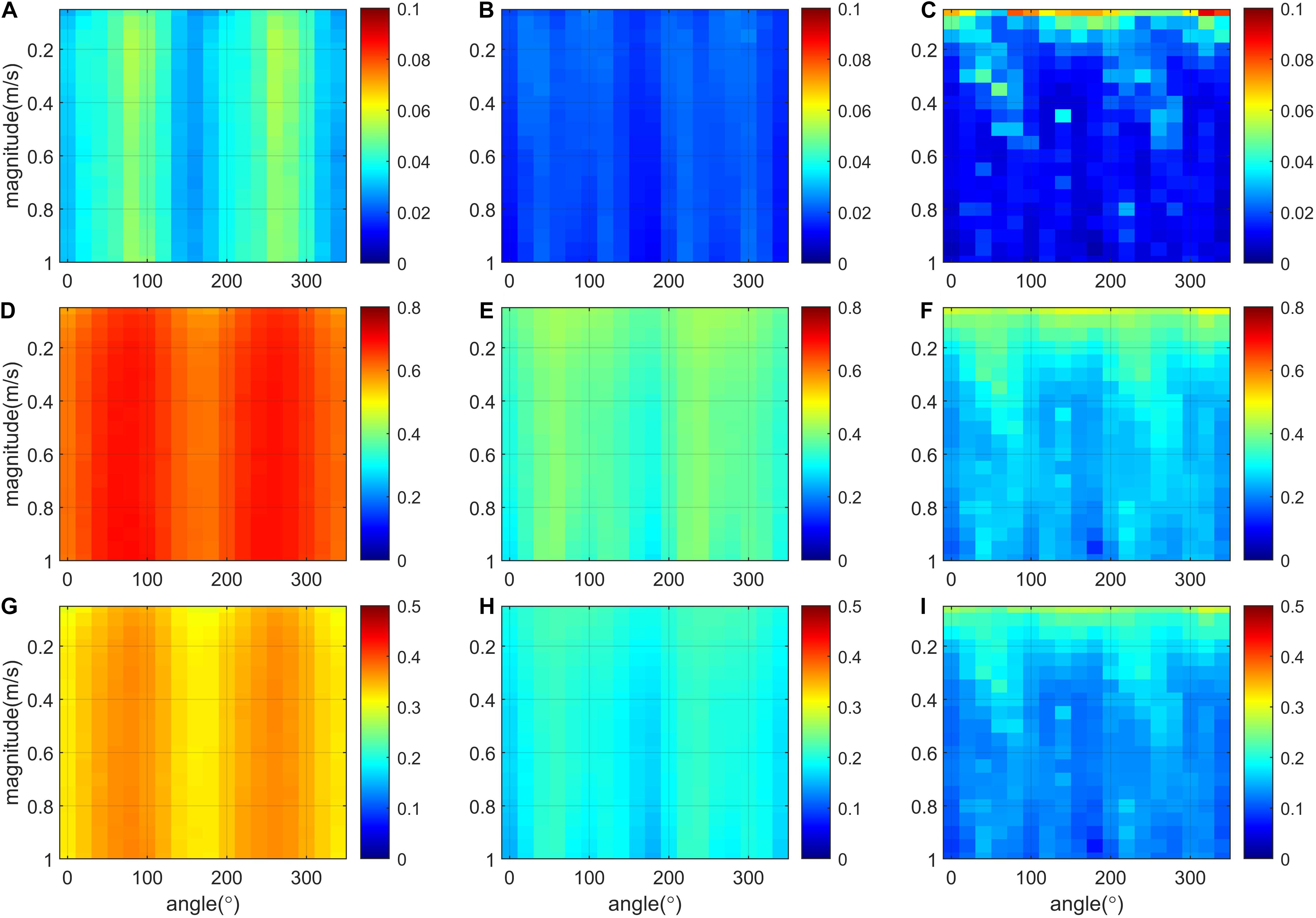
Figure 2. Spatially-averaged WRI (upper panels), WMI (middle panels), CMRI (lower panels) errors for SST-R (A,D,G), SST-G (B,E,H), and SST-G² (C,F,I) depending on the magnitude and direction of V_true. SST-R, SST-G, and SST-G² indicate surface current generated from the raw SST, the spatial gradient of raw SST, and the second order spatial gradient of raw SST, respectively.

The error is amplified near the angles around 90° and 270° (Figure 2A), and such observation indicates an anisotropy in the horizontal shape of mesoscale eddies and fronts that are elongated and aligned along the north–south direction over the East/Japan Sea, which appears more prominently in the WRI error. The spatial averages of CMRI were 0.34, 0.20, and 0.15 for SST-R, SST-G, and SST-G², respectively. Those for WRI (WMI) were 0.04, 0.02, and 0.02 (0.65, 0.37, and 0.28), respectively.

Convolutional Neural Network Training and Surface Current Evaluation

By applying the CNN to the training datasets SST-R and SST-G, we generated a network that classified the image difference into two classes, good and bad, based on the CMRI error. For the SST-R training dataset, the image difference for low CMRI < 0.3 and high CMRI > 0.4 were labeled as good and bad vectors, respectively, while for the SST-G training dataset, low CMRI < 0.1 and high CMRI > 0.3 were labeled as good and bad vectors (Supplementary Figure 3). The shape of the probability density function (PDF) of CMRI is skewed toward low CMRI for SST-R and Gaussian for SST-G. Those partitions were made to ensure the bad and good classes had similar amounts of data, and different datasets may have different partitions depending on the CMRI PDF. In most cases, images showing more coherent patterns are placed in the good class; however, the traits that lead a vector to be classified in the good or bad class are not determinable without performing deep learning-based examination. In this work, we trained only the SST-R and SST-G datasets for evaluating the surface current, and the final validation accuracies for those at 100 epochs were 85.8 and 89.7%, respectively. The accuracy and the results did not show significant changes after epoch 50.

Figure 3 shows the deep learning-based evaluation of the surface current using synthetic data generated simultaneously by SST and velocity fields on DOY 150 covering longitude 129°N–136.5°N and latitude 36.5°E–40.5°E in the OPEM model. The black and green vectors indicate the model surface current (V_true) and calculated surface current (V_cal), and the SST-R and SST-G datasets are sequentially displayed in Figures 3A,B. The background color of the figure is the CMRI error showing the deviation between V_true deforming the original image and V_cal obtained by applying PIV to the original image (I₁) and the deformed image (I₂). The blue circles designate the vectors within top 30% having high reliability evaluated by deep learning CNN. The pretrained deep learning network classified good vectors (blue circles shown in Figure 3), mostly at low CMRI values. To quantify the performance of the network, the correlation coefficient (r) between V_true and V_cal was calculated (Supplementary Figure 5). For SST-R, u and v velocity components showed r_u = 0.572 and r_v = 0.479 while applying the trained network gave r_u = 0.761 and r_v = 0.722. For SST-G, u and v velocity components showed r_u = 0.704 and r_v = 0.608 while applying the trained network gave r_u = 0.799 and r_v = 0.816. We also calculated the correlation coefficient between δ_true and δ_cal (divergence) using the same velocity fields. For SST-R, applying the network increased r_δ from 0.366 to 0.401, and for SST-G, applying the network increased r_δ from 0.514 to 0.550. Overall, the surface current involved with SST-G resulted in a lower CMRI error than that involved with SST-R, and the pretrained network using the SST-G dataset showed better performance in identifying good vectors.

FIGURE 3

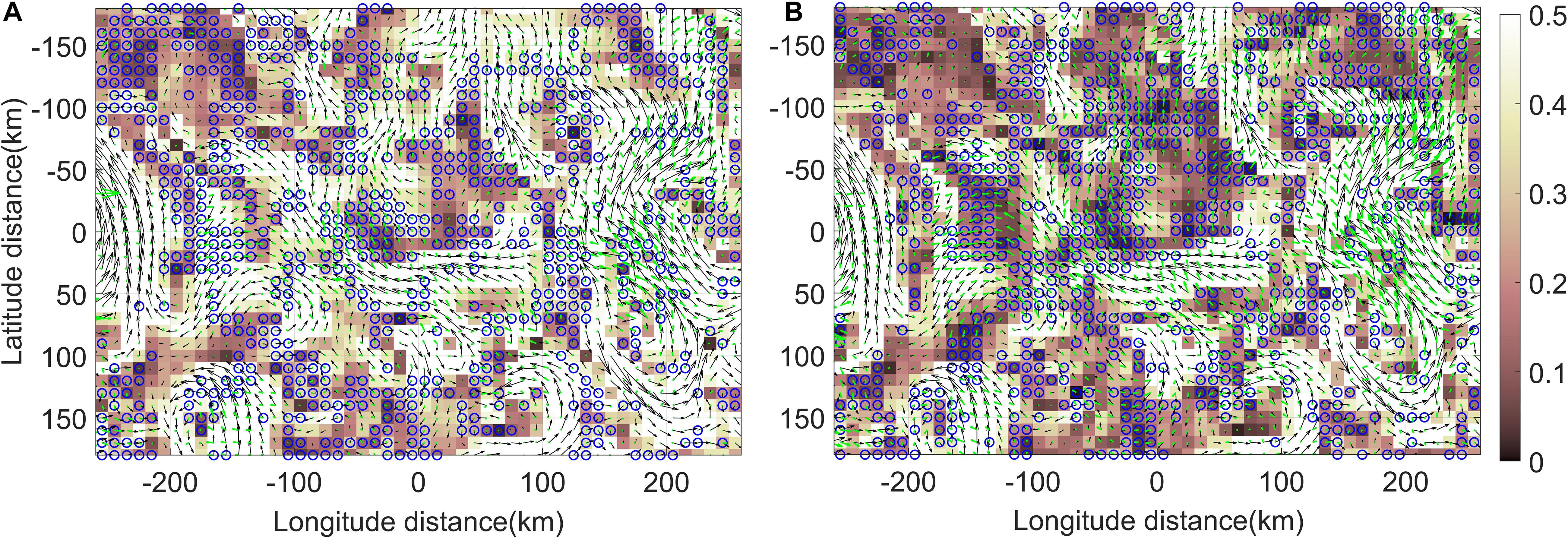
Figure 3. Surface current reliability determination based on CNN evaluation for SST-R (A) and SST-G (B). The black vector is the model surface current (true), and the green vector is the PIV surface current (calculated). The background color represents the difference (CMRI error) between the true value and the calculated value (0: lowest error / 1: highest error). The blue circles designate the vectors within top 30% having high reliability evaluated by deep learning CNN.

The same procedures of calculating the surface current and applying the deep learning pretrained network as above were implemented with the image pair of Himawari skin SST captured on March 25, 2018 over the area of the East/Japan Sea. We obtained V_cal in a 10-km resolution by applying PIV to two consecutive Himawari SST images in a 2-km resolution, and each vector was linked to a good or bad vector based on the evaluation by the deep learning network. Figure 4 shows the 1-day average of the hourly surface currents from hourly Himawari SST (Figure 4A) and the Himawari SST gradient (Figure 4B). Only vectors within the top 30% accuracy evaluated by the deep learning network at each snapshot were used for the average, and the field were smoothed by a 3 × 3 mean filter. The surface current generated by the SST gradient contains slightly stronger velocity and dynamic features such that more distinct eddies can be identified.

FIGURE 4

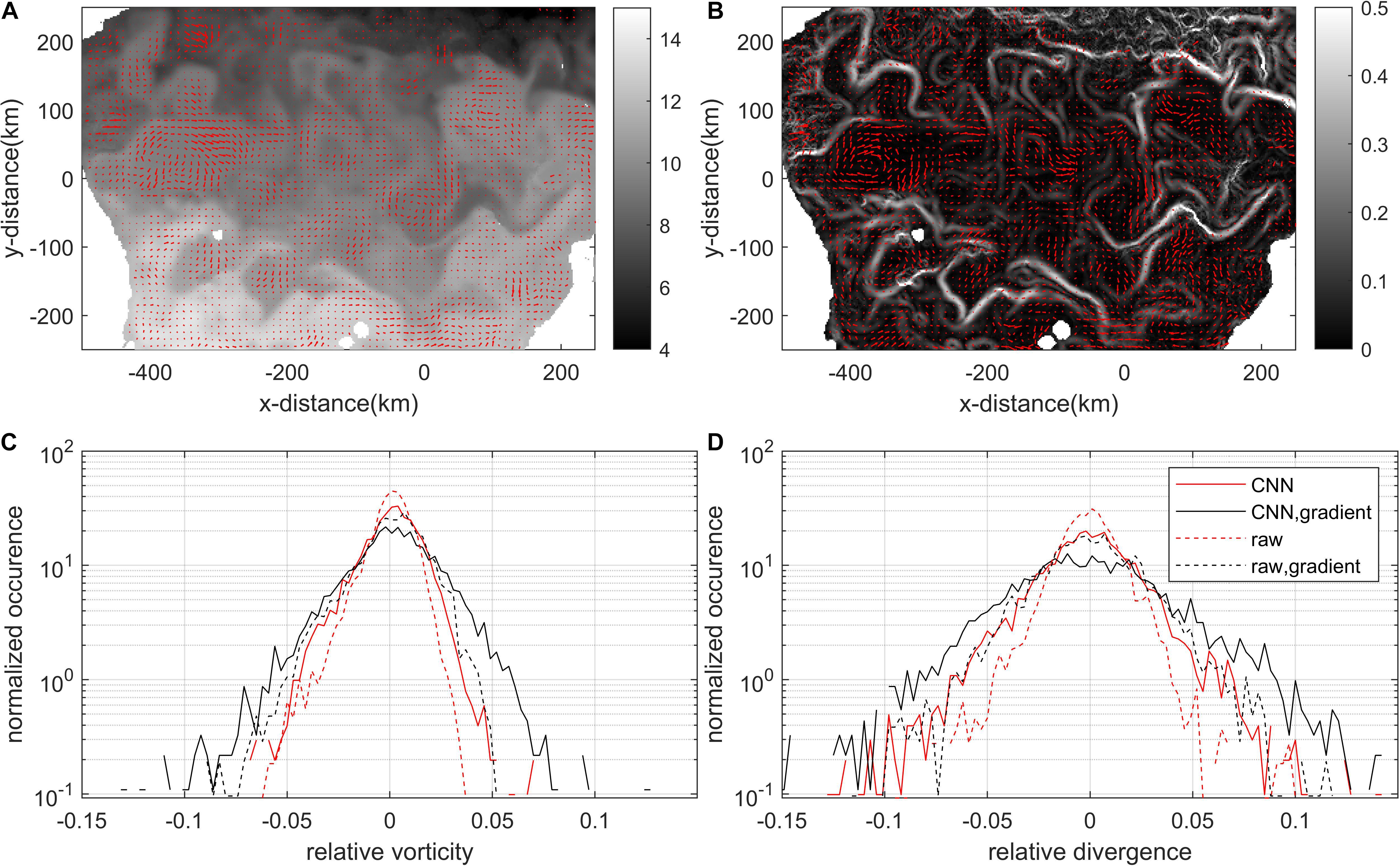
Figure 4. One-day averaged surface current in a 10 km-grid in the East/Japan Sea on 25th March 2018 derived from Himawari SST (A) and Himawari SST gradient (B) and corresponding scalar fields. 22 hourly velocity fields derived from 23 consecutive SST images were used to calculate the mean surface current for that date. The scattered cloud area accounted for about 68%, and the area excluding the cloud area was used to calculate the mean velocity field. (C,D) Indicate vorticity and divergence PDF normalized by local Coriolis parameter. In the legend, “CNN” indicates 1-day averaged surface current using vectors filtered by CNN, “raw” indicates 1-day averaged surface current without CNN filtering, and “gradient” indicates surface current derived from SST gradient. The standard derivation (STD) of the PDF are 0.0158 (CNN), 0.0254 (CNN-gradient), 0.0117 (raw), and 0.0183 (raw-gradient) for relative vorticity, and 0.0288 (CNN), 0.0420 (CNN-gradient), 0.0181 (raw), and 0.0284 (raw-gradient) for relative divergence. The changes in STD show that flatter PDF (or smaller circulations) can be obtained by CNN-filtering and taking gradient of a scalar field.

Figures 4C,D show the PDFs of the vorticity (Figure 4C) and divergence (Figure 4D) fields normalized by the Coriolis parameter. The PDFs calculated from the PIV-derived current with CNN filtering (solid red lines) have heavier or flatter tails than the ones from the PIV-derived current without the CNN filtering (dashed red lines), and taking the gradient (black lines) also leads the tails to be flatter. Since heavier tail in a divergence and vorticity PDFs is indicative of realizing smaller-scale features (or stronger submesoscale circulations) (Barkan et al., 2017; Choi et al., 2017), it is considered that taking gradients of a scalar field along with filtering the vectors through CNN evaluation are considered helpful in realizing smaller features in the surface current. Due to the limited grid size of surface currents, the sub-grid circulations with a size less than 10 km cannot be considered in this study. However, applying the strategy to high-resolution scalar fields, such as 250 m-grid satellite products from the Geostationary Ocean Color Imager (GOCI), would provide submesoscale-resolving (∼3 km) features in surface currents.

Conclusion

The estimation of surface currents associated with geostationary satellite data, the PIV method, and deep learning networks has been conducted to suggest a strategy for the production of operational surface currents. Information of real-time surface currents can be very useful for practical and scientific applications. However, an operating system based on geostationary satellite observation that can cover marginal seas and sample at high spatiotemporal resolutions has not yet been developed.

We demonstrated the generation of surface currents from model SST. Applying PIV to the scalar field resulted in errors that were correlated with the direction of the front and true velocity field. To point out erroneous vectors, we conducted a deep learning-based evaluation of vectors, which was achieved by training the image difference between two consecutive scalar images. We found taking the gradient of the scalar field performed better in generating surface currents. We also applied the same procedure to Himawari SST to provide a quality flag indicating the surface current’s reliability. Based on the quality flag that evaluated each vector, good vectors were chosen and used to generate an averaged velocity field showing clear dynamics of coherent mesoscale eddies, which was confirmed by heavy tails in the PDFs of kinematics. Although a limited amount of training data was generated and used for deep learning training, the trained network successfully discerned more accurate vectors of the calculated surface currents.

The strategy introduced in this paper can be applied to not only the Himawari satellite but also the newly launched GOCI-II geostationary satellite that just started generating ocean color scalar fields in a 250-m grid. Furthermore, this study can be extended to produce vast synthetic data (model and experimental data) to develop a pretrained network that can give the right vector in numerous situations and can be applied to different kinds of scalar fields.

Data Availability Statement

The original contributions presented in the study are included in the article/Supplementary Material, further inquiries can be directed to the corresponding author/s.

Author Contributions

JC: plan research, write paragraphs, and data analysis. WK: write paragraphs and research advice. TH: write paragraphs and data analysis. Y-GP: plan research and research advice. All authors contributed to the article and approved the submitted version.

Funding

This work was funded through the projects “Investigation and prediction system development of marine heatwave around the Korean Peninsula originated from the subarctic and Western Pacific (20190344)” from the Ministry of Oceans and Fisheries, South Korea, and “Building Conceptual Design for Mid-size Integrated CCS Demonstration (20214710100060)” from the Korea Institute of Energy Technology Evaluation and Planning.

Conflict of Interest

The authors declare that the research was conducted in the absence of any commercial or financial relationships that could be construed as a potential conflict of interest.

Publisher’s Note

All claims expressed in this article are solely those of the authors and do not necessarily represent those of their affiliated organizations, or those of the publisher, the editors and the reviewers. Any product that may be evaluated in this article, or claim that may be made by its manufacturer, is not guaranteed or endorsed by the publisher.

Supplementary Material

The Supplementary Material for this article can be found online at: https://www.frontiersin.org/articles/10.3389/fmars.2021.695780/full#supplementary-material

Footnotes

1. ^ MATLAB and Deep Learning Toolbox Release 2021b, The MathWorks, Inc., Natick, MA.

References

Avallone, F., Ragni, D., Schrijer, F. F., Scarano, F., and Cardone, G. (2016). Study of a supercritical roughness element in a hypersonic laminar boundary layer. AIAA J. 54, 1892–1900. doi: 10.2514/1.J054610

PubMed Abstract | CrossRef Full Text | Google Scholar

Barkan, R., McWilliams, J. C., Shchepetkin, A. F., Molemaker, M. J., Renault, L., Bracco, A., et al. (2017). Submesoscale dynamics in the northern Gulf of Mexico. Part I: regional and seasonal characterization and the role of river outflow. J. Phys. Oceanogr. 47, 2325–2346. doi: 10.1175/JPO-D-17-0035.1

CrossRef Full Text | Google Scholar

Berta, M., Griffa, A., Magaldi, M. G., Özgökmen, T. M., Poje, A. C., Haza, A. C., et al. (2015). Improved surface velocity and trajectory estimates in the Gulf of Mexico from blended satellite altimetry and drifter data. J. Atmos. Ocean. Technol. 32, 1880–1901. doi: 10.1175/JTECH-D-14-00226.1

CrossRef Full Text | Google Scholar

Bjorck, J., Gomes, C., Selman, B., and Weinberger, K. Q. (2018). Understanding batch normalization. arXiv [Preprint]. arXiv:1806.02375

Google Scholar

Boccaletti, G., Ferrari, R., and Fox-Kemper, B. (2007). Mixed layer instabilities and restratification. J. Phys. Oceanogr. 37, 2228–2250. doi: 10.1175/JPO3101.1

CrossRef Full Text | Google Scholar

Bracco, A., Chassignet, E. P., Garraffo, Z. D., and Provenzale, A. (2003). Lagrangian velocity distributions in a high-resolution numerical simulation of the North Atlantic. J. Atmos. Ocean. Technol. 20, 1212–1220. doi: 10.1175/1520-04262003020<1212:LVDIAH<2.0.CO;2

CrossRef Full Text | Google Scholar

Breivik, Ø., and Allen, A. A. (2008). An operational search and rescue model for the Norwegian Sea and the North Sea. J. Mar. Syst. 69, 99–113. doi: 10.1016/j.jmarsys.2007.02.010

CrossRef Full Text | Google Scholar

Buesseler, K. O., Jayne, S. R., Fisher, N. S., Rypina, I. I., Baumann, H., Baumann, Z., et al. (2012). Fukushima-derived radionuclides in the ocean and biota off Japan. Proc. Natl. Acad. Sci. U.S.A. 109, 5984–5988. doi: 10.1073/pnas.1120794109/-/DCSupplemental

PubMed Abstract | CrossRef Full Text | Google Scholar

Cai, S., Zhou, S., Xu, C., and Gao, Q. (2019). Dense motion estimation of particle images via a convolutional neural network. Exp. Fluids 60:73. doi: 10.1007/s00348-019-2717-2

CrossRef Full Text | Google Scholar

Chattopadhyay, A., Hassanzadeh, P., and Pasha, S. (2020). Predicting clustered weather patterns: a test case for applications of convolutional neural networks to spatio-temporal climate data. Sci. Rep. 10:1317. doi: 10.1038/s41598-020-57897-9

PubMed Abstract | CrossRef Full Text | Google Scholar

Choi, J., Bracco, A., Barkan, R., Shchepetkin, A. F., McWilliams, J. C., and Molemaker, J. M. (2017). Submesoscale dynamics in the northern Gulf of Mexico. Part III: Lagrangian implications. J. Phys. Oceanogr. 47, 2361–2376. doi: 10.1175/JPO-D-17-0036.1

CrossRef Full Text | Google Scholar

Choi, J., Park, Y. G., Kim, W., and Kim, Y. H. (2019). Characterization of submesoscale turbulence in the East/Japan sea using geostationary ocean color satellite images. Geophys. Res. Lett. 46, 8214–8223. doi: 10.1029/2019GL083892

CrossRef Full Text | Google Scholar

Corrado, R., Lacorata, G., Palatella, L., Santoleri, R., and Zambianchi, E. (2017). General characteristics of relative dispersion in the ocean. Sci. Rep. 7:46291. doi: 10.1038/srep46291

PubMed Abstract | CrossRef Full Text | Google Scholar

Dalziel, J., and Pelot, R. (2019). “Maritime emergency preparedness and management,” in The Future of Ocean Governance and Capacity Development (Leiden: Brill Nijhoff), 473–478. doi: 10.1163/9789004380271_082

CrossRef Full Text | Google Scholar

Dohan, K. (2017). Ocean surface currents from satellite data. J. Geophys. Res. Oceans 122, 2647–2651. doi: 10.1002/2017JC012961

CrossRef Full Text | Google Scholar

Dohan, K., and Maximenko, N. (2010). Monitoring ocean currents with satellite sensors. Oceanography 23, 94–103. doi: 10.5670/oceanog.2010.08

CrossRef Full Text | Google Scholar

Donlon, C. J., Minnett, P. J., Gentemann, C., Nightingale, T. J., Barton, I. J., Ward, B., et al. (2002). Toward improved validation of satellite sea surface skin temperature measurements for climate research. J. Clim. 15, 353–369. doi: 10.1175/1520-04422002015<0353:TIVOSS<2.0.CO;2

CrossRef Full Text | Google Scholar

Emery, W. J., Thomas, A. C., Collins, M. J., Crawford, W. R., and Mackas, D. L. (1986). An objective method for computing advective surface velocities from sequential infrared satellite images. J. Geophys. Res. Oceans 91, 12865–12878. doi: 10.1029/JC091iC11p12865

CrossRef Full Text | Google Scholar

Guo, T., Dong, J., Li, H., and Gao, Y. (2017). “Simple convolutional neural network on image classification,” in Proceedings of the 2017 IEEE 2nd International Conference on Big Data Analysis (ICBDA), (Piscataway, NJ: IEEE), 721–724.

Google Scholar

Ham, Y. G., Kim, J. H., and Luo, J. J. (2019). Deep learning for multi-year ENSO forecasts. Nature 573, 568–572. doi: 10.5281/zenodo.3244463

CrossRef Full Text | Google Scholar

Huntingford, C., Jeffers, E. S., Bonsall, M. B., Christensen, H. M., Lees, T., and Yang, H. (2019). Machine learning and artificial intelligence to aid climate change research and preparedness. Environ. Res. Lett. 14:124007. doi: 10.1088/1748-9326/ab4e55

CrossRef Full Text | Google Scholar

Iwasaki, S., Isobe, A., Kako, S. I., Uchida, K., and Tokai, T. (2017). Fate of microplastics and mesoplastics carried by surface currents and wind waves: a numerical model approach in the Sea of Japan. Mar. Pollut. Bull. 121, 85–96. doi: 10.1016/j.marpolbul.2017.05.057

PubMed Abstract | CrossRef Full Text | Google Scholar

Kim, W., Moon, J. E., Park, Y. J., and Ishizaka, J. (2016). Evaluation of chlorophyll retrievals from Geostationary Ocean color imager (GOCI) for the north-east Asian region. Remote Sens. Environ. 184, 482–495. doi: 10.1016/j.rse.2016.07.031

CrossRef Full Text | Google Scholar

Kim, Y. H., Hwang, C., and Choi, B. J. (2015). An assessment of ocean climate reanalysis by the data assimilation system of KIOST from 1947 to 2012. Ocean Model. 91, 1–22. doi: 10.1016/j.ocemod.2015.02.006

CrossRef Full Text | Google Scholar

Kurihara, Y., Murakami, H., and Kachi, M. (2016). Sea surface temperature from the new Japanese geostationary meteorological Himawari−8 satellite. Geophys. Res. Lett. 43, 1234–1240. doi: 10.1002/2015GL067159

CrossRef Full Text | Google Scholar

Kwon, K., Choi, B. J., Kim, K. Y., and Kim, K. (2019). Tracing the trajectory of pelagic Sargassum using satellite monitoring and Lagrangian transport simulations in the East China Sea and Yellow Sea. Algae 34, 315–326. doi: 10.4490/algae.2019.34.12.11

CrossRef Full Text | Google Scholar

LaCasce, J. (2008). Statistics from Lagrangian observations. Prog. Oceanogr. 77, 1–29. doi: 10.1016/j.pocean.2008.02.002

CrossRef Full Text | Google Scholar

Lancewicki, T., and Kopru, S. (2019). Automatic and simultaneous adjustment of learning rate and momentum for stochastic gradient descent. arXiv [Preprint]. arXiv:1908.07607

Google Scholar

Laxague, N. J., Özgökmen, T. M., Haus, B. K., Novelli, G., Shcherbina, A., Sutherland, P., et al. (2018). Observations of near−surface current shear help describe oceanic oil and plastic transport. Geophys. Res. Lett. 45, 245–249. doi: 10.1002/2017GL075891

CrossRef Full Text | Google Scholar

Leese, J. A., Novak, C. S., and Clark, B. B. (1971). An automated technique for obtaining cloud motion from geosynchronous satellite data using cross correlation. J. Appl. Meteorol. Climatol. 10, 118–132. doi: https://doi.org/10.1175/1520-0450(1971)010<0118:AATFOC>2.0.CO;2

CrossRef Full Text | Google Scholar

Legleiter, C. J., Kinzel, P. J., and Nelson, J. M. (2017). Remote measurement of river discharge using thermal particle image velocimetry (PIV) and various sources of bathymetric information. J. Hydrol. 554, 490–506. doi: 10.1016/j.jhydrol.2017.09.004

CrossRef Full Text | Google Scholar

Liu, F., Zhou, Z., Samsonov, A., Blankenbaker, D., Larison, W., Kanarek, A., et al. (2018). Deep learning approach for evaluating knee MR images: achieving high diagnostic performance for cartilage lesion detection. Radiology 289, 160–169. doi: 10.1148/radiol.2018172986

PubMed Abstract | CrossRef Full Text | Google Scholar

Lou, R., Lv, Z., Dang, S., Su, T., and Li, X. (2021). Application of machine learning in ocean data. Multimed. Syst. 1–10. doi: 10.1007/s00530-020-00733-x

CrossRef Full Text | Google Scholar

Lumpkin, R., and Pazos, M. (2007). “Measuring surface currents with surface velocity program drifters: the instrument, its data, and some recent results,” in Lagrangian Analysis and Prediction of Coastal and Ocean Dynamics, Vol. 39, eds A. Griffa, A. D. Kirwan, A. J. Mariano, T. Özgökmen, and H. T. Rossby (Cambridge: Cambridge University Press), 67. doi: 10.1017/CBO9780511535901.003

CrossRef Full Text | Google Scholar

Mahadevan, A. (2016). The impact of submesoscale physics on primary productivity of plankton. Annu. Rev. Mar. Sci. 8, 161–184. doi: 10.1146/annurev-marine-010814-015912

PubMed Abstract | CrossRef Full Text | Google Scholar

McNutt, M. K., Camilli, R., Crone, T. J., Guthrie, G. D., Hsieh, P. A., Ryerson, T. B., et al. (2012). Review of flow rate estimates of the Deepwater Horizon oil spill. Proc. Natl. Acad. Sci. U.S.A. 109, 20260–20267. doi: 10.1073/pnas.1112139108

PubMed Abstract | CrossRef Full Text | Google Scholar

Molemaker, M. J., McWilliams, J. C., and Capet, X. (2010). Balanced and unbalanced routes to dissipation in an equilibrated Eady flow. J. Fluid Mech. 654, 35–63. doi: 10.1017/S0022112009993272

CrossRef Full Text | Google Scholar

Osadchiev, A., and Sedakov, R. (2019). Spreading dynamics of small river plumes off the northeastern coast of the Black Sea observed by Landsat 8 and Sentinel-2. Remote Sens. Environ. 221, 522–533. doi: 10.1016/j.rse.2018.11.043

CrossRef Full Text | Google Scholar

Park, K. A., Lee, M. S., Park, J. E., Ullman, D., Cornillon, P. C., and Park, Y. J. (2018). Surface currents from hourly variations of suspended particulate matter from Geostationary Ocean Color Imager data. Int. J. Remote Sens. 39, 1929–1949. doi: 10.1080/01431161.2017.1416699

CrossRef Full Text | Google Scholar

Pinaya, W. H. L., Vieira, S., Garcia-Dias, R., and Mechelli, A. (2020). “Convolutional neural networks,” in Machine learning (Cambridge, MA: Academic Press), 173–191. doi: 10.1016/B978-0-12-815739-8.00010-9

CrossRef Full Text | Google Scholar

Rocha, C. B., Chereskin, T. K., Gille, S. T., and Menemenlis, D. (2016). Mesoscale to submesoscale wavenumber spectra in Drake Passage. J. Phys. Oceanogr. 46, 601–620. doi: 10.1175/JPO-D-15-0087.1

CrossRef Full Text | Google Scholar

Rypina, I. I., Kirincich, A. R., Limeburner, R., and Udovydchenkov, I. A. (2014). Eulerian and Lagrangian correspondence of high-frequency radar and surface drifter data: effects of radar resolution and flow components. J. Atmos. Ocean. Technol. 31, 945–966. doi: 10.1175/JTECH-D-13-00146.1

CrossRef Full Text | Google Scholar

Santiago, J. G., Wereley, S. T., Meinhart, C. D., Beebe, D. J., and Adrian, R. J. (1998). A particle image velocimetry system for microfluidics. Exp. Fluids 25, 316–319. doi: 10.1007/s003480050235

CrossRef Full Text | Google Scholar

Sklar, F. H., and Browder, J. A. (1998). Coastal environmental impacts brought about by alterations to freshwater flow in the Gulf of Mexico. Environ. Manag. 22, 547–562. doi: 10.1007/s002679900127

PubMed Abstract | CrossRef Full Text | Google Scholar

Sun, H., Song, Q., Shao, R., and Schlicke, T. (2016). Estimation of sea surface currents based on ocean colour remote-sensing image analysis. Int. J. Remote Sens. 37, 5105–5121. doi: 10.1080/01431161.2016.1226526

CrossRef Full Text | Google Scholar

Thielicke, W. (2014). The Flapping Flight of Birds – Analysis and Application. Ph.D. thesis. Groningen: Rijksuniversiteit.

Google Scholar

Thielicke, W., and Sonntag, R. (2021). Particle image velocimetry for MATLAB: accuracy and enhanced algorithms in PIVlab. J. Open Res. Softw. 9:12. doi: 10.5334/jors.334

CrossRef Full Text | Google Scholar

Thielicke, W., and Stamhuis, E. J. (2014). PIVlab – towards user-friendly, affordable and accurate digital particle image velocimetry in MATLAB. J. Open Res. Softw. 2:e30. doi: http://dx.doi.org/10.5334/jors.bl

CrossRef Full Text | Google Scholar

Tokumaru, P. T., and Dimotakis, P. E. (1995). Image correlation velocimetry. Exp. Fluids 19, 1–15. doi: 10.1007/BF00192228

CrossRef Full Text | Google Scholar

Walker, N. D., Wiseman, W. J., Rouse, L. J., and Babin, A. (2005). Effects of river discharge, wind stress, and slope eddies on circulation and the satellite-observed structure of the Mississippi River plume. J. Coast. Res. 21, 1228–1244. doi: 10.2112/04-0347.1

CrossRef Full Text | Google Scholar

Wereley, S. T., and Meinhart, C. D. (2010). Recent advances in micro-particle image velocimetry. Annu. Rev. Fluid Mech. 42, 557–576. doi: 10.1146/annurev-fluid-121108-145427

CrossRef Full Text | Google Scholar

Willman, C., Scott, B., Stone, R., and Richardson, D. (2020). Quantitative metrics for comparison of in-cylinder velocity fields using particle image velocimetry. Exp. Fluids 61:146. doi: 10.1007/s00348-020-2897-9

CrossRef Full Text | Google Scholar

Xu, D., and Chen, J. (2013). Accurate estimate of turbulent dissipation rate using PIV data. Exp. Ther. Fluid Sci. 44, 662–672. doi: 10.1016/j.expthermflusci.2012.09.006

CrossRef Full Text | Google Scholar

Yang, H., Choi, J. K., Park, Y. J., Han, H. J., and Ryu, J. H. (2014). Application of the Geostationary Ocean Color Imager (GOCI) to estimates of ocean surface currents. J. Geophys. Res. Oceans 119, 3988–4000. doi: 10.1002/2014JC009981

CrossRef Full Text | Google Scholar

Yanovsky, I., Holt, B., and Ayoub, F. (2020). “Deriving velocity fields of submesoscale eddies using multi-sensor imagery,” in Proceedings of the IGARSS 2020-2020 IEEE International Geoscience and Remote Sensing Symposium, (Piscataway, NJ: IEEE), 1921–1924. doi: 10.1109/IGARSS39084.2020.9323797

CrossRef Full Text | Google Scholar

Yoo, J. G., Kim, S. Y., and Kim, H. S. (2018). Spectral descriptions of submesoscale surface circulation in a coastal region. J. Geophys. Res. Oceans 123, 4224–4249. doi: 10.1029/2016JC012517

CrossRef Full Text | Google Scholar

Zavialov, P. O., Grigorieva, J. V., Möller, O. O. Jr., Kostianoy, A. G., and Gregoire, M. (2002). Continuity preserving modified maximum cross−correlation technique. J. Geophys. Res. Oceans 107:3160. doi: 10.1029/2001JC001116

CrossRef Full Text | Google Scholar