Exploring Ocean Biogeochemistry Using a Lab-on-Chip Phosphate Analyser on an Underwater Glider

Introduction

The ocean phosphorus biogeochemical cycle is intrinsically linked with the cycles of carbon, oxygen, nitrogen, sulfur, silicon, and trace metals (Moore et al., 2013; Karl, 2014). The temporal scales of the processes acting upon the ocean phosphorus cycle range from hours to weeks (e.g., gene expression and microbial growth), months to decades (e.g., biological carbon pump and ocean circulation), and hundreds of years to millennia (e.g., tectonics and sedimentation) (Moore et al., 2013; Karl, 2014). Therefore, in order to understand and quantify the processes acting upon the ocean phosphorus cycle, oceanographers must make accurate and precise measurements over a range of temporal and spatial scales.

In oceanographic studies, the most commonly measured chemical form of phosphorus is phosphate (PO₄^3–). PO₄^3– concentrations are traditionally determined following manual sampling of seawater; water is collected at known times and depths, filtered (0.20 or 0.45 μm), and then preserved for laboratory analysis on board ships or on land (Jońca et al., 2013). There are numerous sample preservation approaches available for nutrient analysis; these include filtration, heating, pasteurisation, refrigeration, freezing and chemical poisoning, with diverse recommendations found in the literature (Clementson and Wayte, 1992; Dore et al., 1996; Aminot and Kérouel, 1997; Kattner, 1999; Gardolinski et al., 2001). Consequently, selecting an appropriate preservation method is non-trivial, and has been shown to be dependent upon the physico-chemical properties of the sample (e.g., salinity, calcium content, organic matter content) (Burton, 1973; Gardolinski et al., 2001). The most common method for measuring PO₄^3– is coupling the phosphomolybdenum blue (PMB) spectrophotometric assay with a gas-segmented continuous-flow analyser (Murphy and Riley, 1962; Hydes et al., 2010; Worsfold et al., 2016).

In situ techniques enhance the spatial and temporal resolution and coverage, providing marine chemists with a more detailed insight into biogeochemical cycling, and enhance monitoring capabilities (Daniel et al., 2020). Additionally, in situ techniques remove the need for sample preservation (Nightingale et al., 2015), which is a considerable advantage. Several attempts have been made to develop in situ systems capable of measuring PO₄^3– in natural waters using compact flow injection manifolds and microfluidic Lab-on-Chip (LoC) analysers (Lyddy-Meaney et al., 2002; Thouron et al., 2003; Adornato et al., 2007; Slater et al., 2010; Legiret et al., 2013; Clinton-Bailey et al., 2017; Grand et al., 2017) and electrochemical techniques (Jońca et al., 2011; Barus et al., 2016). Flow injection systems utilising miniaturised peristaltic pumps may suffer from drifting flow rates as tubing wears out and mechanical parts fail during prolonged usage. These systems require relatively large power sources, limiting them either to short deployments or deployments at locations with an external power supply (Nightingale et al., 2015). Electrochemical PO₄^3– sensor prototypes under development have the potential to offer small, low power, and reagent free detection. However, current prototypes are not sufficiently developed for large scale use (Jońca et al., 2013; Daniel et al., 2020; Wei et al., 2021).

Microfluidic technology involves the miniaturisation of analytical methods, typically using channels with cross-sectional dimensions below 1 mm and low flow rates (μL/min to mL/min). Their characteristic low volumes reduce the consumption of reagents and generation of waste and require little power to actuate the movement of fluids. LoC nutrient analysers with power consumption below 2 W have been demonstrated (Cleary et al., 2010; Beaton et al., 2011, 2012; Clinton-Bailey et al., 2017; Grand et al., 2017). Currently the application of PO₄^3– measuring microfluidic technology has been largely restricted to fluvial, waste water or estuarine environments (Cleary et al., 2010; Cohen et al., 2013; Gilbert et al., 2013; Clinton-Bailey et al., 2017). Marine deployments have been reported on fixed moorings, underway ship pumped systems, and a YOYO profiler (Thouron et al., 2003; Legiret et al., 2013; Grand et al., 2017).

In this study, we integrate a microfluidic LoC PO₄^3– analyser into an underwater glider (Kongsberg Seaglider) to determine PO₄^3– concentrations in the northern North Sea as part of the AlterEco programme (An alternative framework to assess marine ecosystem functioning in shelf seas, NERC reference NE/P013902/2). The LoC analyser used in this study was developed at the National Oceanography Centre (NOC), United Kingdom (Clinton-Bailey et al., 2017; Grand et al., 2017). A comparison of the specifications of the NOC analyser and the commercially available Sea-Bird Scientific HydroCycle-PO₄ is presented in Table 1. A number of features make the NOC analyser ideal for integration with gliders or other autonomous underwater vehicles (AUVs); the relatively compact size and small waste generation require minimal payload space; its pressure compensating housing permits regular profiling over depth, down to 6,000 m; low power requirements provide maximum endurance; high sampling frequency (5 samples per hour in the Seaglider configuration described here) allows for resolution of changes in nutrient concentrations occurring over small spatial scales, such as across a thermocline. The analytical figures of merit (accuracy, precision, limit of detection, and quantification) allow for the determination of PO₄^3– concentrations in all but the most oligotrophic regions of the ocean, and in situ results have been validated using water samplers and benchtop spectrophotometric reference methods (Grand et al., 2017). The combined (random and systematic uncertainty) measurement uncertainty associated with LoC PO₄^3– measurements from multiple LoC analysers was estimated to be 6.1% (u_c) (Birchill et al., 2019a).

TABLE 1

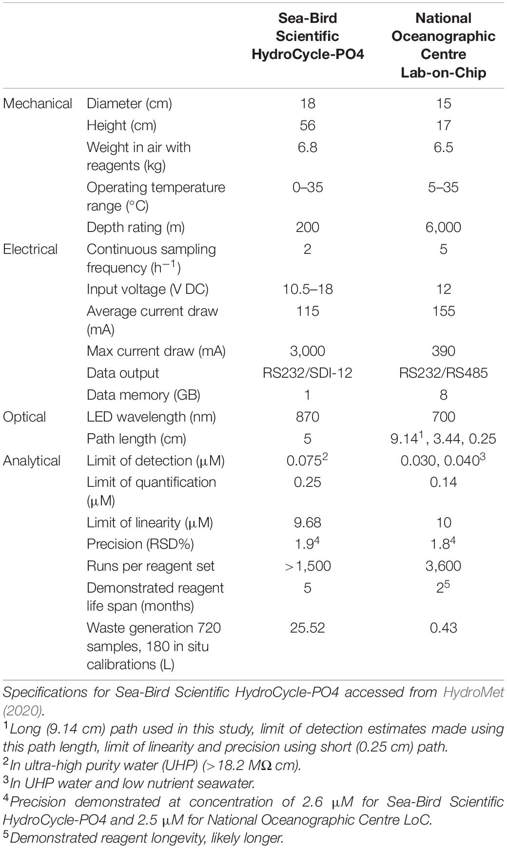
Table 1. Comparison of Sea-Bird Scientific HydroCycle-PO4 commercially available analyser and the National Oceanographic Centre, Lab-on-Chip analyser (AUV integration set up specifications).

To our knowledge, this study is the first report of in situ ocean PO₄^3– measurements conducted using an AUV. The potential for long term deployments make the LoC-glider approach appealing to both academic and marine management communities, enabling resolution of spatial and temporal scales that would be difficult and comparatively expensive to replicate using traditional shipboard studies (Liblik et al., 2016; Rudnick, 2016; Vincent et al., 2018). This manuscript provides a critical assessment of the first in situ PO₄^3– LoC–AUV deployment, considers potential future applications, and highlights development priorities.

Materials and Methods

Phosphomolybdenum Blue Spectrophotometric Assay

The PMB spectrophotometric assay is often coupled with gas-segmented continuous-flow analysers to make PO₄^3– concentration measurements in oceanographic studies (Hydes et al., 2010; Worsfold et al., 2016). The PO₄^3– LoC analyser used in this study also utilises the PMB assay. The PMB reaction follows two steps; (1) the formation of a Keggin ion around the analyte anion, and (2) the reduction of this heteropoly acid to form a blue coloured product (Nagul et al., 2015) (Eqs 1, 2).

${\text{PO}}_4^{3-}+12\mathrm{M}\mathrm{o}{\mathrm{O}}_4^{2-}+27{\mathrm{H}}^{+}\to {\text{H}}_3{\text{PO}}_4{\left({\text{MoO}}_3\right)}_{12}+12{\mathrm{H}}_2\text{O}(1)$

${\text{H}}_3{\text{PO}}_4{\left({\text{Mo}}^{\text{VI}}{\text{O}}_3\right)}_{12}+4{\mathrm{e}}^{-}+{\text{H}}^{+}\to {[{\text{H}}_4{\text{PMo}}_8^{\text{VI}}{\text{Mo}}_4^{\text{V}}{\text{O}}_{40}]}^{3-}(2)$

The key parameters to consider when utilising this colourimetric reaction are the molybdate and acid concentrations and choice of acid and reductant. Measurements made using this approach are commonly reported as orthophosphate (PO₄^3–, which also includes HPO₄^2–, H₂PO₄^–, and H₃PO₄; the dominant form in seawater at pH = 8 is HPO₄^2–) measurements. However, it is well established that the PMB complex may also be formed with acid labile, molybdate reactive organic P species, condensed polyphosphates and colloidal P (Burton, 1973; Nagul et al., 2015; Worsfold et al., 2016), thus the fraction accessed is more accurately defined as “soluble (molybdate) reactive phosphorus.” Magnesium coprecipitation allows for the isolation and concentration of inorganic P species prior to acidification. Detection following magnesium concentration therefore reduces the analytical interference caused by hydrolysis of organic P compounds. Application of the magnesium coprecipitation method to oligotrophic Pacific Ocean surface seawater consistently resulted in lower PO₄^3– concentrations (up to 50%) than concurrent analysis by traditional gas-segmented-continuous-flow techniques (Thomson-Bulldis and Karl, 1998). Consequently, a significant fraction of the apparent PO₄^3– signal observed in oligotrophic surface waters by result from P species other than PO₄^3–. Here, we refer to this operationally defined fraction as PO₄^3– to avoid confusion with the wider oceanographic literature.

Lab-on-Chip Analyser Description

The LoC PO₄^3– analyser used in this study was designed and fabricated at the National Oceanography Centre, United Kingdom (Figure 1). It is a slightly modified version (see section “Lab-on-Chip Analytical Cycle”) of the sensor that is described by Grand et al. (2017) and Clinton-Bailey et al. (2017). A detailed technical description can be found in the supporting information. Briefly, the LoC analyser is composed of a three layer poly(methyl methacrylate) chip with precision milled microchannels, mixers, and optical components consisting of light emitting diodes and photodiodes, electronics, solenoid valves, and syringe pumps mounted on the chip. The chip forms the end cap of a dark watertight pressure compensating PVC housing, which is rated to 6,000 dbar. Previous studies using the same LoC analyser as in this study demonstrated good agreement between in situ values and traditional shipboard and laboratory measurement techniques, with a limit of detection (3σ of 10 blank measurements) of 0.04 μM and limit of quantification (10σ of 10 blank measurements) of 0.14 μM (Clinton-Bailey et al., 2017; Grand et al., 2017).

FIGURE 1

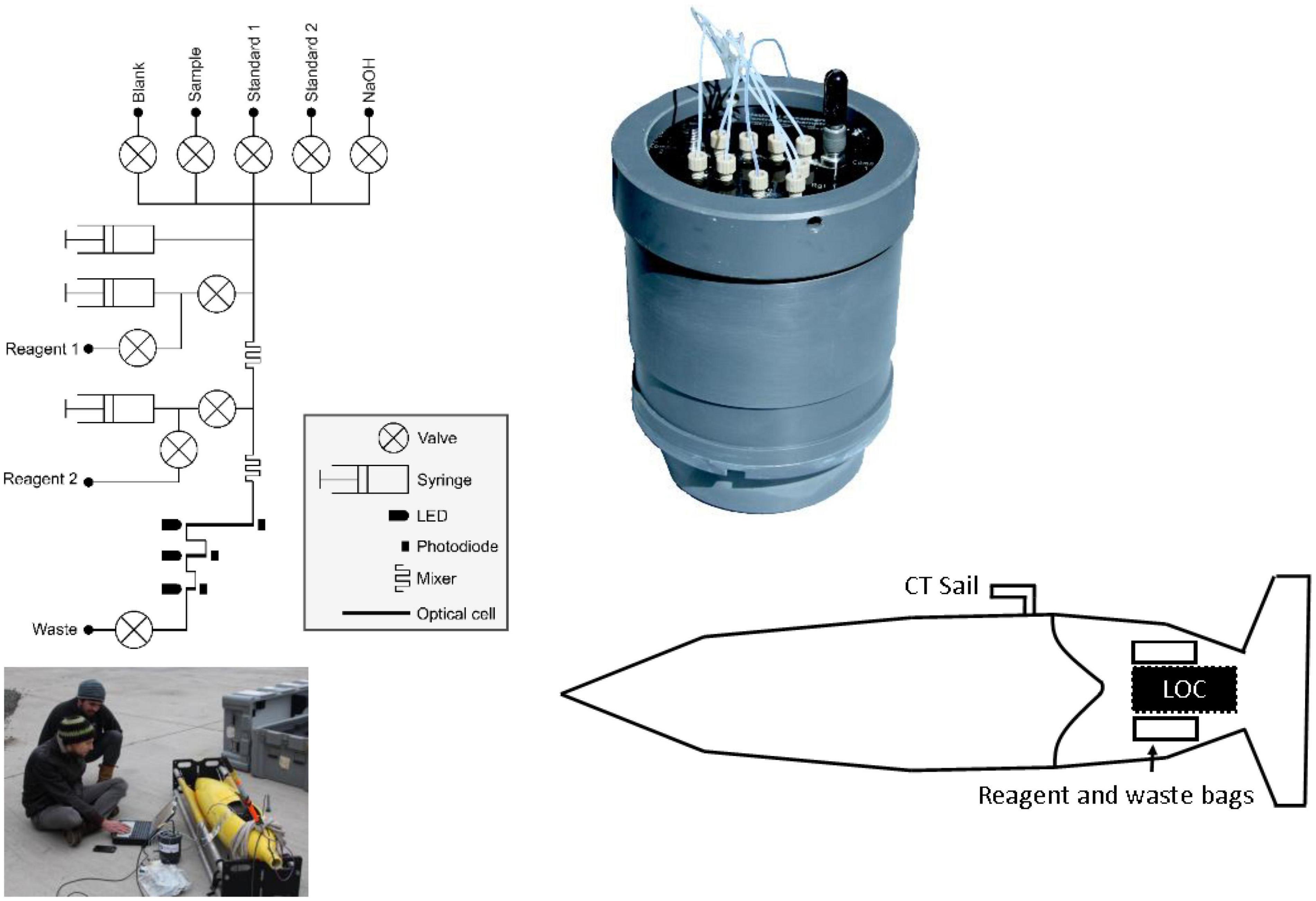
Figure 1. Fluidic diagram of the phosphate Lab-on-Chip analyser, picture of integration into glider Ogive faring, schematic showing location of analyser and reagent bags with the Seaglider (not to scale) and a close-up picture of the Lab-on-Chip analyser in pressure compensating housing.

The system is automated using a 32 bit microcontroller-based electronics package with 18-bit analogue to digital inputs and can stream raw data (1 Hz) over USB, as well as store data on a 8 GB flash memory card. Provided with the values of the on-board standards, the LoC analyser is capable of outputting processed data (μM PO₄^3–) over RS232 or RS485 interfaces. Transmitting only the processed data (i.e., not the raw data) reduces the size of near-real time data files, lessening the transmission duration and cost for satellite communications during an AUV deployment. Raw data is stored on an internal flash memory card, providing backup and access upon recovery.

Lab-on-Chip Reagent Preparation and Storage

Ultra-high purity water (UHP; 18.2 MΩ cm) was used for artificial seawater (ASW) standards and reagents. All plastic and glassware used to prepare reagents and standards was cleaned in 10% hydrochloric acid for 24 h, rinsed with UHP water and dried before use. All working solutions, including waste, were stored in flexible bags (FlexBoy, Sartorius-Stedim) inside the Ogive faring of the Seaglider during deployment.

The reagent preparation followed the procedure detailed by Grand et al. (2017). Briefly, the molybdate reagent (reagent 1) was made up of ammonium heptamolybdate tetrahydrate (0.45 mM), sulfuric acid (120 mM) and potassium antimonyl tartrate (0.06 mM). The reagent 1 storage bag was covered with opaque tape to prevent photodegradation of the chemicals before deployment inside the glider. The reducing reagent (reagent 2) was made up of L-ascorbic acid (0.057 M) and polyvinylpyrrolidone (0.1 g/L). The wash solution was made up of sodium hydroxide (NaOH; 0.01 M).

Blank and standard solutions were prepared in ASW to match the refractive index of seawater. ASW was prepared by dissolving sodium chloride (NaCl; 0.60 M; VWR, ACS reagent) and sodium bicarbonate (NaHCO₃; 0.006 M; Fisher, analytical grade reagent) in UHP water. To maintain PO₃^4– in solution whilst in the storage bags, blank, and standard solutions were acidified with sulfuric acid (H₂SO₄; 0.016 M; Fluka) (Clinton-Bailey et al., 2017). To prepare the standard solutions, a known amount of PO₄^3– was added. First, a 1 mM PO₄^3– stock was prepared by dissolving potassium phosphate monobasic salt (KH₂PO₄; 99+%, extra pure, Acros Organics) in UHP water. The salt had been dried at 105°C for >1 h and left to cool in a desiccator prior to use. The stock was stored in an opaque high-density polyethylene bottle. Standard solutions were made up volumetrically by addition of the PO₄^3– stock to acidified ASW. Upon recovery, subsamples of the blanks and standards, as well as a certified reference material, were analysed by a standard gas-segmented-flow spectrophotometric technique (QuAAtro, Seal Analytical); the results are displayed in Table 2.

TABLE 2

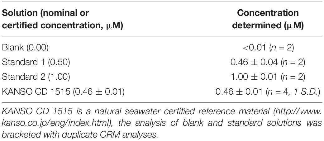
Table 2. The concentration of blank and standard solutions determined by gas-segmented flow techniques upon recovery.

Lab-on-Chip Analytical Cycle

The LoC analyser is a stop flow system whereby reagents and sample/blank/standard are delivered into the absorbance flow cell and then left to react and form colour. All solutions are mixed in a 1:1:1 volume ratio (reagent 1: reagent 2: blank/standard/sample). In this version of the LoC analyser, reagent 1 is added to the sample and these two fluids are mixed, prior to the addition of reagent 2. The flow of the mixed solution is stopped to react for 145 s, and the average reading of the long channel photodiodes during the next 5 s (145–150 s) was used to calculate absorbance (Clinton-Bailey et al., 2017; Grand et al., 2017). The LoC analyser was configured to begin an analytical cycle whenever powered on by the Seaglider. The LoC analyser ran through the following cycle each time it was powered on: (a) Blank, (b) Blank, (c) Standard 1, (d) Standard 2, (e) NaOH wash, (f) Sample, (g) NaOH wash, (h) Sample, (i) NaOH wash, and (j) Sample… until powered off. The first blank was treated as a conditioning sample and was not used in any subsequent computations. This analytical cycle meant that the analyser was calibrated during the downcast of each dive, allowing the upcast to be used for continuous measurements. It took 23 min from the LoC analyser being powered on to the beginning of first sample measurement. Each sample measurement took 8 min. Calibration on each dive allowed compensation for any drift occurring during the deployment.

Raw voltages were converted to absorbance (A) using a modified Beer-Lambert-Bouguer law (Eq. 3; Grand et al., 2017):

$A=-{\text{log}}_{10}(V_{\text{S}}/V_{\text{BLK}}\times I_{\text{BLK}}/I_{\text{S}})(3)$

The second blank (BLK) from each dive was used to calculate the absorbance of standards and samples (S). V_S and V_BLK are the mean voltages from the measurement photodiode of the standard or sample and blank during the 5 s measurement. I_BLK and I_S are the mean voltages of the monitoring photodiodes during this period, which measures LED output during the measurement state of blanks, standards, and samples. Thus I_BLK/I_S is a scaling factor used to correct for drift in LED intensity that may occur from the start of an analytical cycle (blank measurement) to the end (sample measurements).

Seaglider Salinity and Temperature Measurements, Lab-on-Chip Integration and Deployment Details

The LoC PO₄^3– analyser was integrated within the science bay of a Kongsberg Seaglider using an ogive fairing to provide required space. The Seaglider is an autonomous buoyancy driven underwater vehicle capable of deployments down to 1,000 m depth and range and endurance of 4,000 km and several months. Positive Buoyancy is managed by transferring oil from inside the pressure hull to an external bladder, increasing the displacement and causing it to rise though the water column. Removing oil from the bladder has the opposite effect and alternating this pumping cycle produces yo-yo profiling of the glider. Horizontal motion is generated through a combination of body drag and shifting ballast and small wings provide added stability of the platform (Eriksen and Perry, 2009; Meyer, 2016; Rudnick, 2016).

The range of LoC analysers available at NOC use common hardware and software, therefore the physical and electrical integration of the PO₄^3– LoC analyser into the Seaglider followed the procedure described by Vincent et al. (2018), which presents the first LoC glider deployment using a nitrate + nitrite LoC analyser. The sample inlet tube, located on the surface of the payload bay, was fitted with a 0.45 μm poly(ether-sulfone) luer lock syringe filter (MERCK, Millipore, United States). The LoC analyser received power from the Seaglider, and linked via a RS232 serial communication. The Seaglider software uses a CNF file that contains the configuration for each on-board instrument and a CMD file that provides mission parameters. The CNF file enables communication between the Seaglider and the LoC PO₄^3– analyser. The LoC PO₄^3– analyser is set to “logger” mode in the CNF file, which enables the glider to send a number of commands. These commands allow the Seaglider to send and receive data to and from the analyser. Commands include: “clock-set,” used only at the start of each dive, but which enables the analyser to store any time offset between glider and analyser, “status,” which sends the analyser depth every 5 s, and “download,” sent at the end of each dive requesting the sensor to send both ascent and descent data files of processed PO₄^3– values. The sensor transmits only processed data, raw data are accessed upon recovery.

The mission was supported by the MRV Scotia, a Marine Scotland research vessel that managed glider deployment, while conducting a fisheries survey in the northern North Sea, approximately 170 km from the east coast of Scotland (Figure 2A). The Seaglider followed a prescribed south-east to north-west transect approximately 120 km in length, before being piloted to the south-west for recovery. The Seaglider conducted 1,555 dives from 15/08/2018 to 28/09/2018, with 71 dives including PO₄^3– measurements providing 353 individual PO₄^3– measurements. Bidirectional communication between the Seaglider and base station, through an Iridium satellite connection, allowed dive configurations to be modified once deployed and near-real time processed data to be viewed at the base station. The glider operated in two flight modes, “standard” and “loiter” following methods described by Vincent et al. (2018; Figures 2B,C). Standard flight mode adjusts pitch and buoyancy to maintain a uniform glide slope and speed during descent and ascent and was used to transit efficiently between deployment, waypoint and recovery locations. The short duration of profiles in standard flight mode allowed for a maximum of 2 PO₄^3– measurements per dive, and sometimes zero. A loiter flight mode was adopted to lengthen the duration of a dive by reducing the angle of ascent for 30 min following the Seaglider reaching its maximum dive depth. Loiter flight mode was used during high resolution PO₄^3– transects and increased sampling to 6 or 7 PO₄^3– measurements per ascending profile.

FIGURE 2

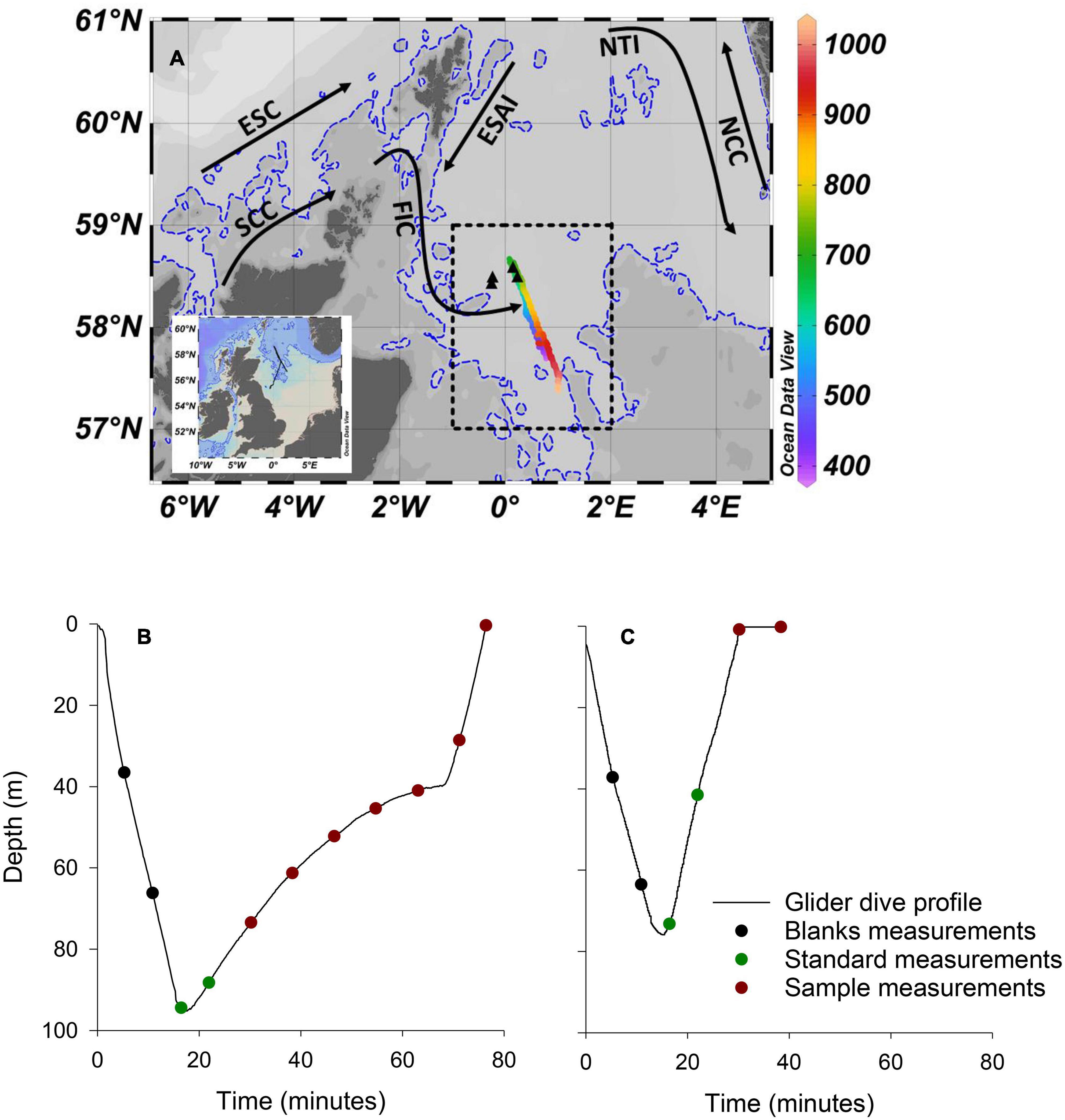
Figure 2. Deployment location and dive profiles. (A) Map of the study area with complete Seaglider track shown on inset map. The colour bar represents the dive number. Dives <379 and >1,034, which included minimal PO₄^3– sampling as the glider was piloted toward deployment and recovery locations, respectively, and are not shown on main figure. Transect 1 included dives numbered 390–690. Transect 2 included dives numbered 691–1,034. The dashed rectangle encompasses the area of the North Sea Biogeochemical Climatology used for comparison (see text for details). Black triangles are the location of 4 RV Heincke sampling stations used for comparison (see text for details). Dashed blue line is the 100 m isobath. Black arrows are approximate paths of the Fair Isle Current (FIC), East Shetland Atlantic Inflow (ESAI), Scottish Coastal Current (SCC), European Slope Current (ESC), Norwegian Trench Inflow (NTI), and Norwegian Coastal Current (NCC). (B) An example of a “loiter” dive profile. (C) An example of a “standard” dive profile.

In addition to PO₄^3–, the Seaglider measured conductivity, temperature (non-pumped Sea-Bird CT Sail, Seabird Electronics) and pressure (Paine Electronics). The CT sail consists of separate (non-ducted) thermistor and conductivity sensor, the latter inside a protective metal housing. Temperature and conductivity data were extracted and processed using the University of East Anglia Glider Toolbox (Queste, 2013) and arithmetic means calculated for 1 m depth bins. Conductivity is dependent on water temperature as well as ionic strength. The conductivity sensor on the CT sail has a thermal lag response issue when passing through strong temperature gradients due to heat stored in sensor materials. Heat dissipation is affected by the water flow rate through the sensor. While loiter flight mode increases LoC sampling, it also produces slow and variable Seaglider ascent speeds (Figure 2B), and subsequently variable flow rates through the conductivity sensor, which makes thermal inertia corrections difficult and, in this instance unresolvable. Consequently, temperature and salinity data were used from descending profiles for analysis.

Lab-on-Chip Data Screening and Comparison With Nearby Ship-Based Measurements and Climatological Data

It is important to understand the quality of any analytical data. For laboratory analyses, this can be achieved routinely by analysing a series of blanks, standards, and certified reference materials. In addition, the analyst is regularly performing quality control by observing the output of the instrument (e.g., peak shapes and baseline shifts). Clearly, the same degree of constant attention cannot be applied to field deployable autonomous measurement technology; therefore, raw data (353 measurements) retrieved from the analyser upon recovery was subject to the following screening procedure.

(1) Identifying and removing data generated from poor LoC analyser calibrations.

(2) Identifying and removing data that are considered extreme (>1 μM) for this study region.

(3) Identifying and removing extreme negative concentrations (<–0.2 μM).

(4) Identifying data that are below the limit of detection (0.04 μM) and replacing them with a value of half the limit of detection (0.02 μM).

Validation here is defined as the assurance that the generated data meets the need of the end user, in this case oceanographers studying marine biogeochemistry. Two approaches are adopted to assess the validity of the dataset: (1) a comparison with 4 depth profiles, that were collected by partners Hereon from RV Heincke on 30th August 2018 nearby our survey area and (2) comparison with the North Sea Biogeochemical Climatology dataset.

Seawater samples were collected on board the RV Heincke using a sampling rosette (Figure 2). Seawater samples were analysed using a gas segmented flow manifold, Seal AA3 (Norderstedt, Germany), combined with a standard spectrophotometric technique (molybdenum blue) (Hydes et al., 2010). The chemistry is almost identical to that used in the LoC analyser, and previous studies have demonstrated that data generated via gas segmented flow analysis is directly comparable to that generated via LoC analysers (Clinton-Bailey et al., 2017; Grand et al., 2017; Birchill et al., 2019a). The limit of detection for gas segmented flow analysis is 0.01 μM in seawater (SEAL-Analytical, 2019). Every year between 2017 and 2019 the SEAL AA3 HR performance was verified through analysis of QUASIMEME reference samples for estuarine and seawater (Aminot et al., 1997). For PO₄^3–, the Seal AA3 consistently reproduced the expected reference values (z-scores < 1).

The results of the LoC analyser were also compared with version 1.1 of the “North Sea Biogeochemical Climatology” (Laane et al., 1996a; Hinrichs et al., 2017a). This is a 0.25° × 0.25° gridded monthly climatologies of biogeochemical parameters, which covers the region from 47 to 65°N and from 15°W to 15°E. It includes observations from 1960 to 2014. Level 2 data was used in this study. Level 2 data is quality-controlled bin-averaged gridded fields and gaps left where data were missing (i.e., level 2 data is not interpolated between grids). For more details see University of Hamburg technical report (Hinrichs et al., 2017b). We selected the region covering 57 to 59°N and 1°W to 2°E (Figure 2), and calculated a mean profile for this region using the depth bins at 0, 5, 10, 15, 20, 25, 30, 35, 42, 50, 62, 78, and 98 m, defined in the climatology for the months of August and September. Mean values were calculated from a minimum and maximum of 16 and 52 data points, respectively.

Results and Discussion

Lab-on-Chip Long Term Performance and Data Screening

The mean voltage output of the photodiode during 5-s measurement periods of the blank, 0.46 and 1.00 μM standard solutions throughout the deployment is displayed in Figure 3. Over the duration of the deployment, a decrease in voltage output was observed, with noticeable step changes. Importantly, these changes occur proportionally across the blank and standard solutions. By converting raw voltages to absorbance values, it is evident that the shifts in photodiode voltage are not associated with shifts in the sensitivity (ΔA/Δc) of the analyser during deployment (Figures 4A–C). Anecdotally, we report that after passing weak cleaning agent (diluted Deacon 90) through the analyser upon recovery, the raw photodiode voltages returned to initial values. Therefore, the decrease in voltage is likely due to staining of the measurement cell. In this instance the decreasing output of the photodiode did not prevent the analyser from making measurements (i.e., there was always sufficient signal from which to measure absorbance). For longer duration deployments this could become an issue. Therefore, the first recommendation we make for future deployments is to include additional NaOH flushes in the analytical procedure to clean the optical cells.

FIGURE 3

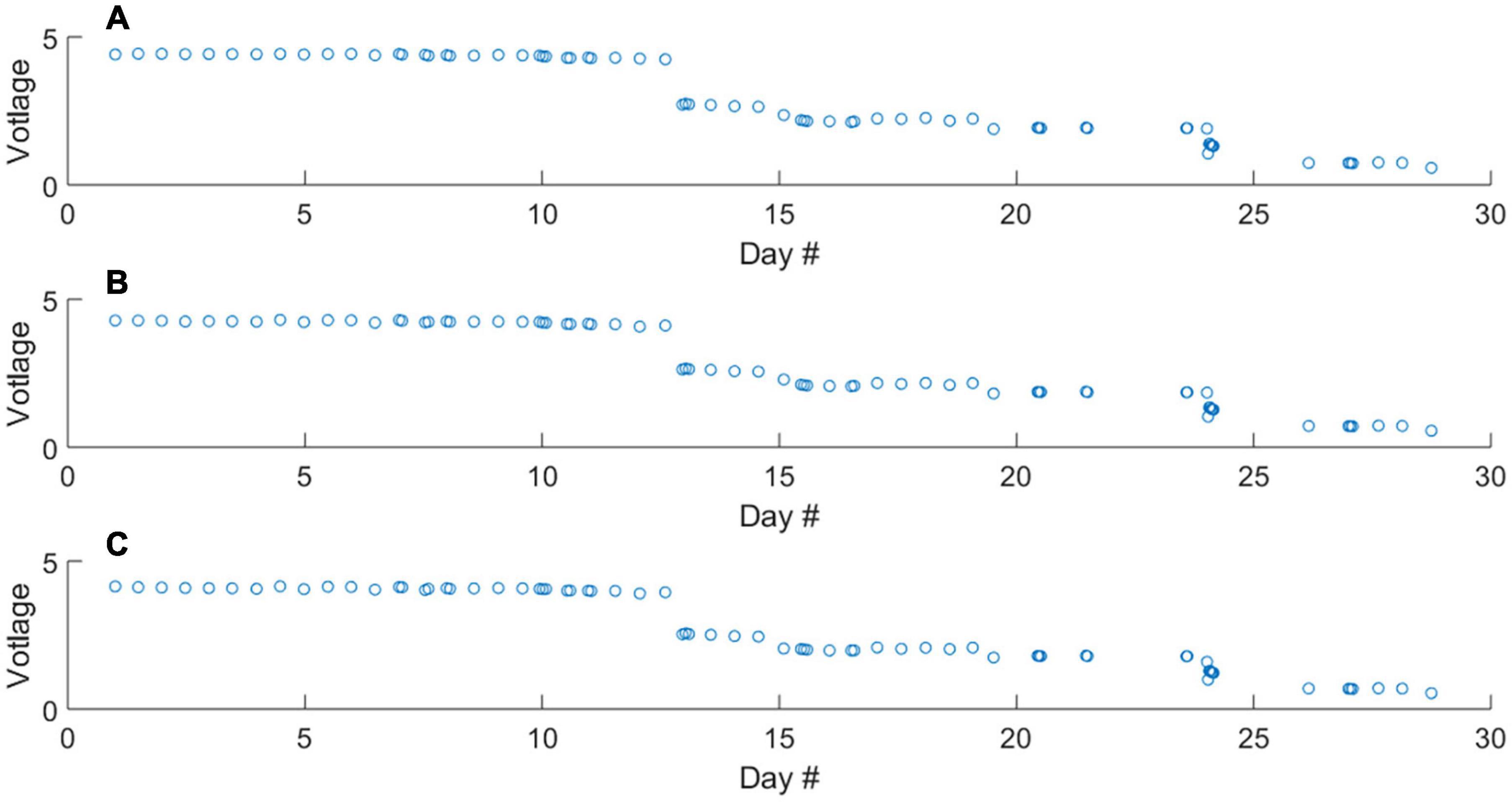
Figure 3. Raw voltage output of the measurement photodiode throughout the deployment during the measurement of the blank (A), 0.46 μM standard (B), and 1.00 μM standard (C) solutions. The differences in raw voltage for respective blank and standard measurements are too small to see, Figure 4 contains absorbance values.

FIGURE 4

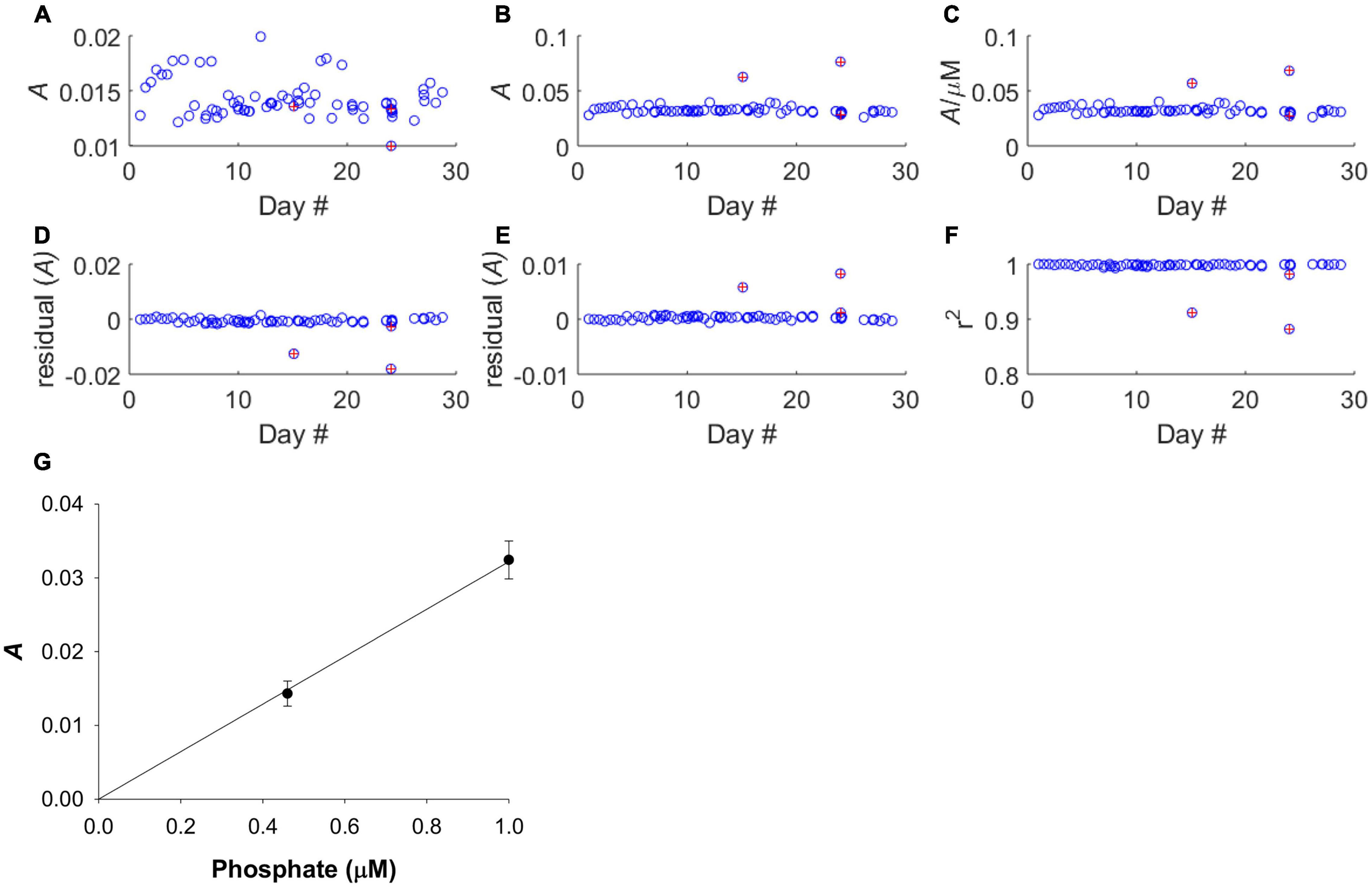
Figure 4. Calibration performance of LoC analyser throughout the deployment. Red markers indicate poor calibrations and data from these dives was removed before further analyses. (A) The absorbance of the 0.46 μM standard. (B) The absorbance of the 1.00 μM standard. (C) Sensitivity of analyser. (D) Residual values for 0.46 μM standard. (E) Residual values for 1.00 μM standard. (F) Correlation co-efficient of regression slope. (G) Average calibration slope for all deployment dives, except those with poor calibrations, with linear fit forced through the zero intercept. The linear fit was based on a mean 0.46 μM PO₄^3– standard absorbance of 0.0143 ± 0.0017, and a mean 1.00 μM PO₄^3– standard absorbance of 0.0324 ± 0.0026. The mean regression slope was 0.0322 ± 0.0027.

The sensitivity of the analyser (ΔA/Δc) showed some variability but no systematic increase or decrease during the course of the deployment (Figures 4A–C), indicating that reagent, blank and standard solutions remained stable under the storage conditions of the deployment, in the dark and at the temperature of the summer North Sea (6–16°C, see Figure 7). A plot of the residual values associated with the linear regression calibration slope exhibited no systematic trend, indicating that a linear regression was appropriate (Figures 4D–G). This is consistent with previous laboratory testing, which demonstrated that the limit of linearity ranged from the limit of quantification to 10 μM (Clinton-Bailey et al., 2017). The calibration procedure required forcing the calibration curve through the origin, because the absorption of both standard points is defined against the “zero” point of the blank. This manipulation resulted in a <1% change in the gradient of the calibration slope. Out of the 71 dives where PO₄^3– was measured, there were three calibrations that were clearly of poor quality (Figures 4D–F). Since only three of 71 calibrations were considered unreliable, containing nine data points, no attempt was made to apply any correction factor (e.g., applying a deployment average calibration slope). Instead, the nine sample data associated with these dives was omitted from the final analyses (Figures 5A,B). A further nine extreme values (>1.0 μM) were removed as likely analytical artefacts (Figure 5C). Although PO₄^3– concentrations in excess of 1 μM are found in North Sea coastal waters (Radach and Pätsch, 1997; Frank et al., 2006), our study location was in the central northern North Sea, where concentrations are typically <1 μM (see validation section below). Moreover, concentrations in excess of 1 μM were distributed randomly suggesting that they resulted from an unidentified source of random error. Similarly, profiles with extreme negative concentrations (<–0.2 μM) were removed from the dataset (six measurements; Figure 5D). In total 24 out 353 measurements, or 7%, were removed from the final dataset before further analysis (Figure 5E).

FIGURE 5

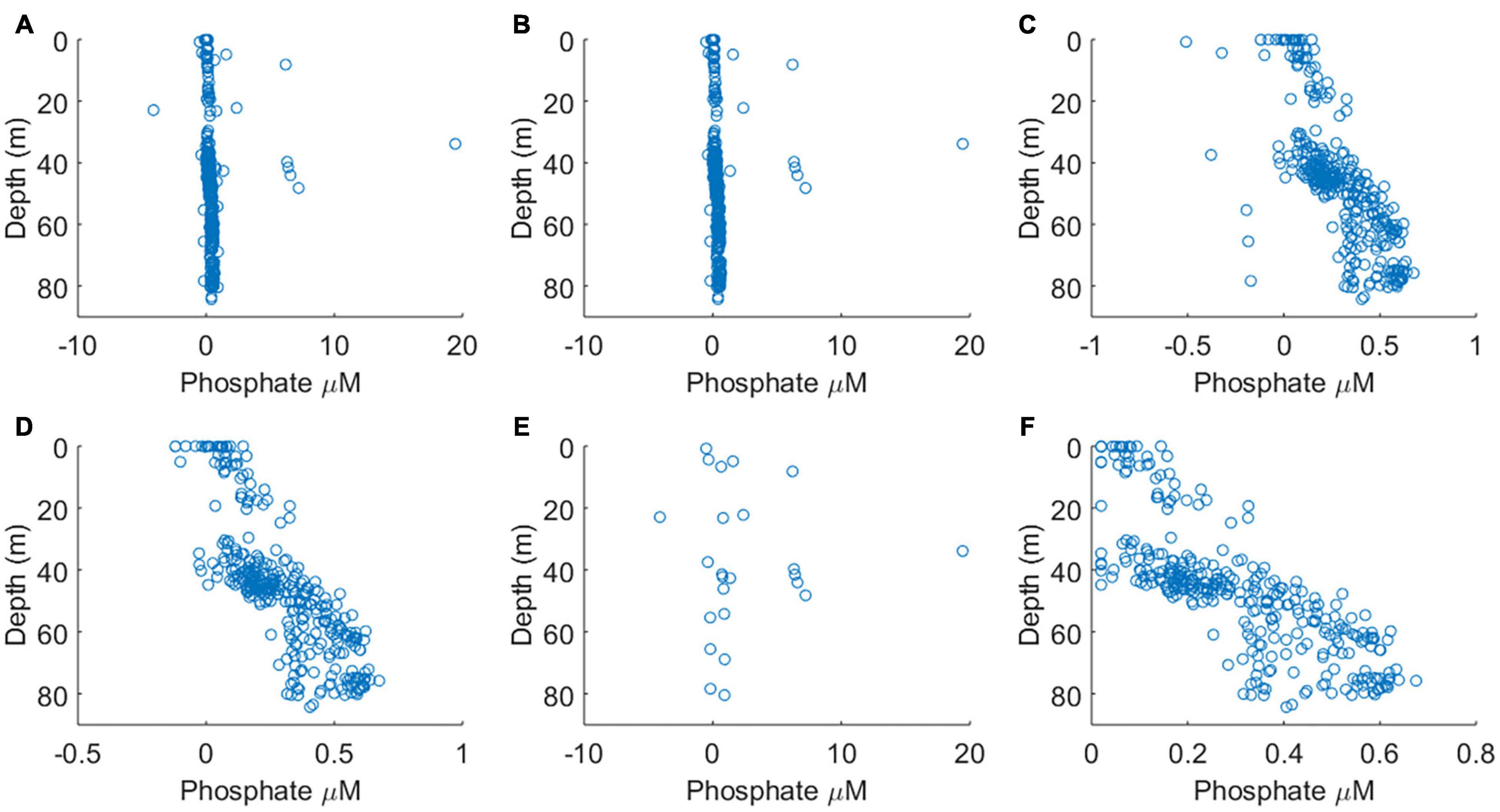
Figure 5. The results of data screening steps carried out, panels (A–D) are in sequence. Note changing horizontal axis scales. (A) The complete dataset. (B) Dataset after the removal of data generated from poor calibrations (see Figure 4). (C) Dataset after the removal of concentrations >1 μM PO₄^3–. (D) Dataset after the removal concentrations <–0.20 μM. (E) All outliers and data resulting from poor calibrations, which were removed from final dataset. (F) The quality controlled data product.

Surface PO₄^3– concentrations were depleted and consequently 68 PO₄^3– measurements were below the limit of quantification (0.14 μM), with 19 of these below the limit of detection (0.04 μM), representing 6% of the dataset. Whilst non-detects do not provide a point measure of PO₄^3– concentration, they do inform us that their PO₄^3– concentration was between 0 and 0.04 μM. The methods available to deal with non-detects include substitution and distribution-based imputation methods, which are recommended when a large proportion of the total observations are non-detects (Baccarelli et al., 2005). Although based on judgment and without statistical basis, substitution methods are simpler and represent a pragmatic approach that is suitable when the proportion of non-detects in the overall dataset is low [e.g., less than 15% (EPA, 2000)]. Consequently, replacing values below the limit of detection with a value equal to half the limit of detection is an approach commonly adopted in studies of environmental chemistry (Vitaliano and Zdanowicz, 1992; Tajimi et al., 2005; García-Fernández et al., 2009). If the scientific outcomes of a study are affected by the treatment of non-detects, the choice of treatment takes on greater importance. Here we simply characterise surface waters as oligotrophic low nutrient environments, therefore the scientific findings are not impacted by the choice of non-detect treatment. Hence, we adopted a simple substitution method. While the oceanographic community is working toward harmonising the use of in situ nutrient sensors, including providing recommendations for defining the limit of detection (Daniel et al., 2020), it is not yet providing recommendations for non-detect treatment. We suggest that treatment of non-detects be clearly defined, particularly when working in oligotrophic waters.

Prior to substitution with LoD/2, some surface values had apparent negative concentrations, as a result of a negative sample absorbance. A negative sample absorbance has no physical meaning and results from a larger voltage generated at the photodiode during the sample measurement than during the blank measurement. A typical cause would be PO₄^3– contamination of the blank solution. However, the blank solution was subsampled upon recovery and found to contain <0.01 μM PO₄^3– (Table 2). Alternatively, it might be caused by sample fluorescence or phosphorescence, or simply be analytical noise resulting from measuring the absorbance of two solutions (blank, low concentration sample) with a small signal.

Comparison With Ship-Based in situ Phosphate Data

To illustrate general trends present in the final data product, the LoC–AUV data was binned into 5 m depth intervals and the arithmetic mean of each depth bin was calculated (Figures 6A,B). The imprint of seasonal stratification is clear within the dataset; low nutrient concentrations characterised surface waters, with a mean PO₄^3– concentration of 0.06 ± 0.04 μM at 0–5 m depth. Between 40 and 60 m depth, there was an increase in the mean concentration of PO₄^3– from 0.17 ± 0.09 to 0.45 ± 0.10 μM, consistent with a seasonal thermocline and remineralisation of sinking organic matter. Below 60 m, the mean PO₄^3– concentration ranged from 0.42 to 0.54 μM. Whilst the imprint of seasonal stratification is clear, the high standard deviation of each depth bin indicate that other processes in addition to seasonal cycling must drive variability.

FIGURE 6

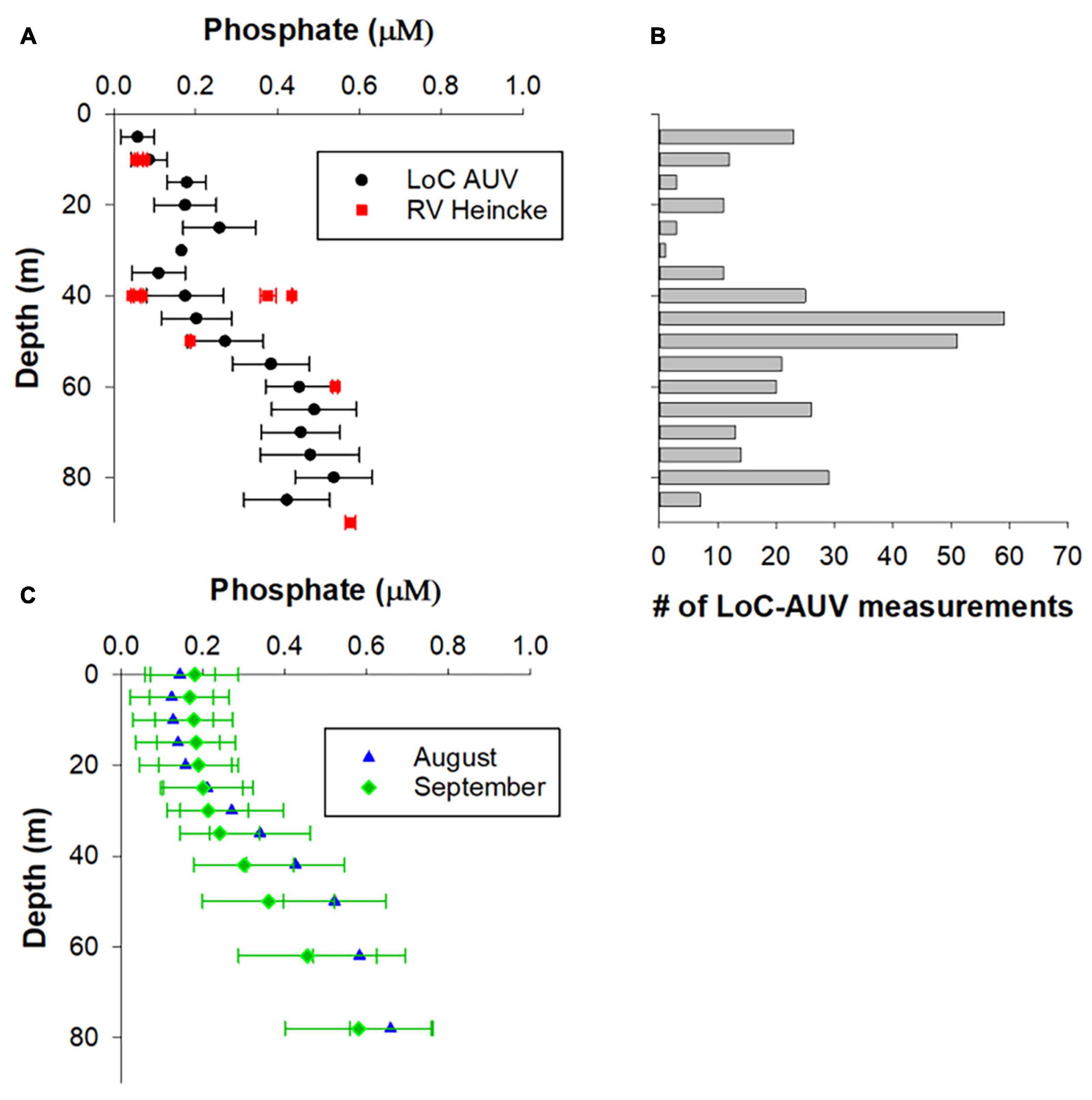
Figure 6. Validation of phosphate LoC–AUV results. (A) LoC–AUV are binned into 5 depth bins and presented as arithmetic mean ± 1 SD. The data from RV Heincke were collected at four locations at the northern end of our transect (see Figure 2 for locations). (B) The number of LoC–AUV measurements within each depth bin. (C) Arithmetic mean ± 1 SD of phosphate concentrations for August and September from the North Sea Biogeochemical Climatology.

The vertical distribution and range of PO₄^3– concentrations determined by LoC–AUV are consistent with traditional shipboard observations made at several depths in the study area on 30th August 30th 2018 (Figure 6A). It is noteworthy that the shipboard observations at 40 m depth were collected at four locations in relatively close proximity (Figure 2), but produced a PO₄^3– concentration range of 0.06–0.44 μM, suggesting large nutrient variability in a relatively small region of the North Sea. Similarly, the mean PO₄^3– concentrations from climatology data for months August and September show surface PO₄^3– depletion in surface waters: 0.11 ± 0.08 μM for August and 0.19 ± 0.12 μM for September, with increasing PO₄^3– concentrations at depth (0.36–0.74 μM, for depth range 42–98 m) (Figure 6C). In agreement with both the LoC–AUV and shipboard observations, the climatology shows considerable variability in PO₄^3– distribution with depth.

In addition to producing accurate and precise PO₄^3– concentrations, LoC–AUV needs to provide oceanographers with spatial and temporal coverage to resolve biogeochemical processes. To provide sufficient resolution to produce a PO₄^3– depth profile, the glider must operate in loiter flight mode (Figure 2). During loiter mode, the reduction in vertical speed of the Seaglider allows for high-resolution measurements through the phosphocline (Figure 6). However, biogeochemical parameters are nearly always interpreted alongside hydrographic data; therefore, it is essential that LoC–AUV provide reliable temperature and salinity measurements. During the upcast of a loiter dive the shallow angle of climb causes slow and variable seawater flow rates through the conductivity cell on the CT sail, thus loiter flight mode is a sub-optimal mode of operation for producing high quality salinity data. Pumped and ducted Conductivity-Temperature-Depth payloads would help mitigate this problem, which have been used on the Seaglider (Janzen and Creed, 2011), and are available on other ocean glider platforms, although the payload requirements for the LoC analyser made the Ogive fairing fitted Seaglider the only viable choice at the time of this study. Increasing the sampling rate of the LoC PO₄^3– analyser would also reduce the need to operate in loiter flight mode. However, the sampling rate is limited by the calibration procedure at the start of each dive, and the reaction rate of the molybdenum blue assay meaning there is a requirement for a 150 s period of colour formation for each blank, standard, and sample measurement.

In situ Measurements of Phosphate in the Northern North Sea

Plots of in situ PO₄^3– concentration, temperature, salinity and density for each transect are presented in Figure 7. There are three primary features evident in the dataset, which are presented and discussed in turn. These are (1) Nutrient depletion in surface waters with enrichment below the seasonal thermocline; (2) The presence of relatively cold, salty bottom layer waters with elevated PO₄^3– concentrations at the northern end of our transect; (3) Horizontally heterogeneous, or “patchy” PO₄^3– distribution.

FIGURE 7

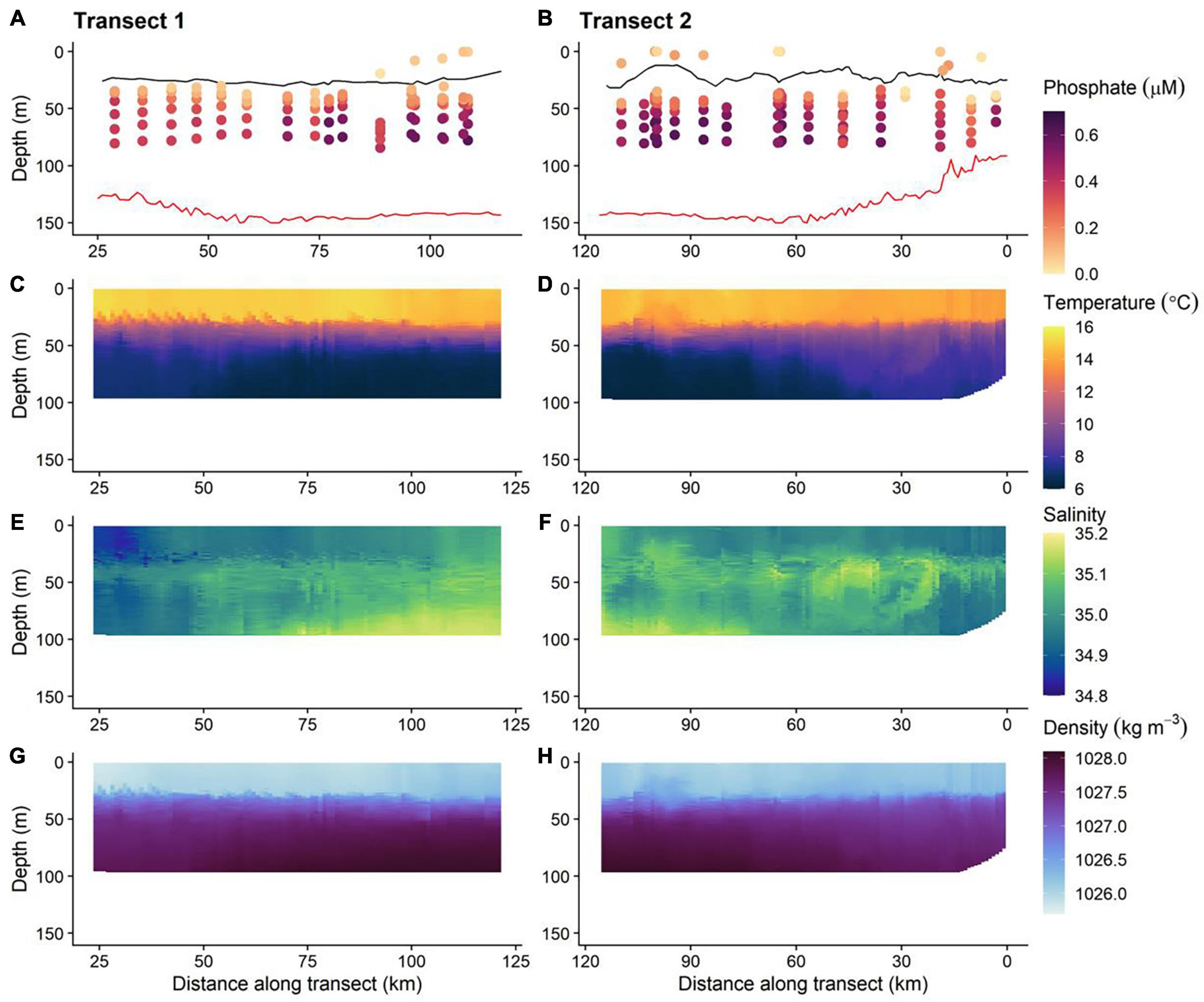
Figure 7. The physical and biogeochemical in situ glider dataset; 0 km is the start transect 1 and the end of transect 2 (i.e., time runs left to right along the horizontal axis). Red and black lines on phosphate plots (A,B) are the GEBCO bathymetry and thermocline, respectively. The location of the thermocline is defined as a 0.03 kg m⁻³ density increase relative to that at 10 m depth (de Boyer Montégut et al., 2004). (C,D) Temperature, (E,F) salinity, and (G,H) density.

The concentration of PO₄^3– was depleted (typically < 0.20 μM) in waters above the seasonal thermocline. PO₄^3– concentrations increased to ≈0.30–0.65 μM in bottom layer waters (Figures 7A,B). The stratification of nutrient concentration corresponds with the location and structure of the thermocline (Figures 7C,D), with low PO₄^3– concentration within warmer surface waters ≈14–16°C and high concentration in bottom layer waters, where temperatures were cold ≈6–9°C. Summer surface nutrient depletion is typical for seasonally stratifying shelf seas, such as the northern North Sea (Painter et al., 2018). This nutrient depletion is a result of uptake by primary producers and export via sinking organic matter during the spring bloom and summer months, coupled with inefficient resupply from nutrient enriched bottom waters due to low levels of vertical mixing across the seasonal thermocline. When estimating the magnitude of seasonal productivity in stratified shelf seas it is important to estimate the diapycnal diffusive flux of nutrients through the thermocline:

$F_{\text{d}}=K_z\frac{\mathrm{\Delta }c}{\mathrm{\Delta }z}(4)$

Where K_z is the eddy diffusivity, Δc is the nutrient concentration gradient through the thermocline, and Δz is the thickness of the thermocline. Shipbased research conducted in the Celtic Sea demonstrated significant variation of the diapycnal nutrient flux (daily mean values of 0.04–2.6 mmol PO₄^3– m^–2 day^–1 with 95% confidence intervals for these mean estimates ranging from 0.00 to 9.0 mmol m^–2 day^–1) (Tweddle et al., 2013). Variability of the diapycnal nutrient flux is driven by the gradient of PO₄^3– through the thermocline, which varied by over an order of magnitude within a 25-h period at a single location, and the variability of K_z, which for example is affected by tidal forces and bathymetry (Sharples et al., 2007; Tweddle et al., 2013). Research ships are ideal for targeted studies, but provide only limited spatial and temporal coverage. Gliders can now be equipped with microstructure turbulence profilers (Palmer et al., 2015) and nutrient analysers (this study; Vincent et al., 2018). Here we demonstrate that LoC–AUV can be used to observe the distribution of PO₄^3– concentrations through the thermocline (Figure 8). Consequently, it is now possible to autonomously collect all the information required to calculate the terms in the vertical diffusive flux equation (Eq. 4) at a greater resolution than shipboard observations. Therefore, autonomous techniques could be used to provide a better constraint of this important rate limiting flux.

FIGURE 8

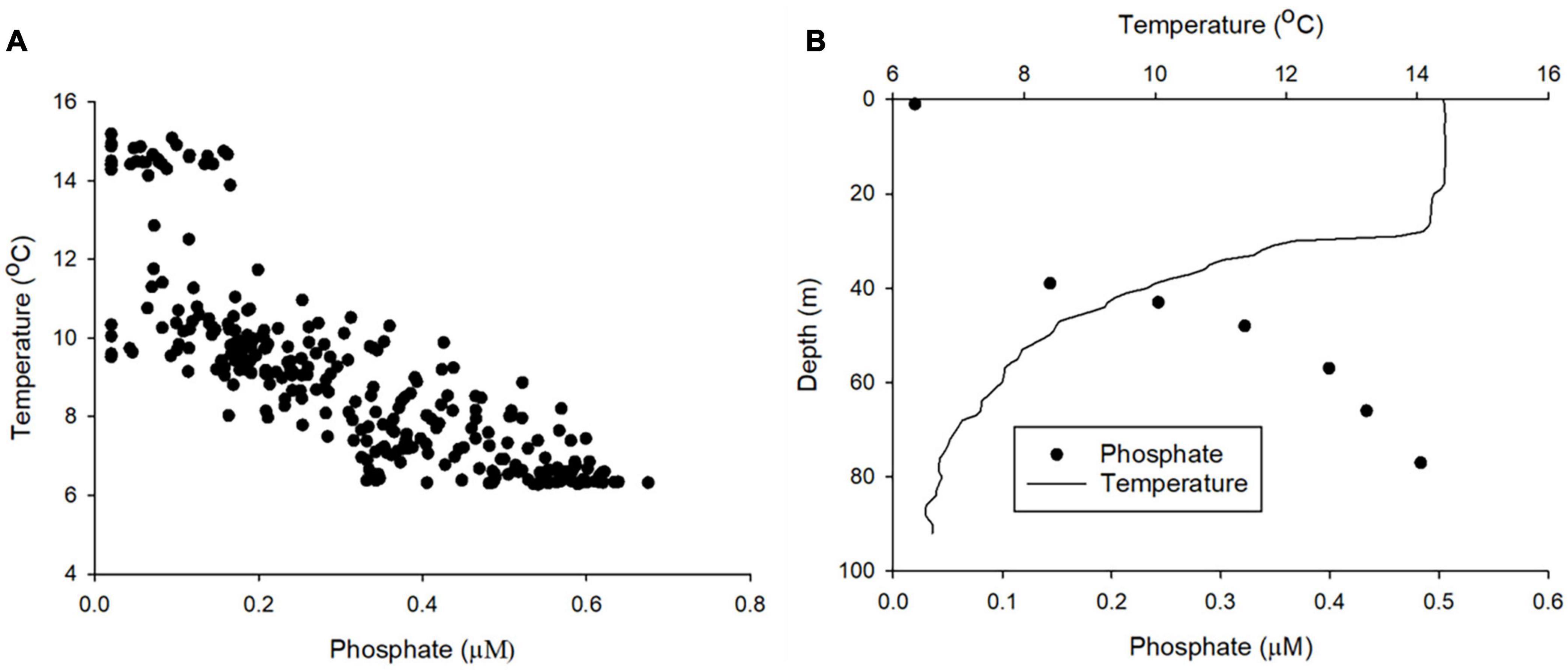
Figure 8. (A) The relationship between phosphate and temperature for the entire dataset. (B) An example depth profile of phosphate and temperature (dive number 883 conducted on 23/08/2018).

Relatively cool, salty bottom layer water found to the northern end of the transect, coincided with the largest observed PO₄^3– concentrations (Figure 7). This suggests that the phosphate-rich deep waters most likely came from the Atlantic Ocean. Inflow from the Atlantic Ocean into the northern North Sea occurs primarily through the Norwegian Trench Inflow (1.2 Sv, 1 Sv = 10⁶ m³ s^–1), Fair Isle Current (FIC; 0.5 Sv) and the East Shetland Atlantic Inflow (ESAF; 0.5 Sv) (Winther and Johannessen, 2006). The Norwegian Trench Inflow largely retroflects with the Norwegian Trench leaving the FIC and ESAF to have the greatest influence on the hydrographic conditions of the northern North Sea (Figure 2). The inflow of Atlantic water via the FIC and ESAF has been shown to be a source of nutrients to the shelf (Laane et al., 1996b; Große et al., 2017), and so natural variability of such transport will lead to an associated variability of inflowing nutrients. Consequently, discrete sampling may not provide a comprehensive representation of seasonal or interannual conditions. Assessment of the current state of shelf sea nutrients is therefore challenging and requires consideration of a range of temporal and spatial scales to suitably capture the temporally and spatially varying drivers that modify observed nutrient data. Observations from AUVs, moorings, shipboard studies and drifters have allowed variability of the physical characteristics of the North Atlantic inflow to the North Sea to be quantified over weekly, seasonal, yearly and decadal timescales (Marsh et al., 2017; Sheehan et al., 2017, 2020; Porter et al., 2018). In contrast, nutrient data are collected at a much coarser resolution via discrete sampling during ship based surveys. Sustained LoC–AUV observations therefore offer the potential to increase the spatial and temporal frequency over which nutrient observations are made and to help extend this physical understanding of shelf seas to include biogeochemical pathways and ecosystem function.

In addition to the general vertical and horizontal trends discussed above, there was noticeable heterogeneity within the PO₄^3– concentrations (Figures 7A,B). This patchiness may be a result of natural variability but may also indicate low levels of precision from the LoC analyser. To evaluate LoC analyser precision, PO₄^3– concentrations were determined during three sequential dives, thereby minimising the effects of natural spatial and temporal variability. Broadly, PO₄^3– concentrations measured at similar depths on sequential dives were within the combined analytical uncertainty determined by laboratory testing (Figure 9A). It is most informative to make direct comparisons at deeper depths where the vertical gradient of PO₄^3– concentration was less steep. Measurements were made at around 75 and 60 m on each of the three dives. The mean PO₄^3– concentrations at the two depths were 0.60 ± 0.01 and 0.53 ± 0.03 μM (1 SD), respectively. Moreover, a significant inverse correlation between temperature and PO₄^3– concentration was observed (Figure 9B), characteristic of seasonally stratified shelf seas (Tweddle et al., 2013). We conclude therefore that the LoC analyser field performance was in line with laboratory testing (u_c = 6.1%), and thus the variation of PO₄^3– concentrations observed in bottom waters (0.30–0.65 μM) was driven by natural variability. Similar variability within macronutrient distributions has been seen in the Hebridean Sea (PO₄^3– concentrations ranging from 0.2 to 0.5 μM within a degree of latitude), and such variability has been identified as an environmental driver of macrophytoplankton distributions (Siemering et al., 2016; Birchill et al., 2019b). In the central northern North Sea, localised patches of elevated summer surface PO₄^3– (>0.5 μM) have been reported by ship based observations (Painter et al., 2018). Repeated observations at two locations in the Celtic Sea showed that the concentration of PO₄^3– in bottom waters ranged from 0.4 to 0.8 μM within a 25-days period (Tweddle et al., 2013). In summary, the patchiness observed in northern North Sea (Figures 7A,B) is characteristic of nutrient distributions in waters overlying the north west European shelf. Shelf seas are dynamic environments impacted by hydrographic and biogeochemical processes occurring over a range of temporal and spatial scales (e.g., phytoplankton blooms, semi diurnal tides and tidal interaction with uneven topography, spring-neap cycles, internal tides, storms, seasonal stratification, and complex regional circulation), which impact phosphorus distributions (Davis et al., 2014; Poulton et al., 2019). When viewed in this context, the observed variability of PO₄^3– concentrations is expected. It is important that future shelf sea deployments of LoC–AUVs are designed with this variability in mind.

FIGURE 9

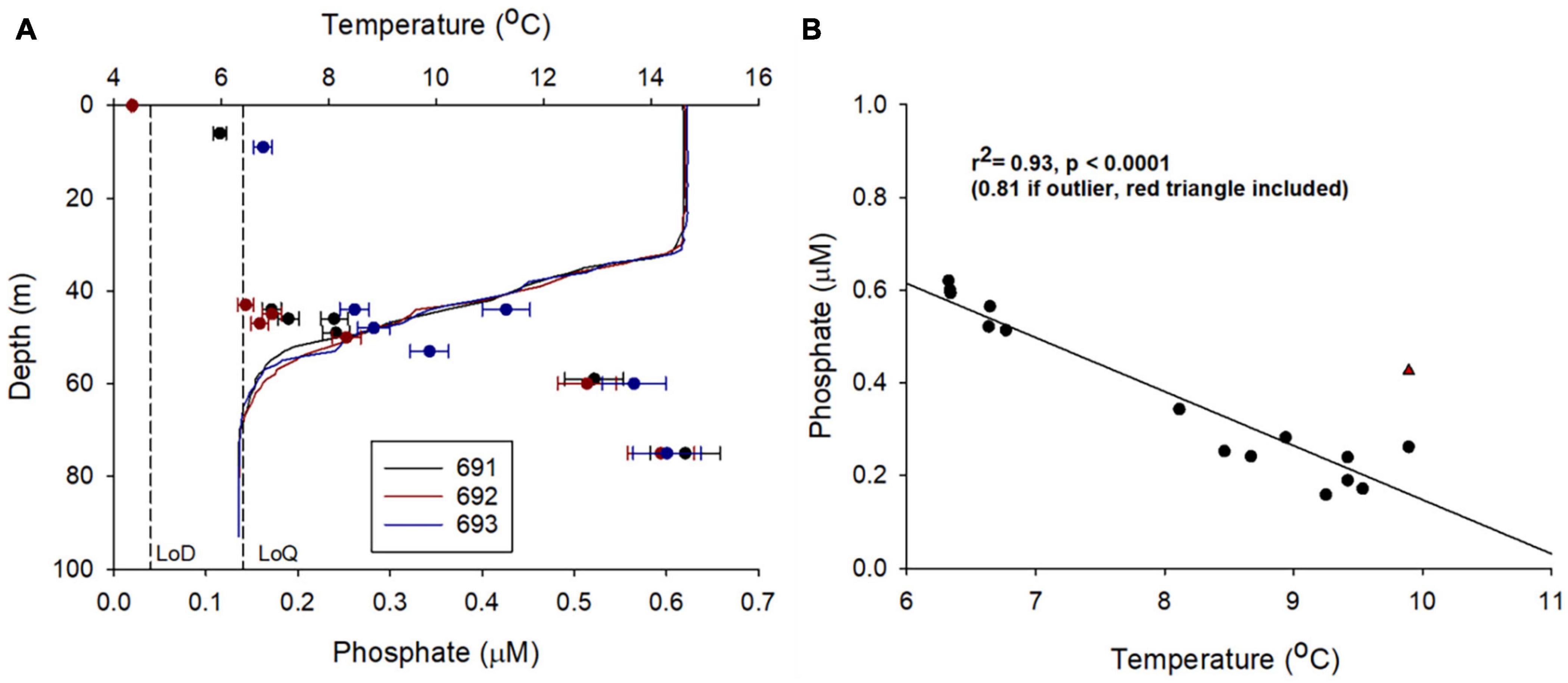
Figure 9. Examining LoC analyser field precision by conducting PO₄^3– analysis during three sequential Seaglider dives (691, 692, and 693), first and last sample separated by 1.98 km and 4.00 h. (A) Depth profiles of temperature and PO₄^3– concentration. Vertical dashed lines are laboratory estimates of the limit of detection (LoD) and limit of quantification (LoQ) (Clinton-Bailey et al., 2017; Grand et al., 2017). Error bars are laboratory estimates of combined (random + systematic) relative uncertainty (Birchill et al., 2019a). (B) Statistically significant inverse linear correlation between temperature and PO₄^3– concentration from dives 691, 692, and 693 for samples collected below 40 m.

Assessing the Extent to Which This Research Has Expanded Glider Sensor Capabilities for Oceanographic Research

The oceanographic research community is experiencing a dramatic increase in capability as autonomous technologies become more accessible (Johnson et al., 2009; Roemmich et al., 2010; Beaton et al., 2012; Heslop et al., 2012; Liblik et al., 2016; Hendry et al., 2019). This study represents the first ever in situ PO₄^3– dataset obtained using an underwater glider and, for that matter, actually any AUV. Therefore, this represents a significant advance in marine biogeochemical capabilities (Jońca et al., 2013). Glider observations are already making an a major contribution to Global Ocean Observing Systems (Testor et al., 2019) and provide a valuable tool to investigate the range of sub-mesoscale phenomena that typify shelf seas and shelf break regions (Roemmich et al., 2010; Liblik et al., 2016). The data presented here provides evidence in support of this assertion, demonstrating the potential of coupling physical and chemical sensors to investigate marine biogeochemical processes. Importantly, an opportunity now exists to combine existing capability to measure NO₃^– and NO₂^– on AUVs (Vincent et al., 2018) with the PO₄^3– LoC–AUV capability demonstrated here. Understanding the controls on nutrient stoichiometry in the ocean has been a central topic of marine research for almost as long as oceanography has existed as a modern scientific discipline, and it remains so to the present day (Redfield, 1934; Moore et al., 2013). It is now a realistic goal to attempt to capture the inorganic N:P stoichiometry of marine systems via simultaneous glider deployments. With current LoC payload requirements this could not happen on a single Seaglider.

In order to put our PO₄^3– LoC–AUV research into the context of wider glider-sensor developments we adopt the Gliders for Research, Ocean Observation and Management (GROOM) approach to sensor development classification (Supplementary Table 1). The GROOM approach utilises two measures of sensor development, Ocean Sciences Technology Readiness Levels (OS-TRL) defined by Waldmann et al. (2010) and Development Status defined by Johnson et al. (2000). To fulfil OS-TRL 3, the sensor must be a commercial product and “Actual systems completed and mission qualified through test and demonstration”. The corresponding Development Status is “III Early stage of development with successful short-term deployments in the marine environment.” We assert that results of the deployment detailed in this manuscript, in combination with recent commercial availability¹, satisfy these requirements and thus PO₄^3– LoC–AUV has fulfilled the requirements of OS-TRL 3 and Development Status II.

LoC–AUV as a Tool for Environmental Management of Regional Seas?

At present, the LoC–AUV technology presented here is used exclusively as a research tool. However, given that now both PO₄^3– and NO₃^– + NO₂^– can be measured by LoC–AUV, and both sensors and platforms are commercially available, it is worth considering the potential applications beyond oceanographic research. Nutrient cycles in coastal waters have been greatly modified by anthropogenic activity. For example riverine phosphorus fluxes have increased 50–300% upon pre-industrial levels (Cordell et al., 2009). Eutrophication of coastal waters can result from anthropogenic nutrient inputs, which can have adverse effects on coastal sea ecosystems such as deoxygenation and increased frequency of harmful algal blooms (Jickells, 1998; Moore et al., 2013; Karl, 2014; Breitburg et al., 2018). Policy at national and international levels has been implemented, which is related, either directly or indirectly, to the issue of eutrophication in the marine environment. The ability to assess the effectiveness of these policies is to a large extent dependent upon sustained observations of inorganic nutrients over timescales of years to decades. As an example, both phosphate and nitrate + nitrite + ammonia are core set indicators (core set indicator 21) used by the European Environment Agency to address policy questions. Current data coverage is geographically biased toward particular regions such as the Baltic Sea, with data coverage in regions such as offshore parts of the Bay of Biscay, Black Sea, and Mediterranean Sea deemed “unsatisfactory” (European-Environment-Agency, 2019). Future ocean observing systems will likely include the capability to autonomously measure macronutrients in the marine environment, and thus will potentially provide data to environmental management agencies with the expanded temporal and spatial resolution they require. The North Sea is an example of an economically important regional sea that is heavily influenced by anthropogenic activity (Emeis et al., 2015), and where various national and international regulation measures are in place (EU, 2008). The nature of this deployment, from a routine fisheries survey, highlights the plausibility that LoC–AUV technology could be readily integrated into existing observing system infrastructure for coastal ocean monitoring.

Recommendations and Conclusion

Recommendations for Further Development

The potential development pathways for new technology are almost infinite, whereas the resources available for this technology development are limited. We therefore take the opportunity to analyse the lessons learned from this and other recent LoC–AUV developments (Vincent et al., 2018) to highlight what we consider important development priorities, besides the ever-present incentive to reduce costs, size, power demand, reagent consumption, and increase sampling frequency.

PO₄^3– LoC–AUV Specific Development Priorities

We consider what criteria remain outstanding in order to fulfil the requirement of OS-TRL 4 (Supplementary Table 1; Actual system proven through successful mission operations and currently operational and available commercially available). A critical step in assessing sensor (or microfluidic analyser) performance is independent validation of in situ results (Waldmann et al., 2010). In this study, we achieve a semi-quantitative validation using data generated from traditional measurement approaches, collected nearby in space and time, and by using a North Sea climatological dataset. Whilst this is sufficient to conclude that we have generated an oceanographically consistent dataset, it does not allow for a robust quantitative validation of the in situ dataset, such as that achieved by Vincent et al. (2018) when deploying a NO₃^– + NO₂^– LoC analyser on a Seaglider in the Celtic Sea. Throughout the field campaign reported by Vincent et al. (2018), water samples were collected using traditional water sampler techniques, followed by traditional benchtop spectrophotometric analysis, allowing for a direct comparison with LoC–AUV data. In order to progress to OS-TRL 4, long-term PO₄^3– LoC–AUV deployments with robust validation are a development priority. Given typical glider speeds (≈25 cm s^–1) and deployment lengths (months) and spatial scales (100–1,000 s km), simultaneous or sequential LoC–AUV deployments may be required to obtain the resolution suitable to study oceanographic processes. To be considered “mission proved,” multiple long-term (>1 month; Supplementary Table 1) deployments that produce valid datasets are required. Glider missions are typically used in conjunction with other measurement platforms (e.g., satellites, research vessels, moored platforms) (Roemmich et al., 2010; Liblik et al., 2016). For unequivocal proof of mission readiness, future PO₄^3– LoC–AUV deployments should be placed within the context of a novel oceanographic observing network (i.e., coordinated to target an oceanographic process) (Hendry et al., 2019).

Expansion of LoC–AUV Parameter Capability

Currently, LoC analysers are available to measure NO₃^– + NO₂^– (Vincent et al., 2018) and PO₄^3– using a LoC–AUV approach. A strength of the LoC technology is that standard hardware and software is used across the range of analysers in development. At NOC these include silicic acid, pH, dissolved inorganic carbon, total alkalinity, ammonia and iron. As the future LoC analyser technology matures, physical and electrical integration with autonomous platforms, such as the Seaglider used in this study, can follow already established procedures (this study; Vincent et al., 2018). Being able to collect concurrent measurements of multiple important chemical parameters will expand research horizons. Ideally, size and power requirements would permit this to occur on a single platform, presently larger AUV platforms should be considered or objectives may be met using multiple simultaneous AUV deployments.

Expansion of Platform Integration

There are multiple autonomous platforms available, which each offer different advantages and disadvantages. There are different types of glider (e.g., Seaglider, Slocum, and Spray) available, whose merits have been reviewed in detail elsewhere (Meyer, 2016; Rudnick, 2016). Some differences pertinent to LoC integration are highlighted here. The Slocum Electric’s buoyancy engine and tail fin rudder give it a tight turning circle (7 m), making it well suited to shallow water (30–200 m) operations, such as the deployments presented here and by Vincent et al. (2018). Additionally, an optional propulsion system means it can generate horizontal as well as vertical motion, allowing it to pass through strong pycnoclines and currents, common in shelf seas. However, the payload requirements of the LoC analyser restricts internal housing of the sensor to the Ogive modified Seaglider for ocean glider deployments at the time of writing. Further NOC developments are currently being trialled with a Slocum glider that will enable external housing of the LoC analyser, which would expand the range of platforms suitable for integration.

Deep ocean exploration typically uses a range of larger AUVs (e.g., WHOI’s Sentry and the NOC Autosub). Integration of LoC analysers onto such platforms offers the opportunity to extend biogeochemical capability to deep ocean environments enabling, for instance, monitoring impacts of deep-sea mining or investigating the influence of hydrothermal exchange on deep ocean biogeochemistry. Autosub offers the possibility to house up to 9 LoC analysers simultaneously and research is ongoing to integrate LoC analysers into Autosub (A. Schaap, personal communication, August 2020). For the PO₄^3– LoC analyser specifically, the current minimum operating temperature of 5°C (Table 1) would limit deep ocean observations. Integration into an ever-expanding fleet of autonomous surface vehicles would offer an opportunity to study the surface ocean in detail, where primary production and air-sea gas exchange occurs.

Conclusion

We report the integration of a PO₄^3– LoC analyser into a Seaglider, successfully deployed in the northern North Sea for a period of 44 days to measure PO₄^3– concentrations along a 120 km transect (surveyed twice). Validation of in situ data was achieved through comparison with nearby ship board measurements and climatology data, demonstrating our ability to produce high quality, oceanographically consistent, in situ measurements. As the first demonstration of in situ PO₄^3– measurements using an AUV, this study represents a step forward in glider-sensor capabilities opening up new research horizons. More broadly, LoC–AUV offers the exciting possibility to autonomously observe a range of important chemical parameters in situ and can make important contributions to the global effort to leave the era of ocean data scarcity behind. Thus, LoC–AUV should be considered in the design of future ocean observing systems.

Data Availability Statement

The datasets presented in this study can be found in online repositories. The names of the repository/repositories and accession number(s) can be found below: British Oceanographic Data Centre, doi: 10.5285/bf632e43-d8e9-43ab-e053-6c86abc0ab7a.

Ethics Statement

Written informed consent was obtained from the individual(s) for the publication of any potentially identifiable images or data included in this article.

Author Contributions

MP, ADB, AJB, AS, RP, MM, CW, TH, and JK contributed to the conception and design of the study. AJB, processed Lab-on-Chip data and wrote the first draft of the manuscript. TH processed CT sail data. YV provided macronutrient analysis. All co-authors contributed to the manuscript revision and approved the submitted version.

Funding

This research was funded by the National Environment Research Council AlterEco Grant (Grant No. NE/P013899/1). This provided funding for the bulk of the work-deployment of seaglider and fabrication and testing of lab-on-chip analyser. Funding for Heincke cruise was awarded to Rüdiger Röttgers and Holger Brix (Hereon), for project ShelfVal. Hereon funding was provided by the Helmholtz Association PACES II Program: Polar regions and coasts in the changing earth system.

Conflict of Interest

MM, ADB, and RP are co-founders and employees of Clearwater Sensors.

The remaining authors declare that the research was conducted in the absence of any commercial or financial relationships that could be construed as a potential conflict of interest.

Acknowledgments

We thank the captain and crew of MRV Scotia and the RV Heincke. We thank John Walk (Ocean Technology and Engineering, National Oceanography Centre), Michael Smart and Steven Woodward (Marine Autonomous Robotic Systems, National Oceanography Centre) for their invaluable input during LoC analyser Seaglider integration and deploying, piloting and recovering the Seaglider. We also thank Christian Ahlers, Alina Zacharzewski, and Tanja Pieplow (Helmholtz-Zentrum Hereon) for helping to collect and analyze discrete nutrient samples.

Supplementary Material

The Supplementary Material for this article can be found online at: https://www.frontiersin.org/articles/10.3389/fmars.2021.698102/full#supplementary-material

Footnotes

1. ^ http://www.clearwatersensors.com/

References

Adornato, L. R., Kaltenbacher, E. A., Greenhow, D. R., and Byrne, R. H. (2007). High-resolution in situ analysis of nitrate and phosphate in the oligotrophic ocean. Environ. Sc. Technol. 41, 4045–4052. doi: 10.1021/es0700855

PubMed Abstract | CrossRef Full Text | Google Scholar

Aminot, A., and Kérouel, R. (1997). Assessment of heat treatment for nutrient preservation in seawater samples. Anal. Chim. Acta 351, 299–309. doi: 10.1016/S0003-2670(97)00366-8

CrossRef Full Text | Google Scholar

Aminot, A., Kirkwood, D., and Carlberg, S. (1997). The QUASIMEME laboratory performance studies (1993–1995): overview of the nutrients section. Mari. Pollut. Bull. 35, 28–41. doi: 10.1016/S0025-326X(97)80876-4

CrossRef Full Text | Google Scholar

Baccarelli, A., Pfeiffer, R., Consonni, D., Pesatori, A. C., Bonzini, M., Patterson, D. G., et al. (2005). Handling of dioxin measurement data in the presence of non-detectable values: overview of available methods and their application in the Seveso chloracne study. Chemosphere 60, 898–906. doi: 10.1016/j.chemosphere.2005.01.055

PubMed Abstract | CrossRef Full Text | Google Scholar

Barus, C., Romanytsia, I., Striebig, N., and Garçon, V. (2016). Toward an in situ phosphate sensor in seawater using Square Wave Voltammetry. Talanta 160, 417–424. doi: 10.1016/j.talanta.2016.07.057

PubMed Abstract | CrossRef Full Text | Google Scholar

Beaton, A. D., Cardwell, C. L., Thomas, R. S., Sieben, V. J., Legiret, F.-E., Waugh, E. M., et al. (2012). Lab-on-chip measurement of nitrate and nitrite for in situ analysis of natural waters. Environ. Sci. Technol. 46, 9548–9556.

Google Scholar

Beaton, A. D., Sieben, V. J., Floquet, C. F., Waugh, E. M., Bey, S. A. K. I, Ogilvie, R., et al. (2011). An automated microfluidic colourimetric sensor applied in situ to determine nitrite concentration. Sensors Actuat. B Chem. 156, 1009–1014.

Google Scholar

Birchill, A. J., Clinton-Bailey, G., Hanz, R., Mawji, E., Cariou, T., White, C., et al. (2019a). Realistic measurement uncertainties for marine macronutrient measurements conducted using gas segmented flow and Lab-on-Chip techniques. Talanta 200, 228–235.

Google Scholar

Birchill, A. J., Hartner, N., Kunde, K., Siemering, B., Daniels, C., Gonzalez-Santana, D., et al. (2019b). The eastern extent of seasonal iron limitation in the high latitude North Atlantic Ocean. Sci. Rep. 9, 1–12.

Google Scholar

Breitburg, D., Levin, L. A., Oschlies, A., Grégoire, M., Chavez, F. P., Conley, D. J., et al. (2018). Declining oxygen in the global ocean and coastal waters. Science 359:eaam7240. doi: 10.1126/science.aam7240

PubMed Abstract | CrossRef Full Text | Google Scholar

Burton, J. D. (1973). Problems in the analysis of phosphorus compounds. Water Res. 7, 291–307. doi: 10.1016/0043-1354(73)90170-X

CrossRef Full Text | Google Scholar

Cleary, J., Maher, D., Slater, C., and Diamond, D. (2010). “In situ monitoring of environmental water quality using an autonomous microfluidic sensor,” in Proceeding Ofpaper Presented at 2010 IEEE Sensors Applications Symposium (SAS), 23–25.

Google Scholar

Clementson, L. A., and Wayte, S. E. (1992). The effect of frozen storage of open-ocean seawater samples on the concentration of dissolved phosphate and nitrate. Water Res. 26, 1171–1176. doi: 10.1016/0043-1354(92)90177-6

PubMed Abstract | CrossRef Full Text | Google Scholar

Clinton-Bailey, G. S., Grand, M. M., Beaton, A. D., Nightingale, A. M., Owsianka, D. R., Slavik, G. J., et al. (2017). A lab-on-chip analyzer for in situ measurement of soluble reactive phosphate: improved phosphate blue assay and application to fluvial monitoring. Environ. Sci. Technol. 51, 9989–9995. doi: 10.1021/acs.est.7b01581

PubMed Abstract | CrossRef Full Text | Google Scholar

Cohen, M. J., Kurz, M. J., Heffernan, J. B., Martin, J. B., Douglass, R. L., Foster, C. R., et al. (2013). Diel phosphorus variation and the stoichiometry of ecosystem metabolism in a large spring-fed river. Ecol. Monog. 83, 155–176. doi: 10.1890/12-1497.1

CrossRef Full Text | Google Scholar

Cordell, D., Drangert, J.-O., and White, S. (2009). The story of phosphorus: global food security and food for thought. Global Environ. Change 19, 292–305. doi: 10.1016/j.gloenvcha.2008.10.009

CrossRef Full Text | Google Scholar

Daniel, A., Laës-Huon, A., Barus, C., Beaton, A. D., Blandfort, D., Guigues, N., et al. (2020). Toward a harmonization for using in situ nutrient sensors in the marine environment. Front. Mari. Sci. 6:773. doi: 10.3389/fmars.2019.00773

CrossRef Full Text | Google Scholar

Davis, C. E., Mahaffey, C., Wolff, G. A., and Sharples, J. (2014). A storm in a shelf sea: Variation in phosphorus distribution and organic matter stoichiometry. Geophys. Res. Lett. 41, 8452–8459. doi: 10.1002/2014GL061949

CrossRef Full Text | Google Scholar

de Boyer Montégut, C., Madec, G., Fischer, A. S., Lazar, A., and Iudicone, D. (2004). Mixed layer depth over the global ocean: an examination of profile data and a profile-based climatology. J. Geophys. Res. Oceans 109:C12003. doi: 10.1029/2004JC002378

CrossRef Full Text | Google Scholar

Dore, J. E., Houlihan, T., Hebel, D. V., Tien, G., Tupas, L., and Karl, D. M. (1996). Freezing as a method of sample preservation for the analysis of dissolved inorganic nutrients in seawater. Mari. Chem. 53, 173–185. doi: 10.1016/0304-4203(96)00004-7

CrossRef Full Text | Google Scholar

Emeis, K.-C., van Beusekom, J. E. E., Callies, U., Ebinghaus, R., Kannen, A., Kraus, G., et al. (2015). The north seaa shelf sea in the anthropocene. J. Mari. Syst. 141, 18–33. doi: 10.1016/j.jmarsys.2014.03.012

CrossRef Full Text | Google Scholar

EPA (2000). Guidance for Data Quality Assessment Practical Methods for Data Analysis EPA QA/G-9Rep., Office of Environmental Information. Washington DC: USA.

Google Scholar

Eriksen, C. C., and Perry, M. J. (2009). The nurturing of seagliders by the national oceanographic partnership program. Oceanography 22, 146–157. doi: 10.5670/oceanog.2009.45

CrossRef Full Text | Google Scholar

EU (2008). Directive 2008/56/EC of the european parliament and of the council. Offi. J. Eur. Union.

Google Scholar

European-Environment-Agency (2019). Nutrient Enrichment and Eutrophication in Europe’s Seas: Moving Towards A Healthy Marine Environmentrep. Luxembourg: European Union.

Google Scholar

Frank, C., Schroeder, F., Ebinghaus, R., and Ruck, W. (2006). Using sequential injection analysis for fast determination of phosphate in coastal waters. Talanta 70, 513–517. doi: 10.1016/j.talanta.2005.12.055

PubMed Abstract | CrossRef Full Text | Google Scholar

García-Fernández, A. J., Gómez-Ramírez, P., Martínez-López, E., Hernández-García, A., María-Mojica, P., Romero, D., et al. (2009). Heavy metals in tissues from loggerhead turtles (Caretta caretta) from the southwestern Mediterranean (Spain). Ecotoxicol. Environ. Safety 72, 557–563. doi: 10.1016/j.ecoenv.2008.05.003

PubMed Abstract | CrossRef Full Text | Google Scholar

Gardolinski, P. C., Hanrahan, G., Achterberg, E. P., Gledhill, M., Tappin, A. D., House, W. A., et al. (2001). Comparison of sample storage protocols for the determination of nutrients in natural waters. Water Res. 35, 3670–3678. doi: 10.1016/S0043-1354(01)00088-4

CrossRef Full Text | Google Scholar

Gilbert, M., Needoba, J., Koch, C., Barnard, A., and Baptista, A. (2013). Nutrient loading and transformations in the columbia river estuary determined by high-resolution in situ sensors. Estuar. Coasts 36, 708–727. doi: 10.1007/s12237-013-9597-0

CrossRef Full Text | Google Scholar

Grand, M. M., Clinton-Bailey, G. S., Beaton, A. D., Schaap, A. M., Johengen, T. H., Tamburri, M. N., et al. (2017). A lab-on-chip phosphate analyzer for long-term in situ monitoring at fixed observatories: optimization and performance evaluation in estuarine and oligotrophic coastal waters. Front. Mari. Sci. 4:255. doi: 10.3389/fmars.2017.00255

CrossRef Full Text | Google Scholar

Große, F., Kreus, M., Lenhart, H.-J., Pätsch, J., and Pohlmann, T. (2017). A novel modeling approach to quantify the influence of nitrogen inputs on the oxygen dynamics of the North Sea. Front. Mari. Sci. 4:383. doi: 10.3389/fmars.2017.00383

CrossRef Full Text | Google Scholar

Hendry, K. R., Huvenne, V. A. I., Robinson, L. F., Annett, A., Badger, M., Jacobe, A. W., et al. (2019). The biogeochemical impact of glacial meltwater from southwest greenland. Prog. Oceanog. 176:102126. doi: 10.1016/j.pocean.2019.102126

CrossRef Full Text | Google Scholar

Heslop, E. E., Ruiz, S., Allen, J., ópez-Jurado, J. L. L., Renault, L., and Tintoré, J. (2012). Autonomous underwater gliders monitoring variability at “choke points” in our ocean system: a case study in the Western Mediterranean Sea. Geophys. Res. Lett. 39:L20604. doi: 10.1029/2012gl053717

CrossRef Full Text | Google Scholar

Hinrichs, I., Gouretski, V., Pätsch, J., Emeis, K., and Stammer, D. (2017b). North Sea Biogeochemical Climatology Technical ReportRep. Germany: CEN (Center for Earth System Research and Sustainability).

Google Scholar

Hinrichs, I., Gouretski, V., Pätsch, J., Emeis, K.-C., and Stammer, D. (2017a). North Sea Biogeochemical Climatology (Version 1.0). Hamburg, World Data Center for Climate (WDCC) at DKRZ, doi: 10.1594/WDCC/NSBClim_v1.0.

CrossRef Full Text | Google Scholar

Hydes, D., Aoyama, M., Aminot, A., Bakker, K., Becker, S., Coverly, S., et al. (2010). “Determination of dissolved nutrients (N, P, SI) in seawater with high precision and inter-comparability using gas-segmented continuous flow analysers,” in The GO-SHIP Repeat Hydrography Manual: A Collection of Expert Reports and Guidelines. Version 1. IOCCP Report Number 14, ICPO Publication Series Number 134, eds E. M. Hood, C. L. Sabine, and B. M. Sloyan, doi: 10.25607/OBP-15, Available online at: http://www.go-ship.org/HydroMan.html

CrossRef Full Text | Google Scholar

HydroMet, O. (2020). Technical Data Sea-Bird Scientific HydroCycle-PO4 Phosphate Sensor. OTT. Available online at: https://www.ott.com/en-uk/products/water-quality-2/sea-bird-scientific-hydrocycle-po4-phosphate-sensor-1528/productAction/outputAsPdf/ (accessed April 2020).

Google Scholar

Janzen, C. D., and Creed, E. L. (2011). “Physical oceanographic data from Seaglider trials in stratified coastal waters using a new pumped payload CTD,” in Proceeding of the Paper Presented at OCEANS’11 MTS/IEEE KONA 19–22.

Google Scholar

Jickells, T. (1998). Nutrient biogeochemistry of the coastal zone. Science 281, 217–222. doi: 10.1126/science.281.5374.217

PubMed Abstract | CrossRef Full Text | Google Scholar

Johnson, K., Byrne, B., Balch, B., Bender, M., Benner, R., Bishop, J., et al. (2000). Modern observing sytems working group summary. New York: NY, OCTET.

Google Scholar

Johnson, K. S., Berelson, W. M., Boss, E. S., Chase, Z., Claustre, H., Emerson, S. R., et al. (2009). Observing biogeochemical cycles at global scales with profiling floats and gliders: prospects for a global array. Oceanography 22, 216–225. doi: 10.5670/oceanog.2009.81

CrossRef Full Text | Google Scholar

Jońca, J., Comtat, M., and Garçon, V. (2013). “Smart sensors for real-time water quality monitoring. smart sensors,” in Measurement and Instrumentation, eds S. C. Mukhopadhyay and A. Mason (Berlin: Springer), doi: 10.1007/978-3-642-37006-9_2

CrossRef Full Text | Google Scholar

Jońca, J., León Fernández, V., Thouron, D., Paulmier, A., Graco, M., and Garçon, V. (2011). Phosphate determination in seawater: toward an autonomous electrochemical method. Talanta 87, 161–167. doi: 10.1016/j.talanta.2011.09.056

PubMed Abstract | CrossRef Full Text | Google Scholar

Karl, D. M. (2014). Microbially mediated transformations of phosphorus in the sea: new views of an old cycle. Ann. Rev. Mari. Sci. 6, 279–337. doi: 10.1146/annurev-marine-010213-135046

PubMed Abstract | CrossRef Full Text | Google Scholar

Kattner, G. (1999). Storage of dissolved inorganic nutrients in seawater: poisoning with mercuric chloride. Mari. Chem. 67, 61–66. doi: 10.1016/S0304-4203(99)00049-3

CrossRef Full Text | Google Scholar

Laane, R., van Leussen, W., Radach, G., Berlamont, J., Sündermann, J., van Raaphorst, W., et al. (1996a). North-west European shelf programme (NOWESP): an overview. Deutsche Hydrografische Zeitschrift 48, 217–229.

Google Scholar

Laane, R. W., Svendsen, E., Radach, G., Groeneveld, G., Damm, P., PÄtsch, J., et al. (1996b). Variability in fluxes of nutrients (N, P, Si) into the North Sea from the atlantic ocean and skagerrak caused by variability in water flow. Deutsche Hydrografische Zeitschrift 48, 401–419.

Google Scholar

Legiret, F.-E., Sieben, V. J., Woodward, E. M. S., Abi Kaed Bey, S. K., Mowlem, M. C., Connelly, D. P., et al. (2013). A high performance microfluidic analyser for phosphate measurements in marine waters using the vanadomolybdate method. Talanta 116, 382–387. doi: 10.1016/j.talanta.2013.05.004

PubMed Abstract | CrossRef Full Text | Google Scholar

Liblik, T., Karstensen, J., Testor, P., Alenius, P., Hayes, D., Ruiz, S., et al. (2016). Potential for an underwater glider component as part of the global ocean observing system. Methods Oceanog. 17, 50–82. doi: 10.1016/j.mio.2016.05.001

CrossRef Full Text | Google Scholar

Lyddy-Meaney, A. J., Ellis, P. S., Worsfold, P. J., Butler, E. C., and McKelvie, I. D. (2002). A compact flow injection analysis system for surface mapping of phosphate in marine waters. Talanta 58, 1043–1053. doi: 10.1016/S0039-9140(02)00428-9

CrossRef Full Text | Google Scholar

Marsh, R. I, Haigh, D., Cunningham, S. A., Inall, M. E., Porter, M., and Moat, B. I. (2017). Large-scale forcing of the European slope current and associated inflows to the north sea. Ocean Sci. 13, 315–335. doi: 10.5194/os-13-315-2017

CrossRef Full Text | Google Scholar

Meyer, D. (2016). Glider technology for ocean observations: a review. Ocean Sci. Dis. 2016, 1–26.

Google Scholar

Moore, C., Mills, M., Arrigo, K., Berman-Frank, I., Bopp, L., Boyd, P., et al. (2013). Processes and patterns of oceanic nutrient limitation. Nat. Geosci. 6, 701–710. doi: 10.1038/ngeo1765

CrossRef Full Text | Google Scholar

Murphy, J., and Riley, J. P. (1962). A modified single solution method for the determination of phosphate in natural waters. Anal. Chim. Acta 27, 31–36. doi: 10.1016/S0003-2670(00)88444-5

CrossRef Full Text | Google Scholar

Nagul, E. A. I, McKelvie, D., Worsfold, P., and Kolev, S. D. (2015). The molybdenum blue reaction for the determination of orthophosphate revisited: opening the black box. Anal. Chim. Acta 890, 60–82. doi: 10.1016/j.aca.2015.07.030

PubMed Abstract | CrossRef Full Text | Google Scholar

Nightingale, A. M., Beaton, A. D., and Mowlem, M. C. (2015). Trends in microfluidic systems for in situ chemical analysis of natural waters. Sensors Actuat. B Chem. 221, 1398–1405. doi: 10.1016/j.snb.2015.07.091

CrossRef Full Text | Google Scholar

Painter, S. C., Lapworth, D. J., Woodward, E. M. S., Kroeger, S., Evans, C. D., Mayor, D. J., et al. (2018). Terrestrial dissolved organic matter distribution in the north sea. Sci. Total Environ. 630, 630–647. doi: 10.1016/j.scitotenv.2018.02.237

PubMed Abstract | CrossRef Full Text | Google Scholar

Palmer, M. R., Stephenson, G. R., Inall, M. E., Balfour, C., Düsterhus, A., and Green, J. (2015). Turbulence and mixing by internal waves in the Celtic Sea determined from ocean glider microstructure measurements. J. Mari. Syst. 144, 57–69. doi: 10.1016/j.jmarsys.2014.11.005

CrossRef Full Text | Google Scholar

Porter, M., Dale, A., Jones, S., Siemering, B., and Inall, M. (2018). Cross-slope flow in the atlantic inflow current driven by the on-shelf deflection of a slope current. Deep Sea Res. Part I Oceanog. Res. Papers 140, 173–185. doi: 10.1016/j.dsr.2018.09.002

CrossRef Full Text | Google Scholar

Poulton, A. J., Davis, C. E., Daniels, C. J., Mayers, K. M. J., Harris, C., Tarran, G. A., et al. (2019). Seasonal phosphorus and carbon dynamics in a temperate shelf sea (Celtic Sea). Prog. Oceanog. 177:101872. doi: 10.1016/j.pocean.2017.11.001

CrossRef Full Text | Google Scholar

Queste, B. (2013). Hydrographic Observations of Oxygen and Related Physical Variables in the North Sea and Western Ross Sea Polynya: Investigations Using Seagliders, Historical Observations and Numerical Modelling. Norwich, University of East Anglia.

Google Scholar

Radach, G., and Pätsch, J. (1997). Climatological annual cycles of nutrients and chlorophyll in the North Sea. J. Sea Res. 38, 231–248. doi: 10.1016/S1385-1101(97)00048-8

CrossRef Full Text | Google Scholar

Redfield, A. C. (1934). “On the proportions of organic derivatives in sea water and their relation to the composition of plankton,” in James Johnstone memorial (Liverpool: Univ. Press), 176–192.

Google Scholar

Roemmich, D., Boehme, L., Claustre, H., Freeland, H., Fukasawa, M., Goni, G., et al. (2010). Integrating the ocean observing system: mobile platforms. Proc. OceanObs 9:33.

Google Scholar

Rudnick, D. L. (2016). Ocean research enabled by underwater gliders. Ann. Rev. Mari. Sci. 8, 519–541. doi: 10.1146/annurev-marine-122414-033913

PubMed Abstract | CrossRef Full Text | Google Scholar

SEAL-Analytical (2019). AA3 P04 Application Notes. Germany: Porvair.

Google Scholar

Sharples, J., Tweddle, J. F., Mattias Green, J., Palmer, M. R., Kim, Y.-N., Hickman, A. E., et al. (2007). Spring-neap modulation of internal tide mixing and vertical nitrate fluxes at a shelf edge in summer. Limnol. Oceanog. 52, 1735–1747. doi: 10.4319/lo.2007.52.5.1735

CrossRef Full Text | Google Scholar

Sheehan, P. M., Berx, B., Gallego, A., Hall, R. A., Heywood, K. J., and Hughes, S. L. (2017). Thermohaline forcing and interannual variability of northwestern inflows into the northern North Sea. Continental Shelf Res. 138, 120–131. doi: 10.1016/j.csr.2017.01.016

CrossRef Full Text | Google Scholar

Sheehan, P. M., Berx, B., Gallego, A., Hall, R. A., Heywood, K. J., and Queste, B. Y. (2020). Weekly variability of hydrography and transport of northwestern inflows into the northern North Sea. J. Mari. Syst. 204:103288. doi: 10.1016/j.jmarsys.2019.103288

CrossRef Full Text | Google Scholar

Siemering, B., Bresnan, E., Painter, S. C., Daniels, C. J., Inall, M., and Davidson, K. (2016). Phytoplankton distribution in relation to environmental drivers on the north west european shelf sea. PLoS One 11:e0164482. doi: 10.1371/journal.pone.0164482

PubMed Abstract | CrossRef Full Text | Google Scholar

Slater, C., Cleary, J., Lau, K.-T., Snakenborg, D., Corcoran, B., Kutter, J. P., et al. (2010). Validation of a fully autonomous phosphate analyser based on a microfluidic lab-on-a-chip. Water Sci. Technol. 61, 1811–1818. doi: 10.2166/wst.2010.069

PubMed Abstract | CrossRef Full Text | Google Scholar

Tajimi, M., Uehara, R., Watanabe, M., Oki, I., Ojima, T., and Nakamura, Y. (2005). Correlation coefficients between the dioxin levels in mother’s milk and the distances to the nearest waste incinerator which was the largest source of dioxins from each mother’s place of residence in Tokyo, Japan. Chemosphere 61, 1256–1262. doi: 10.1016/j.chemosphere.2005.03.096

PubMed Abstract | CrossRef Full Text | Google Scholar

Testor, P., de Young, B., Rudnick, D. L., Glenn, S., Hayes, D., Lee, C. M., et al. (2019). OceanGliders: a component of the integrated GOOS. Front. Mari. Sci. 6:422. doi: 10.3389/fmars.2019.00422

CrossRef Full Text | Google Scholar

Thomson-Bulldis, A., and Karl, D. (1998). Application of a novel method for phosphorus determinations in the oligotrophic North Pacific Ocean. Limnol. Oceanog. 43, 1565–1577. doi: 10.4319/lo.1998.43.7.1565

CrossRef Full Text | Google Scholar

Thouron, D., Vuillemin, R., Philippon, X., Lourenço, A., Provost, C., Cruzado, A., et al. (2003). An autonomous nutrient analyzer for oceanic long-term in situ biogeochemical monitoring. Anal. Chem. 75, 2601–2609. doi: 10.1021/ac020696

PubMed Abstract | CrossRef Full Text | Google Scholar

Tweddle, J. F., Sharples, J., Palmer, M. R., Davidson, K., and McNeill, S. (2013). Enhanced nutrient fluxes at the shelf sea seasonal thermocline caused by stratified flow over a bank. Prog. Oceanog. 117, 37–47. doi: 10.1016/j.pocean.2013.06.018

CrossRef Full Text | Google Scholar

Vincent, A. G., Pascal, R. W., Beaton, A. D., Walk, J., Hopkins, J. E., Woodward, E. M. S., et al. (2018). Nitrate drawdown during a shelf sea spring bloom revealed using a novel microfluidic in situ chemical sensor deployed within an autonomous underwater glider. Mari. Chem. 205, 29–36. doi: 10.1016/j.marchem.2018.07.005

CrossRef Full Text | Google Scholar

Vitaliano, J. J., and Zdanowicz, V. S. (1992). Trace metals in eggs of winter flounder from boston harbor, a contaminated North American estuary. Mari. Pollut. Bull. 24, 364–367. doi: 10.1016/0025-326X(92)90374-F

CrossRef Full Text | Google Scholar

Waldmann, C., Tamburri, M., Prien, R., and Fietzek, P. (2010). Assessment of sensor performance. Ocean Sci. 6, 235–245. doi: 10.5194/os-6-235-2010

CrossRef Full Text | Google Scholar

Wei, H., Pan, D., and Han, H. (2021). Electrochemical monitoring of marine nutrients: from principle to application. TrAC Trends Anal. Chem. 138:116242. doi: 10.1016/j.trac.2021.116242

CrossRef Full Text | Google Scholar

Winther, N. G., and Johannessen, J. A. (2006). North sea circulation: atlantic inflow and its destination. J. Geophys. Res. Oceans 111. doi: 10.1029/2005JC003310

CrossRef Full Text | Google Scholar

Worsfold, P., McKelvie, I., and Monbet, P. (2016). Determination of phosphorus in natural waters: a historical review. Anal. Chim. Acta 918, 8–20. doi: 10.1016/j.aca.2016.02.047

PubMed Abstract | CrossRef Full Text | Google Scholar