Abstract
We designed a novel aggregated methodology to infer the impact of ocean motions on the movements of satellite-tracked marine turtles adopting available oceanographic observations and validated products of a numerical oceanographic forecasting system. The method was tested on an 11-months trajectory of a juvenile loggerhead turtle (LT) wandering in the Tyrrhenian Sea (Mediterranean Sea) that was reconstructed with a high-resolution GPS tracking system. The application of ad-hoc designed metrics revealed that the turtle’s route shape, ground speed and periodicities of its explained variance mimic the inertial motions of the sea, showing that this methodology is able to reveal important details on the relation between turtle movements and oceanographic features. Inertial motions were also identified in the observed trajectory of a surface drifting buoy sampling the Tyrrhenian Sea in a common period. At each sampling point of the turtle trajectory, the sea current eddy kinetic energy (EKE) and a Sea Current Impact index were computed from a validated set of high-resolution ocean modeling products and their analysis showed the relevant effects of the highly variable local sea currents mechanical action. Specifically, the metric we adopted revealed that the turtle trajectory was favorably impacted by the encountered sea current advection for about 70% of its length. The presented oceanographic techniques in conjunction with high-resolution tracking system provide a practicable approach to study marine turtle movements, leading the way to discover further insights on turtle behavior in the ocean.
Introduction
Satellite tracking studies have repeatedly shown that marine turtles often spend long periods in offshore areas roaming over extended regions and usually following complex routes (Benson et al., 2011; Briscoe et al., 2016; Robinson et al., 2016). Such a habit has been documented for turtle species that are normally recognized as pelagic wanderers, like adults of the leatherback turtle and also for species and life stages that were generally thought to preferentially frequent neritic and coastal waters, like loggerheads (Godley et al., 2008; Luschi and Casale, 2014). In the Mediterranean Sea, a preference for pelagic habitats has been documented for large juveniles and adult loggerheads that extensively explore large oceanic regions without showing a specific directionality toward a defined target in their movements (Casale et al., 2012; Luschi et al., 2018; Chimienti et al., 2020).
During this open sea nomadism, turtles are indirectly or directly impacted in their movements by the action of an ensemble of ocean forcings (Lambardi et al., 2008; Mencacci et al., 2010; Chimienti et al., 2020). Indeed, rich biological environments can be created in pelagic areas by convergence and divergence areas, like gyres, meanders, or intense surface/deep streams, resulting from ocean physics and dynamics at different spatial and temporal scales. These foraging opportunities attract juvenile turtles during their developmental phase (Mansfield et al., 2014) and older individuals during the non-breeding stage (Chimienti et al., 2020). On the other hand, sea current advection has a direct effect on turtles moving offshore, with individuals that can take advantage, or are hampered in their movements for the continuous action of encountered currents (e.g., Gaspar et al., 2006; Lambardi et al., 2008; Mencacci et al., 2010).
Because of the considerable influence of the oceanographic features on turtle spatial behavior, many studies have investigated the relationship between turtles’ movement routes, typically reconstructed through satellite telemetry, and the oceanographic conditions encountered by tracked individuals. These studies have highlighted turtle’s association with specific oceanographic phenomena or the role of sea currents in shaping the paths of tracked turtles (e.g., Luschi et al., 2003; Lambardi et al., 2008). Initially, studies were purely qualitative, combining turtle tracks with simultaneous remote sensing measurements of key oceanographic factors to evaluate the effects of the encountered flow on turtle movement patterns (e.g., Luschi et al., 2003; Lambardi et al., 2008; Mencacci et al., 2010). Successively, the availability of reliable quantitative estimations of currents allowed a quantitative approach permitting to assess the actual sea current effect on turtle movements by distinguishing the ground-related track reconstructed through tracking data from the water-related path, i.e., the route that the turtle was actually following excluding the current contribution to the overall movement (Gaspar et al., 2006; Girard et al., 2006; Luschi et al., 2007; Shillinger et al., 2008; Fossette et al., 2010). In this way it was possible to document that the ground-related tracks do not always mirror turtle’s actual water-related headings and speeds, highlighting the critical impact that can be generated by currents (Gaspar et al., 2006; Girard et al., 2006; Luschi et al., 2007).
Recent advancements in marine tracking technologies and in sea state description, through surface drifting devices (drifters) and reliable solutions of numerical ocean models, can provide a better support to such quantitative studies. Indeed, high sampling frequency and positioning accuracy of the GPS tracking data offer many more details on turtle movements that were unseen until few years ago. Also, contemporary numerical ocean forecasting systems, combining high spatial and temporal resolution with assimilation of ocean observations, provide accurate estimates of the currents that are actually experienced by turtles moving in oceanic areas.
In the framework of these innovations, we developed a new aggregated methodology that allows to assess if a tracked turtle is being affected by encountered oceanographic features and estimate the effect of these features on the turtle movements. We tested the effectiveness of the methodology using as study case the high-resolution reconstructed route of a juvenile loggerhead turtle (LT) (Caretta caretta) that spent several months moving in the Tyrrhenian Sea (Mediterranean Sea).
The paper is organized as follow: the geography and oceanography of the Tyrrhenian Sea are described in Section “Geography and Oceanography of the Tyrrhenian Sea,” then, a detailed description of adopted methods and experimental data is reported in Section “Materials and Methods.” In Section “Results” the main features of the marine turtle trajectory in relation to observed and modeled sea surface currents are explored. Finally, specific insight, limitation and strengths of the study in relation to known bibliography are presented in the Sections “Discussion” and “Conclusions.”
Geography and Oceanography of the Tyrrhenian Sea
A physiographic representation of the Tyrrhenian Sea (Figure 1) reveals a semi-enclosed basin bounded by the Italian Peninsula and, from north to south, by the islands of Corsica, Sardinia and Sicily. The bathymetry is complex with multi-level marginal terraces, ridges and troughs and a large abyssal plain that occupies about the 65% of the total basin size (IOC et al., 2003) with the maximum depth of about 3,620 m that is found in the south-central part.
FIGURE 1
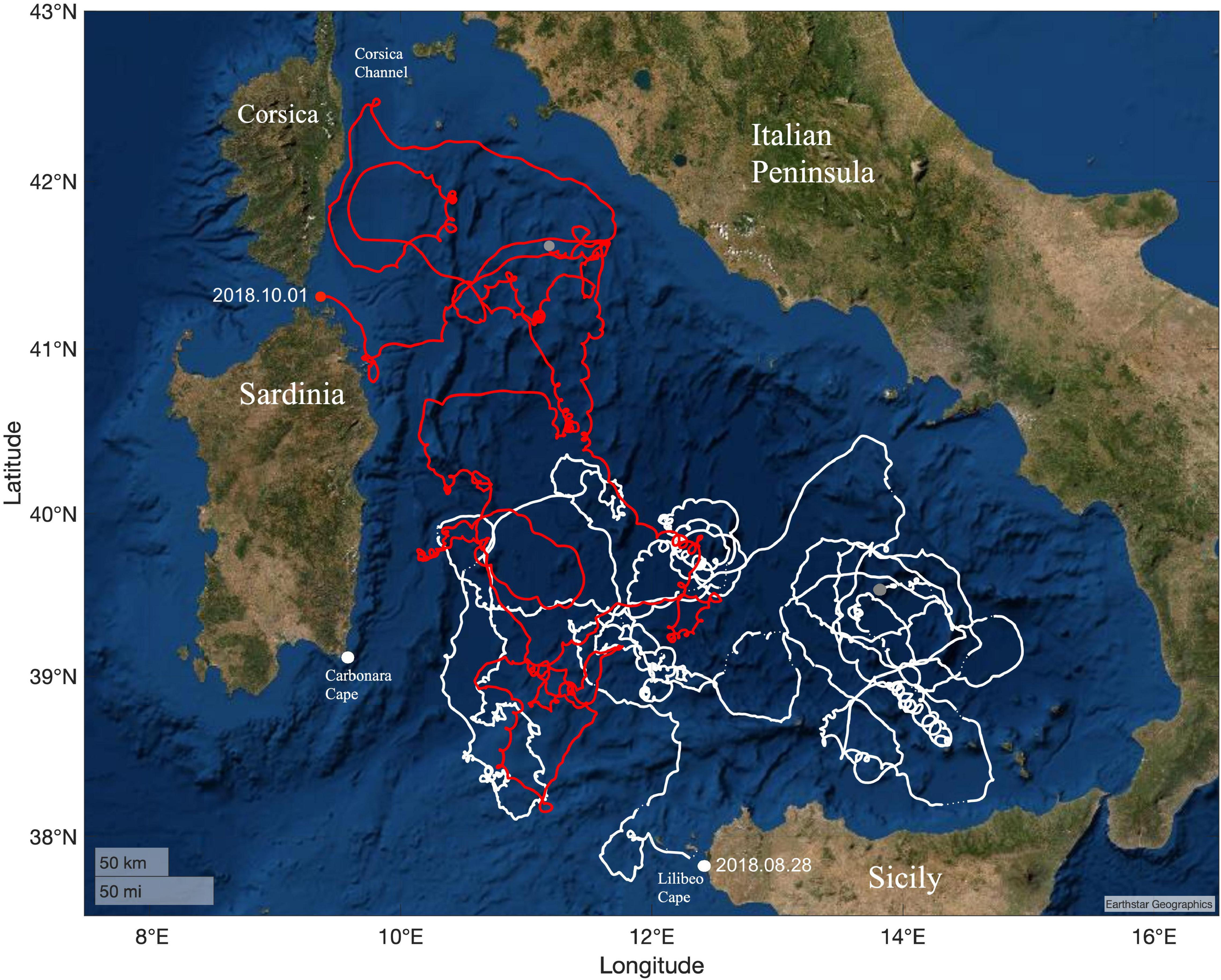
Trajectories of the loggerhead turtle (LT, white line) and of the drifter (OBS, red line). LT trajectory starts at Favignana Island (Sicily), off Lilibeo Cape, on 28 August 2018 and stops at the gray circle on 31 July 2019; the dashed white segments were excluded from the analysis (see section “Materials and Methods”). OBS trajectory starts at north Sardinia (red circle) on 1 October 2018 and stops in the northern Tyrrhenian Sea on 31 May 2019 (gray circle).
Two are the main openings toward the rest of the Mediterranean Sea: one is the south-western passage between the capes of Carbonara (Sardinia) and Lilibeo (Sicily), 290 km wide deeper at west close to Sardinia (about 2,000 m depth) than at east close to Sicily (800 m depth on average), and the other is the northern Corsica Channel, a narrow corridor between Corsica and the Tuscany Archipelago with a sill 450 m deep (Hopkins, 1988; Astraldi and Gasparini, 1994). Both contribute to regulate the general basin-scale features of the sea current circulation in the Tyrrhenian Sea (Artale et al., 1994). Two straits, the Strait of Messina and the Strait of Bonifacio also give a contribution to the Tyrrhenian Sea dynamics, locally affecting the thermohaline features of the adjacent sub-basins (Artale et al., 1994; Cucco et al., 2016).
In the Tyrrhenian Sea the amplitude of the main tidal signal, the M2 tide, is ranging between 0.1 and 0.15 m along the zonal direction (Carillo et al., 2011) with associated weak tidal currents.
A commonly adopted scheme describes the water column as characterized by a surface layer of Atlantic Water (AW), an intermediate layer of Levantine Intermediate Water and a bottom layer of resident Tyrrhenian Deep Water (Vetrano et al., 2010). The sea current general circulation can be represented by the AW entering from the southern passage and, cyclonically circulating around the basin, to partially leave the basin through the Corsica Channel and, partially, through the same southern opening along the southern Sardinian coast (e.g., Astraldi and Gasparini, 1994; Millot, 1999; Astraldi et al., 2002). During the winter season, such a flow is entering from the southern passage and intensely proceeds to the north then generating wide meanders off the northern Sicilian coasts, probably through a mechanism of baroclinic adjustment to the basin topography. By contrary, during the warmer season no intense flow of AW is found into the basin that hence shows the features of a near-isolated basin (Astraldi and Gasparini, 1994; Iacono et al., 2013).
Such a basin-scale cyclonic circulation is accompanied, in the western part of the Tyrrhenian Sea, by two quasi-permanent features, a gyre dipole off the Strait of Bonifacio (a northern cyclonic and a southern anticyclonic one) and a 200–300 km wide wind curl driven cyclonic gyre in the southeast of Sardinia, named South Eastern Sardinia Gyre (Sorgente et al., 2011). As shown by Iacono et al. (2013) and previously suggested by Pierini and Simioli (1998), this mesoscale dynamic is strongly influenced by the wind forcing and interactions with the geomorphological features of the basin. Indeed, from the edges to the interior of the basin, chlorophyll and sea surface temperature signatures reveal the existence of several gyres (Iacono et al., 2013) that are affected by seasonal inversion of the wind stress curl sign and by the winter strengthening and summer weakening of the AW stream.
This composite, multiscale ocean dynamics, including intense streams and quasi-permanent, typically cyclonic gyres (Iacono et al., 2013), is a reliable engine that is able to generate a regular nutrients transport to the euphotic zone and consequent formation of plankton aggregations areas where LT are often found, and where they can remain for long time (Luschi et al., 2018; Chimienti et al., 2020).
Materials and Methods
All methods were carried out in accordance with relevant guidelines and regulations. Manipulation and handling of the sea turtle, including transmitter attachment, were carried out under authorizations issued by the Italian Ministry of Environment (PNM. REGISTRO UFFICIALE. U. 0032115 3/10/2018 to AMP Isole Egadi; PNM. REGISTRO UFFICIALE.U. 0025257 21/11/2017 to PL).
Tracking Data Collection
The LT analysed in this study was rescued after being captured by longlines in southern Sicilian waters and remained at the sea turtle rescue center on the island of Favignana (Egadi Archipelago, western Sicily) for 3 months before being released at sea on 28 August 2018. The turtle was a large juvenile (Curved Carapace Length of 63 cm) and was equipped with a GPS unit linked to the Iridium satellite system (SeaTrkr model, Telonics, Mesa, AZ, United States) attached on the turtle’s carapace following standard procedures. SeaTrkr tags collect GPS locations using a rapid-fixing technology (Quick Fix Pseudoranging) and then transfer the acquired information through the Iridium satellite system. This technology has a comparable accuracy to the standard GPS systems (around 25 m) but the locations are determined in a shorter time than a standard GPS location (3 s vs. 30/90 s), even when a clear view of the sky is absent (Telonics Gen4 Gps User’s Manual, 2017). The accuracy of the SeaTrkr locations is strictly connected to the number and distribution of visible satellites.
To allow an accurate reconstruction of turtle’s trajectory and behavior with a high spatial and temporal resolution, the tag was set to collect one location per hour. For the following analyses, we considered the data collected in the first year of tracking, excluding data after 31 July 2019, approximately corresponding to when the turtle left the Tyrrhenian Sea.
Ocean Products
The adopted oceanographic information is derived by at-sea measurements of a floating surface drifter (OBS) and by assured quality numerical ocean modeling products (MOD) that benefit from in situ and satellite data assimilation.
Oceanographic measurements were provided by a 72 cm long drifter, by the SouthTEK Sensing Technologies company, with drogue at 1 m depth and equipped with GPS tracking and Iridium satellite coverage. As for SeaTrkr’s, SouthTEK’s accuracy is dependent on the number and distribution of visible satellites and comparable with the LT system. The drifter uses the Global Navigation Satellite System (GNSS) that refers to a constellation of satellites providing positioning and timing data to GNSS receivers with a typical accuracy of about 3 m. Along the trajectory, the GPS acquisition schedule was initially set to 0.5, then moved to 1 and finally 2 h to save battery life.
Modeling products consist of hourly fields of the modeled sea current velocity, at 1.0-m depth, which is the only available product at this temporal frequency for the time lapse of this LT trajectory. The data were released by the Copernicus Marine Environment Monitoring Service (CMEMS)1 that provides world seas oceanographic products for marine resources users. Specifically, in the Mediterranean Sea the ocean physics is modeled by the Mediterranean Forecasting System (Pinardi et al., 2003; Tonani et al., 2008), a coupled hydrodynamic-wave model providing reliable oceanographic information with horizontal resolution of about 4.5 km at 141 unevenly spaced levels. The model equations system accounts for barotropic and baroclinic pressure gradients, wave forcing, Coriolis and frictional forces and uses the atmospheric forcing produced by the European Centre for Medium-Range Weather Forecasts (ECMWF). It includes a variational data assimilation scheme that is used to make model solutions converging to observed variables of temperature, salinity and along-track satellite Sea Level Anomaly.
At present, tidal forcing is not considered in the Mediterranean Forecasting System implementation that is describing the wind-driven and thermohaline dynamics only. For this reason, we added to the analysis the hourly fields of tidal currents computed by the model TPXO7.2. Based on updated bathymetry, satellite altimetry assimilation and on a tidal data inversion package (Egbert et al., 1994; Egbert and Erofeeva, 2002), considering eight linear and non-linear harmonic tidal constituents, it provides earth-relative sea-surface elevation with about 4 km of spatial resolution at hourly frequency in the Mediterranean Sea.
Data Pre-processing and Sea Current Effect Indicators
Despite the high spatial accuracy of the LT tag, some fixes were erroneous because falling on land or defining unrealistic speed values between successive locations. Therefore, the LT locations were filtered using a predefined speed threshold of 1.2 m⋅s−1, removing 18 locations over a total of 6,172 acquired. Although the time difference between successive LT locations can reach peaks of 12 h, the median value of the sampling time is of 1.05 h. The discrete sequence of the sampling points hence defines a high-resolution trajectory whose shape may be wrongly defined if the time difference between locations is greater than median values. For this reason, sampling points with mutual temporal distance greater than 6 h (0.7% of the locations) were excluded; they were represented by dashed lines in Figures 1, 4, 7.
Finally, longitude and latitude in decimal degrees of the LT and OBS datasets were converted in meters (UTM zone 32) in order to estimate the distance between successive locations in the plane and a 1-h, piece-wise cubic interpolation procedure was carried out to get a homogeneous sequence of locations.
After this pre-processing procedure, the two components of the OBS and LT ground velocities (along the zonal and meridional axes) were inferred through the application of their cinematic formulation, hence considering the distance between two successive points and the time lag between their acquisition. Then, by separated procedures, the components of the MOD velocities, generated by tidal and composite wind-driven and thermohaline forcing, were interpolated in space and time along the discrete sequence of LT locations.
OBS, LT, and MOD velocity datasets were compared to highlight potential common features. Firstly, through basic statistical indicators and the computation of the cross-correlation, and secondly through spectral analysis to explore frequencies or periodicities of the dataset variance. Then, ad-hoc designed indicators were computed to evaluate the effects of the sea current advection along the LT trajectory, as explained in the following.
The Angle Between two Rays (ABR) is the angle between two velocity vectors at the same point and it is computed using the definition of scalar product between two vectors. ABRα was computed to assess the MOD performance in representing the observed sea current velocity (OBS), ABRβand ABRγto assess directional coherence between the MOD sea current and the LT ground velocity vectors considering the combined wind-driven and thermohaline dynamics (ABRβ) and the tidal current only (ABRγ). As an example, for the computation of the ABRβ, the scalar product read as:
from which the angle β between two vectors (ULT and UMOD) can be straightforwardly deduced. ABR can assume values between 0 and 180°, with values <90° indicating that specific components of the MOD velocities flow in the same direction of the LT ground velocity. For values around 90°, the impact of the MOD velocities can deflect the LT trajectory, while for angle >90° it can deflect the LT trajectory and reduce the module of the LT ground velocity vector.
The Sea Current Impact (SCI) indicator was used to give a quantitative information about the impact of the wind-driven and thermohaline sea current advection MOD on the LT ground velocity. At each point of the turtle route, SCI is computed as the ratio between the orthogonal projection of the MOD sea current velocity onto a tangent line passing through the considered locations and the LT ground velocity. The formulation reads as
SCI values range between 1 or −1 but can exceed this range if the MOD sea current velocity orthogonal projection has a high intensity with respect to the LT ground velocity. SCI positive values indicate that sea currents are contributing to LT ground movement while negative values show that currents are contrasting turtle movement.
The computation of the eddy kinetic energy (EKE) was also performed to identify the most energetic areas encountered by the LT along its journey in the Tyrrhenian basin. EKE is defined as the kinetic energy of the time-varying component of the velocity field that contains all processes that vary in time, including mesoscale eddies, jets, and large-scale motions (Martínez-Moreno et al., 2019). It reads as
where the varying part of the sea current velocity components are calculated as
with < > representing a time averaging along the whole length of the LT trajectory.
The MATLAB environment was used to implement all necessary data reading, analysis, and displaying tools.
Results
The new proposed aggregated methodology was tested on the study case following two successive steps: (1) the exploration of any common feature between the observed trajectory and velocities of a tracked LT and the path of a surface drifter (OBS) released in the same basin in a similar period, followed by a quantitative comparison with the sea surface currents obtained by ocean models application (MOD) along the LT and OBS trajectories; (2) the quantification of the impact of the sea current velocities, obtained from MOD, on the LT trajectory through the adoption of ad-hoc designed indicators.
Main Features of Turtle and Drifter Trajectories
The white line in Figure 1 displays, with a median sampling rate of 1.05 h, the 11-m long trajectory of the LT that was released equipped with a GPS tracking device linked to the Iridium satellite system in late August 2018 from the island of Favignana, off Cape Lilibeo (Figure 1). About 1 month later (early October 2018) one satellite drifter (OBS) was released from the northern coasts of Sardinia and, with an average sampling rate of 1.05 h, provided surface currents measurements in the Tyrrhenian Sea along an 8-months long trajectory (red line in Figure 1). Both trajectories crossed the southwest Tyrrhenian region during winter (roughly December–March).
The graphic representation of the LT and OBS trajectories highlights some common features that are evident at a wide range of temporal and spatial scales. They might be summarized in (i) wide rings, i.e., circles and arcs with dimensions comparable to the widespread, mesoscale structures of the Tyrrhenian Sea circulation (diameter 10–100 km), (ii) loops, with diameters roughly less than 10 km, (iii) vertices that might be linked to a short-period sea dynamic, (iv) long or short straight segments.
The OBS and LT trajectories were then used to infer the observed sea current velocity and the LT ground velocity. The first provided a reference for the Tyrrhenian Sea state conditions between October 2018 and May 2019 and the local reliability of the oceanographic numerical model solutions (MOD), the second described a combination of sea turtle active swimming and sea current velocities in the same basin. Oceanographic numerical models, including assimilation of in situ and remote sensing observations, were used to provide the best available representation of the sea current velocity (MOD) along the LT trajectory.
The velocities of the two observed trajectories (LT and OBS) are comparable (Table 1), then indicating that the ground velocity of this LT actually provides a reliable measure of the sea surface currents in the Tyrrhenian Sea. The MOD sea current velocities, derived at each LT location, instead seem to underestimate the observed LT ground velocity and the OBS sea current velocity (Table 1).
TABLE 1
| OBS | LT | MOD | |
| Maximum | 1.42 | 1.06 | 0.61 |
| Median | 0.20 | 0.20 | 0.13 |
| Average | 0.21 | 0.22 | 0.14 |
| Standard deviation | 0.12 | 0.12 | 0.08 |
Descriptive statistics of velocities (m⋅s−1) for OBS, LT, and MOD.
However, the cross-correlation computed as follows for LT and MOD velocities,
showed that the relation between the two datasets is not simply linear. Both signals display a phase similarity within the delay of +−2 hours but a low Pearson linear correlation coefficient (0.1952 at delay = 0).
The Power Spectrum Density Function (PSDF) was also computed for MOD and OBS sea current velocity and LT ground velocity to describe the frequency or periodicity range of the explained variance of these datasets (Figure 2). The periodogram excludes the broad energy spectrum that is derived by long periods dynamics (from days to weeks) and the noisy response below the period of 6 h. The OBS and LT datasets generally explain a high power if compared to the MOD dataset power that drastically decreases below 17 h (Figure 2). Indeed, due to the horizontal resolution of the computational grid, sub-inertial power is under-represented in the oceanographic model that fails to capture the OBS high frequency dynamics, typically influenced by the direct action of the wind drag and wave Stokes drift on the emerged part of the buoy. Nevertheless, even if underestimated, the MOD is capable to reproduce the variance of the OBS signal even at higher frequency.
FIGURE 2
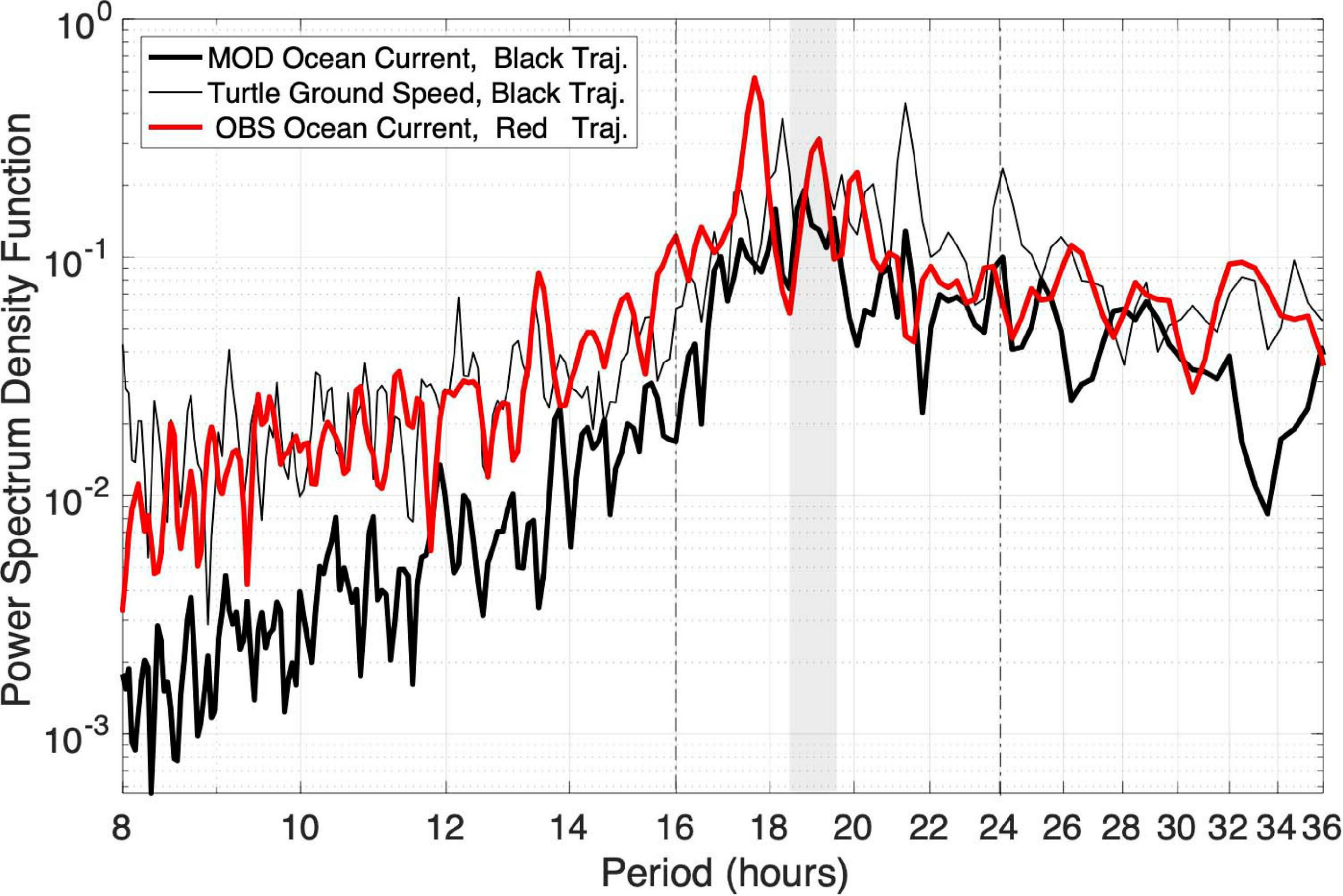
PSDF of the loggerhead turtle (LT) ground velocity (thin black line), the MOD sea current velocity (thick black line) and the OBS sea current velocity (red line). X- and y-axes are displayed in logarithmic scale. Dashed vertical lines and the gray shadow area highlight relevant periodicity ranges.
All PSDFs explain comparable power in the range between 16 and 24 h, the period of the theoretical inertial oscillations in the Mediterranean Sea. Inertial oscillations in oceanography are transitory phenomena due to the combined effect of water velocity and earth-rotation (e.g., Greenspan, 1968) and their period is given by Ti = 2π/f with f = 2Ω⋅sinϕ (i.e., two times the angular speed of earth by sin of local latitude). Considering the maximum (40.4°N) and minimum (37.7°N) latitudes of the LT trajectory ones can compute a theoretical inertial period that is hence ranging in between 18.46 and 19.56 h (Figure 2). In the PSDF the highest peaks of energy, derived from LT dataset, are found within this range of periodicity. Two more peaks are found at 21.2 and 24 h. The PSDF of MOD, derived along the LT trajectory, shows a wide peak centered at 18.5 and a tighter one centered at 21 h. The OBS trajectory reaches higher latitudes and the PSDF of this dataset shows its peak between 17 and 18 h. Two more peaks are found at 19 and 20 h.
Quantification of the Impact
A straightforward method to evaluate how sea current velocity can affect the LT ground velocity is the computation of the ABR (see “Materials and Methods”) that issued to verify the directional consistency between velocity vectors at the same application point.
ABR computation was hence carried out to assess the directional coherence between the MOD and the OBS sea surface current velocity vectors (ABRα) and between LT ground velocity and MOD sea current velocity vectors, considering the combined wind-driven and thermohaline dynamics (ABRβ) and the tidal current (ABRγ), separately.
Through this approach, if the MOD sea current velocity provides a coherent representation of the OBS velocity along the trajectory, the ABRα values would be close to zero or include small angles. Similarly, if the ABRβ or the ABRγvalues are near 90°, the current advection has a neutral impact on the module of the LT ground velocity, but it can deflect the sea turtle from any chosen route. If they are less than or greater than 90°, the sea current advection affects both the module and direction of the LT ground velocity, respectively favoring or contrasting the turtle movement.
Figure 3A displays the directional coherence between the MOD and OBS velocity vectors along the OBS trajectory: 67.9% of the ABRα values angles are below 90°, 51.5% below 60° and 28.3% below 30°. Although the directional coherence suffers from the wind drift effect, which is often hardly represented by the model’s solutions and acting on the drifter along the OBS trajectory, as also shown by Putman et al. (2020), ABRα does provide a useful assessment of the model solutions accuracy in the basin that is instrumental for the subsequent analyses.
FIGURE 3
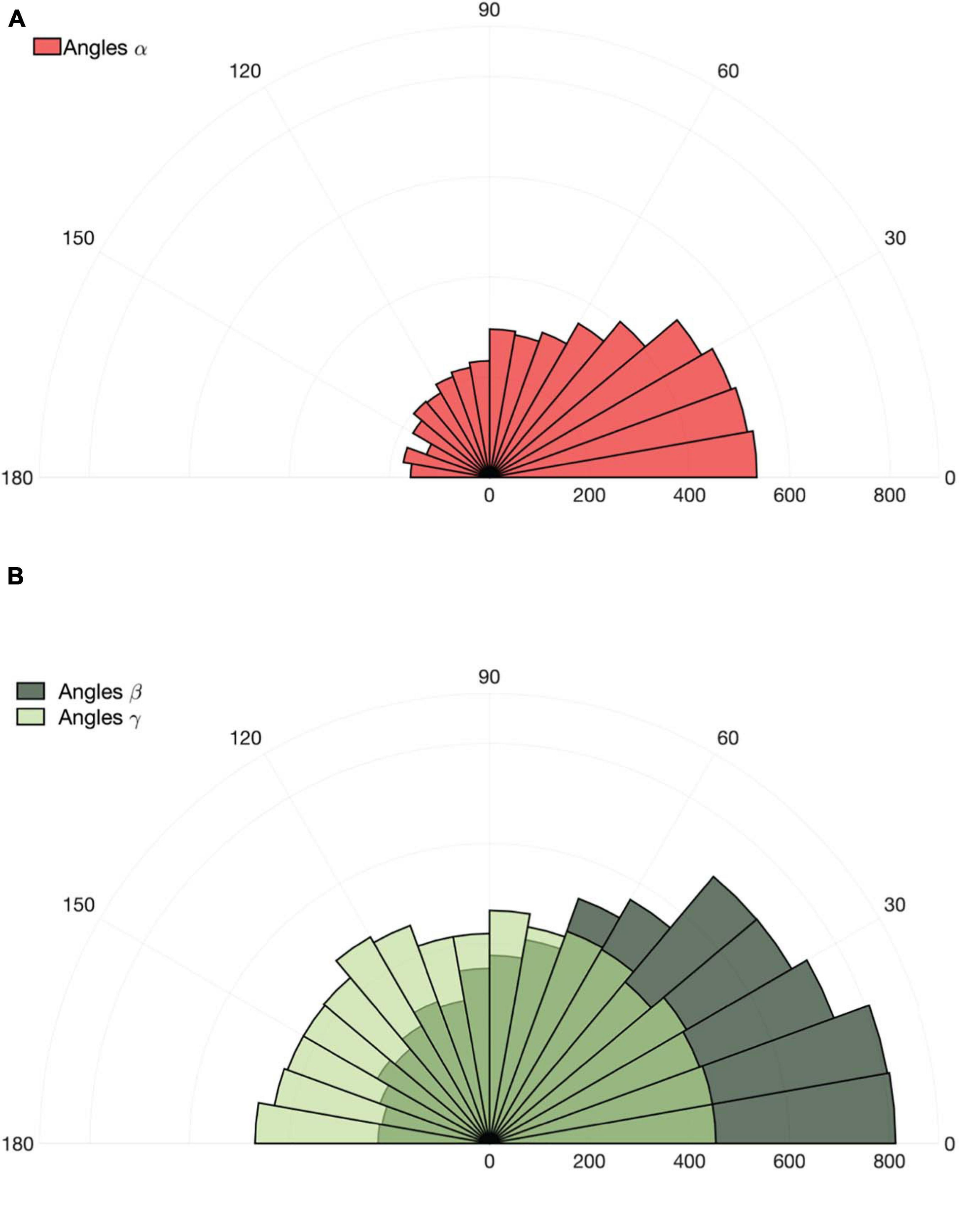
(A) Polar histograms of the angles (ABRα) between the OBS and MOD velocity vectors and (B) between the loggerhead turtle (LT) ground velocity and the MOD sea current velocity vectors (ABRβ; dark green) and between the LT ground velocity and the MOD Tidal current velocity vectors (ABRγ; light green).
Throughout the analysed LT route, 70.1% of the ABRβ values are below 90°, 53.8% are below 60° and 29.4% are below 30° (Figure 3B). Therefore, the LT ground velocity is mostly favored by the MOD sea current advection and, for about 30%, it is not favored, excluding the rare cases of feeble sea currents that oppose to the sea turtle route (i.e., ABRβ near 180°). On the other hand, the ABRγ values are uniformly distributed (Figure 3B), thus indicating a clear independency of the LT trajectory from the direction of the tidal current.
The ABRβ and ABRγvalues were also analysed with respect to LT ground velocities (Table 2). When ABRβ < 90°, the LT ground velocities were always higher than those recorded when ABRβ > 90°. This potentially highlights that the LT profits of favorable sea currents advection. The ABRγ had equivalent values across all possible angle values, demonstrating the independence of the LT ground velocity from the tidal current velocity, that is feeble in the interior of the Tyrrhenian basin.
TABLE 2
| LT ground velocity for ABRβ |
LT ground velocity for ABRγ |
|||
| 0° < ABR< 90° | 90° < ABR< 180° | 0° < ABR< 90° | 90° < ABR< 180° | |
| Maximum | 1.06 | 0.76 | 0.79 | 1.06 |
| Median | 0.21 | 0.17 | 0.20 | 0.20 |
| Average | 0.24 | 0.18 | 0.22 | 0.22 |
| Standard deviation | 0.13 | 0.10 | 0.12 | 0.12 |
Descriptive statistics of loggerhead turtle (LT) ground velocity (m⋅s−1) in relation to ABRβ and ABRγ.
A quantitative information about the impact of the MOD sea current velocity advection on the LT ground velocity was provided by the Sea Current Impact (SCI) indicator, the ratio between the orthogonal projection of the MOD sea current velocity onto a tangent line passing through the considered locations and the LT ground velocity (see Materials and Methods). When SCI is greater than zero, the MOD sea current velocity contributes to the LT ground velocity, while when SCI is less than zero, the MOD sea current velocity opposes to the LT ground velocity.
The MOD sea current advection generates different impacts on the LT route in relation to the various spatial and temporal scales of the local oceanographic features (Figure 4). Wide rings display both positive and negative SCI values (e.g., route segments 1, 2, 3, 5) and they can include short straight segments, generally displaying positive SCI values, and vertices, where large variations of the SCI values can be observed, often including a change of sign at their extreme point. Loops always display positives, and typically high, SCI values (e.g., Segment 4 in Figure 4). This kind of features are found along the whole trajectory with many different occurrences.
FIGURE 4
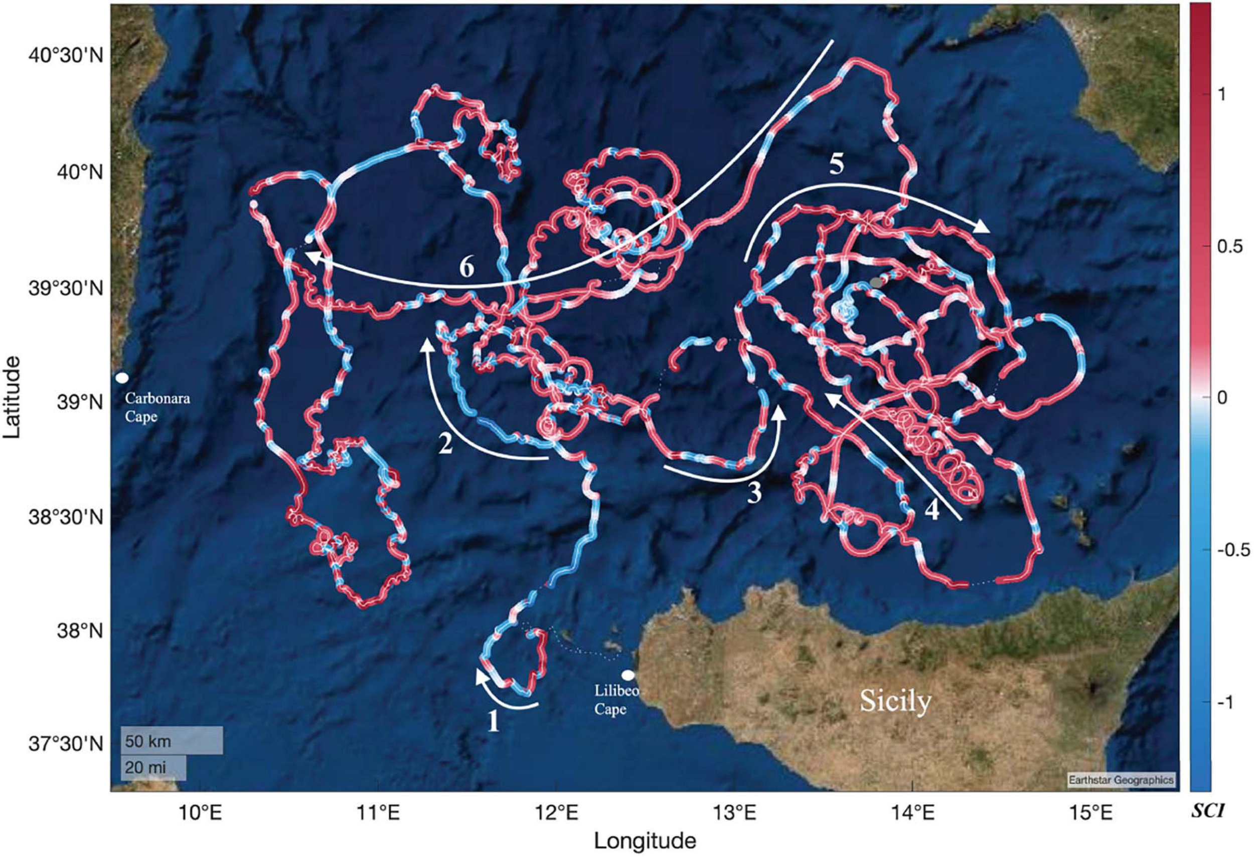
SCI values reported along the loggerhead turtle (LT) trajectory (white line). SCI is the ratio between the orthogonal projection of the MOD sea current velocity onto a tangent line passing through the considered locations and the LT ground velocity. SCI values are color-coded according to the scale on the right. Numbered arrows identify specific segments of the LT route. The white dashed line represents the portions of the LT trajectory that were excluded from the analysis. SCI values beyond the range ±1 are represented with saturated colors.
The Probability Density Function (PDF) explains the probability that SCI values fall into specific ranges. As shown in Figure 5, 54% of the locations had SCI values greater than 0 and less than 1. Thus, for the 54% of the sampling points the projected component of the MOD sea current velocity proceeds along the same direction of the LT ground velocity. The probability to find MOD sea current velocity values close to those of LT ground velocity is about 0.16. Extreme values, at both tails of the PDF are sparse along the trajectory and correspond to a combination of high MOD sea current values and low LT ground velocity values that can affect the computation of SCI values.
FIGURE 5
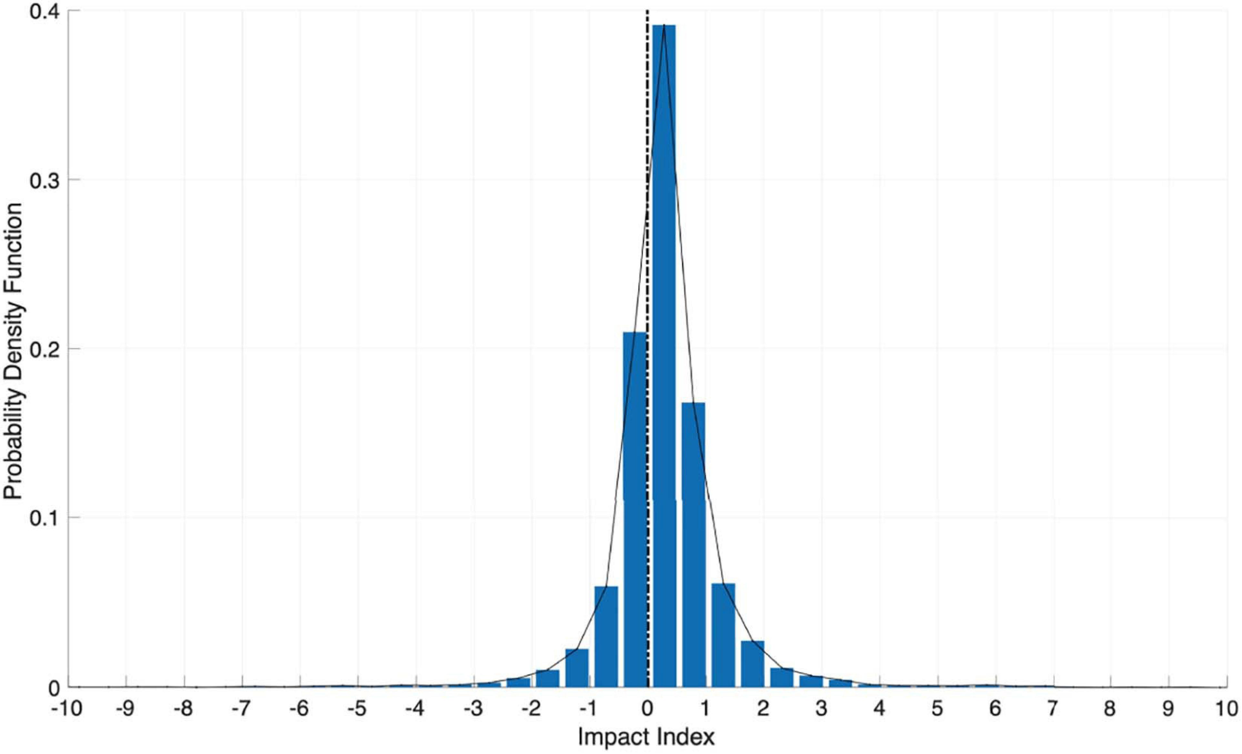
PDF of SCI values estimated along the loggerhead turtle (LT) trajectory.
Discussion
Several studies have shown that sea turtles can be affected by marine currents in their movement patterns and/or deviated from their routes in the open sea (see references in the Introduction). All these studies were carried out starting from tracks reconstructed with low-resolution tracking systems that normally have long temporal gaps and relying on low temporal and spatial resolution oceanographic information (e.g., Girard et al., 2006; Mencacci et al., 2010). In this paper, a novel aggregated methodology has been developed to investigate the influence of oceanographic features on sea turtle movements through detailed spatial and temporal representation of sea conditions. The method was successfully applied on the high-resolution trajectory of a LT, which revealed how and to which extent the tracked turtle has been affected by marine currents encountered during its oceanic movements.
Already the graphic representation of LT and OBS trajectories (Figure 1) permitted to recognize recurrent features that were strikingly similar in both cases. The courses were displaying analogous elements like wide rings, straight segments, vertices, and loops, with spatial and temporal scales that are comparable to (and likely derive from) the mesoscale and sub-mesoscale features of the Tyrrhenian Sea ocean dynamics (Iacono et al., 2013). The employment of the novel Iridium-linked GPS tracking system has been instrumental in this respect, as it has allowed to unravel detailed movements that could not be identified by previous studies using standard satellite telemetry techniques (e.g., Luschi et al., 2018) then providing the basis for the oceanographic analyses performed. The importance of relying on detailed reconstruction of turtle movements to obtain relevant information on turtle at sea behavior has indeed been underlined in recent studies employing advanced GPS tags with frequent collection of locations (Dujon et al., 2017; Chimienti et al., 2020).
The overall similarity between LT and OBS trajectories was mirrored by the common periodicities identified in the velocity datasets through the analysis of their PSDFs. Interesting similarities were found within the range of 16 and 24 h of the periodogram, the same of the inertial motions in the Mediterranean Sea (Figure 2). Velocity and shape of the analysed LT trajectory hence seems to have been linked to the short-term (days) and the inertial motions of the sea, a novel outcome that could not be highlighted without this analysis and without high frequency information about the followed path.
Along the same line, the computation of the ABRβ, computed by considering the combined wind-driven and thermohaline modeled dynamics, permitted to assess that this LT encountered favorable sea currents advection for about the 70% of the time. Conversely, ABRγ, that only takes modeled tidal forcing into account, highlighted a random impact on the LT ground velocity. This was found for the movements of this LT that took place in the interior of the Tyrrhenian Sea where tidal currents are about two orders of magnitude smaller than the LT ground velocity.
The SCI indicator was designed and adopted to quantify the impact of the MOD sea current velocity on the LT ground velocity. In most cases MOD velocities were found to concur to determine the shape of the turtle trajectory, like in correspondence of loops and vertices. It is the case of the route Segment 4 (Figure 4) where the trajectory is drawing a series of loops that reduce their diameters with time. There, positive SCI values (Figure 6A) indicate the remarkable impact of the sea current which intensity (Figure 6B) is reducing within a few days (a loop includes about 24-h samples).
FIGURE 6
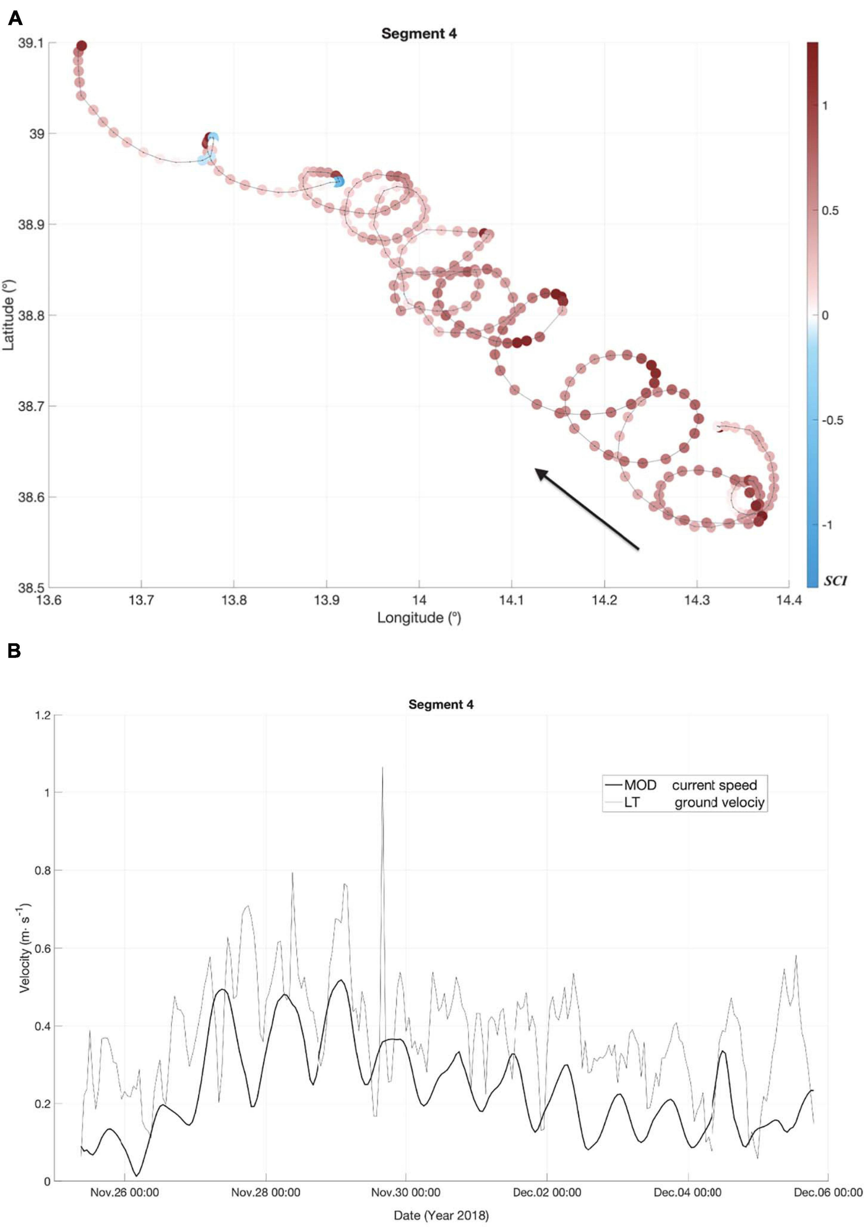
(A) Segment 4 of the loggerhead turtle (LT) trajectory (black line; see also Figure 4) with SCI values at sampling points. The black arrow indicates the general direction of the motion along this segment. (B) Intensity of LT ground velocity (thin gray line) and MOD sea current velocity (thick black line) along this segment.
The link between specific features of this LT trajectory and the energy content of the MOD sea current is exemplified by the computation of the eddy kinetic energy (EKE), the kinetic energy of the time-varying component of the sea current velocity, including mesoscale eddies, jets, and energetic large-scale motions (Shillinger et al., 2008; Martínez-Moreno et al., 2019). In Figure 7, EKEs give immediate evidence and geographical localization of the oceanic forcing that is continuously affecting, with varying strength, the LT trajectory (e.g., Segments 2 and 5). EKEs equal or greater than 10–3 are indeed extensively distributed along the trajectory.
FIGURE 7

EKE m2⋅s−2 values computed along the loggerhead turtle (LT) analysed trajectory (white line). Numbered arrows identify specific segments of the LT route. The white dashed line represents the portions of the LT trajectory that were excluded from the analysis.
For instance, EKEs equal or less than 10–2 describe the ocean energy along the east portion of the Segment 6 while the west portion displays higher EKEs that can trigger the generation of vertices and small loops. EKE values equal or greater than 10–1 are found in correspondence of the entire Segment 4, deeply affected by the occurrence of energetic marine currents advection.
On the whole, the integrated method we developed has provided detailed information on how sea currents impacted the LT movements. Given that only a single turtle was analysed as study case, it is difficult to extend such an information for all the loggerheads moving in this area. Nevertheless, it emerged that the mechanical action of current has largely contributed to shape peculiar attributes of the analysed turtle trajectory, like loops or vertices, that were remarkably similar to those found along the OBS route (Figure 1), then suggesting that current circulation patterns may play a major role for movements taking place in semi-enclosed basins like the Mediterranean Sea, in accordance with previous studies on turtles moving in the ocean (e.g., Doyle et al., 2008; Lambardi et al., 2008; Mencacci et al., 2010).
Also, the turtle did not only passively drift with the current as a drifter does, but it was able to freely swim toward a given direction. One such example is given by the Segment 6 of the LT trajectory (Figures 4, 8A), where the velocity is initially higher than MOD velocity (Figure 8B), indicating that the turtle was likely actively swimming. In the successive west portion of the segment, the turtle considerably reduces its velocity that becomes comparable to the MOD velocity values, while displaying similar short-term oscillations (Figure 8B). This reduction in turtle speed led to a radical change in the shape of the route that from linear became wavy, as a consequence of the increased weight of the current action (Figure 8A). A further example is given along the trajectory portion between Segment 1 and 2 (Figure 4), where it is reasonable to hypothesize a vigorous effort of the LT to reach the interior of the Tyrrhenian Sea. Indeed, EKE values were high in this leg and SCI showed that unfavorable sea current advection impacted the route of the LT.
FIGURE 8
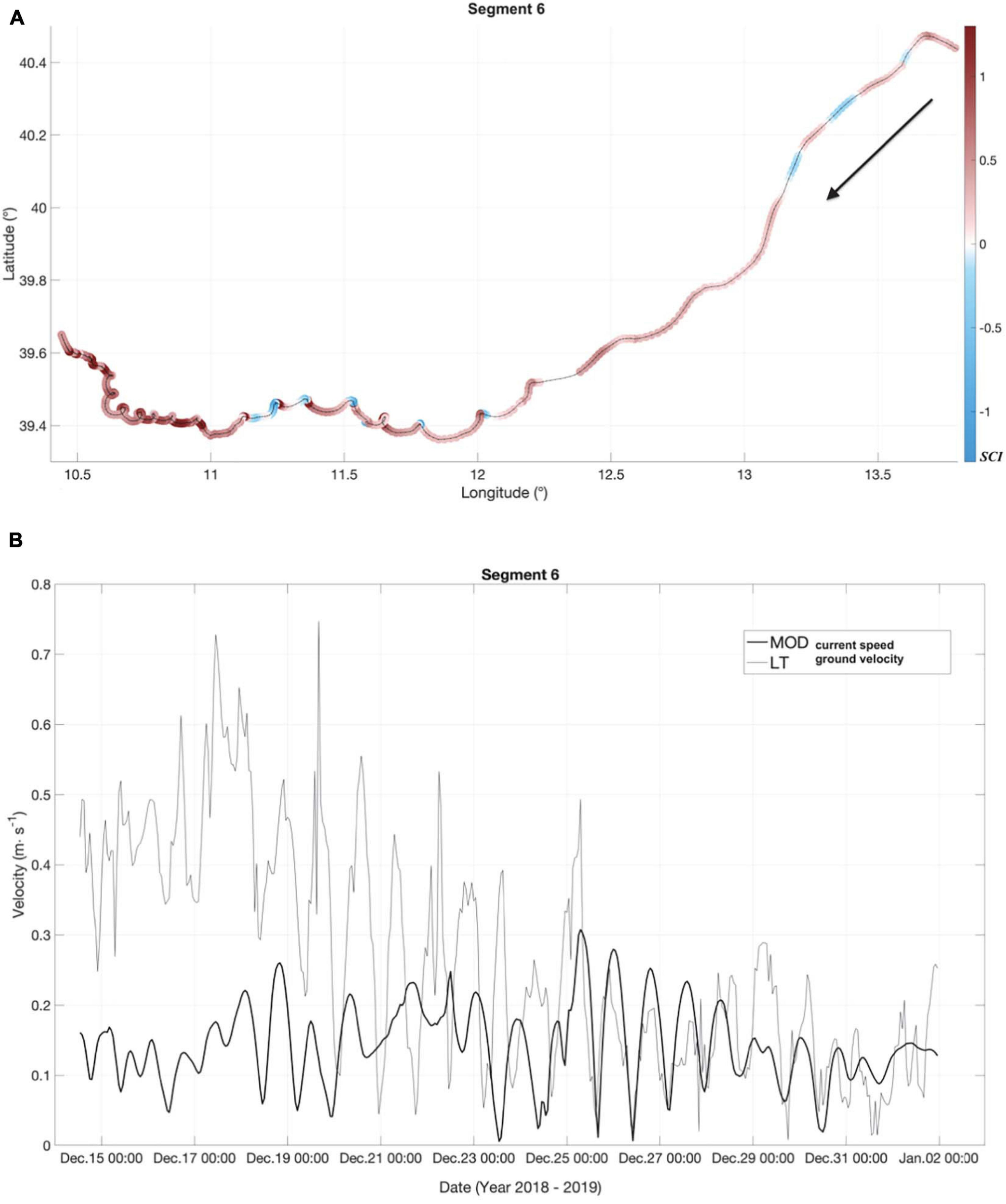
(A) Segment 6 of the loggerhead turtle (LT) trajectory (black line; Figure 4) with SCI values at sampling points. The black arrow indicates the general direction of the motion along this segment. (B) Intensity of the LT ground velocity (thin gray line) and MOD sea current velocity (thick black line) along this Segment.
However, a rigorous distinction between active swimming and sea current advection is not possible just through the presented methodology. Indeed, speed and directions of the sea current should be measured, if possible, in correspondence of the geographical location and depth at which the marine turtle is swimming. LTs are known to have a most variable diving behavior, depending on their life stage and areas frequented (Hochscheid, 2014), so that it may be not useful to attempt the determination of the loggerhead typical swimming depth that can be considered valid across different individuals.
The adoption of reliable and validated numerical oceanographic model solutions can represent a suitable alternative to at-sea measurements once its accuracy has been assessed for a specific geographical region and experimental setup.
Ideal experimental set up should involve deploying drifters with drogue at different depths and released in a temporal and spatial proximity of a tracked turtle. Drifters and LT trajectories are expected to fast diverge (Putman and Mansfield, 2015), but still permitting an evaluation of the sea current advection encountered by the turtle and of the role of wind and Stokes drift in shaping the observed trajectories. In the present case, the release at sea of the drifter was not planned in advance and, due to the specific experimental set up, it represents the motion of the first meter depth of the sea surface. Nevertheless, this comparison allowed us to highlight striking similarities in shape and ground velocities of OBS and LT trajectories. Furthermore, the analysis of OBS data also provided a general encouraging assessment of the model products, as shown by the relevant percentage of small ABRα computed angles (Figure 3A).
In this study, it is also demonstrated that the high temporal and spatial resolution of the adopted modeling system (Copernicus Marine Service, 2021a,b), that provided hourly fields of the sea surface motion, can be adopted to provide a general assessment of the sea current impact on the LT movements, also considering that the likely variable depth range, that is mostly frequented by oceanic stages of juvenile sea turtles, can be typically found in between the surface and 15 m depth (Fossette et al., 2010; Howell et al., 2010; Putman and Mansfield, 2015; Putman et al., 2016).
Conclusion
Overall, the novel analytical techniques we developed suggest a viable approach to study how oceanographic conditions can affect turtle movements, especially if used in conjunction with a high-resolution tracking system such as Iridium-GPS tags. Considering the wide spectrum of spatial and temporal oceanographic motion scales, and including inertial, seasonal and interannual periodicity that control marine life (Quattrocchi et al., 2019), the further extension of such an analysis to more turtles moving over different areas of the Mediterranean Sea is required and it would likely lead to obtain useful information on subtle behavioral strategies followed by loggerheads during their long stays in the oceanic realm.
Statements
Data availability statement
The datasets presented in this study can be found in online repositories. The names of the repository/repositories and accession number(s) can be found below: https://drive.google.com/drive/folders/1c6nuNtPCTQt04Exi2pt_IA8ibpWBLtds?usp=sharing.
Ethics statement
The animal study was reviewed and approved by Italian Ministry of Environment (PNM. REGISTRO UFFICIALE. U. 0032115 3/10/2018 to AMP Isole Egadi; PNM. REGISTRO UFFICIALE.U. 0025257 21/11/2017 to PL).
Author contributions
GQ promoted the research cooperation between all authors, conceived the research, designed, developed and applied metrics, analysis and visualizing tools before writing the entire manuscript. AC provided crucial scientific support in conceiving the research and reviewed the text of the manuscript. GCe reviewed and integrated the text of the manuscript providing constructive criticism to improve the scientific contents. RM deployed the satellite tag, processed the raw data generating the LT trajectory and reviewed the manuscript. GCo and DS provided the rescued turtle to be tracked and helped in its release at sea. AR processed the raw data generating the drifting buoy trajectory, reviewed and integrated the text of the manuscript. PL provided crucial scientific support in conceiving the research, reviewed and integrated the text of the manuscript.
Funding
The tracking project was funded by Bolton Food S.p.A.
Acknowledgments
The authors wish to thank Stefano Donati and Salvatore Livreri Console, managers of Area Marina Protetta Isole Egadi and Paolo Arena, health director of the marine turtle rescue center. The tracking project was funded by Bolton Food S.p.A. The drifter experiment was part of the activities supported by the project SOS Piattaforme e Impatti Offshore (Servizio Di Previsione Numerica Della Dispersione Di Idrocarburi Dalle Piattaforme Petrolifere Del Canale Di Sicilia E Medio Basso Adriatico), funded by the Italian Ministry of the Environment and Protection of Land and Sea with Executive Agreement PNM.REGISTRO UFFICIALE.U 000939.17-01-2017 of 17.01.2017.
Conflict of interest
The authors declare that this study received funding from Bolton Food S.p.A. The funder was not involved in the study design, collection, analysis, interpretation of data, the writing of this article or the decision to submit it for publication.
Footnotes
References
1
Artale V. Astraldi M. Buffoni G. Gasparini G. P. (1994). Seasonal variability of gyre−scale circulation in the northern Tyrrhenian Sea.J. Geophys. Res. Ocean9914127–14137. 10.1029/94jc00284
2
Astraldi M. Gasparini G. P. (1994). Circulation in the Tyrrhenian Sea.Seas. Interannu. Var. West. Mediterr. Sea46115–134. 10.1029/ce046p0115
3
Astraldi M. Gasparini G. P. Vetrano A. Vignudelli S. (2002). Hydrographic characteristics and interannual variability of water masses in the central Mediterranean: a sensitivity test for long-term changes in the Mediterranean Sea.Deep Sea Res. Part I Oceanogr. Res. Pap.49661–680. 10.1016/s0967-0637(01)00059-0
4
Benson S. R. Eguchi T. Foley D. G. Forney K. A. Bailey H. Hitipeuw C. et al (2011). Large−scale movements and high−use areas of western Pacific leatherback turtles, Dermochelys coriacea.Ecosphere21–27.
5
Briscoe D. K. Parker D. M. Bograd S. Hazen E. Scales K. Balazs G. H. et al (2016). Multi-year tracking reveals extensive pelagic phase of juvenile loggerhead sea turtles in the North Pacific.Mov. Ecol.41–12.
6
Carillo A. Napolitano E. Leuzzi G. Monti P. Lanucara P. Ruggiero V. et al (2011). Valutazione del Potenziale Energetico delle Correnti Marine del Mar mediterraneo.Rep. RdS/2011/65.Kista: ENEA Technical Report.
7
Casale P. Broderick A. C. Freggi D. Mencacci R. Fuller W. J. Godley B. J. et al (2012). Long-term residence of juvenile loggerhead turtles to foraging grounds: a potential conservation hotspot in the Mediterranean.Aquat. Conserv. Mar. Freshw. Ecosyst.22144–154. 10.1002/aqc.2222
8
Chimienti M. Blasi M. F. Hochscheid S. (2020). Movement patterns of large juvenile loggerhead turtles in the Mediterranean Sea: ontogenetic space use in a small ocean basin.Ecol. Evol.106978–6992. 10.1002/ece3.6370
9
Copernicus Marine Service (2021a). Available online at: https://catalogue.marine.copernicus.eu/documents/PUM/CMEMS-MED-PUM-006-004.pdf(accessed Jun11, 2021).
10
Copernicus Marine Service (2021b). Available online at: https://catalogue.marine.copernicus.eu/documents/QUID/CMEMS-MED-QUID-006-004.pdf(accessed Jun 11, 2021).
11
Cucco A. Quattrocchi G. Olita A. Fazioli L. Ribotti A. Sinerchia M. et al (2016). Hydrodynamic modelling of coastal seas: the role of tidal dynamics in the Messina Strait, Western Mediterranean Sea.Nat. Hazards Earth Syst. Sci161553–1569. 10.5194/nhess-16-1553-2016
12
Doyle T. K. Houghton J. D. R. O’Súilleabháin P. F. Hobson V. J. Marnell F. Davenport J. et al (2008). Leatherback turtles satellite-tagged in European waters.Endanger. Species Res.423–31. 10.3354/esr00076
13
Dujon A. M. Schofield G. Lester R. E. Esteban N. Hays G. C. (2017). Fastloc-GPS reveals daytime departure and arrival during long-distance migration and the use of different resting strategies in sea turtles.Mar. Biol.1641–14. 10.1080/08927014.1999.9522838
14
Egbert G. D. Bennett A. F. Foreman M. G. G. (1994). TOPEX/POSEIDON tides estimated using a global inverse model.J. Geophys. Res. Ocean9924821–24852. 10.1029/94JC01894
15
Egbert G. D. Erofeeva S. Y. (2002). Efficient inverse modeling of barotropic ocean tides.J. Atmos. Ocean. Technol.19183–204. 10.1175/1520-04262002019<0183:EIMOBO<2.0.CO;2
16
Fossette S. Girard C. López-Mendilaharsu M. Miller P. Domingo A. Evans D. et al (2010). Atlantic leatherback migratory paths and temporary residence areas.PLoS One5:e13908. 10.1371/journal.pone.0013908
17
Gaspar P. Georges J.-Y. Fossette S. Lenoble A. Ferraroli S. Le Maho Y. (2006). Marine animal behaviour: neglecting ocean currents can lead us up the wrong track.Proc. R. Soc. B Biol. Sci.2732697–2702. 10.1098/rspb.2006.3623
18
Girard C. Sudre J. Benhamou S. Roos D. Luschi P. (2006). Homing in green turtles Chelonia mydas: oceanic currents act as a constraint rather than as an information source.Mar. Ecol. Prog. Ser.322281–289. 10.3354/meps322281
19
Godley B. J. Blumenthal J. M. Broderick A. C. Coyne M. S. Godfrey M. H. Hawkes L. A. et al (2008). Satellite tracking of sea turtles: where have we been and where do we go next?Endanger. Species Res.43–22. 10.3354/esr00060
20
Greenspan H. P. (1968). The Theory of Rotating Fluids.London: CUP Archive.
21
Hochscheid S. (2014). Why we mind sea turtles’ underwater business: a review on the study of diving behavior.J. Exp. Mar. Bio. Ecol.450118–136. 10.1016/j.jembe.2013.10.016
22
Hopkins T. S. (1988). Recent observations on the intermediate and deep-water circulation in the Southern Tyrrhenian Sea.Oceanol. Acta941–50.
23
Howell E. A. Dutton P. H. Polovina J. J. Bailey H. Parker D. M. Balazs G. H. (2010). Oceanographic influences on the dive behavior of juvenile loggerhead turtles (Caretta caretta) in the North Pacific Ocean.Mar. Biol.1571011–1026. 10.1007/s00227-009-1381-0
24
Iacono R. Napolitano E. Marullo S. Artale V. Vetrano A. (2013). Seasonal variability of the tyrrhenian sea surface geostrophic circulation as assessed by altimeter data.J. Phys. Oceanogr.431710–1732. 10.1175/JPO-D-12-0112.1
25
IOC, IHO, and BODC (2003). Centenary Edition of the GEBCO Digital Atlas”, published on CD-ROM on behalf of the Intergovernmental Oceanographic Commission and the International Hydrographic Organization as part of the General Bathymetric Chart of the Oceans.Liverpool: British Oceanographic Data Centre.
26
Lambardi P. Lutjeharms J. Mencacci R. Hays G. Luschi P. (2008). Influence of ocean currents on long-distance movement of leatherback sea turtles in the Southwest Indian Ocean.Mar. Ecol. Prog. Ser.353289–301. 10.3354/meps07118
27
Luschi P. Benhamou S. Girard C. Ciccione S. Roos D. Sudre J. et al (2007). Marine turtles use geomagnetic cues during open-sea homing.Curr. Biol.17126–133. 10.1016/j.cub.2006.11.062
28
Luschi P. Casale P. (2014). Movement patterns of marine turtles in the Mediterranean Sea: a review.Ital. J. Zool.81478–495. 10.1080/11250003.2014.963714
29
Luschi P. Hays G. C. Papi F. (2003). A review of long−distance movements by marine turtles, and the possible role of ocean currents.Oikos103293–302. 10.1034/j.1600-0706.2003.12123.x
30
Luschi P. Mencacci R. Cerritelli G. Papetti L. Hochscheid S. (2018). Large-scale movements in the oceanic environment identify important foraging areas for loggerheads in central Mediterranean Sea.Mar. Biol.1651–8. 10.1109/joe.2020.3045645
31
Mansfield K. L. Wyneken J. Porter W. P. Luo J. (2014). First satellite tracks of neonate sea turtles redefine the ‘lost years’ oceanic niche.Proc. R. Soc. B Biol. Sci.281:20133039. 10.1098/rspb.2013.3039
32
Martínez-Moreno J. Hogg A. M. Kiss A. E. Constantinou N. C. Morrison A. K. (2019). Kinetic energy of eddy-like features from sea surface altimetry.J. Adv. Model. Earth Syst.113090–3105. 10.1029/2019MS001769
33
Mencacci R. De Bernardi E. Sale A. Lutjeharms J. R. E. Luschi P. (2010). Influence of oceanic factors on long-distance movements of loggerhead sea turtles displaced in the southwest Indian Ocean.Mar. Biol.157339–349. 10.1007/s00227-009-1321-z
34
Millot C. (1999). Circulation in the Western Mediterranean Sea.J. Mar. Syst.20423–442. 10.1016/S0924-7963(98)00078-5
35
Pierini S. Simioli A. (1998). A wind-driven circulation model of the Tyrrhenian Sea area.J. Mar. Syst.18161–178. 10.1016/s0924-7963(98)00010-4
36
Pinardi N. Allen I. Demirov E. De Mey P. Korres G. Lascaratos A. et al (2003). The Mediterranean ocean forecasting system: first phase of implementation (1998-2001).Ann. Geophys.213–20. 10.5194/angeo-21-3-2003
37
Putman N. F. Lumpkin R. Olascoaga M. J. Trinanes J. Goni G. J. (2020). Improving transport predictions of pelagic Sargassum.J. Exp. Mar. Bio. Ecol.529:151398. 10.1016/j.jembe.2020.151398
38
Putman N. F. Lumpkin R. Sacco A. E. Mansfield K. L. (2016). Passive drift or active swimming in marine organisms?Proc. R. Soc. B Biol. Sci.283:20161689. 10.1098/rspb.2016.1689
39
Putman N. F. Mansfield K. L. (2015). Direct evidence of swimming demonstrates active dispersal in the sea turtle “Lost Years.”.Curr. Biol.251221–1227. 10.1016/j.cub.2015.03.014
40
Quattrocchi G. Sinerchia M. Colloca F. Fiorentino F. Garofalo G. Cucco A. (2019). Hydrodynamic controls on connectivity of the high commercial value shrimp Parapenaeus longirostris (Lucas, 1846) in the Mediterranean Sea.Sci. Rep.9:16935. 10.1038/s41598-019-53245-8
41
Robinson N. J. Morreale S. J. Nel R. Paladino F. V. (2016). Coastal leatherback turtles reveal conservation hotspot.Sci. Rep.6:37851. 10.1038/srep37851
42
Shillinger G. L. Palacios D. M. Bailey H. Bograd S. J. Swithenbank A. M. Gaspar P. et al (2008). Persistent leatherback turtle migrations present opportunities for conservation.PLoS Biol.6:e171. 10.1371/journal.pbio.0060171
43
Sorgente R. Olita A. Oddo P. Fazioli L. Ribotti A. (2011). Numerical simulation and decomposition of kinetic energy in the Central Mediterranean: insight on mesoscale circulation and energy conversion.Ocean Sci.7503–519. 10.5194/os-7-503-2011
44
Telonics Gen4 Gps User’s Manual (2017). Available online at: https://www.telonics.com/manuals.php(accessed July 8, 2021).
45
Tonani M. Pinardi N. Dobricic S. Pujol I. Fratianni C. (2008). A high-resolution free surface model on the Mediterranean Sea.Ocean Sci.41–14. 10.5194/os-4-1-2008
46
Vetrano A. Napolitano E. Iacono R. Schroeder K. Gasparini G. P. (2010). Tyrrhenian Sea circulation and water mass fluxes in spring 2004: observations and model results.J. Geophys. Res.115:C06023. 10.1029/2009JC005680
Summary
Keywords
loggerhead turtle, marine turtle trajectories, ocean motions, sea current impacts, hydrodynamic controls, Mediterranean Sea
Citation
Quattrocchi G, Cucco A, Cerritelli G, Mencacci R, Comparetto G, Sammartano D, Ribotti A and Luschi P (2021) Testing a Novel Aggregated Methodology to Assess Hydrodynamic Impacts on a High-Resolution Marine Turtle Trajectory. Front. Mar. Sci. 8:699580. doi: 10.3389/fmars.2021.699580
Received
23 April 2021
Accepted
29 June 2021
Published
22 July 2021
Volume
8 - 2021
Edited by
Stefano Aliani, Consiglio Nazionale delle Ricerche, Institute of Marine Science U.O.S. of Pozzuolo di Lerici, Italy
Reviewed by
Robert Marsh, University of Southampton, United Kingdom; Nathan Freeman Putman, LGL, United States; Robert Hardy, National Marine Fisheries Service (NOAA), United States
Updates
Copyright
© 2021 Quattrocchi, Cucco, Cerritelli, Mencacci, Comparetto, Sammartano, Ribotti and Luschi.
This is an open-access article distributed under the terms of the Creative Commons Attribution License (CC BY). The use, distribution or reproduction in other forums is permitted, provided the original author(s) and the copyright owner(s) are credited and that the original publication in this journal is cited, in accordance with accepted academic practice. No use, distribution or reproduction is permitted which does not comply with these terms.
*Correspondence: Andrea Cucco, andrea.cucco@cnr.it
This article was submitted to Marine Ecosystem Ecology, a section of the journal Frontiers in Marine Science
Disclaimer
All claims expressed in this article are solely those of the authors and do not necessarily represent those of their affiliated organizations, or those of the publisher, the editors and the reviewers. Any product that may be evaluated in this article or claim that may be made by its manufacturer is not guaranteed or endorsed by the publisher.