Best Practice Data Standards for Discrete Chemical Oceanographic Observations

Introduction

Standards for reporting both data and metadata are important for data sharing, quality control (QC), and synthesis efforts (Tanhua et al., 2019; Brett et al., 2020). Metadata are structured information that describes an information resource such as an oceanographic data set, providing context for it, and enabling its discovery and access (Guenther and Radebaugh, 2004; Riley, 2017). Metadata conforming to community-driven standards, such as those described by Jiang et al. (2015a) for ocean acidification data, should accompany any oceanographic data to allow them to be documented in a manner that best serves the scientific needs of users. The present paper introduces data standards for chemical oceanographic observations from discrete water samples. Specifically, standards are presented for (a) column header abbreviations, (b) quality control flags, (c) missing value indicators, and (d) calculations for certain properties and parameters.

Tabular data formats have been widely used for data preparation and submission. The column header abbreviation standards presented here are based on the 30-year-old Exchange format of the World Ocean Circulation Experiment (WOCE) Hydrographic Program (Joyce and Corry, 1994; Swift and Diggs, 2008) with updates and refinements by the Climate and Ocean-Variability, Predictability, and Change (CLIVAR) and the Carbon Hydrographic Data Office (CCHDO) of the Scripps Institution of Oceanography. This format has been used as a data file standard for discrete chemical oceanographic observations over the past several decades.

The principal motivations for this column header standard update are:

(1) The need to remove ambiguity from column headers. Three decades ago, the need for abbreviations that were machine-readable by software and tools at that time (e.g., length restrictions of six characters) led to suboptimal, and occasionally, enigmatic column headers. Examples are the use of SALNTY for Salinity and TRITER for Tritium error. Such oddly abbreviated terms may cause confusion among data users, especially those who are new to the subject area.

(2) The need for abbreviations that are consistent from quantity to quantity. For example: (a) the abbreviation for Dissolved Organic Carbon is DOC, but that for Dissolved Inorganic Carbon is TCARBN instead of DIC; (b) the abbreviation for Nitrate is NITRAT, but for Ammonium, it is NH4 instead of AMMONI; (c) the abbreviation for Δ¹⁴C of DOC is 14C-DOC, but for the Δ¹⁴C of DIC it is DELC14 instead of 14C-DIC; (d) the word “number” is abbreviated as NO in CASTNO (cast number) but as NBR in BTLNBR (Niskin bottle number).

(3) The need to improve documentation that could eliminate the potential misuse of some labels. For example, there is scant information for abbreviations such as BIONBR, PPHYTN, REFTMP, REVPRS, and NEONER, to name but a few. Also, the unit for isotope radioactivity, DM/0.1MG, is ambiguous, as it could be interpreted as decimeter/(0.1 mg), instead of its appropriate designation as disintegrations per minute (dpm)/[0.1 megagram (10⁵ g)], or dpm/(100 kg).

(4) The need to have appropriate headers accepted by the international chemical oceanographic community and published in peer-reviewed papers to promote their broader usage.

In this collaborative effort, updated standards are developed with goals of creating clear and consistent column headers, providing documentation for the community, and promoting their international usage. The Exchange format is retained wherever it is appropriate, but improved nomenclature for properties and parameters are created when they are more descriptive and/or can improve abbreviation clarity. Note that the recommended abbreviations in this paper are narrowly designed for column headers. We recognize that the community has been using many conventions for some of these parameters in other situations, such as mathematical equations. We view this as a separate topic and do not discuss it.

The use of “content” to imply per unit mass of seawater is recommended over “concentration” that refers to the amount of solute present per unit volume of solution (Macintyre, 1976; Cvitas, 1996; IUPAC, 2014). For example, either “nitrate content” or “substance content of nitrate” is recommended instead of “nitrate concentration.” Finally, the use of quality control (QC) flags is simplified by consolidating the three WOCE QC flag tables into a single flagging scheme, omitting flags that are either obsolete or rarely used. Standardized missing value indicators are also recommended.

In addition, tools are presented to standardize calculations of derived oceanographic properties and parameters. Oceanographers often use two of the traditionally measured seawater carbon dioxide (CO₂) system parameters [namely, total dissolved inorganic carbon content (DIC), total alkalinity content (TA), pH, and carbon dioxide partial pressure (pCO₂) or fugacity (fCO₂)] to compute the complete carbonate system using a program such as CO2SYS. CO2SYS was initially developed by Lewis and Wallace (1998) and it was later adapted for Microsoft Excel and MATLAB by Pierrot et al. (2006). The code was vectorized, refined, and optimized for computational speed by van Heuven et al. (2011) as a MATLAB program. These carbonate chemistry calculations, based on thermodynamic equilibria, are now available in a dozen public computer packages. Orr et al. (2015) compared ten of them using common input data and the set of equilibrium constants then recommended for best practices. All packages calculate values that agreed within 0.2 μatm for fCO₂, 0.0002 units for pH, and 0.1 μmol kg^–1 for carbonate ion content ([CO₃^2–]), in terms of surface zonal-mean values, although the overall uncertainties of such calculated quantities were much larger. Options for error propagation (included in the original CO2SYS) were added recently by Orr et al. (2018) to CO2SYS-Excel (Visual Basic), CO2SYS-MATLAB (MATLAB), seacarb (R), and mocsy (Fortran).

Some laboratories have begun to include carbonate ion content ([CO₃^2–]) as an additional measurable parameter of the seawater CO₂ system (Byrne and Yao, 2008; Sharp and Byrne, 2019). In this study, we report upgraded CO2SYS programs (available in Excel, MATLAB/GNU Octave, and Python) and the R package seacarb that accept [CO₃^2–], as well as [HCO₃^–] (bicarbonate ion content), and [CO₂*] (the sum of dissolved carbon dioxide [CO_2(aq)] and carbonic acid content [H₂CO₃]) as input variables. These additions to the CO₂ system calculation programs now allow adjustment of measured [CO₃^2–] to in situ conditions, and calculation of other seawater CO₂ system parameters.

By standardizing column headers, quality control flags, missing value indicators, and offering tools to standardize calculations of certain derived properties for the international chemical oceanographic community, this work will promote the use of chemical oceanographic data files in a uniform and consistent format. This will aid in the subsequent sharing of chemical oceanographic data, facilitate submission of data into permanent archives, promote future quality control and synthesis efforts, and help advance science in the field of chemical oceanography.

Column Header Abbreviation Standards

The updated column header abbreviations for discrete chemical oceanographic data (Table 1) are created in accordance with the following considerations:

TABLE 1

Table 1. Recommended column header abbreviations, their corresponding WOCE Exchange format terms (in italic), recommended units, and brief descriptions, for discrete chemical oceanographic observations.

(a) Prior usage by the international chemical oceanographic research community.

(b) Use of abbreviations that provide more information or greater clarity, for example, Silicate instead of SILCAT, Salinity instead of SALNTY.

(c) Use of both upper and lower cases in the abbreviations.

(d) Documentation for every abbreviation.

These abbreviations are discussed below in the order in which they appear Table 1. Their corresponding CCHDO Exchange format terms are listed in the second column of Table 1. The Global Ocean Data Analysis Product (GLODAP) (Olsen et al., 2020) and Climate and Forecast (CF) (Hassell et al., 2017) terms are listed in Supplementary Table 2.

Expedition codes (EXPOCODE) uniquely identify specific voyages. These codes are composed of the four-character ship code of the International Council for the Exploration of the Sea (ICES) and the date of departure from port (Coordinated Universal Time, or UTC) using ISO-8601 format (YYYYMMDD) (Table 1). For example, a research expedition onboard National Oceanic and Atmospheric Administration (NOAA) Ship Ronald H. Brown (ICES code: 33RO) leaving the port on August 27, 2015 (Coordinated Universal Time, or UTC) would have an EXPOCODE of 33RO20150827. In rare cases, if a ship leaves on a single day for multiple expeditions, the two-digit hour of departure from port (24-h format) can also be appended to the EXPOCODE with an extra “H” (hour) before the two-digit hour (e.g., 33RO20150827H15). The ICES ship code can be accessed through https://vocab.ices.dk. If the utilized vessel does not have an ICES ship code, one can be obtained from either ICES or NOAA’s National Centers for Environmental Information (NCEI).

Cruise identification (Cruise_ID) is the particular ship cruise identifier or other alias for a cruise (Table 1). It is recommended that Cruise_IDs be based on the abbreviation of the cruise section/leg and the year when the leg is visited (YYYY). For example, WCOA2007 would be the Cruise_ID of a West Coast Ocean Acidification (WCOA) cruise leg in 2007. It is recommended that all capitals be used and that hyphens, underscores, and spaces be avoided, so as to avoid multiple variations of the same cruise identifier. Exceptions can be made if an agency, institute, or research vessel has adopted a system of cruise IDs in the past and it is important to maintain historical consistency, as long as the identifiers are unique.

A sampling station is defined as a geographical location where researchers either measure properties at the site or collect samples, frequently using a conductivity, temperature, depth (CTD) rosette system (Figure 1), for later analysis in a laboratory. Station identifiers (Station_ID) can be assigned in several ways. For instance, they can be pre-assigned for a certain location and repeatedly used for cruises along the same transect, or they can be assigned sequentially. The use of all-numerical Station_IDs (Table 1) is recommended, because they are often used to split the data package into individual station units during the subsequent QC procedures and this is more easily done when Station_IDs are numbers. However, Station_IDs composed of text strings are also acceptable.

FIGURE 1

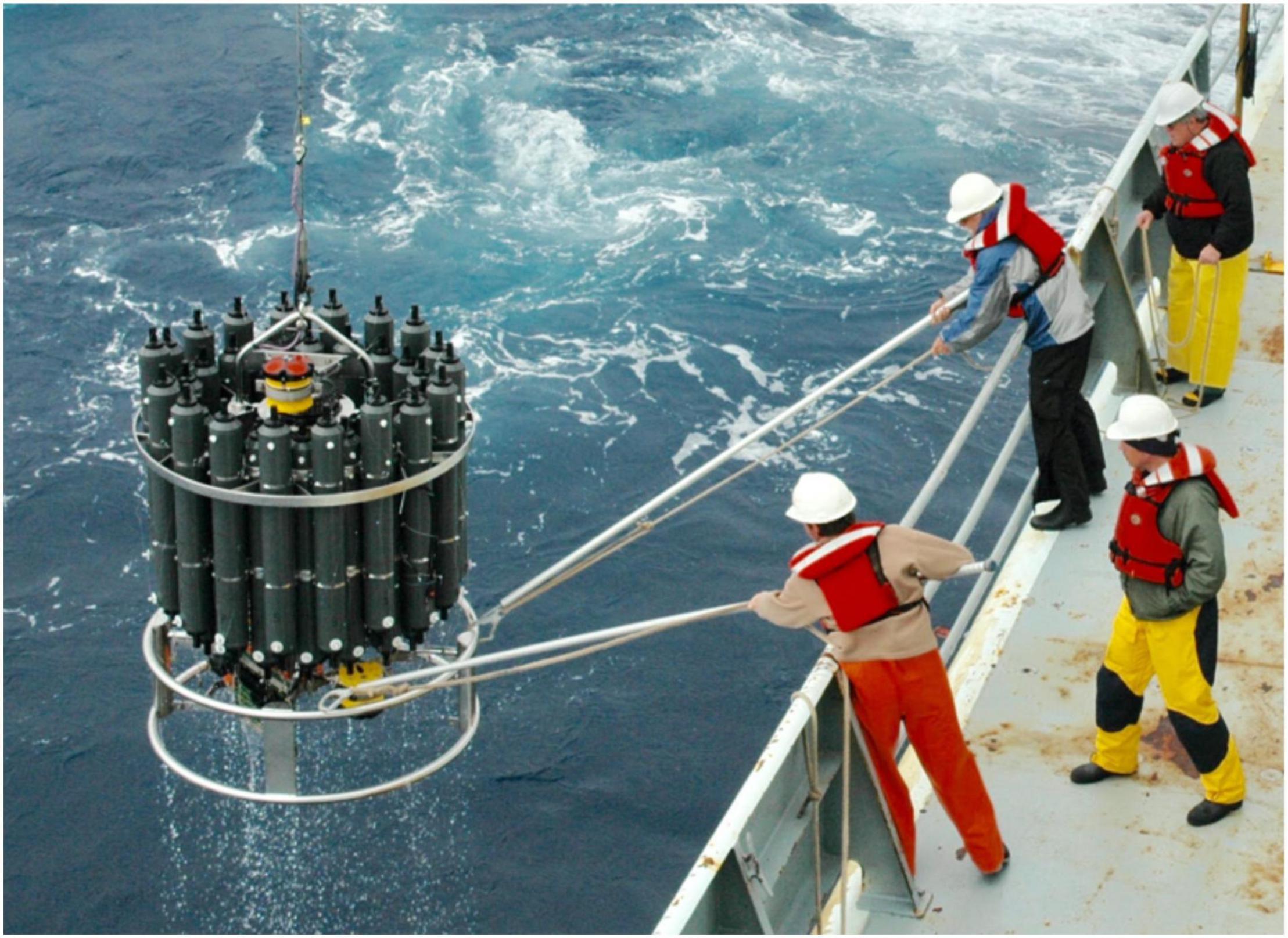
Figure 1. A rosette sampler with Niskin bottles. The conductivity, temperature, depth (CTD) sonde is inside of the ring near the bottom (not visible) (Photo credit: Sabine Mecking, University of Washington).

A new Cast_number should be used each time an over-the-side operation occurs (Table 1). Such an operation may involve deployment of a CTD rosette (Figure 1) to profile the water column, but a cast may also involve any other operation such as use of Bongo nets, standalone optical instruments, a towed array, or a pump for trace-metal sampling. Cast_number should be sequential and restart with 1 for each station when they are generated (e.g., station 1, cast 1; station 1, cast 2; station 2, cast 1; and station 3, cast 1). The use of sequential cast numbers across all stations for the entire cruise is discouraged. Another acceptable way of dealing with the Station_ID and Cast_number scheme is to avoid the use of Cast_number entirely and treat all casts as new stations.

A sample identifier (Sample_ID), which uniquely identifies a row of data during the subsequent QC and interpretation process (Table 1), is often generated by concatenating the Station_ID, Cast_number, and Rosette_position using Eq. 1:

$\mathrm{Sample}\mathrm{\_}\mathrm{ID}=\mathrm{Station}\mathrm{\_}\mathrm{ID}\times 10000+\mathrm{Cast}\mathrm{\_}\mathrm{number}\times 100+\mathrm{Rosette}\mathrm{\_}\mathrm{position}(1)$

For example, at station 15, the 2nd cast, a Rosette_position of 3 will have a Sample_ID of 150203. For samples that are not collected with Niskin bottles, such as surface samples collected via pumping or flow-through systems, or samples with non-numerical Station_IDs, Sample_ID can be filled up with unique numerical numbers as long as they do not overlap with existing Sample_IDs from the same cruise. It is recommended that each data row have a unique Sample_ID. This makes it easier to pinpoint a row when communicating with data providers and allows QC tools to generate statistics about what has been changed during the QC process. Sample_IDs can potentially be linked to persistent identifiers, e.g., International Geo Sample Numbers (IGSNs) (Plomp, 2020).

All date and time information should be in UTC. Cruise reports should record all time information in UTC; this will avoid propagation of complex shifts in the ship’s local time zone(s) into the databases. It is not necessary to report the local time (LT) as an additional column in a data file. However, it is a good practice to record the time zone(s) that the ship was in, and the time difference in hours between local time and UTC (e.g., local time from stations 1–40 was UTC – 4, and for stations 41–95, UTC – 3, etc.) in cruise reports. This is particularly necessary for biological, physical, and biogeochemical parameters that are influenced by the diurnal cycle.

Date in UTC should be reported as separate year, month, and day values (each in its own column, a total of three columns), instead of a combined date column, so as to reduce confusion caused by different date formats (e.g., international vs. United States format). Yearday_UTC refers to the day number, including a fractional component, in an annual cycle, calculated using Eq. (2):

$\mathrm{Yearday}\mathrm{\_}\mathrm{UTC}=\mathrm{datefun}(\mathrm{Year}\mathrm{\_}\mathrm{UTC},\mathrm{Month}\mathrm{\_}\mathrm{UTC},\mathrm{Day}\mathrm{\_}\mathrm{UTC})-\mathrm{datefun}(\mathrm{Year}\mathrm{\_}\mathrm{UTC},1,1)+\mathrm{Time}\mathrm{\_}\mathrm{UTC}+1(2)$

Where, “datefun” is the date function of a program (e.g., in Excel, datefun would be “DATE”). These functions convert year, month, and day into an integer where 1 day is equal to 1. Two digits after the decimal point are recommended, providing a resolution in time of 14 min. For example, 18:00 on January 1 means a Yearday_UTC of 1.75, and 06:00 on December 31 of a leap year means a Yearday_UTC of 366.25. Note that Yearday_UTC starts with 1, instead of 0. Yearday_UTC is often incorrectly called Julian Day by oceanographers and meteorologists. Julian Day is the count starting from noon on January 1, 4713 BC (UTC), and starts with 0, instead of 1. For example, January 5, 2021 has a Yearday_UTC of 5, but a Julian Day of 2,459,220.

Time in UTC should be recorded in ISO-8601 format (hh:mm:ss), and the user is requested to ensure that the numerical values associated with time in a program such as Excel are a fraction of 24 h, with a range of 0–1. For example, the numerical value associated with 13:12:00 (or 1:12 PM) would be [13 + (12/60)]/24 = 0.55. For Excel users, the associated numerical values can be checked by right clicking the cell and choosing “Format Cells” and then choosing “Number” under “Category” within the “Number” tab. It is recommended to format times as numerical values before converting an Excel file to comma separated variable (CSV) format. The use of 4-digit numerical values (e.g., 1312) to represent time is discouraged. The 24-h time format, instead of AM and PM, is recommended.

There are several options for the timestamp in a CTD cast:

(a) The time when the CTD rosette starts its downcast (“rosette launch”),

(b) The time when the rosette reaches the deepest level (“at depth”),

(c) The time when the Niskin bottles at a certain depth are triggered during the upcast, and,

(d) The time when the rosette returns to the surface (“rosette recovery”).

Normally, samples for discrete sampling based parameters (e.g., DIC, TA, etc.) are collected during upcast. Timestamp (c) is recommended using Year_UTC, Month_UTC, Day_UTC, and Time_UTC.

Longitude and latitude should be reported in decimal degrees using a scale of –180 to +180° for longitude (negative indicating the western hemisphere) and –90 to +90° for latitude (negative indicating the southern hemisphere). Four digits after the decimal point are recommended (this specifies the location to within ∼7 m). Like the year, month, day and time information, longitude and latitude at Timestamp (c) (see above) should be used.

There are three columns related to water depth. “Depth_bottom” (unit: meter) is the bottom water depth of a sampling station in meters. It is read from the onboard Sonar system when the ship is at the station, estimated from the wire out of CTD at depth, or determined from a bathymetry plot. The method of determination should be listed in metadata and in the cruise report. “CTDPRES” (unit: dbar) is the hydrostatic pressure in dbar recorded from CTD at the depth where a sample is taken. “Depth” (unit: meter), at which a sample is taken, is an optional column. It can be approximated from CTDPRES and the longitude and latitude information using the GSW_Sys tool as described below in section “Excel Tool for Thermodynamic Equation of Seawater – 2010 Calculations.” To be consistent, all data rows within a particular profile should be sorted from deepest to shallowest based on CTDPRES, instead of Niskin_IDs, as the latter can be missing for some data sets.

Water temperature (unit: °C) should be reported using the International Temperature Scale of 1990 (ITS-90) that was adopted by the International Committee of Weights and Measures (CIPM) in 1989 (Preston-Thomas, 1990a,b). This scale supersedes the International Practical Temperature Scale of 1968 (IPTS-68), which was used between January 1, 1968 and December 31, 1989 (Comité International des Poids et Mesures, 1969). Prior to December 31, 1967, the International Temperature Scale of 1948 (ITS-48) and the International Practical Temperature Scale of 1948 (IPTS-48) were used (Stimson, 1949, 1961). Differences between IPTS-68 and ITS-90 can be as high as 0.01°C, and differences between ITS-48 and ITS-90 can be as high as 0.02°C over the range typically encountered during oceanographic work (Figure 2; McDougall and Barker, 2011).

FIGURE 2

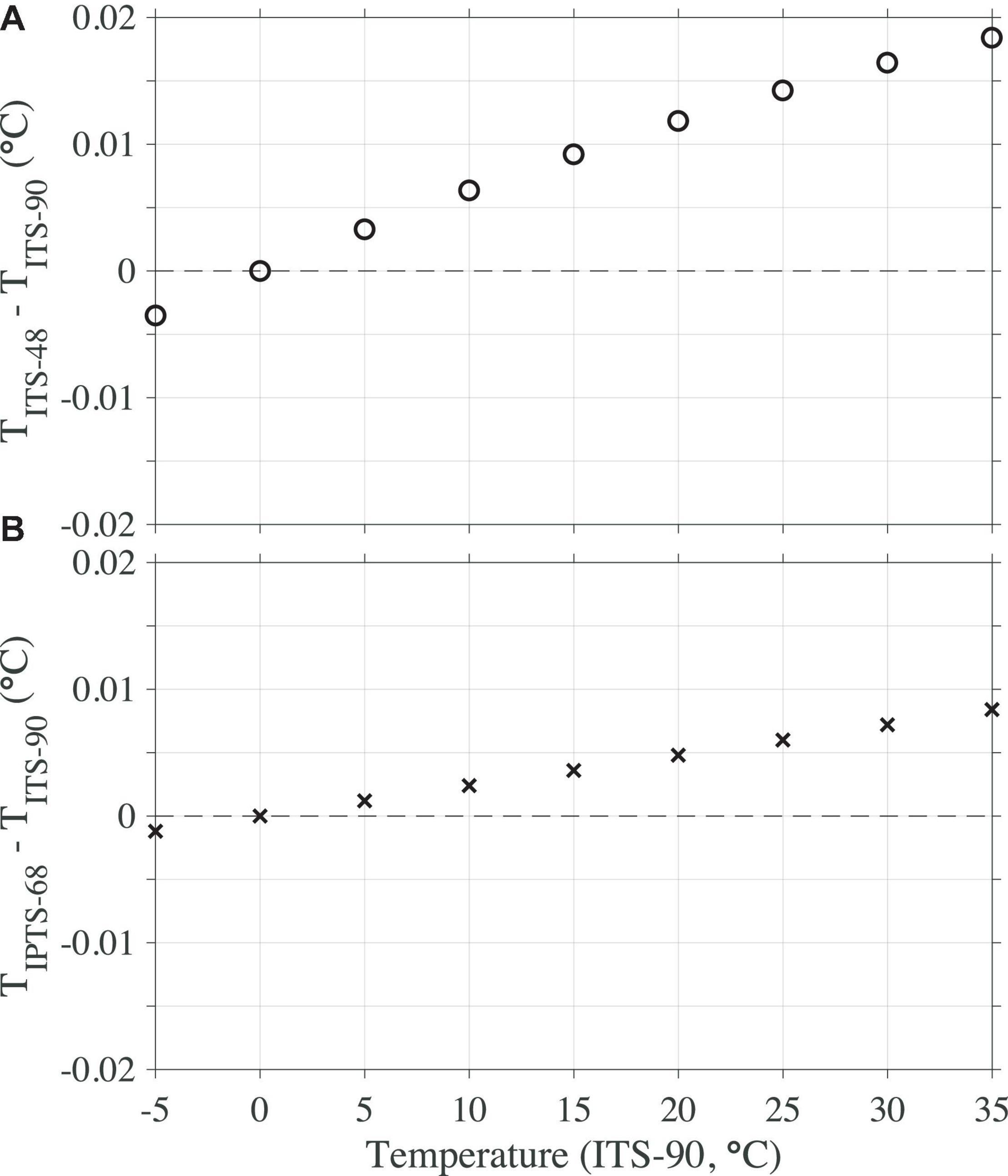
Figure 2. Comparison of water temperature at different temperature scales: ITS-48, IPTS-68, and ITS-90. (A) The differences between ITS-48 and ITS-90 against ITS-90. (B) The differences between IPTS-68 and ITS-90 against ITS-90. Water temperatures on ITS-48 or IPTS-68 can be converted to ITS-90 using the TEOS-10 functions of “gsw_t90_from_t48” and “gsw_t90_from_t68,” respectively (IOC et al., 2010).

The Practical Salinity (S_P, unitless) on the Practical Salinity Scale of 1978 (PSS-78) is recommended for reporting oceanographic observations (Krause et al., 1981; UNESCO, 1981, 1983). The practical salinity value is calculated from an equation involving the ratio of the electrical conductivity of a seawater sample to that of a standard potassium chloride (KCl) solution: a standard seawater sample with a S_P of 35 at 15°C (IPTS-68) and one atmospheric pressure would have the same conductivity ratio as a KCl solution containing 32.4356 g of KCl in a 1 kg mass of solution (UNESCO, 1981). The Absolute Salinity (S_A, unit: g/kg), which provides a thermodynamically consistent description of seawater properties (IOC et al., 2010), is generally calculated from S_P and composition anomalies, as direct estimates of S_A require the density of a sample to be measured under controlled laboratory conditions using a vibrating-tube densitometer (Wright et al., 2011). Absolute salinity is discussed further in the Supplementary Material.

For replicate measurements from the same Niskin bottle, it is recommended to report the median value rather than the mean value as used in the WOCE Exchange format of Swift and Diggs (2008). As mentioned previously, the use of “content” (i.e., per kg-seawater), instead of “concentration” (i.e., per liter) is recommended. Additionally, the use of moles requires that the molecular formula of the substance is clearly defined, e.g., use of “moles of oxygen” must make clear that moles of O₂ rather than moles of O is the intended understanding. Reporting a measured quantity as a content, even when the seawater quantity is measured out volumetrically, requires a knowledge of the seawater density, which can be calculated using the salinity and “measurement temperature” with the GSW_Sys tool (see section “Excel Tool for TEOS-10 Calculations”), then use of Eq. 3:

$\mathrm{Variable}(\mathrm{per}\mathrm{kg}\mathrm{SW})=\mathrm{Variable}(\mathrm{per}\mathrm{L})/\mathrm{Density}(\mathrm{kg}\mathrm{L}{}^{-1})(3)$

This “measurement temperature” should be the temperature of the seawater sample when the aliquot of the seawater sample to be analyzed was measured out by volume, not the in situ temperature. For example, for coulometer-based total dissolved inorganic carbon content (DIC) analysis, the temperature of the seawater sample in the pipette (i.e., at the point where the subsample’s volume is measured out) should be used. For oxygen measurements, the “measurement temperature” should be that when the sample is drawn from the Niskin bottle, as the “fixing” of the samples for Winkler titration takes place immediately after this. In cases where the fixing temperature is not available for oxygen samples, the in situ temperature should be used, assuming the sample is fixed shortly after collection. For nutrients, the “measurement temperature” should be that at which the standard solutions are prepared and the samples are measured (generally the lab temperature), as this is the temperature at which they are determined.

There are four commonly used pH scales in oceanographic research: the seawater scale (SWS), the “total” hydrogen ion content scale, or Total Scale (T), the “free” hydrogen ion content scale (F), and the NBS scale (NBS or NIST) (Dickson, 1984). The use of Total Scale (T) is recommended, but in any case, the scale that is used should be reported along with the measurement. Conversion of pH values from one scale to another can be done using the CO2SYS programs that will be described later. “pH_T_measured” (Table 1) is reserved for pH measurements from spectrophotometric methods (Byrne and Breland, 1989; Clayton and Byrne, 1993; Dickson, 1993). For pH measurements made from electrodes, “pH_T_measured (electrode)” should be used instead.

Discrete measurements of carbon dioxide (CO₂) in air that is in equilibrium with a seawater sample should be reported as carbon dioxide fugacity (fCO₂), instead of partial pressure (pCO₂). The mole fraction of CO₂ in a dry gas sample (xCO₂) is often measured by comparison with a calibration gas. This xCO₂ can then be converted to either partial pressure (pCO₂), or to fugacity (fCO₂), the latter of which accounts for the non-ideal behavior of CO₂ (Wanninkhof and Thoning, 1993; Pierrot et al., 2009; Figure 3). A newly developed tool to provide this conversion is discussed in section “fCO2_Calc Program to Calculate pCO₂ and fCO₂ from xCO₂.”

FIGURE 3

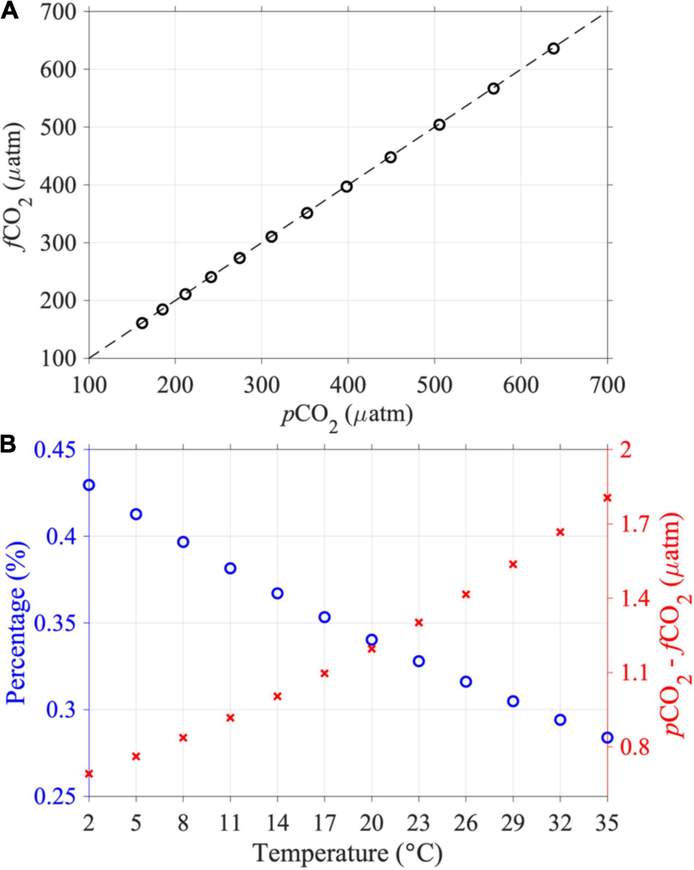
Figure 3. Plot of (A) the calculated carbon dioxide fugacity (fCO₂) against the calculated partial pressure (pCO₂), and (B) Relative differences (blue) between pCO₂ and fCO₂ against water temperature, and their absolute differences (red), based on a CO2SYS calculation using an imaginary seawater with the global average surface ocean temperature, salinity, DIC, and TA of 19.23°C, 34.87, 2020 μmol kg^–1, and 2306 μmol kg^–1, respectively (Jiang et al., 2015b), and using the recommended constants that are given in section “Recommended Dissociation Constants and Other Values for Carbon System Calculations” of the Supplementary Material.

As the values of pH, fCO₂, and [CO₃^2–] vary with temperature (and pressure) for a seawater sample that does not exchange substances (i.e., CO₂) with its surroundings (Figure 4), they must be accompanied with their corresponding report temperature. This should be the temperature of measurement instead of at a standardized temperature (such as 25°C) or the in situ temperature, to avoid potential ambiguity and conversion errors. Also, instead of using column headers such as fCO₂@25°C to indicate the temperature at which the parameter is measured, it is recommended that an extra column be used to denote this temperature. For example, TEMP_pH, TEMP_fCO2, and TEMP_Carbonate, refer to the temperature at which the pH_T_measured, fCO2_measured, and Carbonate_measured values are measured, respectively (Table 1). Because this data file is designed to document these values at the measurement condition (rather than the in situ condition), the pressure is assumed to be 1 atmosphere (0 dbar applied pressure).

FIGURE 4

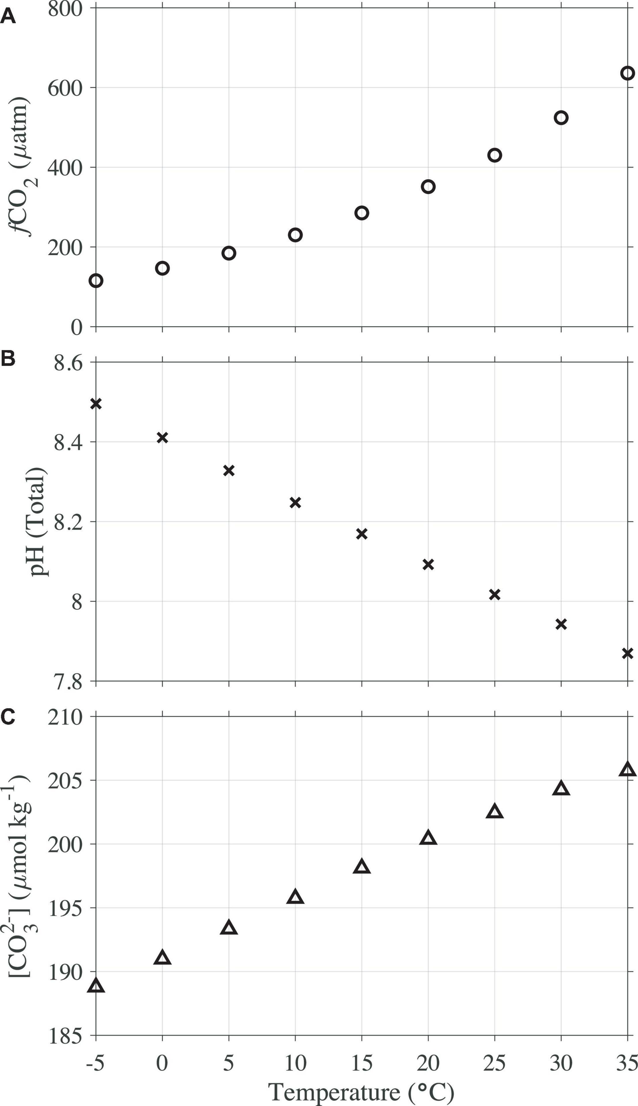
Figure 4. Temperature dependencies of (A) fugacity of carbon dioxide (fCO₂); (B) pH on Total Scale; and (C) carbonate ion content. The calculation is based on an imaginary seawater with the global average surface ocean temperature, salinity, DIC, and TA of 19.23°C, 34.87, 2020 μmol kg^–1, and 2306 μmol kg^–1, respectively (Jiang et al., 2015b) and using the recommended constants that are given in the section “Recommended Dissociation Constants and Other Values for Carbon System Calculations” of the Supplementary Material.

Chl_a is the heading to be used for discrete measurements of total chlorophyll a content from high-performance liquid chromatography (HPLC) (Table 1). Total chlorophyll a is the sum of divinyl chlorophyll a, monovinyl chlorophyll a, chlorophyllide a, chlorophyll a allomers, and chlorophyll a epimers. For continuous chlorophyll a readings, such as those from a fluorometer sensor, “Chl_a (sensor)” should be used.

Quality Control Flags

Data collected during the WOCE and the Global Ocean Ship-based Hydrographic Investigations Program (GO-SHIP) projects used WOCE primary level quality control (QC) flags (Joyce and Corry, 1994). There are three types of WOCE QC flags: one for Niskin bottles (Supplementary Table 3), one for discrete samples (Supplementary Table 4), and one for continuous measurements (Supplementary Table 5; Joyce and Corry, 1994). Similar to the IOC (2013) recommendation, the three types of QC flags are consolidated here into a single flagging scheme to avoid confusion (Table 2). This consolidated flagging scheme will be applicable to all types of chemical oceanographic data (discrete bottle, surface underway, and time-series).

TABLE 2

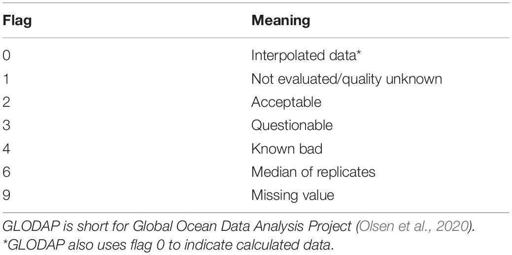
Table 2. Consolidated primary level quality control (QC) flags for chemical oceanographic data documentation.

Before consolidating the three WOCE QC flag tables, flags that were either obsolete or confusing were eliminated. For example, flags related to Gerard barrels were all removed because Gerard barrels are no longer used. To reduce confusion, Flag 9 is chosen to represent all missing values, as that is what the community has mostly been using. Flags 1, 5, and 9 previously could all mean “missing values”: 1 was for samples that were collected but not yet reported, 5 was for samples that were reported as “collected, but no value was available” (typically due to loss of a sample prior to, or during, measurement), and 9 was for samples that were not collected. Flag 0 is added because it is commonly used by the Global Ocean Data Analysis Project (GLODAP) community to indicate values that could have been measured but are somehow approximated (Olsen et al., 2020), either by vertical interpolations applied to temperature, salinity, dissolved oxygen, and nutrients, or through seawater CO₂ chemistry calculations for some carbonate parameters (e.g., DIC, TA, and pH). Note that Flag 0 is mainly reserved for data products and should not be used for data submission purposes, unless interpolated or calculated values are included in the data file.

It is recommended that only numerical QC flags be used, and that only one flag be placed in any QC field; otherwise, an entire column could be treated as text strings by some QC and plotting programs. For example, if a value is the median of several replicate measurements, the QC flag of “6” should be used, instead of using both “2” and “6” (Table 2). Additionally, the use of one QC flag column for several variables is discouraged. For example, a single “Nutrient_Flag” column should not be used for multiple columns of nutrients measurements (e.g., Nitrate, Nitrite, Ammonium, Phosphate, and Silicate). Likewise, missing value indicators should not be used in a QC flag column. If a data column has a missing value denoted as −999, the value “9” (the flag indicating missing value) should be placed in its corresponding QC flag column, rather than a missing value indicator, e.g., −999.

In addition, the GLODAP community has been using secondary level QC flags (Table 3). These flags are often documented in a separate column with a suffix of “_QC”, instead of “_FLAG” as is commonly used for primary level QC flags. These secondary level QC flags are presented here to give readers a complete picture of the QC flag scheme among the chemical oceanographic community that processes discrete bottle-based observations. Nevertheless, they are exclusive to data products like GLODAPv2 and should not be present in any submitted data file.

TABLE 3

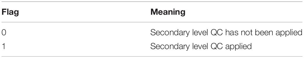
Table 3. Secondary level quality control (QC) flags for chemical oceanographic data product development, as used by GLODAPv2 (Olsen et al., 2016) – these should not be used for cruise data submission.

Missing Value Indicators

The WOCE manual recommends that “−9” be used in places where data are missing (Joyce and Corry, 1994). However, the most commonly used missing value indicators have been “−999” and “−9999,” because “−9” is a viable number for some variables. On rare occasions, extremely large numbers are also used as missing value indicators. To be consistent, “−999” is recommended to indicate missing values for all chemical oceanographic data files. “Not a number” (NaN) can also be used for programs that handle them well (e.g., MATLAB and IGOR).

Tools to Calculate Certain Properties

This section presents newly developed and upgraded tools to calculate certain quantities for chemical oceanographic data files. It is recommended that for data sharing and data publication purposes, calculated values not be included in the files, or if they are it must be clearly indicated in the metadata that the quantities listed are calculated values and not measured ones. Exceptions include the commonly accepted parameters: depth as calculated from hydrostatic pressure, salinity as calculated from conductivity and temperature, and fCO₂ as calculated from xCO₂.

Excel Tool for TEOS-10 Calculations

A newly developed Excel program (GSW_Sys_v1.0.xlsm)¹ uses the International Thermodynamic Equation of Seawater – 2010 (TEOS-10) to calculate depth (unit: meter) [or pressure (unit: dbar), depending on the input], Absolute Salinity (S_A, unit: g/kg), Conservative Temperature (Θ, unit: degree Celsius), potential temperature (θ, unit: degree Celsius), and potential density anomaly (σ_θ, unit: kg m^–3) from input of location (latitude and longitude), depth or pressure, practical salinity, and temperature. The name GSW derives from the Gibbs SeaWater (GSW) oceanographic toolbox that was developed by McDougall and Barker (2011). The Excel program also calculates apparent oxygen utilization (AOU) and percent oxygen saturation using the expression in Garcia and Gordon (1992). This tool should be cited as Pierrot et al. (2021). For more information about TEOS-10, refer to section “TEOS-10” of the Supplementary Material.

fCO2_Calc Program to Calculate pCO₂ and fCO₂ From xCO₂

A newly developed fCO2_Calc program² is also presented to standardize the calculation of partial pressure of carbon dioxide (pCO₂) and fugacity of carbon dioxide (fCO₂) from molecular ratio (mole fraction) of carbon dioxide in dry air (xCO₂) measurements. fCO₂ at the temperature of equilibration is calculated according to Wanninkhof and Thoning (1993); Dickson et al. (2007), and Pierrot et al. (2009). Water vapor pressure inside the headspace (pH₂O) is calculated with the equation of Weiss and Price (1980).

Updated CO2SYS and Seacarb

The CO2SYS (Lewis and Wallace, 1998; Pierrot et al., 2006; van Heuven et al., 2011) and seacarb (Proye and Gattuso, 2003; Gattuso and Lavigne, 2009) programs have been widely used to calculate seawater CO₂ system parameters. The versions that are being released in this paper (Table 4) are updated to enable:

TABLE 4

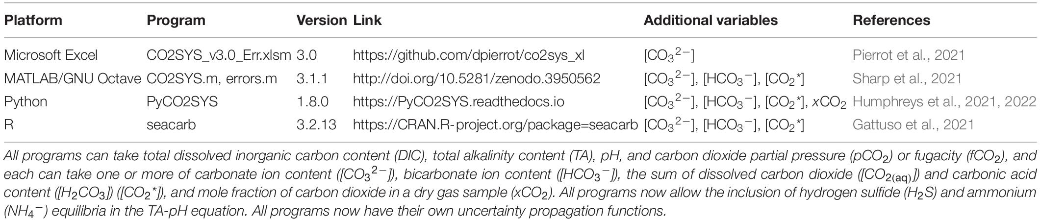
Table 4. Updated programs that are being released in this manuscript.

(a) The use of carbonate ion content ([CO₃^2–]), bicarbonate ion content ([HCO₃^–]), and aqueous CO₂ content ([CO₂*]) as input parameters,

(b) The inclusion of hydrogen sulfide (H₂S) and ammonium (NH₄^–) equilibria in the alkalinity-pH equation (Hagens and Middelburg, 2016; Xu et al., 2017) and,

(c) Full uncertainty propagation functions.

It is recommended that the programs be installed as described on their respective GitHub pages and/or online documentation (Table 4) to make sure the latest versions of the programs are used. It is likewise recommended that PyCO2SYS should be installed with pip as described in the documentation (see link in Table 4). PyCO2SYS has been described in detail by Humphreys et al. (2022). In the new Excel version of CO2SYS (Table 4; Pierrot et al., 2021), the pair of seawater CO₂ variables (columns J through O: DIC, TA, pCO₂, fCO₂, pH, and [CO₃^2–]) that will be used for the calculation can be indicated by clicking their corresponding header rows (Row #3), which will highlight the selected cells. The latest version of the R package seacarb (Gattuso et al., 2021) includes other functions useful for ocean acidification research, e.g., the ability to calculate pH from spectrophotometric measurements of absorbance ratios. “ScarFace” is a Shiny web application that has been developed to facilitate the use of seacarb via a user-friendly interface rather than with a command-line interface (Raitzsch and Gattuso, 2020).

Recommended dissociation constants for carbonic acid, bisulfate (HSO₄^–), and hydrofluoric acid (HF), as well as the equations to calculate total borate are presented in section “Recommended Dissociation Constants and Other Values for Carbon System Calculations” of the Supplementary Material. Note the recommended dissociation constants have been revised over time and may change in the future.

Sample Data Set

A column header example for discrete chemical oceanographic observations in CSV format named “33RO20200318_bottle.csv” is available in the Supplementary Material. The sequence of columns and parameters as shown in the example data file is recommended. When using the example file, columns can be deleted if there are no data to report, and new columns can be added if necessary (see Supplementary Table 1 for additional parameters). In case an abbreviation cannot be found in either Table 1 or Supplementary Table 1, the lead author (L-QJ, Liqing.Jiang@noaa.gov) should be notified so that new abbreviations can be added to the template in the future.

There are several additional recommendations for submitting data to a data center:

(1) Brief metadata about the data set should be recorded in rows above the column headers. Such rows should always start with the symbol “#.” Information related to any particular quality issues for a certain variable is especially recommended.

(2) Any columns without measurements (or composed entirely of missing values) should be deleted from the data file.

(3) Excel files should be converted to CSV before they are submitted to a permanent archive.

(4) It is also important to ensure the correct file extensions (e.g., CSV, XLSX, etc.) are used.

Naming Convention of Data Files

It is recommended that data files are named using (a) the EXPOCODE, and (b) observation type. For example, data files that are collected onboard NOAA Ship Ronald H. Brown (ICES code: 33RO) with a port departure date of July 23, 2018 (EXPOCODE: 33RO20180723) for discrete bottle measurements would have a name of “33RO20180723_bottle”. The use of spaces or hyphens in a file name is discouraged and the use of underscores is advised instead.

Best Practices Approach

The creation of this methodology document was motivated by feedback from users of NOAA/NCEI’s Ocean Carbon and Acidification Data System (OCADS)³ in terms of the WOCE Exchange format. It benefited from OCADS’ commitment to funnel the scientific expertise of the research community to the data management community.

The key to the success of this truly community effort was the assemblage of the group of experts who knew this topic well, and who would also be users of this document. The group was composed of (a) some of the most visionary researchers in this field, (b) experts on the measurement of these oceanographic parameters, (c) experts on oceanographic data quality control and product development, (d) experts on the related calculation tools, (e) experts on the new TEOS-10 system, and (f) experts on oceanographic data management.

To make the best decisions about these standards, we followed the steps below while writing this manuscript. Note it was very important for the coordinator to listen to the group’s wisdom, instead of trying to impose his/her own opinions into this process.

(a) All members were encouraged to express their own thoughts/opinions without any reservation.

(b) The coordinator (in this case, L-QJ) would try to make a decision, with help from experts in a particular aspect of the discussion.

(c) Then, the decision would be reevaluated by the group. Any undesirable decisions would be reversed in this “appeal-like” step.

(d) For tough decisions without a simple majority, we resorted to online polls.

Data Availability Statement

The original contributions presented in the study are included in the article/Supplementary Material, further inquiries can be directed to the corresponding author/s.

Author Contributions

L-QJ coordinated the effort and created the first draft of the manuscript. RW, RF, SA, DG, LB, BC, and L-QJ worked together to create the initial draft of the updated column headers. DP created these new programs with testing from L-QJ GSW_Sys_v1.0.xlsm, fCO2_Calc_v1.0.xlsm, and CO2Sys_v3.0_Err.xlsm. JDS created the MATLAB/GNU Octave version of the CO2SYS program (CO2SYS.m) and its error estimation program (errors.m), and worked closely with DP and MPH to ensure the MATLAB/GNU Octave, Excel, and Python versions of the CO2SYS programs produce consistent results. MPH created the Python version of CO2SYS (PyCO2SYS). J-PG and colleagues updated the R package seacarb. RW provided initial calculation equations for fugacity of carbon dioxide. DG provided equations and references for the calculation of apparent oxygen utilization and percent oxygen. All authors provided comments to the column headers and contributed to the writing of the manuscript.

Funding

Funding for L-QJ and AK was from NOAA Ocean Acidification Program (OAP, Project ID: 21047) and NOAA National Centers for Environmental Information (NCEI) through NOAA grant NA19NES4320002 [Cooperative Institute for Satellite Earth System Studies (CISESS)] at the University of Maryland/ESSIC. BT was in part supported by the Australia’s Integrated Marine Observing System (IMOS), enabled through the National Collaborative Research Infrastructure Strategy (NCRIS). AD was supported in part by the United States National Science Foundation. AV and FP were supported by BOCATS2 Project (PID2019-104279GB-C21/AEI/10.13039/501100011033) funded by the Spanish Research Agency and contributing to WATER:iOS CSIC interdisciplinary thematic platform. MH was partly funded by the European Union’s Horizon 2020 Research and Innovation Program under grant agreement N°821001 (SO-CHIC).

Conflict of Interest

The authors declare that the research was conducted in the absence of any commercial or financial relationships that could be construed as a potential conflict of interest.

The reviewer JB declared a past co-authorship with several of the authors JK, TTa, and EB to the handling editor.

Publisher’s Note

All claims expressed in this article are solely those of the authors and do not necessarily represent those of their affiliated organizations, or those of the publisher, the editors and the reviewers. Any product that may be evaluated in this article, or claim that may be made by its manufacturer, is not guaranteed or endorsed by the publisher.

Acknowledgments

The column headers for discrete chemical oceanographic data are a refinement and update to the Exchange format of the World Ocean Circulation Experiment (WOCE) Hydrographic Program with updates and refinements by the Climate and Ocean-Variability, Predictability, and Change (CLIVAR) and the Carbon Hydrographic Data Office (CCHDO) of the Scripps Institution of Oceanography. We thank Dwight Gledhill (NOAA Ocean Acidification Program, Silver Spring, MD, United States) and Kim Yates (St. Petersburg Coastal and Marine Science Center, St. Petersburg, FL, United States) for reading a previous version of the manuscript and offering comments that helped improve the manuscript significantly, and James Orr (Laboratoire des Sciences du Climat et l’Environnement, France) for key contributions to the R package seacarb and for contributing to the discussion about the best equations to estimate boron-salinity ratio. We also thank Tim Boyer and Scott Cross (NOAA National Centers for Environmental Information, Silver Spring, MD, United States) for comments that helped improve the manuscript, and Sabine Mecking (University of Washington, Seattle, WA, United States) for the CTD photo in Figure 1. We are grateful to Trevor McDougall (University of New South Wales, Australia) who pointed us in the right direction in the creation of the GSW_Sys tool. The paragraph about chlorophyll a data documentation benefited from the discussion with Crystal S. Thomas (National Aeronautics and Space Administration, Goddard Space Flight Center, Greenbelt, MD, United States). L-QJ thank the users of NOAA/NCEI’s Ocean Carbon and Acidification Data System (OCADS) for their feedback that motivated this work and contributed to many of these ideas. Any use of these standards and tools is for descriptive purposes only and does not imply endorsement by the U.S. Government. This is NOAA Pacific Marine Environmental Laboratory (PMEL) Contribution Number is 5244.

Supplementary Material

The Supplementary Material for this article can be found online at: https://www.frontiersin.org/articles/10.3389/fmars.2021.705638/full#supplementary-material

Footnotes

1. ^ https://github.com/dpierrot/GSW_Sys
2. ^ https://github.com/dpierrot/fCO2_Calc
3. ^ https://www.ncei.noaa.gov/access/ocean-carbon-data-system/

References

Brett, A., Leape, J., Abbott, M., Sakaguchi, H., Cao, L., Chand, K., et al. (2020). Ocean data need a sea change to help navigate the warming world. Nature 582, 181–183. doi: 10.1038/d41586-020-01668-z

PubMed Abstract | CrossRef Full Text | Google Scholar

Byrne, R. H., and Breland, J. A. (1989). High precision multiwavelength pH determinations in seawater using cresol red. Deep Sea Res. 36, 803–810.

Google Scholar

Byrne, R. H., and Yao, W. (2008). Procedures for measurement of carbonate ion concentrations in seawater by direct spectrophotometric observations of Pb(II) complexation. Mar. Chem. 112, 128–135. doi: 10.1016/j.marchem.2008.07.009

CrossRef Full Text | Google Scholar

Clayton, T. D., and Byrne, R. H. (1993). Spectrophotometric seawater pH measurements: total hydrogen ion concentration scale calibration of m-cresol purple and at-sea results. Deep Sea Res. 40, 2115–2129. doi: 10.1016/0967-0637(93)90048-8

CrossRef Full Text | Google Scholar

Comité International des Poids et Mesures. (1969). The international practical temperature scale of 1968. Metrologia 5, 35–44. doi: 10.1088/0026-1394/5/2/001

CrossRef Full Text | Google Scholar

Cvitas, T. (1996). Quantities describing compositions of mixtures. Metrologia 33, 35–39. doi: 10.1088/0026-1394/33/1/5

CrossRef Full Text | Google Scholar

Dickson, A. G. (1984). pH scales and proton-transfer reactions in saline media such as sea water. Geochim. Cosmochim. Acta 48, 2299–2308. doi: 10.1016/0016-7037(84)90225-4

CrossRef Full Text | Google Scholar

Dickson, A. G. (1993). The measurement of seawater pH. Mar. Chem. 44, 131–142.

Google Scholar

Dickson, A. G., Sabine, C. L., and Christian, J. R. (2007). Guide to best practices for ocean CO2 measurements. PICES Spec. Publ. 3:191.

Google Scholar

Garcia, H. E., and Gordon, L. I. (1992). Oxygen solubility in seawater: better fitting equations. Limnol. Oceanogr. 37, 1307–1312. doi: 10.4319/lo.1992.37.6.1307

CrossRef Full Text | Google Scholar

Gattuso, J.-P., and Lavigne, H. (2009). Technical note: approaches and software tools to investigate the impact of ocean acidification. Biogeosciences 6, 2121–2133.

Google Scholar

Gattuso, J.-P., Epitalon, J.-M., Lavigne, H., and Orr, J. (2021). seacarb: Seawater Carbonate Chemistry. R Package Version 3.2.16. Available online at: https://CRAN.R-project.org/package=seacarb (accessed October 18, 2021).

Google Scholar

Guenther, R., and Radebaugh, J. (2004). Understanding Metadata. Bethesda, MD: National Information Standards Organization (NISO) Press.

Google Scholar

Hagens, M., and Middelburg, J. J. (2016). Generalised expressions for the response of pH to changes in ocean chemistry. Geochim. Cosmochim. Acta 187, 334–349. doi: 10.1016/j.gca.2016.04.012

CrossRef Full Text | Google Scholar

Hassell, D., Gregory, J., Blower, J., Lawrence, B. N., and Taylor, K. E. (2017). A data model of the climate and forecast metadata conventions (CF-1.6) with a software implementation (cf-python v2.1). Geosci. Model Dev. 10, 4619–4646. doi: 10.5194/gmd-10-4619-2017

CrossRef Full Text | Google Scholar

Humphreys, M. P., Lewis, E. R., Sharp, J. D., and Pierrot, D. (2022). PyCO2SYS v1.8: marine carbonate system calculations in Python. Geosci. Model Dev. 15, 15–43, doi: 10.5194/gmd-15-15-2022

CrossRef Full Text | Google Scholar

Humphreys, M. P., Schiller, A. J., Sandborn, D. E., Gregor, L., Pierrot, D., van Heuven, S. M. A. C., et al. (2021). PyCO2SYS: marine carbonate system calculations in Python. Zenodo. doi: 10.5281/zenodo.5602840

CrossRef Full Text | Google Scholar

IOC (2013). Ocean Data Standards: Recommendation for a Quality Flag Scheme for the Exchange of Oceanographic and Marine Meteorological Data. IOC Manuals and Guides No. 54 (IOC/2013/MG/54-3), Vol. 3. UNESCO-IOC, Paris, 12.

Google Scholar

IOC, SCOR, and IAPSO (2010). The International Thermodynamic Equation of Seawater - 2010: Calculation and use of thermodynamic properties. Intergovernmental Oceanographic Commission, Manuals and Guides No. 56. Paris: UNESCO, 196.

Google Scholar

IUPAC (2014). Compendium of Chemical Terminology Gold Book. (Version 2.3.3). 1622. Available online at: https://goldbook.iupac.org/files/pdf/goldbook.pdf (accessed November, 2021).

Google Scholar

Jiang, L.-Q., O’Connor, S. A., Arzayus, K. M., and Parsons, A. R. (2015a). A metadata template for ocean acidification data. Earth Syst. Sci. Data 7, 117–125. doi: 10.5194/essd-7-117-2015

CrossRef Full Text | Google Scholar

Jiang, L.-Q., Feely, R. A., Carter, B., Greeley, D. J., Gledhill, D. K., and Arzayus, K. M. (2015b). Climatological distribution of aragonite saturation state in the global oceans. Glob. Biogeochem. Cycles 29, 1656–1673. doi: 10.1002/2015GB005198

CrossRef Full Text | Google Scholar

Joyce, T., and Corry, C. (1994). Chapter 4. Hydrographic Data Formats, in Requirements for WOCE Hydrographic Programme Data Reporting, WOCE Hydrographic Programme Office. Woods Hole, MA: Woods Hole Oceanographic Institution.

Google Scholar

Krause, D. C., Otto, L., Simpson, E. S. W., and Lal, D. (1981). Introduction of the practical salinity scale, 1978 and the new international equation of state of seawater, 1980. Deep Sea Res. 28A:1621. doi: 10.1016/0198-0149(81)90104-7

CrossRef Full Text | Google Scholar

Lewis, E., and Wallace, D. W. R. (1998). Program Developed for CO2 System Calculations, ORNL/CDIAC-105. Oak Ridge, TEN: Carbon Dioxide Information Analysis Center.

Google Scholar

Macintyre, F. (1976). Concentration scales: a plea for physico-chemical data. Mar. Chem. 4, 205–224. doi: 10.1016/0304-4203(76)90009-8

CrossRef Full Text | Google Scholar

McDougall, T. J., and Barker, P. M. (2011). Getting started with TEOS-10 and the Gibbs Seawater (GSW) Oceanographic Toolbox, SCOR/IAPSO WG127. 28 (accessed November, 2021).

Google Scholar

Olsen, A., Key, R. M., van Heuven, S., Lauvset, S. K., Velo, A., Lin, X., et al. (2016). The global ocean data analysis project version 2 (GLODAPv2) – an internally consistent data product for the world ocean. Earth Syst. Sci. Data 8, 297–323. doi: 10.5194/essd-8-297-2016

CrossRef Full Text | Google Scholar

Olsen, A., Lange, N., Key, R. M., Tanhua, T., Bittig, H. C., Kozyr, A., et al. (2020). An updated version of the global interior ocean biogeochemical data product, GLODAPv2.2020. Earth Syst. Sci. Data 12, 3653–3678. doi: 10.5194/essd-12-3653-2020

CrossRef Full Text | Google Scholar

Orr, J. C., Epitalon, J.-M., Dickson, A. G., and Gattuso, J.-P. (2018). Routine uncertainty propagation for the marine carbon dioxide system. Mar. Chem. 207, 84–107. doi: 10.1016/j.marchem.2018.10.006

CrossRef Full Text | Google Scholar

Orr, J. C., Epitaon, J.-M., and Gattuso, J.-P. (2015). Comparison of ten packages that compute ocean carbonate chemistry. Biogeosciences 12, 1483–1510.

Google Scholar

Pierrot, D., Epitalon, J.-M., Orr, J. C., Lewis, E., and Wallace, D. W. R. (2021). MS Excel Program Developed for CO2 System Calculations – Version 3.0 GitHub Repository. Available online at: https://github.com/dpierrot/co2sys_xl (accessed November, 2021).

Google Scholar

Pierrot, D., Lewis, E., and Wallace, D. W. R. (2006). MS Excel program Developed for CO2 System Calculations, ORNL/CDIAC-105a. Oak Ridge, TEN: Carbon Dioxide Information Analysis Center, doi: 10.3334/CDIAC/otg.CO2SYS_XLS_CDIAC105a

CrossRef Full Text | Google Scholar

Pierrot, D., Neill, C., Sullivan, K., Castle, R., Wanninkhof, R., Luger, H., et al. (2009). Recommendations for autonomous underway pCO2 measuring systems and data-reduction routines. Deep Sea Res. II 56, 512–522.

Google Scholar

Plomp, E. (2020). Going digital: persistent identifiers for research samples, resources and instruments. Data Sci. J. 19:46. doi: 10.5334/dsj-2020-046

CrossRef Full Text | Google Scholar

Preston-Thomas, H. (1990a). The international temperature scale of 1990 (ITS-90). Metrologia 27, 3–10. doi: 10.1088/0026-1394/27/1/002

CrossRef Full Text | Google Scholar

Preston-Thomas, H. (1990b). The international temperature scale of 1990 (ITS-90) - erratum. Metrologia 27:107. doi: 10.1088/0026-1394/27/2/010

CrossRef Full Text | Google Scholar

Proye, A., and Gattuso, J.-P. (2003). seacarb, an R Package to Calculate Parameters of the Seawater Carbonate System. Available online at: http://CRAN.R-project.org/package=seacarb

Google Scholar

Raitzsch, M., and Gattuso, J.-P. (2020). ScarFace – Seacarb Calculations With R Shiny User Interface (v1.3.0). Zenodo. doi: 10.5281/zenodo.4153455

CrossRef Full Text | Google Scholar

Riley, J. (2017). Understanding Metadata: What is Metadata, and What is it For?: A Primer. National Information Standards Organization. Available online at: https://groups.niso.org/apps/group_public/download.php/17446/Understanding%20Metadata.pdf (accessed November, 2021).

Google Scholar

Sharp, J. D., and Byrne, R. H. (2019). Carbonate ion concentrations in seawater: spectrophotometric determination at ambient temperatures and evaluation of propagated calculation uncertainties. Mar. Chem. 209, 70–80. doi: 10.1016/j.marchem.2018.12.001

CrossRef Full Text | Google Scholar

Sharp, J. D., Pierrot, D., Humphreys, M. P., Epitalon, J.-M., Orr, J. C., Lewis, E. R., et al. (2021). CO2SYSv3 for MATLAB. Zenodo. doi: 10.5281/zenodo.3950562

CrossRef Full Text | Google Scholar

Stimson, H. F. (1949). The international temperature scale of 1948. J. Res. NBS 42, 209–217. doi: 10.6028/jres.042.017

PubMed Abstract | CrossRef Full Text | Google Scholar

Stimson, H. F. (1961). The international practical temperature scale of 1948. J. Res. NBS 65A, 139–145.

Google Scholar

Swift, J. H., and Diggs, S. C. (2008). Description of WHP-Exchange Format for CTD/Hydrographic Data. Available online at: https://cchdo.github.io/hdo-assets/documentation/WHP_Exchange_Description.pdf (accessed November, 2021).

Google Scholar

Tanhua, T., McCurdy, A., Fischer, A., Appeltans, W., Bax, N., Currie, K., et al. (2019). What we have learned from the framework for ocean observing: evolution of the global ocean observing system. Front. Mar. Sci. 6:471. doi: 10.3389/fmars.2019.00471

CrossRef Full Text | Google Scholar

UNESCO (1981). The practical salinity scale 1978 and the international equation of state of seawater 1980. UNESCO Tech. Papers Mar. Sci. 36:25.

Google Scholar

UNESCO (1983). Algorithms for computation of fundamental properties of seawater. UNESCO Tech. Papers Mar. Sci. 44:53.

Google Scholar

van Heuven, S., Pierrot, D., Rae, J. W. B., Lewis, E., and Wallace, D. W. R. (2011). MATLAB Program Developed for CO2 System Calculations. ORNL/CDIAC-105b. Oak Ridge, TEN: Carbon dioxide information analysis center, doi: 10.3334/CDIAC/otg.CO2SYS_MATLAB_v1.1

CrossRef Full Text | Google Scholar

Wanninkhof, R., and Thoning, K. (1993). Measurement of fugacity of CO2 in surface water using continuous and discrete methods. Mar. Chem. 44, 189–204. doi: 10.1016/0304-4203(93)90202-y

CrossRef Full Text | Google Scholar

Weiss, R. F., and Price, B. A. (1980). Nitrous oxide solubility in water and seawater. Mar. Chem. 8, 347–359. doi: 10.1016/0304-4203(80)90024-9

CrossRef Full Text | Google Scholar

Wright, D. G., Pawlowicz, R., McDougall, T. J., Feistel, R., and Marion, G. M. (2011). Absolute salinity, “density salinity” and the reference-composition salinity scale: present and future use in the seawater standard TEOS-10. Ocean Sci. 7, 1–26. doi: 10.5194/os-7-1-2011

CrossRef Full Text | Google Scholar

Xu, Y.-Y., Pierrot, D., and Cai, W.-J. (2017). Ocean carbonate system computation for anoxic waters using an updated CO2SYS program. Mar. Chem. 195, 90–93. doi: 10.1016/j.marchem.2017.07.002

CrossRef Full Text | Google Scholar