ΔO2/N2′ as a New Tracer of Marine Net Community Production: Application and Evaluation in the Subarctic Northeast Pacific and Canadian Arctic Ocean

Introduction

Marine net community production (NCP) represents the difference between gross photosynthesis and community-wide respiration, exerting a first-order control on the ocean’s capacity to support upper trophic level biomass and sequester atmospheric carbon dioxide via the biological pump (Volk and Hoffert, 1985; Ware and Thomson, 2005). Accurately quantifying NCP is therefore important for understanding a variety of ecologically and economically important ocean processes, and for predicting climate-dependent shifts in marine biogeochemical cycles. Oceanic responses to climate change are likely to alter marine biological production (e.g., Moore et al., 2018), but our capacity to predict these changes is limited, in part, by poor data coverage. Multi-year NCP time-series are only available from a handful of deep ocean sites (Emerson, 2014), and many ship-based studies provide only sparse coverage in well-sampled ocean regions. New observational tools are thus required to facilitate NCP quantification on global scales and thereby enable predictions of its climate-related variability.

A common approach to estimating NCP involves quantification of the mixed layer O₂ mass balance, using O₂ measurements from ship-board surveys, moorings, profiling floats or gliders (e.g., Kaiser et al., 2005; Emerson and Stump, 2010; Bushinsky and Emerson, 2015; Palevsky and Nicholson, 2018). Since the O₂ saturation state is sensitive to both biological and physical processes, including temperature and salinity-dependent solubility effects and bubble injection, O₂ measurements alone are insufficient to accurately resolve NCP. To address this limitation, O₂ concentrations can be normalized to argon (Ar), a biologically inert gas with solubility properties that are virtually identical to O₂ (Craig and Hayward, 1987). The so-called “biological O₂ saturation anomaly,” ΔO₂/Ar (Eq. 1), defined by normalizing the seawater O₂/Ar ratio ([O₂/Ar]_sw) to the equilibrium ratio ([O₂/Ar]_eq), thus isolates the biological processes affecting O₂.

$$\mathrm{\Delta }{\text{O}}_2/\mathrm{Ar}=\left(\frac{{\left[{\text{O}}_2/\text{Ar}\right]}_{\text{SW}}}{{\left[{\text{O}}_2/\text{Ar}\right]}_{\text{eq}}}-1\right)\times 100\%(1)$$

In recent years, ship-based mass spectrometry has been employed to provide high-resolution coverage of NCP estimates from underway ΔO₂/Ar measurements (Kaiser et al., 2005; Tortell, 2005), yielding an improved understanding of the distribution of NCP (e.g., Kavanaugh et al., 2014; Eveleth et al., 2017; Juranek et al., 2019). However, the requirement for mass spectrometry generally limits deployments to research ships, while the expense of these instruments and the expertise required to deploy them at sea may be prohibitive to some research groups. Truly autonomous measurements on research vessels, volunteer observing ships (VOS), or in-situ platforms such as unmanned surface vehicles (USV) would significantly expand the global coverage of NCP estimates, helping to integrate these data with upper trophic level processes and observations of climatic variability across a range of scales.

Recent work has demonstrated that the seawater O₂/N₂ ratio, derived from simultaneous deployments of autonomous O₂ optode and gas tension device (GTD) sensors, may be used as an alternative to O₂/Ar measurements for high-resolution NCP estimates (Izett and Tortell, 2021). Observations from these instruments can be used to derive seawater nitrogen (N₂) concentrations (McNeil et al., 2005), and therefore calculate the biological O₂ saturation anomaly from in-situ O₂/N₂ measurements (i.e., ΔO₂/N₂, following Eq. 1). Relative to ΔO₂/Ar, however, ΔO₂/N₂ does not fully account for physical impacts on O₂, due to differences in the solubility properties of O₂ and N₂.

Izett and Tortell (2021) described an approach to correct for physical offsets between ΔO₂/N₂ and ΔO₂/Ar, using readily available environmental data and a modeling framework. The approach yields a new tracer, ΔO₂/N₂′ (denoted “N₂-prime”) which provides an analog for ΔO₂/Ar. In principle, ΔO₂/N₂′ holds significant promise as an NCP tracer under a range of oceanic conditions. To date, however, this approach has not been evaluated in the field, and no studies have reported NCP estimates derived from underway ΔO₂/N₂ or ΔO₂/N₂′. In this paper, we present an in-situ evaluation of ΔO ₂/N₂ and ΔO₂/N₂′ as NCP tracers, using observations from three research cruises in the Subarctic Northeast Pacific and Canadian Arctic Ocean. Our measurements allow us to compare ΔO₂/N₂, ΔO₂/N₂′ and ΔO₂/Ar over broad spatial scales and contrasting hydrographic regimes, and to evaluate the accuracy of the associated O₂/N₂-based NCP estimates. We demonstrate the strong utility of ΔO₂/N₂′ as an alternative to ΔO₂/Ar for autonomous NCP measurements across a range of oceanic environments, while also identifying conditions where uncorrected ΔO₂/N₂ is a useful NCP tracer. We evaluate potential errors in the estimation of NCP based on O₂/N₂ and provide recommendations for future deployments of optode/GTD systems as a tool for oceanic productivity measurements.

Materials and Methods

Deployments

We present data from three research cruises conducted during 2018 and 2019; two in the Subarctic NE Pacific (September 2018 and February 2019; Figure 1A) and one in the eastern and central Canadian Arctic Ocean, spanning the Labrador Sea (LS), Baffin Bay (BB) and the Canadian Arctic Archipelago (CAA; July–August 2019; Figure 1B). We denote the datasets as “NEP-summer,” “NEP-winter” and “Arctic-summer.” The two Subarctic Northeast Pacific (NEP) expeditions were conducted on board the CCGS J. P. Tully, as part of the Line P monitoring program (Department of Fisheries and Oceans Canada, cruise IDs 2018-040 and 2019-001, respectively), while the Arctic deployment was conducted on the CCGS Amundsen, as part of the ArcticNet program (Leg 2, cruise ID 1902).

FIGURE 1

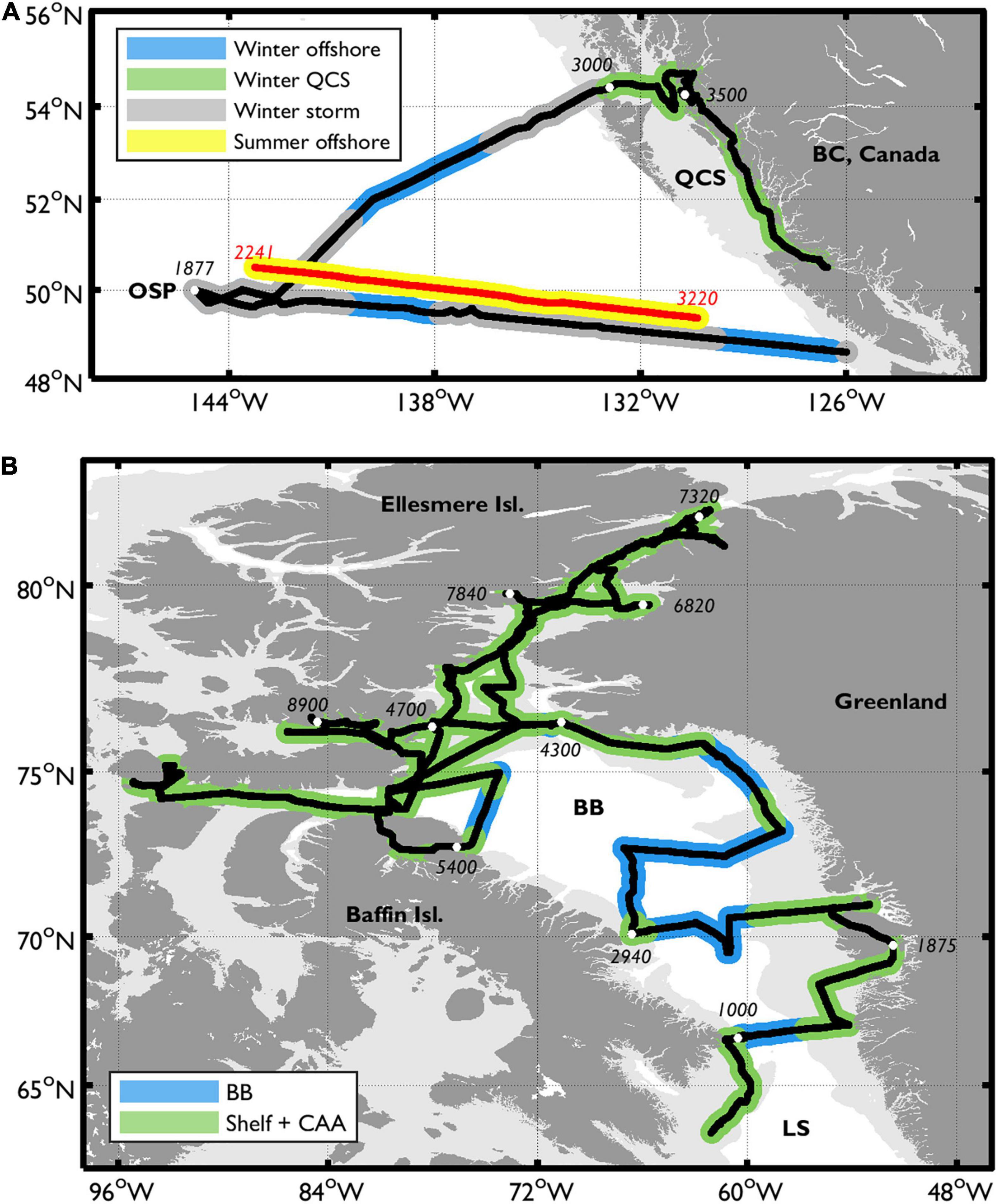
Figure 1. Survey ship tracks in the Subarctic NE Pacific (A), and the eastern Canadian Arctic (B) showing the locations where underway ΔO₂/Ar and ΔO₂/N₂ were compared. The approximate along-track distance (in km) is indicated with white markers for reference. In (A), black lines correspond with the NEP-winter track, while the red line represents the NEP-summer track, displaced north by 0.5-degrees for visibility. The thick gray lines in (A) represent regions that experienced elevated sea states and high surface winds. In both panels, pale gray shading represents the approximate continental shelf regions (<500 m bathymetry), and the sampling sub-regions are distinguished by color outlines around the cruise track lines. OSP, Ocean Station Papa; QCS, Queen Charlotte Sound; LS, Labrador Sea; BB, Baffin Bay; CAA, Canadian Arctic Archipelago.

On all cruises, gas and hydrographic observations were obtained using an underway optode/GTD, membrane inlet mass spectrometer (MIMS) and thermosalinograph. Seawater was pumped from nominal intake depths of ∼5 m (NEP cruises) and ∼7.5 m (Arctic cruise) to the ship’s laboratories and directed to the respective instruments. On the CCGS Tully, a progressive cavity pump (Moyno, 3L8CDQ) was used to supply water from the ship’s intake to the laboratory, while on the CCGS Amundsen, centrifugal magnetic drive pumps (thermosalinograph supply: March Pumps, BC-4C-MD; MIMS and optode/GTD laboratory: 1ST1H5A4-M01 NPE) were used. Pumped water was always obtained from within the mixed layer (Supplementary Figure 3). We omitted data corresponding with instances of instrument malfunction, and periods of seawater flow interruption resulting from ice blockages in the ship’s pumping system.

Underway ΔO₂/Ar and ΔO₂/N₂ Observations

Underway Gas Measurements and Data Processing

Measurements of O₂/Ar were made using a membrane inlet mass spectrometer (MIMS; Tortell, 2005). Briefly, seawater was circulated at a constant flow rate and temperature through a cuvette equipped with a 0.18 mm thick silicone membrane interfaced to the vacuum inlet of the mass spectrometer. Measurements of the mass-to-charge ratios at 32 (O₂) and 40 (Ar) AMU were obtained at approximately 20 s intervals. Water from an air-equilibrated standard bottle was introduced into the MIMS system every 45–90 minutes by automatically switching the inflow water source between the direct seawater supply and standard bottle. The standard consisted of ∼2 L of filtered seawater (<0.2 μm) gently bubbled using an aquarium air pump, and incubated at ambient sea surface temperature in an overflowing bucket. The seawater and air standard O₂/Ar ratios ([O₂/Ar]_sw and [O₂/Ar]_eq, respectively) were used to derive underway ΔO₂/Ar (following Eq. 1) by linearly interpolating between air standard measurements. On the NEP-summer cruise, final underway ΔO₂/Ar was obtained by calibrating the continuous measurements against discrete samples obtained from Rosette sampling (sample collection and processing details below). The underway data were linearly calibrated, with offsets between calibrated and uncalibrated signals ranging from ∼0 % (at ΔO₂/Ar values near equilibrium) to ∼3 % (at ΔO₂/Ar values of ∼10 %). No calibrations were performed on the NEP-winter or Arctic datasets.

Underway O₂ and N₂ data were derived from seawater measurements obtained using a custom-built optode/GTD system (Izett and Tortell, 2020), as described in the following section. The system recorded O₂ concentration (μmol L^–1) and total dissolved gas pressure (i.e., the sum of all gas partial pressures; TP, mbar) at ∼10 s intervals from an Aanderaa Data Instruments AS optode 4330 and Pro-Oceanus Systems Inc. mini-TDGP gas tension device, respectively. Debubbled seawater from the ship’s supply line was pumped rapidly and at constant flow rate past the instruments (∼2 L min⁻¹) to minimize the system residence time and hydrostatic pressure effects on the GTD measurements. A flow-through head (water residence time < 1 s) was installed on the face of the GTD to direct water onto the instrument’s Teflon membrane. The optode was submerged in a 0.25 L flow-through cell (residence time < 10 s) and oriented so that water flowed onto the sensing foil.

To improve the alignment between the optode/GTD, MIMS and hydrographic data (described below), and account for the slower response time of the GTD relative to the other gas sensors, we filtered the underway data (O₂, TP, ΔO₂/Ar, temperature, salinity) before deriving ΔO₂/N₂. All raw signals were low-pass filtered (frequency 0.5 min^–1) and subsequently median-binned into 2-min intervals. Following Hamme et al. (2015; their Eq. 2), we then applied a cumulative filter to all underway data (excluding GTD measurements) to replicate the rate of O₂ diffusion across the GTD membrane. We used a time-constant of 1/τ_GTD (where τ_GTD is the GTD’s temperature-dependent response time; ∼1–2 min, Izett and Tortell, 2020), extrapolated to the ambient seawater temperature. Finally, we adjusted for time offsets between sensors by manually aligning measurement peaks. Unless stated otherwise, all data presented below were processed in this manner.

Calculation of ΔO₂/N₂

Detailed handling and calibration procedures for O₂, N₂ and ΔO₂/N₂ are presented in the supporting material (Supplementary Material Section 1), and briefly summarized here. We corrected raw TP signals (TP^cor) for measurement bias (average offset < 1 mbar assessed as the difference between in-air GTD readings and atmospheric pressure) and for the effects of seawater warming between the intake and laboratory. Raw optode O₂ measurements were salinity-corrected (O₂^cor) following Uchida et al. (2008) and Bittig et al. (2018), and calibrated against discrete samples obtained from the outflow of the optode/GTD system or from Niskin bottles (details in the following section) to derive final O₂ concentrations (O₂^cal). Calibrated oxygen saturation $({\text{O}}_{2,\text{sat}}^{\text{cal}},\%)$ was derived by dividing O₂^cal by the O₂ solubility (Garcia and Gordon, 1992, 1993) calculated using ambient sea level and water vapor pressures (P_SLP and P_H2O obtained from reanalysis data products; see below) and sea surface salinity and temperature data from a thermosalinograph installed near the ship’s intake $\left(\mathrm{i}.\mathrm{e}.{\mathrm{O}}_{2,\text{sat}}^{\text{cal}}=\frac{{\text{O}}_2^{\text{cal}}}{{\text{O}}_{2,\text{eq}}\times \frac{{\text{P}}_{\text{SLP}}-{\text{P}}_{\text{H}2\text{O}}}{1013.25\mathrm{mbar}-{\text{P}}_{\mathrm{H2O}}}}\times 100\%\right)$.

We dervied the N₂ partial pressure (pN₂) following McNeil et al. (2005) by subtracting the partial pressures of O₂(obtained from ${\text{O}}_{2,\text{sat}}^{\text{cal}}$following Eq. 2), Ar and water vapor from TP^cor measurements (Eq. S7). The Ar saturation state (Ar_sat) and partial pressure were estimated from MIMS ΔO₂/Ar and optode ${\text{O}}_{2,\text{sat}}^{\text{cal}}$by re-arranging Eq. 1. The saturation state of all remaining gases (including Ar, when MIMS data were unavailable, and carbon dioxide) was assumed to be equivalent to N₂, following McNeil et al. (2005). The N₂ saturation level (N_2,sat), and resulting ΔO₂/N₂ (both %), were calculated following

$${\text{N}}_{2,\text{sat}}=\frac{{\text{pN}}_2}{\mathrm{\chi }{N}_2\times \left({\text{P}}_{\text{SLP}}-{\text{P}}_{\mathrm{H2O}}\right)}\times 100\%(2)$$

$$\mathrm{\Delta }{\text{O}}_2/{\text{N}}_2=\left(\frac{{\text{O}}_{2,\mathrm{sat}}^{\text{cal}}}{{\text{N}}_{2,\text{sat}}}-1\right)\times 100\%(3)$$

where χN₂ is the atmospheric dry mole fraction of N₂ (0.78084). As the saturation state of O₂, Ar or N₂ is equal to the ratio of observed concentration and equilibrium concentration at ambient temperature, salinity and P_SLP, Eq. 1 (for ΔO₂/Ar) and Eq. 3 (for ΔO₂/N₂) are equivalent. Individual gas supersaturation states (ΔO₂, ΔAr and ΔN₂) are calculated following the same convention as in Eq. 3 (i.e. ΔC = (C_sat/100-1) × 100 %). The equilibrium concentrations of N₂ and Ar were derived from the equations of Hamme and Emerson (2004) using temperature and salinity measurements made near the ship’s intake.

Underway Signal Calibration and Discrete Gas Samples

On each cruise, optode measurements were calibrated against discrete samples obtained from the outlet of the optode/GTD system. Discrete samples were analyzed by Winkler titration (automated colorimetric and potentiometric endpoint determinations during the NEP and Arctic cruises, respectively). We derived a best-fit linear regression between calibration samples and corresponding optode measurements (averaged within 2 min of sampling), and adjusted the calibrated O₂ for concentration differences between samples obtained from the flow-through seawater supply and mixed layer Niskin bottles (Eq. 3). While we did not observe any evidence of O₂ consumption in the ships’ seawater lines (Juranek et al., 2010), calibrating the optode signal against discrete samples from surface Niskin bottle sampling should correct for such potential sampling artifacts in subsequent studies. Since optode sensitivity drifts during storage, and in some cases during deployments (D’Asaro and McNeil, 2013; Bittig et al., 2018), we performed calibrations using discrete samples obtained over a range of hydrographic conditions and O₂ concentrations throughout the duration of each deployment. A single linear calibration was derived for each separate cruise dataset.

During the NEP-summer and Arctic cruises, underway N_2,sat data were calibrated using discrete gas samples obtained from Niskin bottles fired within the mixed layer as close to the depth of the seawater intake as possible. Discrete N_2,sat was calculated using N₂/Ar ratios measured in the bottle samples and corresponding underway Ar_sat. We obtained broad coverage of discrete samples across the Arctic cruise track, but reduced coverage during NEP-summer, and no samples from NEP-winter. All samples were collected in a manner that avoided bubble contamination and were preserved with saturated mercuric chloride solution before analysis by mass spectrometry, following Emerson et al. (1999) (NEP-summer samples) and Kana et al. (1994) (Arctic samples). ΔO₂/Ar was also measured in the discrete NEP-summer samples for calibration of the underway MIMS data. While no calibrations of the underway ΔO₂/Ar data were performed on the NEP-winter or Arctic cruises, calibrations of N_2,sat based on discrete N₂/Ar measurements and underway MIMS- and optode-derived Ar_sat should make the comparison of ΔO₂/Ar and ΔO₂/N₂ intrinsically consistent.

Discrete gas samples for subsurface N₂/Ar analyses were also collected during the NEP-summer and Arctic cruises (Supplementary Figure 5). Samples were collected at various depths and analyzed as described above. Subsurface N₂/Ar data were used in calculating N₂′, as described below. Detailed discrete gas sampling and analysis procedures are presented in Supplementary Material Section 1.3.

In discussing our results, we present calibrated data and omit the “cal” and “cor” superscripts. Gases (O₂, Ar or N₂) are represented by their saturation anomalies (i.e.,ΔC = (C_sat/100−1)×100%) referenced at ambient P_SLP. We calculate offsets between ΔO ₂/A r and ΔO₂/N₂ in two different ways: (1) based on their absolute difference (i.e., ΔO ₂/A r – ΔO₂/N₂); and (2) by using the tracer ΔN₂/Ar (calculated following Eq. 3 convention), which is independent of the O₂ saturation state. Gas ratios (ΔO₂/Ar, ΔO₂/N_2, and ΔN₂/Ar) are not influenced by ambient P_SLP.

Ancillary Datasets

Continuous measurements of sea surface temperature (SST) and salinity were obtained from a thermosalinograph installed near the ships’ seawater intakes (Sea-Bird SBE-21 and SBE-45/SBE-38 thermometer, on the CCGS Tully and CCGS Amundsen, respectively). Depth profiles of temperature and salinity were obtained from CTD casts (Sea-Bird SBE-911plus), and the mixed layer depth (MLD) was defined based on a 0.125 kg m^–3 density difference from the mean value in the upper 5 m (Thomson and Fine, 2003). We performed a two-dimensional spatial interpolation of MLD between CTD stations to estimate the MLD along the entire cruise tracks. Hydrographic data were provided by the Institute of Ocean Sciences (Department of Fisheries and Oceans Canada)¹ and the Amundsen Science group of U. Laval (Amundsen Science Data Collection, 2020a,b).

We obtained wind speed data at 10-m elevation from the CCMPv2 vector (Atlas et al., 2011), and NARR reanalysis (Mesinger et al., 2006) products for the NEP and Arctic, respectively. Gridded SST were from the NOAA High Resolution OI v2 dataset (Reynolds et al., 2007), and P_SLP and P_H2O data from the NCEP/NCAR reanalysis products (Kalnay et al., 1996). Sea ice fractional coverage was obtained from the AMSR-2 product (Spreen et al., 2008). The environmental data (excluding sea ice) were calibrated for our study regions using linear equations derived by comparing the gridded data with a multi-year ensemble of observations from moorings, buoys and ships in coastal and offshore waters (details in the Supplementary Material). The wind speed data were adjusted by < 1.2 m s^–1, on average, across both regions, while SST and P_SLP gridded data were adjusted by ∼0.2°C (NEP) and 0.6°C (Arctic) and 3 mbar, respectively. The average uncertainty in the adjusted wind speed, SST and SLP data, estimated as the mean deviation from ship-board measurements at the time of sampling was ∼3 m s^–1, 0.7°C and 2 mbar, respectively. We performed a nearest-neighbor interpolation of the adjusted gridded data to the cruise tracks at the time of data collection, and backward in time by 60 (NEP) to 90 (Arctic) days to determine the environmental histories of the sampling regions prior to the ship’s arrival (Supplementary Figure 3). The interpolated data were used to perform N₂′ calculations over the 60–90-day historical time period prior to our ship-based sampling. A longer (i.e., 90-day) time-record is required for ocean regions with longer mixed layer gas residence times.

N₂′: Correcting N₂ for Solubility, Bubble and Mixing Effects

Following Izett and Tortell (2021), we derived the term N₂′ to reconcile physical differences in Ar and N₂ supersaturation (ΔAr and ΔN₂) resulting from differential solubility properties, air-sea exchange rates, bubble effects and vertical mixing and advection. Full details and evaluation of the model calculations are presented in the Izett and Tortell manuscript, while Matlab scripts with examples for performing N₂′ calculations are available in a Matlab O2N2 NCP Toolbox² (Izett, 2021).

Briefly, we calculated the expected Ar and N₂ supersaturation difference (ΔN₂^mod – ΔAr^mod) at the time of our measurements using a simple one-dimensional model forced with gridded environmental data over one O₂ re-equilibration timescale prior to the ship-board observations (T_O2; see below). The model evaluates the mixed layer (ML) evolution of gas C (N₂ or Ar) following:

$$\frac{\text{d}\left(\text{C}\times \text{MLD}\right)}{\text{dt}}={\text{F}}_{\text{d}}+{\text{F}}_{\text{C}}+{\text{F}}_{\text{P}}+\frac{{\text{C}}_{\text{deep}}-\text{C}}{\text{dZ}}\times {\text{k}}_Z(4)$$

The first three terms on the right represent the air-to-sea flux via diffusive (F_d), and bubble-mediated (F_C + F_P; denoting fully collapsing and partially dissolving bubbles) processes, and the last term represents the vertical mixing flux. We used the model of Liang et al. (2013) to calculate the air-sea exchange terms in ice-free waters, and that of Butterworth and Miller (2016) to determine the total air-sea flux (F_C and F_P not explicitly parameterized) in partially ice-covered waters. The term $\frac{{\text{C}}_{\text{deep}}-\text{C}}{\text{dZ}}$ (mmol m^–4) represents the vertical gradient of Ar or N₂ between the surface and a given depth below the mixed layer (dZ, equal to the thickness of the pycnocline, as described in Izett and Tortell, 2021; their Figure 1). The κ_Z term (m² d^–1) is the vertical mixing rate. Subsurface Ar (Ar_deep) was set to the equilibrium concentration at subsurface temperature and salinity conditions derived by interpolating CTD measurements along the cruise track, and N_2,deep was derived from subsurface N₂/Ar data (i.e., ΔN₂/Ar_deep) and Ar_deep. In the NEP-summer and Arctic cruises, ΔN₂/Ar_deep was measured from N₂/Ar samples (Supplementary Figure 5 with further details in Supplementary Material Section 1.3), while archived data from Hamme et al. (2019) were used to characterize the deep gas conditions in NEP-winter (data provided at https://doi.org/10.1575/1912/bco-dmo.744563). κ_Z was derived from vertically resolved nitrous oxide (N₂O) measurements in the NEP (following Izett et al., 2018) and from NEMO circulation model simulations of the Arctic and N. Atlantic (NEMO model simulations described in Castro de la Guardia et al., 2019). In performing the N₂′ calculations, we subdivided our survey regions into smaller zones, which are described below. Mean ΔN₂/Ar_deep and κ_Z values were applied in each of these sub-regions (Supplementary Table 1), except in the Arctic where we used along-track κ_Z values based on the NEMO model output. We evaluate the sensitivity of the N₂′ calculations to these parameterizations in the discussion.

We calculated T_O2, the O₂ re-equilibration time, as −ln(0.01) × MLD/(k_T + κ_Z/dZ) (where k_T is the combined diffusive and large bubble-induced O₂ gas transfer velocity), and evaluated the budget by setting starting ML gas concentrations to C_eq. The re-equilibration timescale is approximately fivefold larger than the ML O₂ residence time (τ_O2 = MLD/k_T; Supplementary Figure 3), in order to fully erase the initial conditions invoked in the N₂′ model calculations. We assumed a constant MLD based on interpolated values from CTD casts. As discussed in Izett and Tortell (2021), this assumption may be problematic during periods of significant MLD changes (e.g., spring and autumn), but the uncertainty incurred in N₂′ calculations remains small relative to other NCP errors. In each time step, we calculated C_eq from time-variable SST and P_SLP, and constant salinity (based on ship-board measurements). The modeled difference between Ar and N₂ supersaturation (ΔC^mod) at the time of our cruise observations was then subtracted from optode/GTD-derived ΔN₂ observations to obtain ΔN₂′. We subsequently calculated N₂′_,sat from ΔN₂′, and re-evaluated ΔO₂/N₂ (as ΔO₂/N₂′) following Eq. 3 convention.

$$\mathrm{\Delta }N{}_2{}^{\prime }=\mathrm{\Delta }{N}_2^{\text{obs}}-(\mathrm{\Delta }{N}_2^{\text{mod}}-\mathrm{\Delta }\text{A}{r}^{\text{mod}})(5)$$

Calculations of Net Community Production

We estimated NCP (mmol m^–2 d^–1) as the product of the biological O₂ saturation anomaly, the O₂ equilibrium concentration (at 1013.25 mbar), and the O₂ gas transfer velocity (k_O2, m d^–1).

$$\mathrm{NCP}={\mathrm{k}}_{\text{O}2}\times \left(\mathrm{\Delta }{\text{O}}_2/\text{C}\right)\times {\left[{\text{O}}_2\right]}_{\text{eq}}(6)$$

In this approach, C represents either Ar, N₂ or N₂′, and NCP is equivalent to the diffusive sea-air flux of biologically produced excess O₂ (Teeter et al., 2018). We used the diffusive gas transfer velocity parameterization from Liang et al. (2013) in the NEP, and that of Butterworth and Miller (2016) in the Arctic [i.e. ko₂ scaled to the fraction of ice-free water, f, as k_O2 = k_O2 × (1-f)] to derive historical k_O2 values from the wind-speed observations. Final k_O2 was obtained by weighting these values over a 30-day period, following Teeter et al. (2018). Adjusting the length of the weighting period to account for different ML O₂ residence times does not have a significant effect on k_O2. Examples of these calculations are provided in the O2N2 NCP toolbox at (see text footnote 2).

Below, we present NCP estimates calculated using the three different metrics of the biological O₂ saturation anomaly: ΔO₂/Ar-NCP, ΔO₂/N₂-NCP and ΔO₂/N₂′-NCP.

Results

Our combined observations provide broad spatial coverage across a variety of oceanographic regimes throughout the Subarctic NEP and Canadian Arctic. In these contrasting regions, various physical and biological controls are expected to differentially affect gas saturation anomalies. For this reason, our combined dataset allowed us to examine a range of conditions under which measurements of ΔO₂/N₂ or ΔO₂/N₂′ can be used for accurate NCP derivation.

In describing our results, we divided the cruise tracks into distinct sub-regions (Figure 1). In the NEP, we differentiate between offshore (>500 m water depth) and nearshore waters. We only present results from the offshore section of the return (eastward) transect of the NEP-summer cruise due to periodic instrument problems on the outbound leg. In the NEP winter cruise, sampling within the nearshore region occurred in the Queen Charlotte Sound (QCS; > 2,700 km along-track). In the Arctic, we identify nearshore waters as those occurring over the Baffin Bay continental shelf (all regions overlying the continental shelf < 6,000 km along-track; identified by light gray shading in Figure 1B) and in the Canadian Arctic Archipelago (CAA), and offshore waters of Baffin Bay (BB; excluding shelf regions < 6,000 km along-track).

Underway Signal Calibration

We observed a strong linear relationship between optode and Winkler-based O₂ concentrations (R² = 0.99 for each cruise), enabling calibration of the underway data with a root mean square error (RMSE) of < 0.75% (Figure 2A). The calibration samples were collected throughout the duration of each deployment over a wide range of hydrographic conditions and O₂ concentrations (bars in Figure 2A), such that the calibrated O₂ should be accurate for the conditions encountered on each cruise.

FIGURE 2

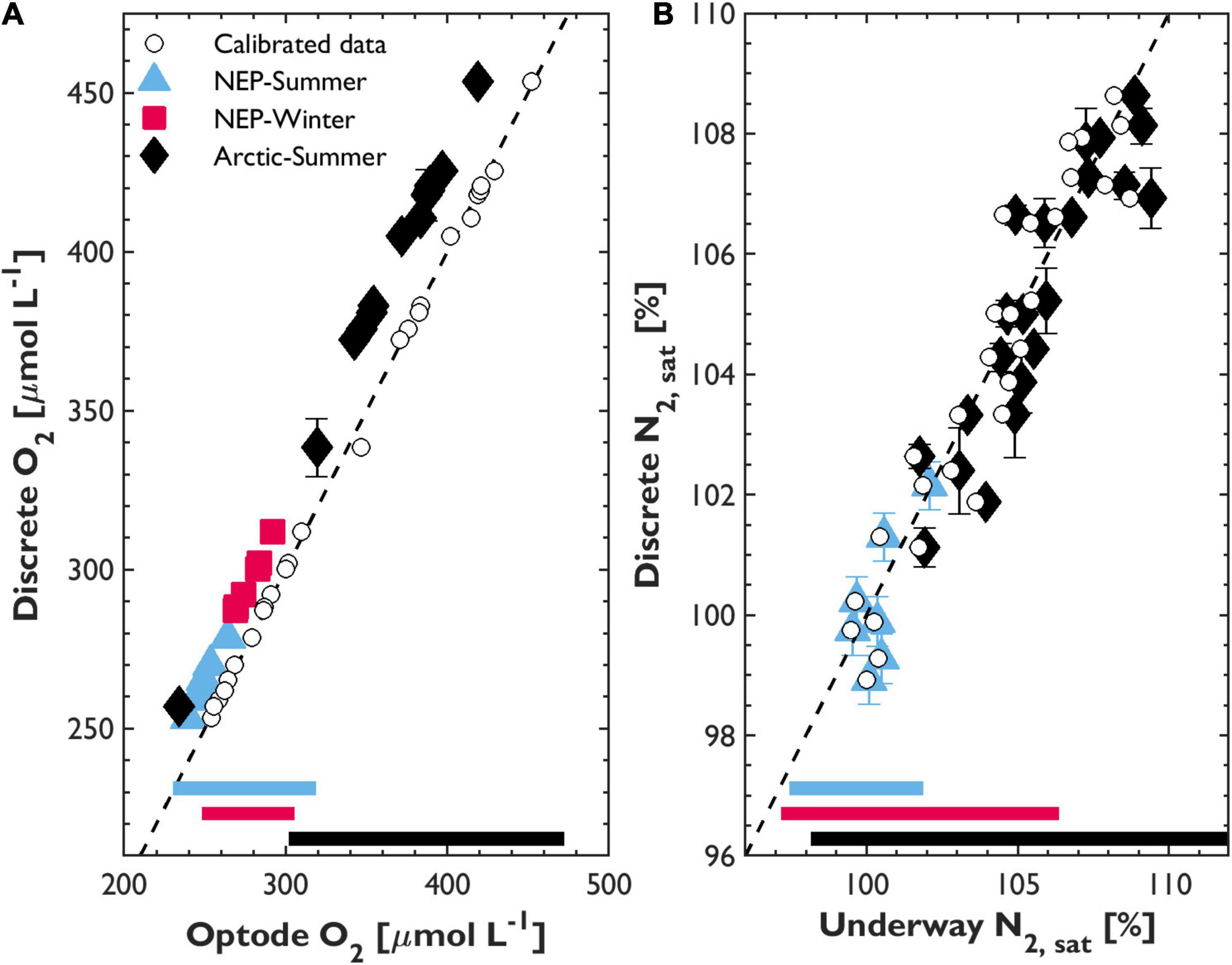
Figure 2. Calibration of underway O₂ (A) and N_2,sat (B) against discrete samples obtained from 2018 and 2019 Line P and Arctic cruises. Discrete O₂ samples were obtained from the seawater supply line, while N₂ samples were taken from Niskin bottles closed in the mixed layer. Underway sensor data (x-axis) represent the mean signal during a 2-min interval around the time of discrete sample collection. Error bars represent one standard deviation of the mean of duplicate discrete data; the standard deviation of the underway data is too small to resolve on the figure. The dashed line is the 1:1 line, and the bars at the bottom of each panel show the range of observed underway O₂ and N₂ on each cruise, excluding data during storm-impacted segments. The lowest Arctic O₂ calibration point (black diamond ∼260 μmol L^–1) represents an air-equilibrated standard obtained by bubbling seawater at ∼18°C before manually circulating through the optode/GTD system at the end of the Arctic cruise.

We also observed a strong linear relationship between underway and discrete N_2,sat (R² = 0.90, RMSE = 0.90% in the pooled NEP-summer and Arctic dataset; Figure 2B). Given the accuracy of O₂ (calibrated to < 1%) and TP (±0.1%, per Pro-Oceanus Systems Inc.) measurements, this calibration validates the underway N_2,sat data within an accuracy of ∼1%. Moreover, as discrete N₂ was derived using N₂/Ar ratios measured in the bottle samples and MIMS-based Ar_sat, this result suggests a similar accuracy for the underway ΔO₂/Ar data.

Since the NEP-summer and winter deployments used the same gas sensors, and we observed no drift in the GTD measurements over time (i.e., constant offset against atmospheric pressure), we applied the NEP-summer N₂ calibration to both datasets. Although the range of TP and N_2,sat conditions we encountered differed between the cruises (bars in Figure 2B), calibrations based on the NEP-summer, Arctic or pooled datasets resulted in derived ΔO₂/N₂ that varied by less than 0.4%. Across all cruises, the maximum difference between calibrated and uncalibrated N_2,sat was ∼2% at the highest saturation levels (mean ∼0.2%), suggesting that biases in ΔO₂/N₂ and derived NCP should be small even without N₂ calibrations. However, as the calculation of N_2,sat is sensitive to the degree of seawater warming between the ship’s intake and GTD (details in Supplementary Material Sections 2, 4), TP measurements should be made as close as possible to the ship’s seawater intake to minimize this source of error when calibration is not possible.

Surface Water Hydrography, Physical Forcing, and Gas Saturation Anomalies

We observed substantial spatial variability in surface hydrography (represented by sea surface salinity) across the study regions, and large temporal variability in physical forcing (wind speed, temperature changes and sea ice cover) prior to the cruise measurements. These factors contributed to large variations in mixed layer gas saturation states (ΔO₂/Ar, ΔO₂/N₂, ΔO₂, ΔAr, and ΔN₂). Figures 3–5 summarize underway observations as well as wind speed and SST change (ΔSST) over the mixed layer residence time of O₂, τ_O2. Supplementary Figures 2, 3 present the along-track ΔN₂ and ΔAr observations and environmental histories, respectively.

FIGURE 3

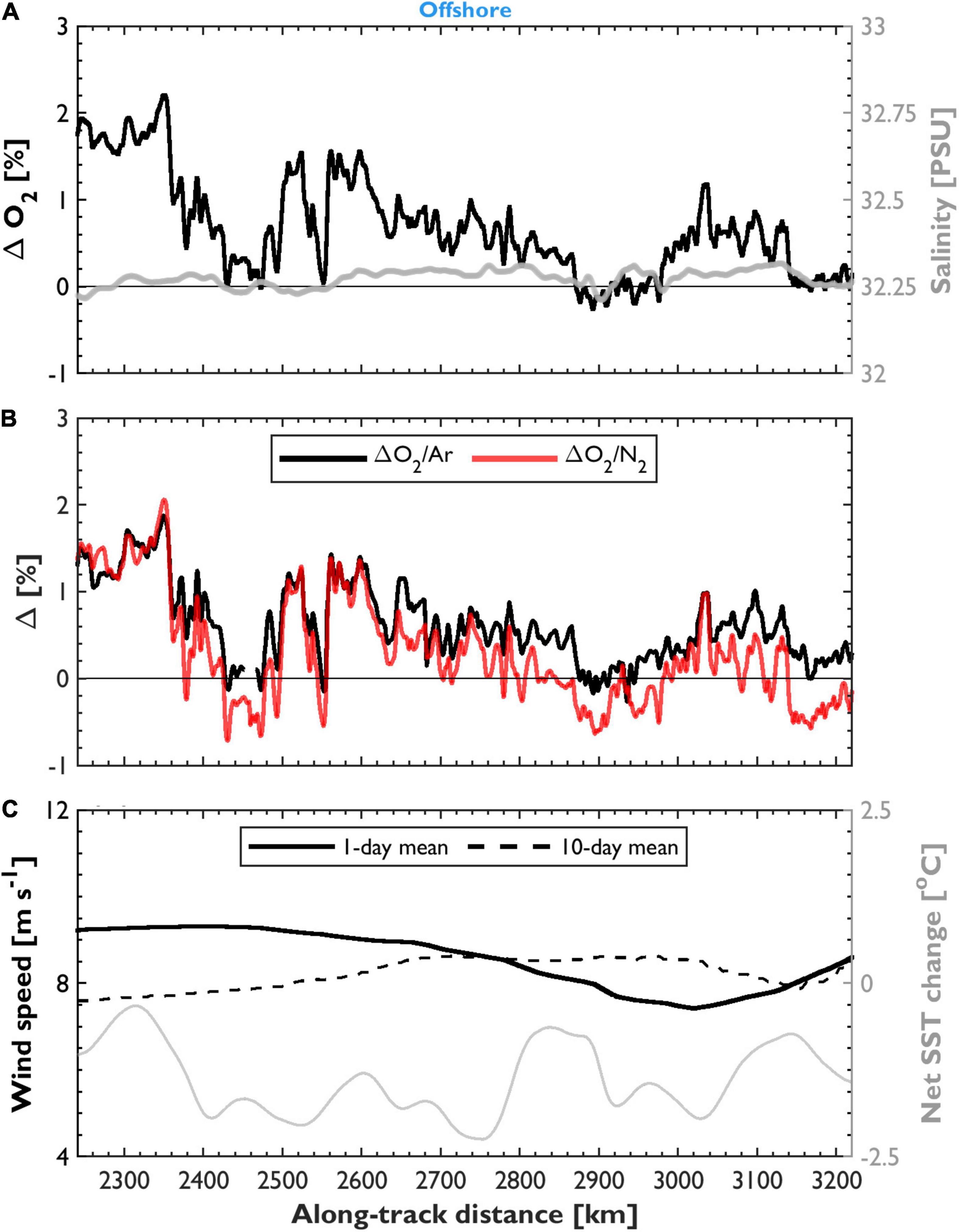
Figure 3. Spatial survey of ΔO₂ and salinity (A), ΔO₂/Ar and ΔO₂/N₂ (B), wind speed and net SST change (C) along the August 2018 Line P (NEP-summer) cruise track. Net ΔSST was calculated as the change in SST during one mixed layer τ_O2 prior to the cruise time, based on SST from NOAA reanalysis products. Wind speed data were taken from the ship’s sensors (1-day mean) and from the CCMP reanalysis product data (10-day mean). The transect was completed over ∼3 days.

FIGURE 4

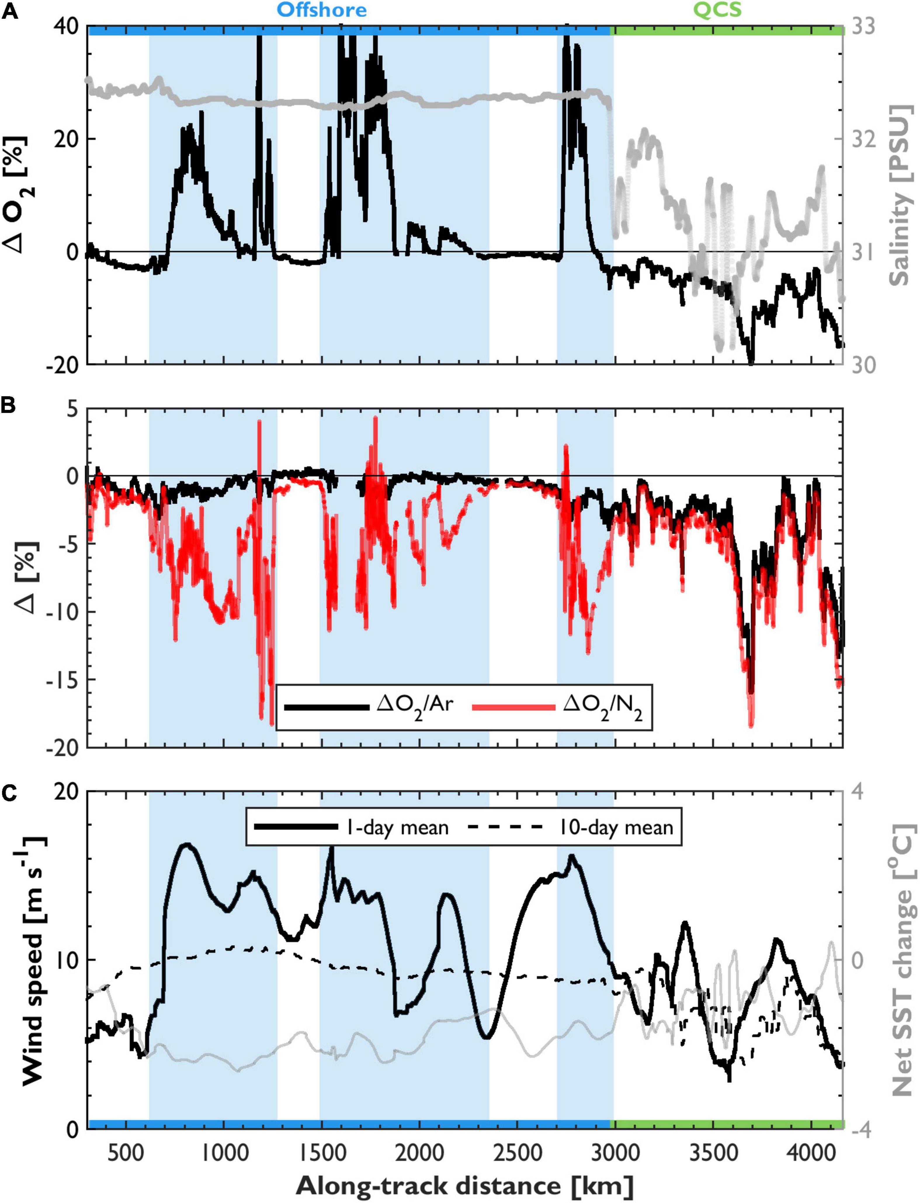
Figure 4. Spatial survey of ΔO₂ and salinity (A), ΔO₂/Ar and ΔO₂/N₂ (B), wind speed and net SST change (C) along the February 2019 Line P (NEP-winter) cruise track. The vertical light blue bars identify stormy sections of the transect. As described in the text, data from these regions were excluded from our analyses. The locations of the offshore and QCS regions are indicated by colored bars in (A,C), corresponding with those in Figure 1. The transect was completed over ∼15 days. Refer to Figure 3 caption for further details.

FIGURE 5

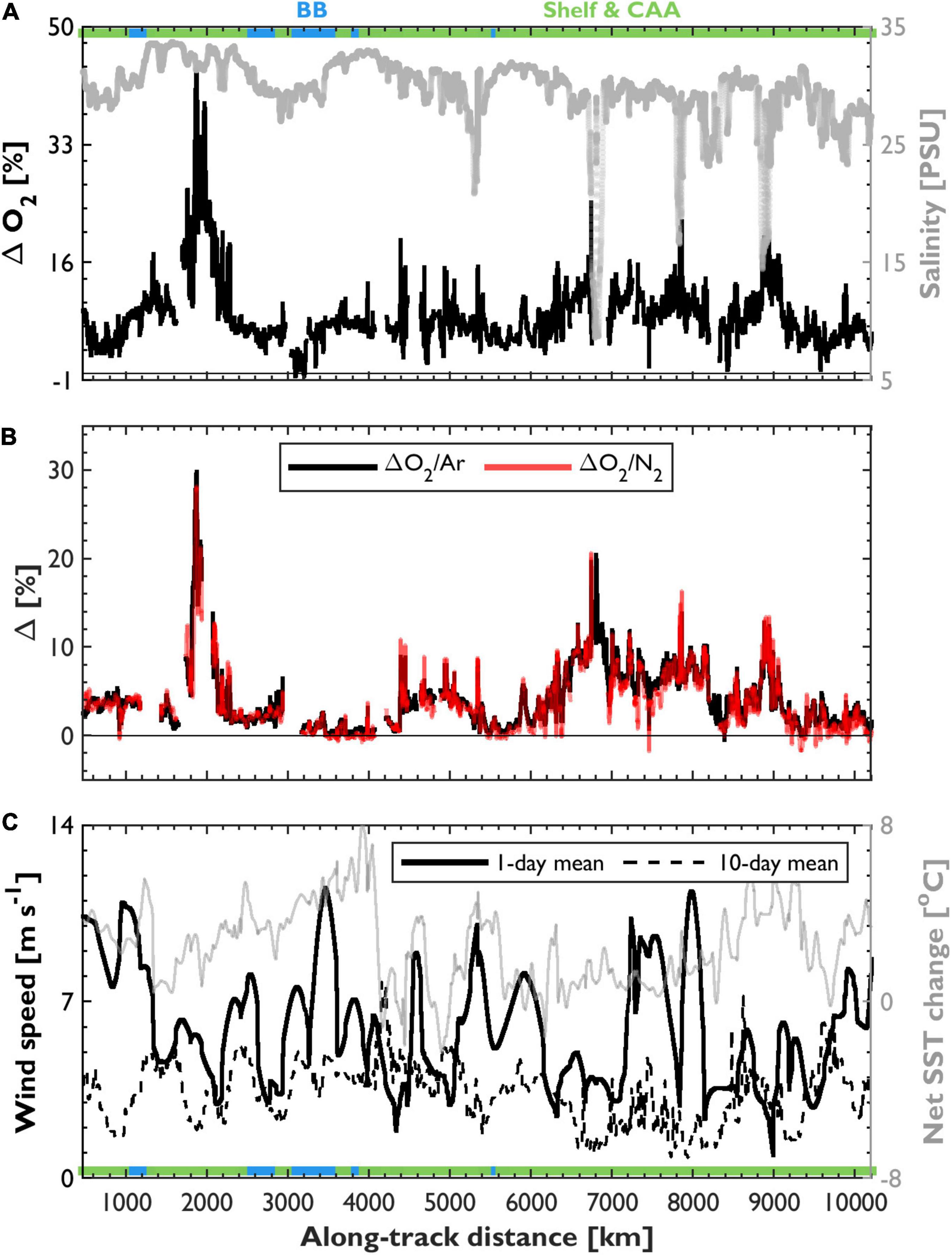
Figure 5. Spatial survey of ΔO₂ and salinity (A), ΔO₂/Ar and ΔO₂/N₂ (B), wind speed (NARR database) and net SST change (C) along the summer 2019 CCGS Amundsen (Arctic-summer) cruise track. The locations of the different regions are indicated by colored bars in (A,C). The transect was completed over ∼40 days. Refer to Figure 3 caption for further details.

Prior to our observations, wind speed and SST were highly variable in the NEP and Arctic, while Arctic sea ice coverage showed a declining trend (Supplementary Figure 3). On average, wind speeds during and prior to the NEP-winter cruise were higher and more variable than during the summer cruises (Figures 3C, 4C, 5C and Supplementary Figure 3). Several high-wind events (wind speed > 10 m s^–1) occurred near the time of our winter sampling, while wind speeds during and in the 60-days prior to the summer deployments were mostly below 10 m s^–1. Throughout most of the NEP-winter transect, surface waters experienced net cooling before the cruise, with the greatest cooling (∼3°C over τ_O2) observed in nearshore waters. The summertime NEP cruise also experienced net cooling of around 2°C over τ_O2. In contrast, warming was recorded over nearly the entire Arctic cruise track (ΔSST range −2–7°C; Figure 5C), with cooling observed in only several isolated regions.

Gas Observations in the Subarctic Northeast Pacific

Gas distributions and hydrographic properties differed between the summer and winter NEP cruises (Figures 3, 4 and Supplementary Figures 2, 3). Along the offshore NEP-summer track, we generally observed little spatial variability in all gases and hydrographic properties (Figure 3). During this summer cruise, ΔO₂, ΔAr and ΔN₂ were all within ∼2% of saturation, and ΔO₂/Ar and ΔO₂/N₂ strongly mirrored patterns in ΔO₂. ΔO₂/Ar typically exceeded ΔO₂/N₂ (i.e., ΔN₂ > ΔAr), and values ranged from ∼ −0.75 to 2%.

During NEP-winter, we observed extremely high ΔO₂, ΔAr and ΔN₂ (up to ∼40–50%; Figure 4A and Supplementary Figure 2B) corresponding with periods of very rough sea states and elevated wind speeds in offshore waters (blue shaded areas in Figure 4). In these stormy regions, ΔO₂/N₂ was highly erratic and exhibited some extremely low values (minimum −18%; Figure 4B), while ΔO₂/Ar showed little variability. Throughout the remainder of the winter transect, ΔO₂ was mostly undersaturated, and ΔAr and ΔN₂ were nearer to saturation (± 5%). ΔO₂/Ar almost always exceeded ΔO₂/N₂, and both tracers had an overall range of ∼−20–2%, strongly reflecting ΔO₂ variability. The lowest and most variable ΔO₂ values occurred in the nearshore QCS archipelago, corresponding with strong hydrographic fronts (Figure 4A). The largest offset between ΔO₂/Ar and ΔO₂/N₂ also occurred in the QCS region, where ΔN₂ was up to ∼2.5% higher than ΔAr.

Gas Observations in the Canadian Arctic

Gas saturation anomalies during the Arctic cruise contrasted those observed in the NEP (Figures 5A,B). Most notably, all gases (O₂, Ar, and N₂) were supersaturated and highly variable along most of the transect. ΔO₂/Ar typically exceeded ΔO₂/N₂ (ΔN₂ > ΔAr), and both were typically positive. As in the NEP, the distributions of ΔO ₂/A r and ΔO₂/N₂ followed patterns in ΔO₂, with the highest values (∼10–30%) occurring in the shelf and CAA regions (∼2,000 and >6,000 km along-track). Additional variability in ΔO₂, ΔO₂/Ar, and ΔO₂/N₂ corresponded with significant salinity features in the vicinity of freshwater sources from glacier run-off and river discharge throughout the shelf and CAA (e.g., sharp drops in salinity ∼5,400, 6,400, 6,800, 7,800, and 8,800 km; Figure 5A). ΔAr and ΔN₂ (Supplementary Figure 2C) were also higher and more variable in the Arctic than in the NEP (excluding storm-affected regions).

Comparison of Underway ΔO₂/Ar, ΔO₂/N₂, and ΔO₂/N₂′

The distribution of ΔO₂/Ar and ΔO₂/N₂ (excluding the storm-impacted sections of the NEP-winter) exhibited high spatial coherence on all cruises (Figures 3B, 4B, 5B, 6). The linear slope of the ΔO₂/Ar vs. ΔO₂/N₂ relationship was 1.08 ± 0.04 (R² = 0.96; uncertainty represents one-95% confidence interval around the least-squares slope) for the pooled dataset. These results demonstrate, to first order, the potential to use ΔO₂/N₂ as an NCP tracer in place of ΔO₂/Ar. In addition, ΔO₂/N₂ showed greater spatial coherence with ΔO₂/Ar than ΔO₂ alone (pooled dataset slope = 1.54 ± 0.03), supporting the continued normalization of O₂ measurements by a gas analog for NCP derivation.

FIGURE 6

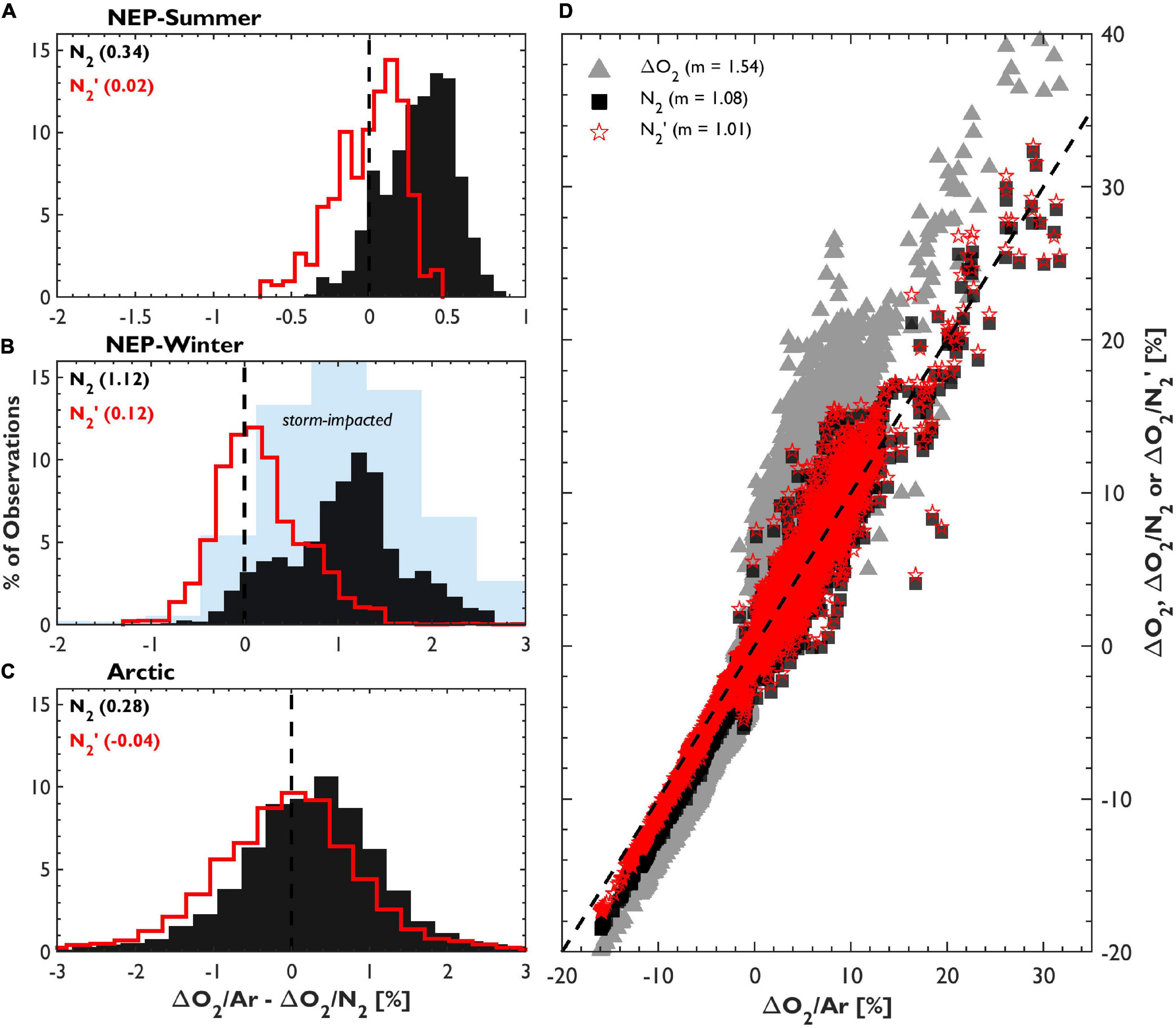
Figure 6. The relationship between ΔO₂/Ar and ΔO₂/N₂ or ΔO₂/N₂′ during the NEP-summer, NEP-winter and Arctic cruises. (A–C) Show the differences between ΔO₂/Ar and ΔO₂/N₂, before (black) and after (red outline) N₂′ corrections. The light blue shading in (B) represents storm-impacted data of the NEP-winter cruise. The numbers in the figure legends represent the median differences obtained from calculations using different N₂ terms. The x-axes in (A–C) have been truncated to exclude data representing less than 0.05% of observations. Direct correlations between ΔO₂/Ar and ΔO₂ (gray), ΔO₂/N₂ (black) and ΔO₂/N₂′ (red) data from all cruises (excluding storm-impacted data) are shown in (D). The linear slope value for each fit is included in the panel legend.

Despite the good agreement between ΔO₂/Ar and ΔO₂/N₂, small differences between the tracers remain. Figures 6A–C and Supplementary Figure 4 show the cruise-wide and regional offsets between ΔO₂/Ar and ΔO ₂/N ₂ before and after applying the N₂′ calculations. We observed median differences between ΔO₂/Ar and ΔO₂/N₂ of 0.3, 1.1, and 0.3% in the NEP-summer, -winter and Arctic datasets, respectively. Maximum deviations were up to ∼12% (excluding storm-impacted data with wind speeds exceeding ∼10 m s^–1), and the range of values was ∼18%. As discussed below, the most extreme values likely represent sampling artifacts rather than true differences between ΔAr and ΔN₂.

Applying the N₂′ corrections increased the alignment with ΔO₂/Ar on regional and sub-regional scales. Median offsets between ΔO₂/Ar and ΔO₂/N₂′ were reduced to approximately 0.02% (NEP-summer), 0.1% (NEP-winter) and −0.04% (Arctic). The largest reduction in the bias between tracers occurred during the winter NEP cruise, while throughout the Arctic, ΔO₂/N₂ and ΔO₂/N₂′ were more similar. Overall, the direct comparison between all pooled ΔO₂/Ar and ΔO₂/N₂′ observations had a linear regression slope not significantly different from unity (1.01 ± 0.03 with R² of 0.96).

Net Community Production Estimates

We did not compare ΔO₂/ Ar-, ΔO₂/N₂-, and ΔO₂/N₂′-based NCP values on a point-by-point basis, since results are influenced by the differential response times of the gas sensors. Rather, we compared NCP estimates after binning the respective datasets into 20-km intervals. Table 1 and Figure 7 summarize the derived NCP values by sub-region.

TABLE 1

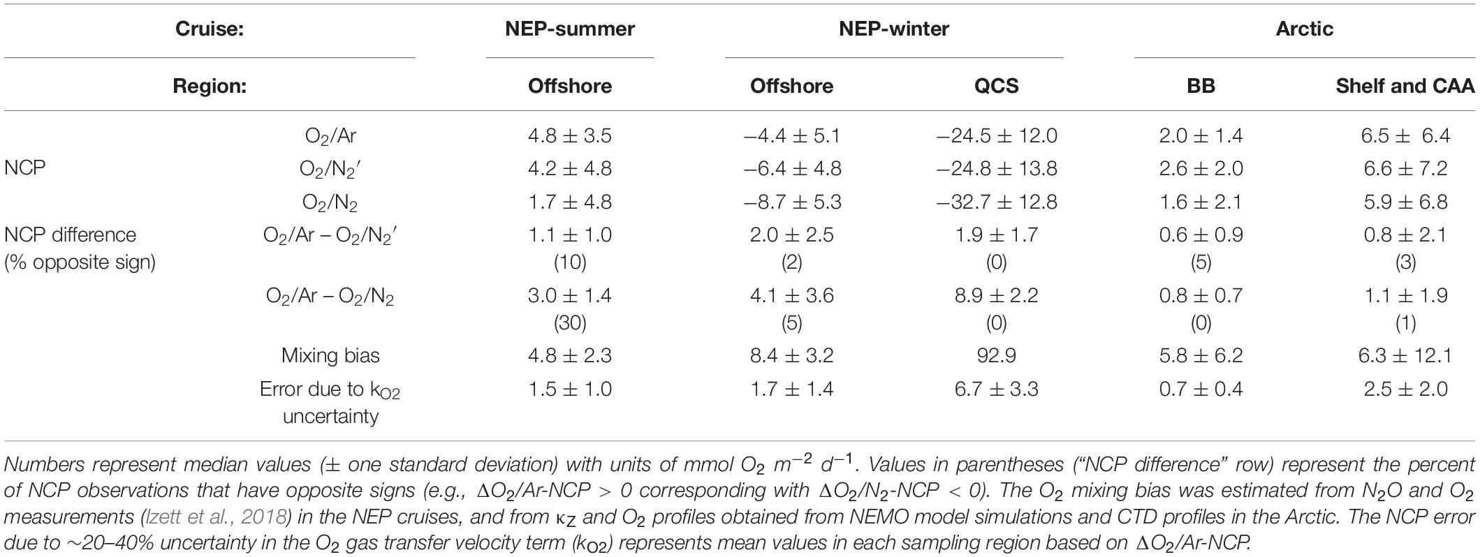
Table 1. Summary of NCP estimates, differences between NCP terms and other biases in NCP calculations during the 2018 and 2019 NEP-summer, NEP-winter and Arctic cruises.

FIGURE 7

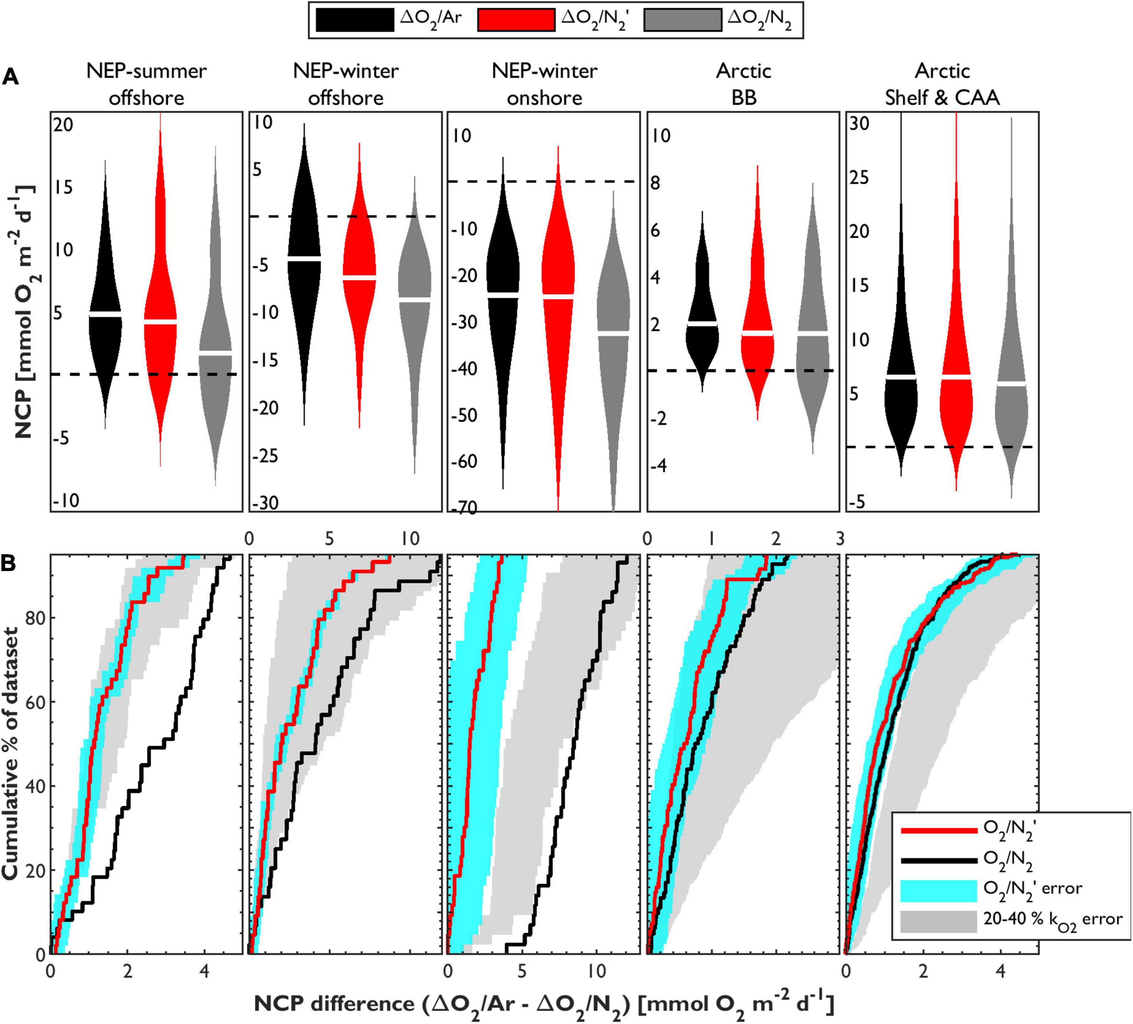
Figure 7. Comparison of NCP estimates derived from ΔO₂/Ar, ΔO₂/N₂ and ΔO₂/N_2’ measurements obtained during the 2018 and 2019 NEP-summer, NEP-winter and Arctic cruises. (A) Shows the distribution of NCP estimated using each biological O₂ saturation anomaly for each cruise and sub-region. NCP estimates were binned to 20-km intervals and have not been corrected for vertical mixing biases on surface O₂, which would influence all NCP estimates to the same extent. The white line represents median values for each distribution. (B) Shows the cumulative frequency distribution of biases in ΔO₂/N₂′- and ΔO₂/N₂-based NCP estimates relative to ΔO₂/Ar-NCP. Y-axis values represent the proportion of the dataset with NCP biases lower than a given x-axis value. The blue patches represent errors in ΔO₂/N₂′-NCP, assessed as the combined analytical uncertainty and sensitivity to the κ_Z and ΔN₂/Ar_deep terms. The gray patch represents NCP biases incurred by a 20–40% uncertainty in the O₂ gas transfer velocity (k_O2).

We observed the largest range of NCP values in the nearshore (QCS) waters of the Subarctic NE Pacific, and highest values (up to ∼30 mmol O₂ m^–2 d^–1) in the Arctic shelf and CAA. Derived values were mostly negative during NEP-winter, and predominantly positive in both summer cruises. The strong negative values in the QCS likely reflect biases from vertical mixing of low O₂ waters, rather than in situ heterotrophy. Whereas NCP estimates derived from uncorrected ΔO₂/N₂ showed a higher frequency of negative values compared with ΔO₂/Ar-derived NCP (15% of pooled dataset), application of N₂′ significantly reduced the frequency of negative values (to 4%) in all sub-regions. Our observations thus suggest that N CP estimated from ΔO₂/Ar and ΔO₂/N₂′ provided consistent representation of the metabolic state of surface waters on regional scales. Moreover, as shown in Figure 7B, N₂′ calculations reduced biases in derived NCP across the dataset. Indeed, ΔO₂/N₂′-NCP values calculated in each sub-region were generally closer to ΔO₂/Ar-based estimates, with median offsets < 2 mmol O₂ m^–2 d^–1, as compared to < 9 mmol O₂ m^–2 d^–1 for ΔO₂/N₂-NCP. In contrast to the NEP cruises, however, NCP estimates derived ΔO₂/N₂′ and ΔO₂/N₂ were nearly equivalent in parts of the Arctic (particularly in shelf and CAA waters), suggesting that N₂′ was less important for reducing NCP biases in this region during the time of our sampling.

Discussion

Uncertainty and Artifacts in Surface ΔO₂/N₂ Observations

A key result of this work is that ΔO₂/Ar and ΔO₂/N₂ show strong spatial coherence across all cruise transects, excluding regions in the Subarctic Pacific impacted by winter storms. Despite this overall agreement, important differences exist between these measurements, leading to ΔN₂/Ar disequilibria and offsets in derived NCP estimates. These can be attributed to physical processes, including solubility changes and bubble and mixing effects, which cause ΔAr and ΔN₂ to diverge, and to analytical or measurement uncertainty which must also be considered.

Bubble Entrainment During Elevated Sea States

The anomalous gas observations in parts of the offshore Subarctic NE Pacific winter data represent a limitation of the present application of O₂/N₂-based NCP estimates. Several lines of evidence suggest that the exceedingly high ΔO₂, ΔAr, and ΔN₂ and strongly negative ΔO₂/N₂ measured in the wintertime offshore Subarctic NEP (Figures 4A,B and Supplementary Figure 2B) reflect artifacts from bubble entrainment in the ship’s seawater supply during periods of elevated sea states. Following Vagle et al. (2010), application of the ideal gas law (n = (f×χ×p_SLP)/(R×SST))shows that dissolution of bubbles with an air-volume fraction (f) of only ∼4% is sufficient to yield the elevated ΔO₂, ΔAr, and ΔN₂ values observed during the cruise (up to ∼45%). In contrast, observed noble gas and N₂ supersaturation seldom exceed ∼6% in the subarctic ocean (Steiner et al., 2007; Emerson and Bushinsky, 2016; Hamme et al., 2019), even under extreme hurricane-force winds (wind speeds up to 57 m s⁻¹; D’Asaro and McNeil, 2008). Moreover, most air-sea exchange parameterizations predict bubble-induced supersaturation anomalies of O₂, N_2, and Ar of less than ∼6% at wind speeds below 20 m s^–1. Only extremely rapid warming (>10°C over several days) could yield such strong positive supersaturation anomalies of all three gases, but we observed net cooling before the winter cruise (Figure 4C). Finally, such anomalies do not reflect sampling artifacts in the optode/GTD system, since it was designed to successfully divert bubbles from the instrument interfaces (Izett and Tortell, 2020). We thus conclude that the anomalously high gas supersaturation values we observed during the NEP-winter cruise resulted from bubble dissolution in the ∼100 m of piping between the ship’s seawater intake and laboratory.

As O₂ and Ar have very similar solubility properties, the bubble effect on ΔO₂/Ar is small (but not entirely negligible for high rates of bubble dissolution). In contrast, the reduced solubility of N₂ relative to O₂ results in elevated N₂ sensitivity to bubble dissolution and a large negative ΔO₂/N₂ anomaly. Based on these observations, we suggest that O₂/N₂ measurements should not be used to calculate NCP when significant bubble dissolution in the ship’s underway sampling system is suspected. More generally, the set of criteria we used to discard ΔO₂/N₂ data (i.e., strongly negative ΔO₂/N₂ corresponding with ΔN₂ > ΔO₂ and both > ∼5%) should be applicable to many ocean regions that experience modest short-term temperature changes and minimal microbial N₂ production. Future work should, however, evaluate our criteria for other ships and ocean regions. For example, it is important to note that negative ΔO₂/N₂ does not imply poor data quality, per se. The nearshore waters of the NEP-winter cruise provide an example of negative ΔO₂/N₂ (Figure 4B) likely resulting from significant vertical fluxes of O₂-deplete water, rather than bubble entrainment artifacts. Observations should thus be considered in light of the environmental forcing histories prior to sampling, and of additional gas fluxes that may produce negative ΔO₂/N₂. Moreover, we note that elevated wind speeds alone may not be a strong criterion for identifying potentially biased data, since we encountered periodic u₁₀ exceeding 10 m s^–1 without excursions in the gas data during the Arctic cruise (Figure 5). Finally, our data quality criteria may not identify impacts of smaller bubble dissolution signatures, but such effects could be diagnosed by careful inspection of the underway data for differences in stochastic N₂ variability relative to O₂. Indeed, as the underway sampling suggests, the spatial and temporal variability of O₂ is typically much greater than that of N₂ or Ar (compare ΔO₂ in Figures 3A, 4A, 5A with ΔAr and ΔN₂ in Supplementary Figure 2). Overall, bubble artifacts can likely be reduced by installing the optode/GTD system closer to the seawater intake, thereby reducing the distance and time over which bubbles can dissolve. This issue should also be less important on larger ships which are less susceptible to rolling and pitching during elevated sea states, or on ships with deeper intakes where the chance of entraining air in the underway seawater system is reduced.

Additional Sources of Analytical Uncertainty

Outside of the storm-impacted sections, we observed median offsets between ΔO₂/Ar and ΔO₂/N₂ of less than ∼1.5% in all cruise regions. Given the calibrated accuracy of the underway O₂, N_2,sat and ΔO₂/Ar data, we believe that these median signals largely represent real physical differences between ΔO₂/Ar and ΔO₂/N₂. However, the full range of differences between ΔO₂/Ar and ΔO₂/N₂ extended from ∼−6 to 12%. This large range is attributable to some sources of measurement uncertainty and the sensitivity of N₂ calculations to various assumptions, which contribute to a mean uncertainty in ΔO₂/N₂ of ∼1.3% (details in Supplementary Material Section 2.4). By comparison, the absolute uncertainty in underway ΔO₂/Ar, is ∼0.75%, and the combined error in ΔO₂/Ar-ΔO₂/N₂ is ∼1.5%.

More extreme biases between ΔO₂/Ar and ΔO₂/N₂ are attributed to other sampling artifacts, resulting from differences in the response times of the respective gas sensors. Although our data were filtered to the response time of the GTD (the slowest sensor) and adjusted for signal offsets before performing subsequent calculations, considerable transient biases between ΔO₂/Ar and ΔO₂/N₂ remain when comparing individual data points. These offsets were most noticeable in waters with strong hydrographic gradients (e.g., near land masses and glacial regions), as demonstrated in Figure 8, which shows a subsection of the Arctic transect through a coastal fjord (∼8,800 km in Figures 1, 5). Although there is clear coherence between ΔO₂/Ar and ΔO₂/N₂ (Figure 8B), the slow GTD response produces transient differences between ΔO₂/Ar and ΔO₂/N₂ around hydrographic fronts. This problem, which is more significant in the unfiltered data, manifests as a large range in ΔO₂/Ar – ΔO₂/N₂ and extended tails in Figures 6A–C. The smoothing we applied reduces these transient signals but does not eliminate them altogether. Additional smoothing and filtering of the data may reduce such offsets, but the spatial features of the resulting datasets would be significantly dampened. Outside of strong frontal regions, or where ΔO₂/Ar and ΔO₂/N₂ are low, this issue is less significant.

FIGURE 8

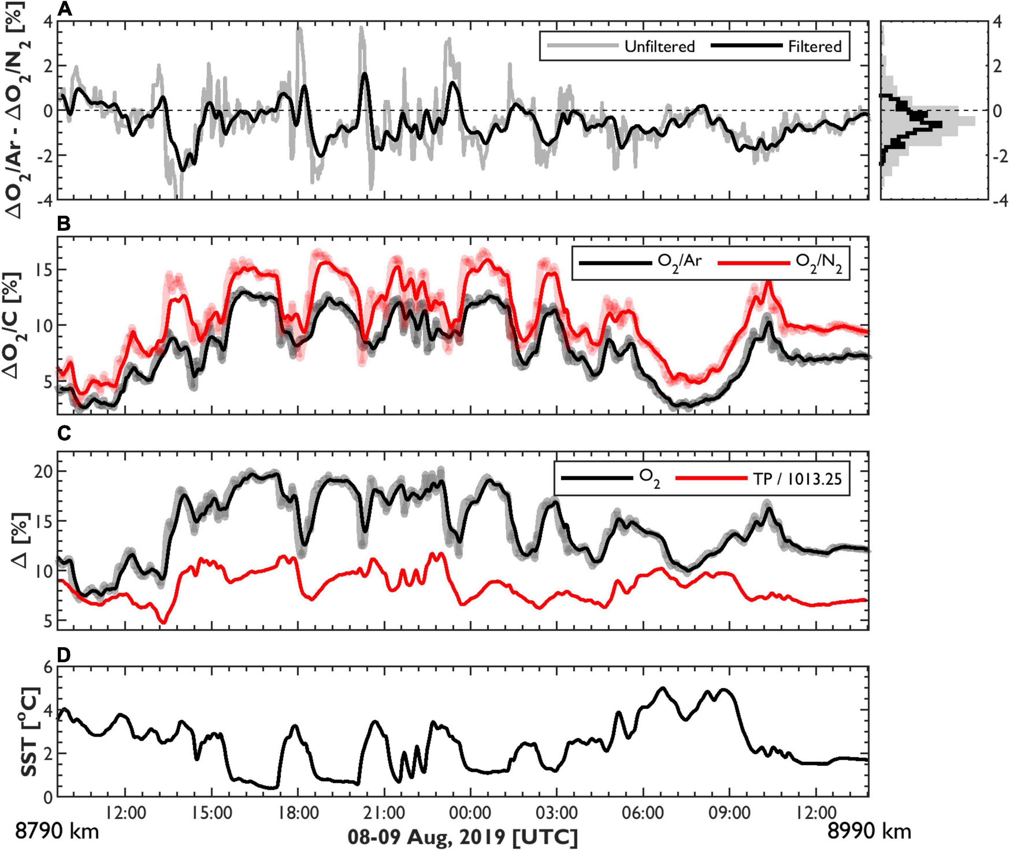
Figure 8. A subset of the 2019 Arctic cruise track showing the occurrence of transient ΔO₂/Ar – ΔO₂/N₂ decoupling resulting from differential response times of the optode, GTD and MIMS. (A) Shows the difference between the unfiltered (gray) and filtered (black) ΔO₂/Ar and ΔO₂/N₂ datasets. The histogram shows the corresponding distribution of offsets. In (B,C), the thick, lighter-colored lines represent unfiltered data, while the bold lines are the filtered signals. Note that the ΔO₂/N₂ data in (B) were shifted up by 2% so signals could be distinguished from ΔO₂/Ar. SST is shown for reference in (D).

In future studies of ΔO₂/N₂-NCP, we recommend the data processing procedures outlined above. Additional data treatment may be required to selectively remove signals clearly impacted by the slower response of the GTD relative to the optode. This procedure could, for example, be facilitated by comparing ΔO₂/N₂ and SST signals. The O₂/N₂ measurement system used in this study was designed to optimize GTD response times (Izett and Tortell, 2020), so the issues described here reflect current instrumentation limitations and are unavoidable without further data filtering. Overall, this problem, while not insurmountable, should motivate continued development of GTD technology with more rapid response times.

Explaining Differences Between ΔO₂/Ar and ΔO₂/N₂

Izett and Tortell (2021) recently developed a one-dimensional model to evaluate the contributions of various physical processes to divergence between ΔO ₂/A r and ΔO₂/N₂ (i.e., ΔN₂/Ar disequilibrium) in the Subarctic NE Pacific. These simulations demonstrated the coupling between seasonal SST trends and ΔN₂/Ar variability in temperate waters. Rapid SST changes and short-term elevated wind events or SLP variability were shown to induce more transient responses, while combined bubble and vertical mixing fluxes contributed to seasonal alterations in baseline ΔN₂/Ar, leading to higher winter values. As we discuss below, our field observations are consistent with these results, and with surface inert gas observations reported elsewhere (Hamme and Emerson, 2006; Hamme et al., 2017).

In the offshore NEP-summer waters, surface ΔN₂/Ar values of ∼0.25% (Supplementary Figure 4) predominantly reflect the influence of summertime warming in increasing gas saturation states, with gas re-equilibration under low-to-moderate wind speeds (typically < 10 m s^–1) maintaining ΔN₂ greater than ΔAr. In contrast, the ΔN₂/Ar anomalies along the offshore section of the NEP-winter cruise (median ∼0.5%) likely reflect cooling and stronger bubble and, to some extent, mixing fluxes, which, respectively, lower and elevate gas saturation states and ΔN ₂/A r. Despite lacking ΔN₂/Ar_deep observations from the winter cruise (archived observations suggest a value close to 0.5%; Hamme et al., 2019), we estimated relatively strong offshore mixing rates (κ_Z ∼4 × 10^–4 m² s^–1; Supplementary Table 1), implying that mixing contributed to the observed ΔN₂/Ar disequilibrium. The influence of vertical mixing was also likely significant in the QCS region, where we observed the largest ΔN₂/Ar disequilibria and negative surface ΔO₂ (Figure 4A). In this region, sedimentary or deep-water denitrification, which has been observed in coastal fjords and inland channels throughout British Columbia (Manning et al., 2010; Bourbonnais et al., 2013) may have elevated ΔN₂/Ar_deep, resulting in the vertical supply of microbially N₂-enriched water into surface waters. This hypothesis is supported by observations of lower N^∗, an indicator of nitrate loss via denitrification (Gruber and Sarmiento, 1997), in the QCS region (range ∼−2 to −6 μmol L^–1 in the upper 500 m), relative to offshore waters of the NEP (Supplementary Figure 5C). As the success of the N₂′ calculations suggest (following section), the influence of vertical mixing on surface ΔN₂/Ar across all sampling regions in NEP-winter was important, and our combined estimates of κ_Z and ΔN₂/Ar_deep capture this process.

In the Arctic, the elevated ΔAr and ΔN₂ we observed (up to 10%; Supplementary Figure 2) exceed most previously reported gas observations in the region (Eveleth et al., 2014; Hamme et al., 2017). However, such conditions can be produced in mixed layer model simulations replicating the conditions encountered before our sampling in northern Baffin Bay (BB) (warming up to 9°C over ∼30 days and mean wind speeds ∼4 m s^–1; simulation results based on the model in Izett and Tortell, 2021; not shown). The resulting positive ΔN₂/Ar disequilibria we observed (median ∼0.5% in BB; Supplementary Figure 4) is consistent with values of ∼0.3–0.7% predicted in these numerical simulations, reflecting the dominant influence of seasonal warming. Although warming increases both ΔAr and ΔN₂, Ar re-equilibrates more rapidly than N₂, causing ΔN₂ > ΔAr. The mixing contribution was less important (mean BB κ_Z ∼1 × 10^–4 m² s^–1). Elsewhere in the Arctic, the high spatial heterogeneity of ΔO₂, ΔAr, and ΔN₂ likely reflects variability in ice cover and environmental forcing via air-sea exchange, SST changes and mixing. Although denitrification may be significant in some Arctic waters, including the shallow shelves of the western Arctic (Reeve et al., 2019), the low ΔN₂/Ar_deep observed throughout our cruise region (Supplementary Figure 5C) suggests that the vertical supply of microbially N₂-enriched water into surface waters was not important in driving ΔO₂/Ar – ΔO₂/N₂ differences.

Evaluating ΔO₂/N₂′ as an NCP Tracer in Field Studies

Across our three cruise dataset, biological O₂ saturation anomalies based on O₂/N₂ measurements were able to replicate the high-resolution heterogeneity in surface productivity captured by the MIMS-based ΔO₂/Ar surveys (Figures 3–5). However, offsets between ΔO₂/Ar and uncorrected ΔO₂/N₂ manifested as important deviations in NCP estimates derived from the respective tracers (Figure 7). Most importantly, in a portion of the dataset (∼15% of the pooled data), ΔO₂/N₂-NCP predicted net heterotrophic conditions (negative NCP), whereas ΔO₂/Ar-NCP was positive (Table 1). Notwithstanding sources of analytical errors (see above), these offsets are largely attributable to physical processes which cause ΔN₂ and ΔAr to diverge. If uncorrected, these effects can have significant consequences for the interpretation of oceanic productivity and trophic status, particularly if NCP estimates are integrated over an annual cycle. Fortunately, such biases can be corrected to a large extent, using the new tracer ΔO₂/N₂′. When we apply these corrections, derived ΔO₂/N₂′ approached ΔO₂/Ar across all cruise regions and sub-regions, and the linear relationship between these tracers was not significantly different than one (Figure 6).

On regional scales, ΔO₂/N₂′-NCP was roughly equivalent to ΔO₂/Ar-NCP, and was typically more accurate than ΔO₂/N₂-NCP (Figure 7). Indeed, in all sampling sub-regions, the median difference between ΔO₂/Ar- and ΔO₂/N₂′-NCP was lower than corresponding differences with ΔO₂/N₂-NCP (Table 1). While the N₂′ calculations were unable to fully eliminate NCP biases, our results nonetheless demonstrate the ability of ΔO₂/N₂′ to reduce NCP estimation errors. For example, offsets between ΔO ₂/Ar- and ΔO₂/N₂′-NCP (red lines in Figure 7B) were typically smaller than NCP errors associated with vertical O₂ mixing fluxes (Table 1) or the ∼20–40% uncertainty in the O₂ gas transfer velocity, k_O2 (gray shading in Figure 7B; Bender et al., 2011; Wanninkhof, 2014). Biases in the ΔO₂/N₂-NCP dataset (black lines in Figure 7B) were often equal to or greater than these other errors. Median mixing biases, estimated from N₂O-based measurements in the NEP (following Izett et al., 2018), or by combining NEMO model- and CTD-derived κ_Z and O₂ observations in the Arctic, ranged from ∼2 to > 20 mmol O₂ m^–2 d^–1, with higher values in nearshore regions. Errors associated with a 20% uncertainty in k_O2 were up to ∼12 mmol O₂ m^–2 d^–1 (mean ∼3 mmol O₂ m^–2 d^–1). Excluding observations where the ΔO₂/Ar – ΔO₂/N₂ offset was > 1.5% (i.e., likely resulting from analytical uncertainties and sampling artifacts), biases between uncorrected ΔO₂/N₂- and ΔO₂/Ar-NCP exceeded the magnitude of the corresponding air-sea and O₂ mixing flux errors in ∼40 and 5% of the dataset, respectively. These values were reduced to ∼10 and 1% after applying N₂′ calculations. This result suggests that uncertainty in ΔO₂/N₂′ will be typically smaller than other main sources of error in NCP calculations. Moreover, ΔO₂/N₂′-NCP more frequently predicted the same metabolic status as ΔO₂/Ar-based estimates in all sub-regions (∼96% of all observations; Table 1). Taken together, these results demonstrate the strong potential of the N₂′ approach for reducing biases in NCP estimates derived from O₂/N₂ surveys, even if offsets between ΔO₂/Ar and ΔO₂/N₂′ cannot be fully reconciled.

Notably, the relative success the N₂′ calculations varied by sub-region. In the NEP (summer and winter), ΔO₂/N₂′ represented a significant improvement over uncorrected ΔO₂/N₂. In parts of the Arctic, however, the benefit of N₂′ is somewhat less clear, as median and pair-wise offsets between NCP calculations were similar in both the ΔO₂/N₂ and ΔO₂/N₂′ datasets. Yet, our analyses suggest that ΔO₂/N₂′ is a less ambiguous NCP tracer, particularly in Baffin Bay where estimates based on ΔO₂/N₂ had the opposite sign to ΔO ₂/A r-NCP in ∼5% of the dataset (compared with 0% in the ΔO₂/N₂′ dataset). In the coastal waters of the Arctic shelf and CAA, where the vertical O₂ mixing bias may overwhelm the ML mass balance, N₂′ calculations are subject to more uncertainty, and may therefore not be necessary. Indeed, in the shelf and CAA regions, median NCP biases based on ΔO ₂/N₂′ and ΔO₂/N₂ (∼0.8 ± 2.1 and 1.1 ± 1.9 mmol O₂ m^–2 d^–1, respectively; uncertainty represents one standard deviation around the mean value) were smaller than the mean mixing biases of ∼6.2 ± 12.1 mmol O₂ m^–2 d^–1. In the nearshore waters of the NEP (QCS region), the O₂ mixing bias (up to ∼90 mmol O₂ m^–2 d^–1) constituted a major component of the ML O₂ mass balance and was higher than NCP biases between the various tracers (∼9 mmol O₂ m^–2 d^–1). However, N₂′ calculations still significantly reduced the large errors between ΔO₂/Ar- and ΔO₂/N₂-NCP. Thus, while N₂′ can reduce NCP errors in both coastal and offshore waters, future work will still need to address challenges relating to the vertical mixing of O₂ in such dynamic regions. In contrast, calculation of ΔO₂/N₂′ will likely be necessary to accurately reflect the true metabolic state of low productivity offshore waters and evaluate seasonal changes in ocean productivity.

Remaining Biases Between ΔO₂/Ar and ΔO₂/N₂′

Notwithstanding sources of measurement and analytical error (further details in Supplementary Material Section 4), remaining biases between ΔO₂/Ar and ΔO₂/N₂′ arise from errors in ΔO ₂/N₂′ computations, which have been estimated by Izett and Tortell (2021) to be ∼0.3%. That work demonstrated the ability of the N₂′ budget to capture the dominant processes driving N₂ evolution in oceanic waters of the offshore NEP. In the present dataset, however, errors are most significant in nearshore regions where the negligence of lateral fluxes likely oversimplifies ΔN₂/Ar dynamics. For example, lateral advection or mixing, freshwater input and ice processes may contribute to divergence between the NCP tracers, while significant water mass transport would produce uncertainty in the environmental histories that we ascribe to our underway observations. These processes are difficult to constrain with simple modeling approaches, and the effects of sea and glacier ice melt on surface seawater ΔN₂/Ar are uncertain (Zhou et al., 2014). Moreover, as we lack broad coverage of direct κ_Z and ΔN₂/Ar_deep observations, misrepresentation of these terms may have contributed to errors in our ΔO₂/N₂′ calculations. However, sensitivity analyses in which we set κ_Z to 0 m² s^–1 or varied κ_Z and ΔN₂/Ar_deep (by 5×10^–5 m² s^–1 and 0.25%, respectively), produced ΔO₂/N₂′-NCP estimates that were typically better than, or equivalent to, ΔO₂/N₂-based values (blue shading in Figure 7B), suggesting that even sparse κ_Z or ΔN₂/Ar_deep measurements can improve the performance of ΔO₂/N₂′ as an NCP tracer. In the absence of direct observations, κ_Z may be derived from numerical simulations or geochemical (e.g., Izett et al., 2018) and hydrographic proxies (Cronin et al., 2015; Haskell et al., 2016), while ΔN₂/Ar_deep can be approximated using archived datasets (Hamme et al., 2019).

Future improvements in the accuracy of ΔO₂/N₂′ will require further refinement of gas flux parameterizations and environmental datasets, particularly in polar regions where current reanalysis products are less accurate (Supplementary Figure 8), and partial ice-cover complicates air-sea flux parameterizations (Islam et al., 2016). Climatological or ancillary datasets of subsurface hydrographic conditions or MLD (e.g., from Argo floats) may be used to better evaluate the time-variability of ML gas evolution, while air-sea flux parameterizations should be validated for the relevant study region. These considerations would enable application of the present approach in unattended optode/GTD deployments from VOS or USV surveys where subsurface observations are presently not feasible.

Conclusion and Outlook

In this paper, we evaluated a new approach for deriving NCP estimates from underway O₂/N₂ surveys, building on the model framework presented in Izett and Tortell (2021). The current study constitutes the first published NCP results based on underway ship-board O₂/N₂ data, and a first attempt at comparing ΔO₂/Ar-NCP and ΔO₂/N₂-NCP. Our results demonstrate the potential to accurately derive NCP from underway O₂/N₂ observations obtained from optode and GTD measurements in a range of ocean regions, including coastal and offshore waters of polar and subpolar seas. These observations, combined with simple computations of the new tracer, ΔO₂/N₂′, can be used to replicate ΔO₂/Ar-based NCP estimates. In some cases, however, NCP estimates based on uncorrected ΔO₂/N₂ may be sufficiently accurate, and future work should endeavor to address other current limitations in NCP calculations (e.g., vertical O₂ mixing flux biases) or further validate the present approach. In all future applications, ship-board gas sensors should be installed as near to the seawater intake as possible and routinely calibrated to optimize data accuracy. For research vessel deployments, the optode should be calibrated over a range of hydrographic conditions using discrete samples collected from the ship’s seawater supply line and surface Niskin bottle (as performed in this study). This practice will minimize potential sampling artifacts related to dissolved O₂ consumption or production in the supply line (Juranek et al., 2010). For remote applications, we recommend calibrating the optode in the laboratory before and after deployments. For all applications, the GTD should be offset-calibrated (at minimum) by comparing in-air GTD measurements with sea level pressure observations, or by assessing the instrument’s accuracy in an equilibrated water sample. When possible, optode/GTD-derived N_2,sat should be evaluated using discrete samples. Successful application of ΔO₂/N₂′ will also rely on accurate parameterization of the environmental conditions for the study region of interest, and careful data handling to minimize analytical errors in the measurements of O₂/N₂. Future work will be aided by the continued development of reanalysis data products and gas sensor technology.

Widespread application of the approach evaluated here has the potential to significantly expand global coverage of NCP measurements from relatively inexpensive autonomous surface O₂ and N₂ measurements. Indeed, we recommend that future surveys incorporate optode/GTD instrumentation or autonomous measurement systems (e.g., Izett and Tortell, 2020) into existing sampling infrastructure on research vessels, VOS (e.g., container ships, cruise ships, sailboats) and in-situ USVs to provide high spatial and temporal coverage of NCP estimates, and improved integration with other autonomous oceanographic and ecological observations. Given the anticipated impacts of climate change on marine biological productivity, such observations will be crucial for evaluating future variability in biogeochemical and environmental conditions, and predicting associated ecosystem-level responses across a range of oceanic environments.

Data Availability Statement

The datasets generated and analyzed in this study are provided on Zenodo in an O2N2 NCP toolbox (https://doi.org/10.5281/zenodo.4024925), which includes underway and discrete gas data, and corresponding hydrographic and environmental observations. The repository also contains Matlab codes and sample calculations for some of the analyses presented in this manuscript. Underway ΔO₂/Ar, O₂ and N₂ data, and corresponding hydrographic and geographic information, are also compiled at Pangaea (NEP data; https://doi.pangaea.de/10.1594/PANGAEA.933345) and the Polar Data Catalogue (Arctic data; https://doi.org/10.5884/13242). Ancillary CTD and TSG data for the NE Pacific and Arctic were provided by the Water Properties group of the Institute of Ocean Sciences (http://www.waterproperties.ca/linep/cruises.php) and the Amundsen Science group of U. Laval (https://doi.org/10.5884/12713 and https://doi.org/10.5884/12715). The CCMPv2 wind speed data were downloaded from https://www.remss.com. The NCEP/NCAR sea level pressure, NARR wind speed and NOAA OI SST reanalysis data products were obtained from https://psl.noaa.gov/data/gridded/. AMSR-2 sea ice data are available at http://www.osi-saf.org/?q=content/global-sea-ice-concentration-amsr-2.

Author Contributions

RI designed the study, conducted most of the field deployments, and led the data analyses and manuscript writing. PT and RH contributed to the study conceptualization. RH, CCM, and AB conducted field sampling for discrete N₂/Ar data, while RH and AB performed the analyses on the discrete samples and provided the resulting data. CM provided assistance with the planning of field deployments and contributed to the analyses of the GTD data. CCM and PT assisted during field deployments. PT provided funding for the work, and contributed significantly to the manuscript writing. All other authors provided feedback on the manuscript writing and structure.

Funding

This work was supported by the Natural Sciences and Engineering Research Council of Canada (NSERC) through a Discovery Grant (PT), an Alexander Graham Bell Canada Graduate Scholarship (RI), and postdoctoral fellowship (CCM). Funding was also provided by the ArcticNet and MEOPAR Networks of Centres of Excellence Canada, through grants to PT, and Polar Knowledge Canada through a Northern Science Training Program grant to RI.

Conflict of Interest

CM discloses a financial interest as vice president of Pro-Oceanus Systems Inc.

The remaining authors declare that the research was conducted in the absence of any commercial or financial relationships that could be construed as a potential conflict of interest.

Publisher’s Note

All claims expressed in this article are solely those of the authors and do not necessarily represent those of their affiliated organizations, or those of the publisher, the editors and the reviewers. Any product that may be evaluated in this article, or claim that may be made by its manufacturer, is not guaranteed or endorsed by the publisher.

Acknowledgments

We would like to thank Susan Allen, Debby Ianson, Laurie Juranek, and two reviewers for their insightful comments on this work. We also thank William Burt, Ross McCulloch, Zarah Zheng, and Holly Westbrook for their assistance collecting field data, and Mark Belton, Erinn Raftery, and Darcy Perin for their assistance analyzing discrete O₂ and N₂/Ar samples. Finally, we wish to thank Marie Robert, many scientists from the Institute of Ocean Sciences and Amundsen Science group, and the Captain and crews of the CCGS Tully and CCGS Amundsen for their significant support during field sampling.

Supplementary Material

The Supplementary Material for this article can be found online at: https://www.frontiersin.org/articles/10.3389/fmars.2021.718625/full#supplementary-material

Footnotes

1. ^ http://www.waterproperties.ca/linep/
2. ^ https://doi.org/10.5281/zenodo.4024925

References

Amundsen Science Data Collection (2020a). CTD-Rosette Data Collected by the CCGS Amundsen in the Canadian Arctic. Arcticnet Inc., arcticnet Inc., Québec, Canada. Processed data. Version 1. Waterloo: Canadian Cryospheric Information Network (CCIN), doi: 10.5884/12713

CrossRef Full Text | Google Scholar

Amundsen Science Data Collection (2020b). TSG Data Collected by the CCGS Amundsen in the Canadian Arctic. Arcticnet Inc., Arcticnet Inc., Québec, Canada. Processed data. Version 1. Waterloo: Canadian Cryospheric Information Network (CCIN), doi: 10.5884/12715

CrossRef Full Text | Google Scholar

Atlas, R., Hoffman, R. N., Ardizzone, J., Leidner, S. M., Jusem, J. C., Smith, D. K., et al. (2011). A cross-calibrated, multiplatform ocean surface wind velocity product for meteorological and oceanographic applications. Bull. Am. Meteorol. Soc. 92, 157–174. doi: 10.1175/2010BAMS2946.1

CrossRef Full Text | Google Scholar

Bender, M. L., Kinter, S., Cassar, N., and Wanninkhof, R. (2011). Evaluating gas transfer velocity parameterizations using upper ocean radon distributions. J. Geophys. Res. 116, 1–11. doi: 10.1029/2009JC005805

CrossRef Full Text | Google Scholar

Bittig, H. C., Körtzinger, A., Neill, C., van Ooijen, E., Plant, J. N., Hahn, J., et al. (2018). Oxygen optode sensors: principle, characterization, calibration, and application in the ocean. Front. Mar. Sci. 4:429. doi: 10.3389/fmars.2017.00429

CrossRef Full Text | Google Scholar

Bourbonnais, A., Lehmann, M. F., Hamme, R. C., Manning, C. C., and Juniper, S. K. (2013). Nitrate elimination and regeneration as evidenced by dissolved inorganic nitrogen isotopes in Saanich Inlet, a seasonally anoxic fjord. Mar. Chem. 157, 194–207. doi: 10.1016/j.marchem.2013.09.006

CrossRef Full Text | Google Scholar

Bushinsky, S. M., and Emerson, S. (2015). Marine biological production from in situ oxygen measurements on a profiling float in the subarctic Pacific Ocean. Glob. Biogeochem. Cycles 29, 2050–2060. doi: 10.1002/2015GB005251

CrossRef Full Text | Google Scholar

Butterworth, B. J., and Miller, S. D. (2016). Air-sea exchange of carbon dioxide in the Southern Ocean and Antarctic marginal ice zone. Geophys. Res. Lett. 43, 7223–7230. doi: 10.1002/2016GL069581

CrossRef Full Text | Google Scholar

Castro de la Guardia, L., Garcia-Quintana, Y., Claret, M., Hu, X., Galbraith, E. D., and Myers, P. G. (2019). Assessing the role of high-frequency winds and sea ice loss on arctic phytoplankton blooms in an ice-ocean-biogeochemical model. J. Geophys. Res. Biogeosci. 124, 2728–2750. doi: 10.1029/2018JG004869

CrossRef Full Text | Google Scholar

Craig, H., and Hayward, T. (1987). Oxygen supersaturation in the ocean: biological versus physical contributions. Science 235, 199–202. doi: 10.1126/science.235.4785.199

PubMed Abstract | CrossRef Full Text | Google Scholar

Cronin, M. F., Pellan, N. A., Emerson, S. R., and Crawford, W. R. (2015). Estimating diffusivity from the mixed layer heat and salt balances in the North Pacific. J. Geophys. Res. Ocean 120, 7346–7362. doi: 10.1002/2015JC011010

CrossRef Full Text | Google Scholar

D’Asaro, E., and McNeil, C. (2008). Air-sea gas exchange at extreme wind speeds measured by autonomous oceanographic floats. J. Mar. Syst. 74, 722–736. doi: 10.1016/j.jmarsys.2008.02.006

CrossRef Full Text | Google Scholar

D’Asaro, E. A., and McNeil, C. (2013). Calibration and stability of oxygen sensors on autonomous floats. J. Atmos. Ocean. Technol. 30, 1896–1906. doi: 10.1175/JTECH-D-12-00222.1

CrossRef Full Text | Google Scholar

Emerson, S. (2014). Annual net community production and the biological carbon flux in the ocean. Global Biogeochem. Cycles 28, 14–28. doi: 10.1002/2013GB004680

CrossRef Full Text | Google Scholar

Emerson, S., and Bushinsky, S. (2016). The role of bubbles during air-sea gas exchange. J. Geophys. Res. Ocean 121, 4360–4376. doi: 10.1002/2016JC011744

CrossRef Full Text | Google Scholar

Emerson, S., and Stump, C. (2010). Net biological oxygen production in the ocean-II: remote in situ measurements of O₂ and N₂ in subarctic pacific surface waters. Deep Sea Res. 1 Oceanogr. Res. Pap. 57, 1255–1265. doi: 10.1016/j.dsr.2010.06.001

CrossRef Full Text | Google Scholar

Emerson, S., Stump, C., Wilbur, D., and Quay, P. (1999). Accurate measurement of O₂, N₂, and Ar gases in water and the solubility of N2. Mar. Chem. 64, 337–347. doi: 10.1016/S0304-4203(98)00090-5

CrossRef Full Text | Google Scholar

Eveleth, R., Cassar, N., Sherrell, R. M., Ducklow, H., Meredith, M. P., Venables, H. J., et al. (2017). Ice melt influence on summertime net community production along the Western Antarctic Peninsula. Deep Sea Res. 2 Oceanogr. Res. Pap. 139, 89–102. doi: 10.1016/j.dsr2.2016.07.016

CrossRef Full Text | Google Scholar

Eveleth, R., Timmermans, M.-L., and Cassar, N. (2014). Physical and biological controls on oxygen saturation variability in the upper Arctic Ocean. J. Geophys. Res. Ocean 119, 7420–7432. doi: 10.1002/2014JC009816

CrossRef Full Text | Google Scholar

Garcia, H. E., and Gordon, L. I. (1992). Oxygen solubility in seawater: better fitting equations. Limnol. Oceanogr. 37, 1307–1312. doi: 10.2307/2837876

CrossRef Full Text | Google Scholar

Garcia, H. E., and Gordon, L. I. (1993). Erratum: oxygen solubility in seawater: better fitting equations. Limnol. Oceanogr. 38:656.

Google Scholar

Gruber, N., and Sarmiento, J. L. (1997). Global paterns of marine nitrogen fixation and denitrification. Glob. Biogeochem. Cycles 11, 235–266.

Google Scholar

Hamme, R. C., Berry, J. E., Klymak, J. M., and Denman, K. L. (2015). In situ O₂ and N₂ measurements detect deep-water renewal dynamics in seasonally-anoxic Saanich Inlet. Cont. Shelf Res. 106, 107–117. doi: 10.1016/j.csr.2015.06.012

CrossRef Full Text | Google Scholar

Hamme, R. C., and Emerson, S. R. (2004). The solubility of neon, nitrogen and argon in distilled water and seawater. Deep Sea Res. 1 Oceanogr. Res. Pap. 51, 1517–1528. doi: 10.1016/j.dsr.2004.06.009

CrossRef Full Text | Google Scholar

Hamme, R. C., and Emerson, S. R. (2006). Constraining bubble dynamics and mixing with dissolved gases: Implications for productivity measurements by oxygen mass balance. J. Mar. Res. 64, 73–95. doi: 10.1357/002224006776412322

CrossRef Full Text | Google Scholar

Hamme, R. C., Emerson, S. R., Severinghaus, J. P., Long, M. C., and Yashayaev, I. (2017). Using Noble gas measurements to derive air-sea process information and predict physical gas saturations. Geophys. Res. Lett. 44, 9901–9909. doi: 10.1002/2017GL075123

CrossRef Full Text | Google Scholar

Hamme, R. C., Nicholson, D. P., Jenkins, W. J., and Emerson, S. R. (2019). Using Noble Gases to Assess the Ocean’s Carbon Pumps. Ann. Rev. Mar. Sci. 11, 1–29. doi: 10.1146/annurev-marine-121916-063604

PubMed Abstract | CrossRef Full Text | Google Scholar

Haskell, W. Z., Prokopenko, M. G., Stanley, R. H. R., and Knapp, A. N. (2016). Estimates of vertical turbulent mixing used to determine a vertical gradient in net and gross oxygen production in the oligotrophic South Pacific Gyre. Geophys. Res. Lett. 43, 7590–7599. doi: 10.1002/2016GL069523

CrossRef Full Text | Google Scholar

Islam, F., DeGrandpre, M., Beatty, C., Krishfield, R., and Toole, J. (2016). Gas exchange of CO₂ and O₂ in partially ice-covered regions of the Arctic Ocean investigated using in situ sensors. IOP Conf. Ser. Earth Environ. Sci 35:012018. doi: 10.1088/1755-1315/35/1/012018

CrossRef Full Text | Google Scholar

Izett, R. (2021). O2N2 NCP Toolbox (Version 2021.04). doi: 10.5281/zenodo.4024925.

CrossRef Full Text | Google Scholar

Izett, R., Manning, C. C., Hamme, R. C., and Tortell, P. D. (2018). Refined estimates of net community production in the Subarctic Northeast Pacific derived from ΔO2/Ar measurements with N₂O-based corrections for vertical mixing. Glob. Biogeochem. Cycles 32, 326–350. doi: 10.1002/2017GB005792

CrossRef Full Text | Google Scholar

Izett, R., and Tortell, P. (2020). The pressure of in situ gases instrument (PIGI) for autonomous shipboard measurement of dissolved O₂ and N₂ in surface ocean waters. Oceanography 33, 13–15. doi: 10.5670/oceanog.2020.214

CrossRef Full Text | Google Scholar

Izett, R., and Tortell, P. (2021). ΔO₂/N₂’ as a tracer of mixed layer net community production: theoretical considerations and proof-of-concept. Limnol. Oceanogr. Methods 1–13. doi: 10.1002/lom3.10440

CrossRef Full Text | Google Scholar

Juranek, L., Takahashi, T., Mathis, J., and Pickart, R. (2019). Significant biologically mediated CO₂ uptake in the Pacific Arctic during the late open water season. J. Geophys. Res. Ocean 124, 1–23. doi: 10.1029/2018JC014568

CrossRef Full Text | Google Scholar

Juranek, L. W., Hamme, R. C., Kaiser, J., Wanninkhof, R., and Quay, P. D. (2010). Evidence of O2 consumption in underway seawater lines: implications for air-sea O2 and CO2 fluxes. Geophys. Res. Lett. 37, 1–5. doi: 10.1029/2009GL040423

CrossRef Full Text | Google Scholar

Kaiser, J., Reuer, M. K., Barnett, B., and Bender, M. L. (2005). Marine productivity estimates from continuous O₂/Ar ratio measurements by membrane inlet mass spectrometry. Geophys. Res. Lett. 32, 1–5. doi: 10.1029/2005GL023459

CrossRef Full Text | Google Scholar

Kalnay, E., Kanamitsu, M., Kistler, R., Collins, W., Deaven, D., Gandin, L., et al. (1996). The NCEP/NCAR 40-year reanalysis project. Bull. Am. Meteorol. Soc. 77, 437–471. doi: 10.1175/1520-04771996077<0437:TNYRP<2.0.CO;2

CrossRef Full Text | Google Scholar

Kana, T. M., Darkangelo, C., Hunt, M. D., Oldham, J. B., Bennett, G. E., and Cornwell, J. C. (1994). Membrane inlet mass spectrometer for rapid high-precision determination of N₂, O₂, and Ar in environmental water samples. Anal. Chem. 66, 4166–4170. doi: 10.1021/ac00095a009

CrossRef Full Text | Google Scholar

Kavanaugh, M. T., Emerson, S. R., Hales, B., Lockwood, D. M., Quay, P. D., and Letelier, R. M. (2014). Physicochemical and biological controls on primary and net community production across northeast Pacific seascapes. Limnol. Oceanogr. 59, 2013–2027. doi: 10.4319/lo.2014.59.6.2013

CrossRef Full Text | Google Scholar

Liang, J.-H. H., Deutsch, C., McWilliams, J. C., Baschek, B., Sullivan, P. P., and Chiba, D. (2013). Parameterizing bubble-mediated air-sea gas exchange and its effect on ocean ventilation. Glob. Biogeochem. Cycles 27, 894–905. doi: 10.1002/gbc.20080

CrossRef Full Text | Google Scholar

Manning, C. C., Hamme, R. C., and Bourbonnais, A. (2010). Impact of deep-water renewal events on fixed nitrogen loss from seasonally-anoxic Saanich Inlet. Mar. Chem. 122, 1–10. doi: 10.1016/j.marchem.2010.08.002

CrossRef Full Text | Google Scholar

McNeil, C., Katz, D., Wanninkhof, R., and Johnson, B. (2005). Continuous shipboard sampling of gas tension, oxygen and nitrogen. Deep Sea Res. 1 Oceanogr. Res. Pap. 52, 1767–1785. doi: 10.1016/j.dsr.2005.04.003

CrossRef Full Text | Google Scholar

Mesinger, F., DiMego, G., Kalnay, E., Mitchell, K., Shafran, P. C., Ebisuzaki, W., et al. (2006). North American regional reanalysis. Bull. Am. Meteorol. Soc. 87, 343–360. doi: 10.1175/BAMS-87-3-343

CrossRef Full Text | Google Scholar

Moore, J. K., Fu, W., Primeau, F., Britten, G. L., Lindsay, K., Long, M., et al. (2018). Sustained climate warming drives declining marine biological productivity. Science 359, 1139–1143. doi: 10.1126/science.aao6379

PubMed Abstract | CrossRef Full Text | Google Scholar

Palevsky, H., and Nicholson, D. (2018). The North Atlantic biological pump: insights from the ocean observatories initiative Irminger Sea Array. Oceanography 31, 42–49. doi: 10.5670/oceanog.2018.108

CrossRef Full Text | Google Scholar

Reeve, J. L., Hamme, R. C., and Williams, W. J. (2019). Tracing denitrification in the Canada Basin: N₂ loss to the atmosphere on the Chukchi Shelf and benthic inputs in deep waters. Deep Sea Res. Part I Oceanogr. Res. Pap. 143, 127–138. doi: 10.1016/j.dsr.2018.11.003

CrossRef Full Text | Google Scholar

Reynolds, R. W., Smith, T. M., Liu, C., Chelton, D. B., Casey, K. S., and Schlax, M. G. (2007). Daily high-resolution-blended analyses for sea surface temperature. J. Clim. 20, 5473–5496.

Google Scholar

Spreen, G., Kaleschke, L., and Heygster, G. (2008). Sea ice remote sensing using AMSR-E 89-GHz channels. J. Geophys. Res 113:C02S03. doi: 10.1029/2005JC003384

CrossRef Full Text | Google Scholar

Steiner, N., Vagle, S., Denman, K. L., and McNeil, C. (2007). Oxygen and nitrogen cycling in the northeast Pacific - simulations and observations at Station Papa in 2003/2004. J. Mar. Res. 65, 441–469. doi: 10.1357/002224007781567658

CrossRef Full Text | Google Scholar

Teeter, L., Hamme, R. C., Ianson, D., and Bianucci, L. (2018). Accurate estimation of net community production from O₂/Ar measurements. Glob. Biogeochem. Cycles 32, 1163–1181. doi: 10.1029/2017GB005874

CrossRef Full Text | Google Scholar

Thomson, R. E., and Fine, I. V. (2003). estimating mixed layer depth from oceanic profile data. J. Atmos. Ocean. Technol. 20, 319–329. doi: 10.1175/1520-04262003020<0319:EMLDFO<2.0.CO;2

CrossRef Full Text | Google Scholar

Tortell, P. D. (2005). Dissolved gas measurements in oceanic waters made by membrane inlet mass spectrometry. Limnol. Oceanogr. Methods 3, 24–37. doi: 10.4319/lom.2005.3.24

CrossRef Full Text | Google Scholar

Uchida, H., Kawano, T., Kaneko, I., and Fukasawa, M. (2008). In situ calibration of optode-based oxygen sensors. J. Atmos. Ocean. Technol. 25, 2271–2281. doi: 10.1175/2008JTECHO549.1

CrossRef Full Text | Google Scholar

Vagle, S., McNeil, C., and Steiner, N. (2010). Upper ocean bubble measurements from the NE Pacific and estimates of their role in air-sea gas transfer of the weakly soluble gases nitrogen and oxygen. J. Geophys. Res. Ocean 115, 1–16. doi: 10.1029/2009JC005990

CrossRef Full Text | Google Scholar

Volk, T., and Hoffert, M. I (1985). “Ocean carbon pumps: analysis of relative strengths and efficiencies in ocean-driven atmospheric CO₂ changes,” in The Carbon Cycle and Atmospheric CO₂: Natural Variations Archean to Present, eds E. T. Sundquist and W. S. Broecker (Washington, DC: American Geophysical Union), 99–110.

Google Scholar

Wanninkhof, R. (2014). Relationship between wind speed and gas exchange over the ocean revisited. Limnol. Oceanogr. Methods 12, 351–362. doi: 10.1029/92JC00188

CrossRef Full Text | Google Scholar

Ware, D. M., and Thomson, R. E. (2005). Bottom-up ecosystem trophic dynamics determine fish production in the Northeast Pacific. Science 308, 1280–1284. doi: 10.1126/science.1109049

PubMed Abstract | CrossRef Full Text | Google Scholar

Zhou, J., Delille, B., Brabant, F., and Tison, J. L. (2014). Insights into oxygen transport and net community production in sea ice from oxygen, nitrogen and argon concentrations. Biogeosciences 11, 5007–5020. doi: 10.5194/bg-11-5007-2014

CrossRef Full Text | Google Scholar