Biomass Mapping for an Improved Understanding of the Contribution of Cold-Water Coral Carbonate Mounds to C and N Cycling

Introduction

Cold-water coral (CWC) carbonate mounds are important marine ecosystems (Roberts et al., 2009). They are topographic seafloor structures that can be several hundreds of meters in height and have accumulated through successive periods of reef development, sedimentation and (bio)erosion over glacial-interglacial periods (Kenyon et al., 2003; Van Weering et al., 2003; Mienis et al., 2007; Roberts et al., 2009). They are hotspots of biomass and biodiversity and provide essential ecosystem functions through nutrient [Carbon (C) and Nitrogen (N)] cycling in a resource-limited deep sea (Henry and Roberts, 2007; van Oevelen et al., 2009; Armstrong et al., 2012). However, significant gaps remain in our understanding of the spatial distribution of their overall biomass and capacity to remineralise organic matter (OM) (De Clippele et al., 2021).

Cold-water coral reefs depend on OM produced at the ocean’s surface to support their growth (Duineveld et al., 2004, 2007; Kiriakoulakis et al., 2005). This OM can be transported to the reef from surface waters through deposition, tidal downwelling, nepheloid layers and deep-water advection (Mienis et al., 2007; Davies et al., 2009; Findlay et al., 2013; Mohn et al., 2014; Soetaert et al., 2016). In addition, when reefs (tens of meters high) accumulate over time to form large CWC carbonate mounds (hundreds of meters high), they can induce a “topographically-enhanced carbon pump” (Soetaert et al., 2016). The mounds large size interrupts the currents, which creates downwelling events bringing OM from surface waters to the mound’s summits and upper flanks (Guinan et al., 2009; Mohn et al., 2014; Rengstorf et al., 2014; Soetaert et al., 2016). Baffling of currents caused by the coral framework can also locally increase the POM concentration at the reefs (Soetaert et al., 2016).

The availability of this food is a major determinant controlling CWCs occurrence and the zonation of macrohabitats on the mounds (De Clippele et al., 2019; Maier et al., 2021). The mound bases are covered by sediments (bio- and siliciclastic sands), pebbles, cobbles and boulders (de Haas et al., 2009). Dense Lophelia pertusa patches characterize the summits of the carbonate mounds, while the flanks of the mounds are covered with patches of coral rubble, dead coral branches and living corals (Kenyon et al., 2003; Van Weering et al., 2003; de Haas et al., 2009; De Clippele et al., 2019; Maier et al., 2021). Dead coral framework is particularly biodiverse as it provides complex micro- and macrohabitats for diverse communities (Jonsson et al., 2004; Henry and Roberts, 2007). It is this living fauna (including e.g., anthozoans, hydroids, ophiuroids, and sponges) that contributes the most to a reef’s capacity to mineralize OM (de Froe et al., 2019; Maier et al., 2019,2020; De Clippele et al., 2021).

Knowing how much live and dead coral framework biomass is present on a CWC reef and their contribution toward OM mineralization is critical information to understand how well the reef is functioning. It also provides a baseline that can help us understand the extent of the potential effects of ocean acidification, warming and decreases in ocean O₂ levels on these vulnerable ecosystems (Hennige et al., 2014, 2015, 2020; Roberts and Cairns, 2014; Sweetman et al., 2017). To estimate biomass and OM mineralization on CWC carbonate mounds, we apply the novel approach by De Clippele et al. (2021). This approach uses surface area measurements of the coral L. pertusa, extracted from high-definition (HD) video frames and combines this with biomass and respiration data. We hypothesize that this method allows to map live and dead coral framework at the CWC Logachev Mound province (LMP) and quantify the ecosystem function of this area.

Methodology

Location

The LMP consists of a cluster of CWC carbonate mounds located on the south-eastern slope of Rockall Bank in the North-East Atlantic (Kenyon et al., 2003; Figure 1). The CWC carbonate mounds are between 5 and 360 m tall, up to a few kilometers long and located between 500 and 1,000 m depth (Kenyon et al., 2003; de Haas et al., 2009). The dominant current direction in the LMP is in a southwest direction, following from a clockwise circumventing flow around Rockall bank (Mienis et al., 2007), while the local diurnal barotropic tide causes cross slope transport in a northwest-southeast direction (Mienis et al., 2007; White, 2007).

FIGURE 1

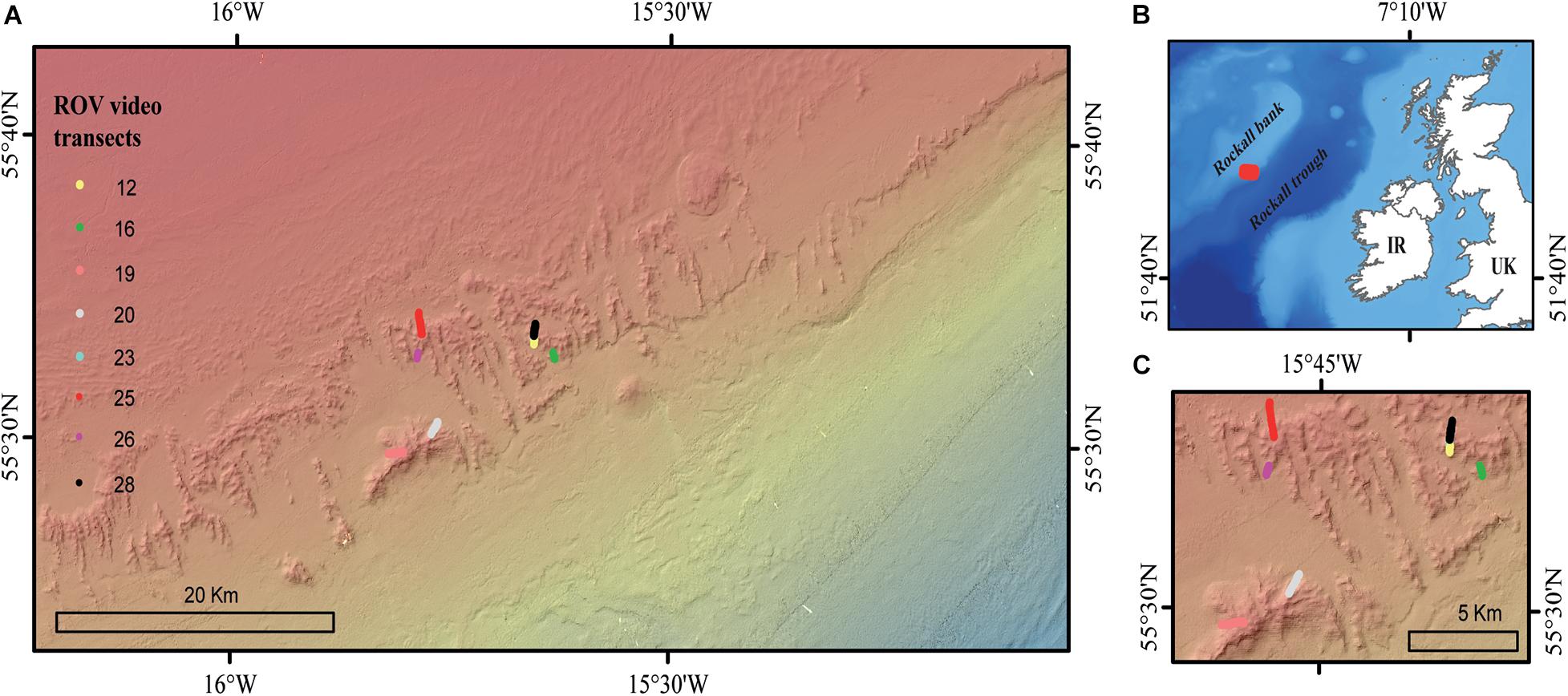
Figure 1. (A) The location of the high-definition ROV video transects in the Logachev Mound Province, (B) the red square indicating the location of the Logachev Mound Province on the southeast shelf of Rockall bank, and (C) a zoomed-in map showing the location of the ROV video transects.

Data

Biological Data

Eight HD video transects were recorded during the Changing Oceans 2012 expedition, RRS James Cook cruise 073 (Roberts, 2013), using the Remotely Operated Vehicle (ROV) Holland-1 (more details in De Clippele et al., 2019; Table 1). Using the software Photoshop CC 2018, video frames were extracted every 500th frame. The video frames were used to measure the surface area of live and dead coral framework (see Section “Biomass Estimation”). The remaining area (total area minus [dead + live] coral framework) was referred to as sediment. However, hard substrates such as pebbles, cobbles, boulders and lithified substrate can also be present (De Clippele et al., 2019; Maier et al., 2021). The ROV was equipped with two parallel pointers, marking a fixed distance of 10 cm on the video frames, which was used to scale the images.

TABLE 1

Table 1. Dive number, location [longitude (Lon.) and latitude (Lat.)], depth range (m), and length (m) of ROV video transects.

In addition, data on the dry weight, C_inorg and C_org stock of the live and dead coral framework, collected with a NIOZ boxcorer (diameter: 50 cm; height 50 cm; surface area ∼0.2 m²) was used. Six cores were collected during the 2017 R/V Pelagia research cruise and used to derive ex situ benthic O₂ and N flux measurements of the CWC community (see Table 1 in de Froe et al., 2019). Photographs were taken of the core surface after sampling and used to calculate the surface area (m²): dry weight (kg) ratio. The photographs were scaled using the dimensions of the boxcorer.

Environmental Data

Particulate organic matter (POM) concentrations were obtained from a POM model with a resolution of 250 m × 250 m (Soetaert et al., 2016). This model provides values that represent the concentration of reactive freshly-produced organic matter available in the water column. These are below the actual measured values of POM concentration, which additionally include refractory organic matter (Soetaert et al., 2016). In addition, terrain variables were extracted from bathymetry data provided by the Irish National Seabed Survey program (INSS) at a 20 m × 20 m resolution. The following topographic terrain variables were derived from the bathymetry data using the ArcGIS 10.1, ESRI Software and the Benthic Terrain Modeller (Wright et al., 2005): depth, slope, aspect (eastness and northness), rugosity (calculated at two spatial scales, using a square kernel window of, respectively, 3 pixels × 3 pixels and 9 pixels × 9 pixels) and bathymetric positioning index (BPI; calculated at two spatial scales using an annulus kernel window with inner and outer radius of, respectively, 3 × 6 and 6 × 9 cells). More information on these variables is provided in De Clippele et al., 2019.

Oxygen and Nitrogen Data

O₂ consumption rates were obtained from ex situ boxcore incubations by de Froe et al. (2019). For live coral framework, an O₂ consumption rate of 6.39 ± 0.32 mmol O₂ kg^–1 dry weight d^–1 (L. pertusa, Madrepora oculata, and Desmophyllum dianthus) was found and for dead coral framework a 0.18 ± 0.01 mmol O₂ kg^–1 dry weight d^–1 was found. For sediment, an average O₂ consumption of 2.4 ± 0.59 mmol m^–2 d^–1 was used, based on the depth-based (500–800 m) turnover rates of O₂ by Glud (2008). Live coral framework released dissolved inorganic N (DIN) mostly as ammonium (NH⁺₄) (Khripounoff et al., 2014), while dead coral framework mostly releases nitrate (NO^–₃) (Maier et al., 2021). For live corals we used an NH⁺₄ release rate of 0.084 ± 0.017 NH₄⁺ mmol kg^–1 d^–1 dry weight (Khripounoff et al., 2014) and for dead coral framework we used an NO^–₃ release rate of 0.053 ± 0.037 NO₃^– mmol kg^–1 d^–1 (Maier et al., 2021). Sediments baffled by coral framework in the LMP release 0.01 ± 0.06 NH₄⁺ mmol m² d^–1 and 0.64 ± 0.37 NO₃^– mmol m² d^–1 while sediments on top of Rockall bank release 0.01 ± 0.06 NH₄⁺ mmol m² d^–1 and 0.52 ± 0.16 NO₃^– mmol m² d^–1 (de Froe et al., 2019). These values are listed in Table 2.

TABLE 2

Table 2. Overview of the O₂ consumption and N values used in this study.

Coral Presence Habitat

Our model area was defined by the habitat suitability model of CWC presence/absence produced by Rengstorf et al. (2014) and covers 253 km². This habitat suitability model was chosen as particulate organic matter (POM) is used as an environmental variable to explain the spatial variability in coral biomass. The POM was calculated by Soetaert et al. (2016) who used the above mentioned habitat suitability model to study benthic respiration and the amount of food supplied to the LMP (Rengstorf et al., 2014). Because the POM model assumed that OM deposition/uptake was increased by a constant factor in the presence of corals, we cannot compare coral-presence habitat with coral-absence habitat (Soetaert et al., 2016).

Biomass Estimation

Biomass is here defined as the live tissue of a specimen. In this study we therefore refer to “(bio)mass” to indicate the differentiation between measuring mass and biomass for, respectively, live and dead coral framework. The approach by De Clippele et al. (2021), was adapted due to a difference in coral morphologies, i.e., the presence of coral thickets at the LMP rather than the globular colonies at the Mingulay Reef (Figure 2). Here, to convert surface area to (bio)mass, (bio)mass data from boxcores collected at the LMP were used (de Froe et al., 2019). The steps are described in detail below and in Figure 3.

FIGURE 2

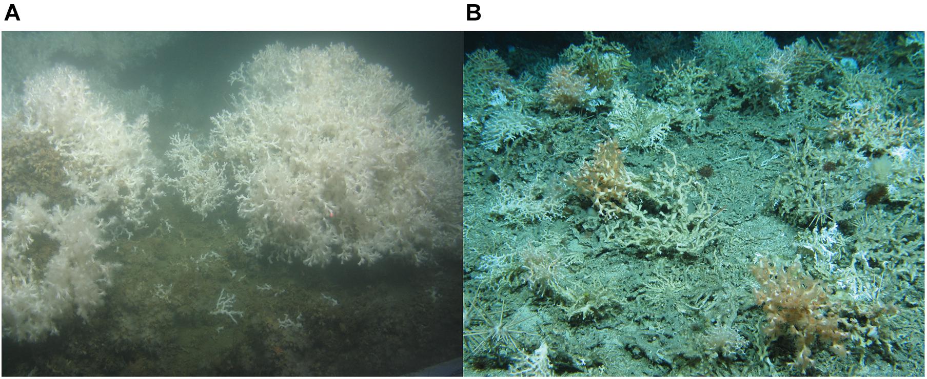
Figure 2. (A) Globular, cauliflower-shaped L. pertusa colonies at the Mingulay Reef Complex sitting on a bed of dead framework and coral rubble, which is partially covered in white zoanthids. (B) Live pink, orange and white coral thickets of L. pertusa and Madrepora oculata at the Logachev Mound Province. The brown/beige colored framework is dead. Image credit: JC073 Changing Oceans Expedition 2012.

FIGURE 3

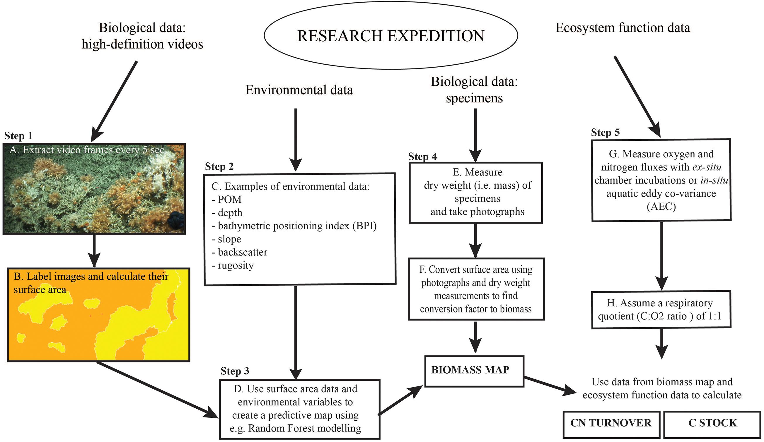
Figure 3. Graphic overview of the approach used in this study. Adapted from Figure 2 in De Clippele et al. (2021).

Image Analyses

Step 1

The video still frames from the HD videos (see Section “Biological Data”) (Figure 3A), were imported in Adobe Photoshop. Bad quality images or images that overlapped were excluded from analyses. In Photoshop, the laser-scale dots, live and dead coral framework were labeled each with a unique color aided by Photoshop’s “quick selection tool” (Figure 3B) (van der Kaaden and De Clippele, 2021). The benthic surface area covered by dead and live coral framework was calculated in R. An R-function (van der Kaaden and De Clippele, 2021) was used to semi-automatically calculate the percentage cover and image size from the labeled images, from which the surface area in m² could be calculated. This faster method is an alternative to the method proposed in De Clippele et al. (2021) where the open-source software ImageJ2 (Greene et al., 1999; Rueden et al., 2017) was used.

Predictive Mapping

Step 2

The surface area data points were imported in ArcGIS and combined in 20 m sub-samples (x-axis). The length of 20 m was chosen as this length gave the most accurate representation of the coral framework variability in relation to the multibeam grid cell size. Then, the ArcGIS Extract Values to Points tool was used to extract the environmental variables (i.e., depth, BPI, slope, rugosity, eastness, northness, and POM) (Figure 3C) associated with each sub-sample data point.

Step 3

The response (i.e., surface area) and explanatory (i.e., environmental) variables were then used to model a predictive map using the Random Forest approach (Figure 3D) with the randomForest package in R (Breiman, 2001). This supervised classification methodology is referred to as a regression tree with a number of simple decision trees. Each tree is based on a bootstrapped sample of the response and explanatory data set. This group of simple trees vote for the most popular class, which is capable of predicting a response when presented with a set of explanatory variables (Cutler et al., 2007; Rogan et al., 2008). Random Forest modeling is commonly used to produce predictive maps (Baccini et al., 2008; Wei et al., 2010; Zhang, 2015; Conti et al., 2019; De Clippele et al., 2021) and provides similar results to approaches using logarithmic regression and Deep Neural Networks (Conti et al., 2019). Here, the training dataset contained one-third of the total data points. This Random Forest model can then be applied to a new set of the same response variables to create a predictive map of the unseen data of the whole area. Correlated environmental variables (<0.5) were removed prior to analyses, using the cor test in R. The importance of the environmental variables in predicting surface area was assessed by calculating the Mean Decrease in Accuracy for each variable to indicate their contribution to the model performance.

To evaluate the uncertainty of the model outputs, we first used a bootstrap technique to produce estimates of model uncertainty (Rowden et al., 2017). This is done by repeating the Random Forest model one hundred times, with the same model but with a replacement random sample of the training data each time. This results in 100 estimates from which the coefficient of variance (CV) was calculated to examine the models output stability. This provides a range of how the Random Forest model output varies and is measured as the standard deviation/mean × 100 (Wei et al., 2010).

Biomass Calculation

Step 4

From the predictive Lophelia reef maps (see step 3), the total amount of live and dead coral framework surface area for the whole habitat suitability area can be extracted and converted to bio(mass) in Excel. To convert live and dead coral framework to (bio)mass, data provided by de Froe et al. (2019) was used (Figure 3E). de Froe et al. (2019) reports the density (kg dry weight m^–2) of live and dead coral framework per boxcore sample (Table 3). From the known surface area of the boxcorer (see Section “Biological Data”), the dry weight of live and dead coral framework per boxcore sample was calculated (kg dry weight boxcore^–1). The benthic surface area of live and dead coral framework from boxcore photographs (Supplementary Materials) was then used to calculate a conversion factor of live/dead coral framework surface area to live/dead coral framework dry mass for each boxcore sample. The mean conversion factor of 8.01 ± 5.52 kg m^–2 and 33.78 ± 6.27 kg m^–2 for live and dead coral framework, respectively, was then used to convert benthic surface area measurements from the HD video extracted frames to skeletal dry weight (kg dry weight) (Figure 3F), i.e., dry weight (kg) = video surface area (m²) × conversion factor (kg m^–2). From this, the biomass (live tissue mass) was calculated using the linear relationship between tissue dry weight and tissue and skeletal weight with the following equation from Hennige et al. (2014): TDW = 0.0415 (TWW + SDW) + 0.0849. With TDW = tissue dry weight (g) = SDW^∗ 5%; TWW = tissue wet weight (g); SDW = skeletal dry weight (g) (De Clippele et al., 2021; Hennige et al., 2014). Sediment were calculated as the remainder (total area minus [dead + live] coral framework). The above conversion calculation was also used in the ArcGIS raster calculator tool to convert the surface area predictive map to a (bio)mass. The standard deviation of the conversion factors was used to calculate the absolute minimum, mean and maximum biomass (see the “Results” section and Supplementary Materials).

TABLE 3

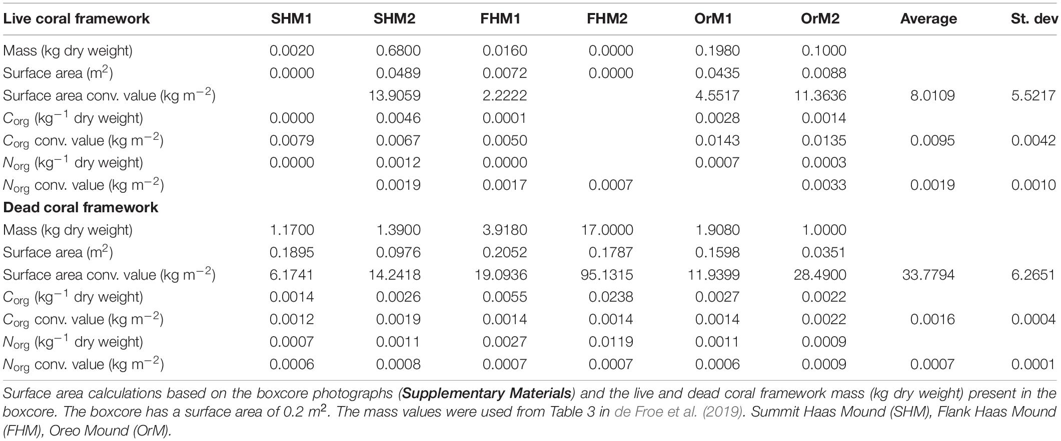
Table 3. Table showing the calculation of the average conversion values and standard deviations used in step 4 and step 5.

Carbon and Nitrogen Turnover and Stock

Step 5

The total biomass and sediment surface area data was used to calculate the yearly C and N turnover for the area, using O₂ consumption data reported in literature (Table 2 and Figure 3G). Carbon and N turnover are here defined as the conversion of ingested food into biomass and loss by respiration as CO₂ and DIN. The C turnover is calculated from the total O₂ consumption assuming a respiratory quotient (C:O₂ ratio) of 1:1 (Glud, 2008) (Figure 3H). This does not account for temporal changes in O₂ consumption that the coral might experience during its lifetime, as this data is currently not available. The live and dead coral framework were multiplied with their respective DIN release rates. More details on this calculation can be found in Step 3 in De Clippele et al. (2021).

In Table 3 by de Froe et al. (2019), the percentage of C_org and N_org of live and dead coral framework per boxcore sample are reported. The C_org and N_org stock of live and dead coral framework per boxcore sample was obtained by multiplying the percentage C_org and N_org content of live and dead coral framework with their total dry weight (C or N kg^–1 dry weight). These values were used to calculate a mean conversion factor for the mass calculated in step 3 to C_org and N_org (Table 3). The C_inorg stock was calculated by multiplying the CaCO₃ mass by 0.12 (Windholz et al., 1983; De Clippele et al., 2021). To account for uncertainties the absolute minimum, mean and maximum CN turnover and C stock were calculated (see the “Results” section and Supplementary Materials).

Results

Predictive Maps

Our model predicts live coral framework covering 8 km² (3%) and dead covering 115 km² (45%) of the CWC habitat area. The remaining 130 km² (51%) is therefore considered to consist of sediment.

The environmental variables used in the mean live coral framework Random Forest model explained 65.54% of the variation in the data. The environmental variables that contributed most to explaining the spatial variability in the amount of live coral framework were BPI (inner cell radius 6 × outer cell radius 9), POM concentration and rugosity (9 × 9 cells) (Figure 4). The live coral framework biomass map (Figure 5) illustrated that the highest live coral biomass is located on the summits of the mounds. The study area contained a total live coral framework skeletal mass of 64,054 T C_inorg (range: 62,280–77,635 T) and biomass of 13,117 T C_org (range: 12,754–15,899 T). Our model results showed highest uncertainty at deeper depths and at the most eastern mounds (Figure 6).

FIGURE 4

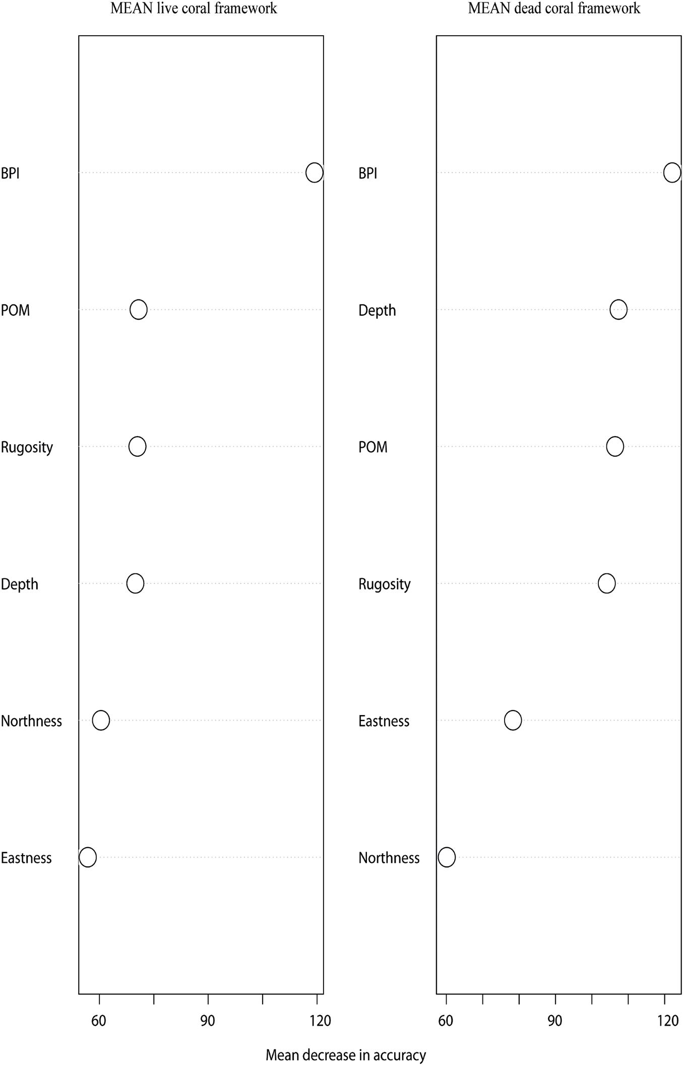
Figure 4. Mean Decrease in Accuracy plots of the mean live and dead coral framework Random Forest model indicating what the contribution of each variable is to the model performance. When the Mean Decrease Accuracy value is higher for a certain variable, the removal of this variable from the model will decrease the model’s performance.

FIGURE 5

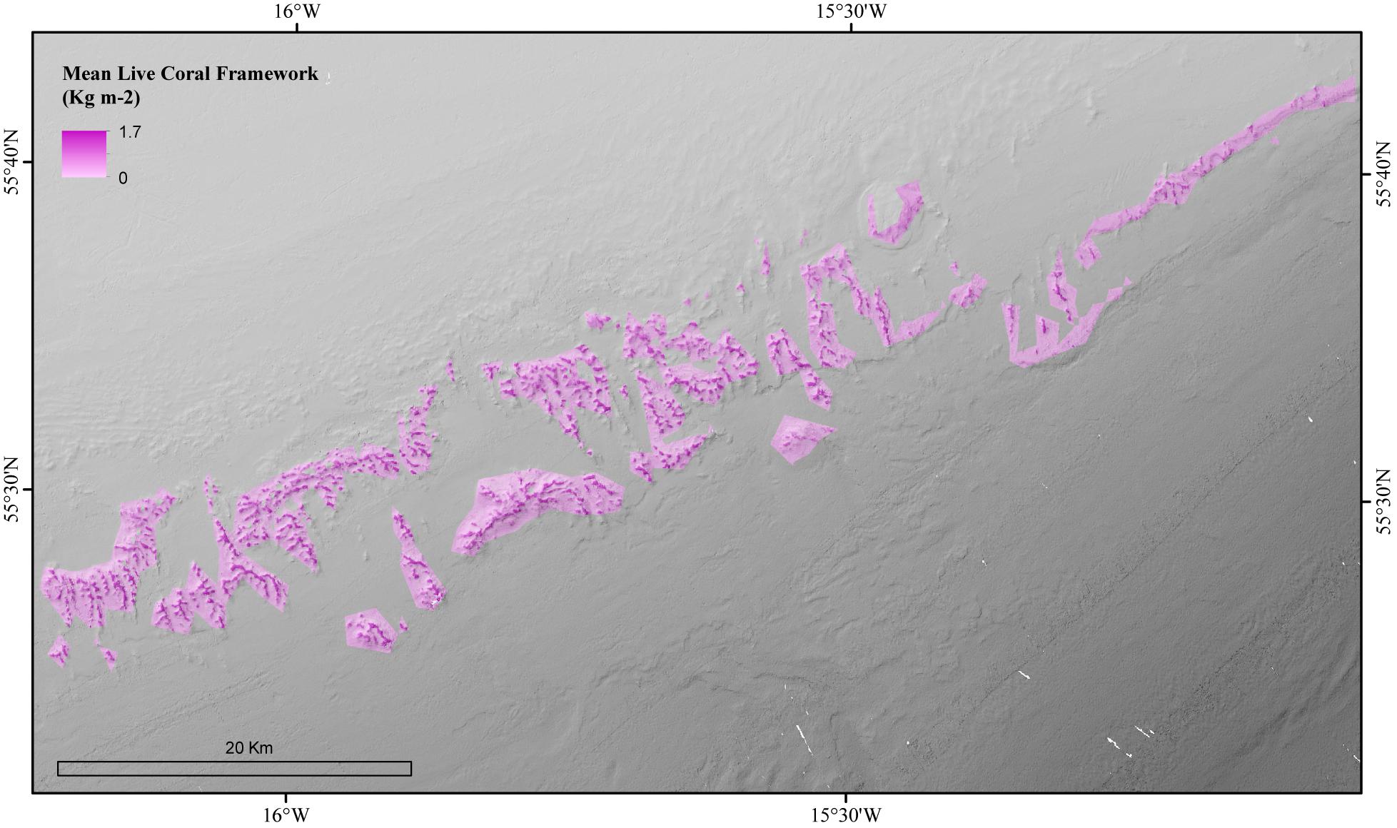
Figure 5. Modeled amount of the mean biomass (Skeletal weight + live tissue weight) of live coral framework in the coral habitat suitability model area of the Logachev Mound Province.

FIGURE 6

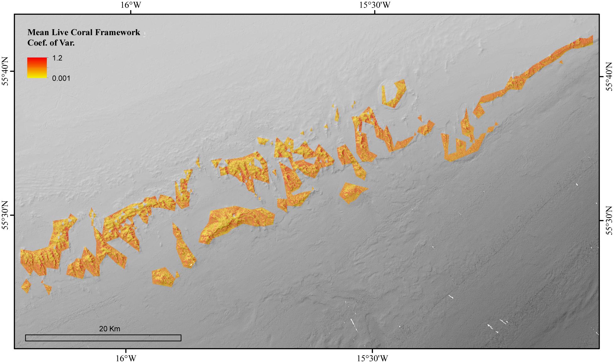
Figure 6. The Coefficient of Variation for the Random Forest model of the mean biomass for live coral framework in the coral reef habitat area of the Logachev Mound Province.

The environmental variables used in the mean dead coral framework Random Forest model explained 54.21% of the variation in the data. The environmental variables that contributed most to explaining the spatial variability in the dead coral framework were BPI, depth and POM (Figure 4). The dead coral framework predictive map (Figure 7) showed that the highest mass is located on the northeast flanks and on the summits of the mounds, and that it decreases with depth. The area has a total mean dead framework skeletal mass of 2,875,706 T C_inorg (range: 3,485,828–4,357,435 T) and variability was also here higher at depth and the most eastern mounds (Figure 8).

FIGURE 7

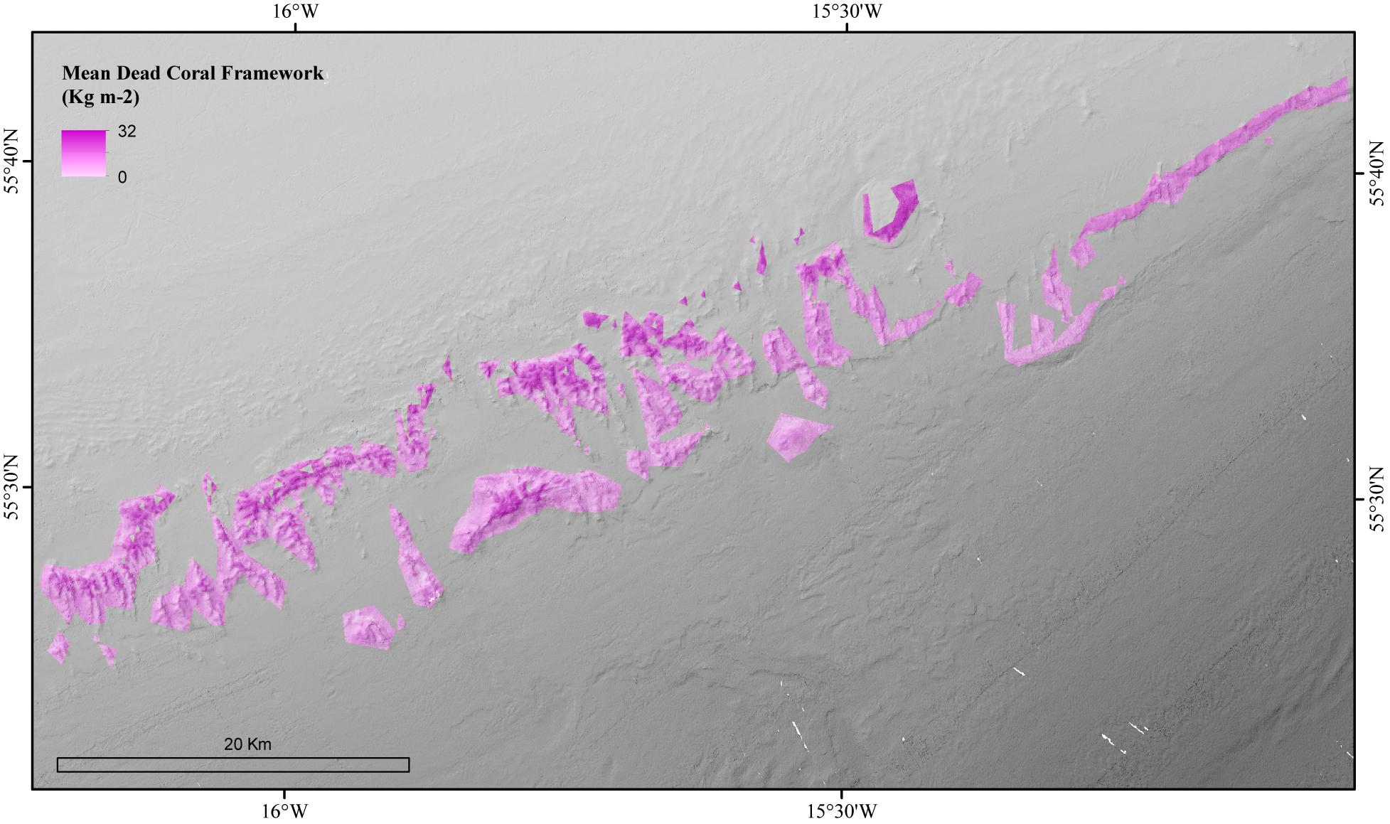
Figure 7. Modeled amount of the mean biomass of dead coral framework in the coral habitat suitability model area of the Logachev Mound Province.

FIGURE 8

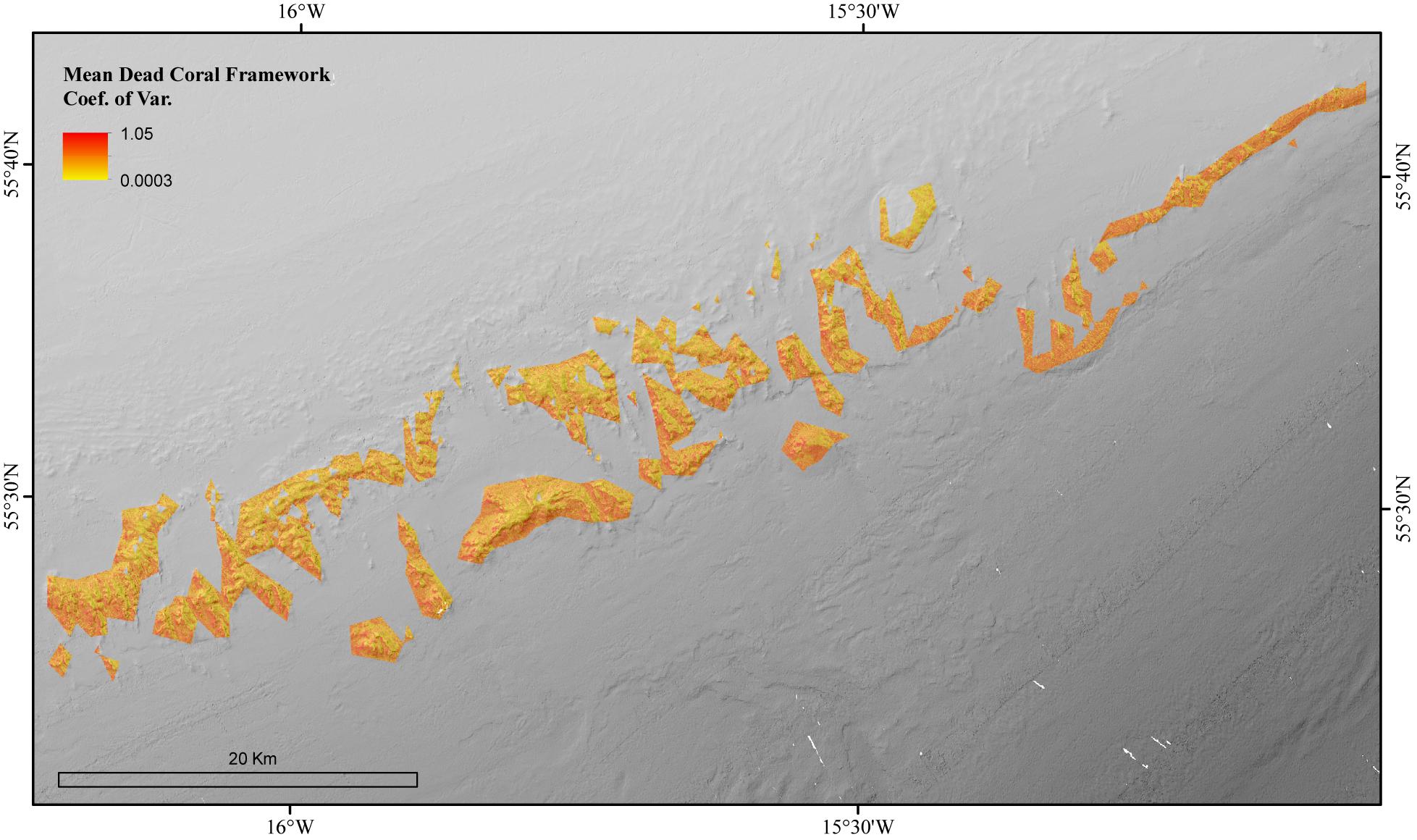
Figure 8. The Coefficient of Variation for the Random Forest model of the mean biomass for dead coral framework in the coral reef habitat area of the Logachev Mound Province.

Stock and Turnover of Carbon and Nitrogen

In the live coral framework a mean of 7,686 T C_inorg (range: 7,474–9,316 T), 607 T C_org (range: 330–1,061 T) and 122 T N_org (range: 119–148 T) is stored. The dead coral framework stores a mean of 465,085 T C_inorg (range: 418,299–522,892), 6 T C_org (range: 0–16 T), and 3 T N_org (range: 2–3 T). On average 0.3 kg m^–2 dry weight of live coral framework and 15.3 kg m^–2 dead coral framework is present in the area according to the predictive maps. Largest C_inorg turnover was found for the dead framework, reaching an annual rate of 3,056 T yr^–1 (49%) (range: 2,596–3,626 T C yr^–1), followed by live coral framework with 1,793 T yr^–1 (29%) (range: 1,656–2,828 T C yr^–1) (Table 4). The fine sediment area turned 1,386 T C_inorg yr^–1 (22%) (range: 1,512–1,216). The total C_inorg turnover at the LMP is 6,235 T C year^–1 (range: 2,596–7,670 T C year^–1), corresponding to an O₂ consumption of 5.64 mmol m^–2 d^–1 (range: 5.21–6.44 mmol O₂ m^–2 d^–1). Dead coral framework turned 290–1,989 T, sediments 432–919 T, and live framework 53–286 T N_inorg year^–1. The total at the LMP was 973–3,194 T N_inorg year^–1.

TABLE 4

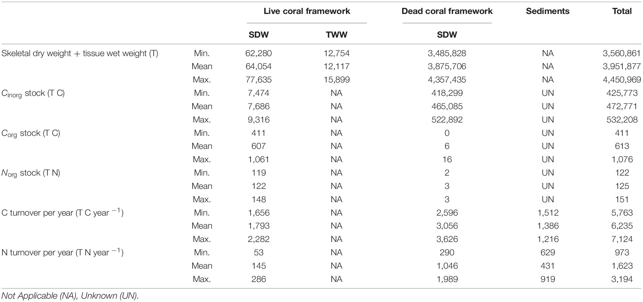
Table 4. Overview of the minimum, mean and maximum (bio)mass, organic and inorganic carbon (C), organic nitrogen (N) stock masses, together with the mass of C and N turned over by live and dead coral framework and sediments.

Discussion

This study applied a new methodology to map live and dead coral framework biomass at the Logachev Mound Province. These biomass maps were used to estimate region-scale inorganic CN turnover, as well as the organic and inorganic CN standing stocks. Even though the reefs at the LMP occur in relatively deep and under food-limited waters compared to shallower inshore reefs (De Clippele et al., 2021) they contribute significantly to the global CN turnover and CN stock. This is as CWC mounds in the LMP, cover a large area and form big mounds due to their ability to persist over glacial-interglacial time scales. This work advances our growing knowledge of their significance to remineralise OM, a criteria used to define Ecologically or Biologically Significant Areas (EBSAs) (Titschack et al., 2015; Johnson et al., 2018).

Distribution of Dead and Live Coral Framework

Spatial differences in environmental conditions drive the small and large scale patterns in biomass observed at the LMP. This study showed that bathymetric positioning index (BPI) is the most important environmental predictor of both live and dead coral framework. This is as coral carbonate mounds form through periods of successive reef development (Roberts et al., 2009). When reef growth dominates over erosion, many small reefs will cover the surface of the mound before they merge and continue the development cycle (Roberts et al., 2009). These smaller reefs coincide with positive BPI values across the LMP (De Clippele et al., 2017). Our predictive biomass map also indicates that live coral framework is predominantly located on the summits of the mounds, which can largely be explained by the higher amount of available POM. In these relative food-limited waters, the supply of POM, i.e., their food, from surface water to the reefs is important to support the high metabolic C demand of the live coral framework (Davies et al., 2009; Roberts et al., 2009). Soetaert et al. (2016) suggest that the high elevation of the coral carbonate mounds induces downwelling and hence POM supply from the ocean surface, a concept described as topographically-enhanced carbon pump. The baffling created by the coral framework can locally increase the POM concentration measured on the reefs (Soetaert et al., 2016). These higher POM concentrations, in turn, can increase the biomass of the live coral framework. This positive feedback loop could explain why the prediction of live coral is strongly driven by POM concentration. The explanatory power of POM could increase even more if a higher resolution POM model would be used. Reduced POM supply linked with bio- and hydrodynamic erosion are the likely causes for the observed reduction in dead coral cover at greater depths (Roberts et al., 2009). This is also shown by Maier et al. (2021), where more degraded coral framework is found at deeper depths and less degraded framework at more shallow depths. Live corals form complex three-dimensional frameworks, and increase the local terrain roughness (Jenness, 2002). Rugosity, a measure of terrain roughness, therefore, represents the third most important variable explaining the prediction of live coral at the LMP.

Our model predicted more dead than live coral framework in the Logachev Mound Province, which is supported by previous studies on CWC reefs (De Clippele et al., 2019, 2021; de Froe et al., 2019; Maier et al., 2021). De Clippele et al. (2019) and Maier et al. (2021) calculated the percentage cover from ROV videos and found that dead coral framework covered 35–93% and live coral framework covered 3–25% of the transects at the LMP. This study found that dead coral framework surface area covered 45%, compared to live coral framework covering 3% of the area. Here, we report 60 times more dead framework mass than live coral mass in the area, which is twice as much as reported by earlier studies (27 times; de Froe et al., 2019). de Froe et al. (2019) based this difference in dry mass on collected boxcores, while here, the whole area is accounted for by means of predictive modeling. Other studies, such as Conti et al. (2019) have calculated the percentage of dead and live coral framework using video mosaic segmentation and classification approaches. They found that the Piddington Mound has 33–43% dead framework (rubble + dead coral framework), 2–3% live coral framework and 48–58% sediments (incl. dropstones) (Conti et al., 2019). While this is similar to what was found in our area, the Piddington mound has a spatial extent of approximately 40 m × 60 m and is one of the smaller mounds found in the Belgica Mound Province. The percentages of the substrates found will vary depending on the extent and the spatial heterogeneity of CWC reef area analyzed. The latter underlines the important contribution of representative sampling techniques and predictive models to more accurately represent CWC framework surface area coverage and biomass. Dead coral framework is important as it facilitates the high biodiversity typical of CWC reefs (Henry and Roberts, 2007) and contributes substantially more to reef fauna biomass and benthic fluxes (de Froe et al., 2019; De Clippele et al., 2021; Maier et al., 2021). Live corals protect themselves against colonization, for example by production of mucus (Freiwald, 2002; Wild et al., 2008; Buhl-Mortensen et al., 2010). In contrast, dead, unprotected coral framework is more easily colonized and provides the majority of micro- and macrohabitats in a CWC reef (Mortensen and Fosså, 2006; Buhl-Mortensen et al., 2010).

Oxygen Consumption and Nitrogen Release

Cold-water coral reefs are hotspots of O₂ consumption and N release, i.e., OM mineralization (van Oevelen et al., 2009; Cathalot et al., 2015; de Froe et al., 2019; De Clippele et al., 2021; Maier et al., 2021). The average C turnover at the LMP, which we derived from O₂ consumption measurements, was 1–3.4 times the global average for a soft-sediment area at the same depth (Glud, 2008). Dead coral framework contributed 49%, live coral framework 29%, and sediments 22% to the total C turnover of the area. At the same time, the reefs at the LMP released 1.9 times more DIN compared to adjacent soft-sediment grounds (de Froe et al., 2019). Here the majority of the DIN was released in the form of NO^–₃ by both dead coral framework (64% of the total N turnover) and sediments (27% of the total N turnover), while NH⁺₄ was released by live coral framework (9% of the total N turnover). It should be noted that the partitioning of DIN release in NH₄⁺ and NO₃^– originates from the model assumption, i.e., that live cold-water corals typically release ammonium as metabolic end product (Khripounoff et al., 2014), while dead framework and sediment release mostly nitrate, due to the activity of nitrifying microorganisms (de Froe et al., 2019; Maier et al., 2021). Tidal induced upwelling of this nutrient-rich reef water could promote new phytoplankton primary production in the surface waters, which in turn would increase OM export to the reef (Davies et al., 2009; Eisele et al., 2011; Hebbeln et al., 2014; Soetaert et al., 2016). Such a loop has been suggested for cold-water coral ecosystems at the shallower Porcupine Bank (White et al., 2005) and could explain how cold-water coral reefs are sustained in the relative resource-poor deep sea. If such a loop is also present at the deeper LMP remains to be determined.

However, it is important to note that the C turnover reported in this study (5.21–6.44 mmol C m^–2 d^–1) is 3–12 times lower than previously reported respiration measurements (van Oevelen et al., 2009; de Froe et al., 2019) (11–75 mmol C m^–2 d^–1). There are three reasons why we might observe this difference. Firstly, in contrast to previous studies, our study accounted for the spatial variability in the biomass of the coral framework across the whole region and revealed that on average 51% is covered by sediments, 45% by dead coral framework, and 3% by live coral framework. Respiration measurements collected by Aquatic Eddy-Correlation (AEC) or boxcore samples are not able to grasp the spatial heterogeneity of such a large area (de Froe et al., 2019; De Clippele et al., 2021). Our study therefore provides a more accurate representation of the total C and N turnover in the area, as it accounts for the spatial complexity.

Secondly, our calculations might be an underestimation as the physical structure of the coral framework baffles sediment (de Haas et al., 2009; de Froe et al., 2019). This type of sediment has a higher OM concentration and C turnover rate (5.32 ± 0.59 mmol O₂ m^–2 d^–1, de Froe et al., 2019) compared to non-reef sediments adjacent to the reefs (de Froe et al., 2019; de Haas et al., 2009). Given that the area that is covered by live and dead coral framework, it will also contain baffled sediment which could significantly increase the total OM mineralization capacity of the area (de Haas et al., 2009). To illustrate the potential contribution of the baffled sediments to the LMP carbon turnover, we assume the area covered by live and dead coral framework is also covered by baffled sediments and add this to our calculation. In this scenario, the result suggests that communities associated with dead coral branches would contribute a mean of 33% (3,056 T C year^–1), baffled sediments 33% (3,025 T C year^–1), sediments 15% (1,389 T C year^–1), and live coral framework 19% (1,793 year^–1) to the total benthic C turnover at the LMP. If we recalculate the C turnover per square meter for this new scenario, a total mean of 8.34 mmol C m^–2 d^–1 is found instead of a mean of 5.64 mmol C m^–2 d^–1. This indicates that cold-water coral carbonate mound sediments might play a much more important role in the C turnover of CWC reefs and carbonate mounds than previously thought.

Thirdly, our predictive maps indicate that in situ measurements by de Froe et al. (2019) were deployed in areas with relatively high coral framework cover (Figure 9). This might provide an overestimation that does not reflect the spatial variability of the C turnover in the area. The Oreo Mound, where we found a particularly high live coral framework cover (Figure 9A), showed the highest AEC O₂ flux of 45.3 mmol m^–2 d^–1 (de Froe et al., 2019). In contrast, the Haas Mound, which contained a lower live coral framework coverage near the AEC deployment site (Figure 9A) showed an O₂ flux of 11.5–22.4 mmol m^–2 d^–1 (de Froe et al., 2019). This indicates that live coral patches are hotspots of metabolic activity within the reef and highlights the importance of understanding the spatial distribution of live and dead coral framework and sediments when planning research equipment deployments.

FIGURE 9

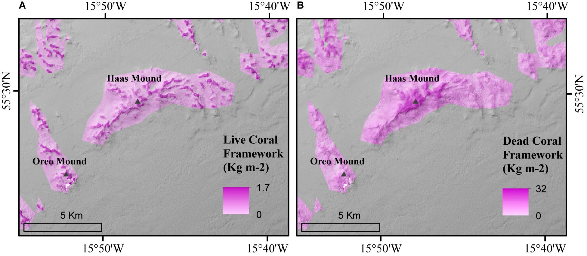
Figure 9. Triangles represent the location of AEC deployment by de Froe et al. (2019) in both the predictive (A) live and (B) dead coral framework map.

Similar to the Mingulay Reef, dead coral framework at the LMP contributes to the majority (49%) of the C turnover (De Clippele et al., 2021). This is expected as cold-water coral carbonate mounds consist of predominantly dead coral framework as discussed above. At the Mingulay Reef, the fauna associated with dead coral framework contributes ∼6 times more to C turnover compared to live coral framework. This is a larger difference compared to the LMP where the fauna associated with dead coral framework contributes only ∼1.7 times more. At Mingulay Reef, a higher biomass of fauna grows on the dead coral framework, hence turning over more C than the live corals (Kazanidis et al., 2016; De Clippele et al., 2021). This biomass difference may be caused by the reefs’ shallower depth and the higher surface primary production above Mingulay Reef (0.048 g C_org m^–3 d^–1), compared to the LMP (0.0067 g C_org m^–3 d^–1) (Tyberghein et al., 2012; Assis et al., 2018; De Clippele et al., 2021) (Table 5). This results in an annual PP over the LMP of 6,194 T C year^–1 and 294 T C year^–1 at the Mingulay Reef (Tyberghein et al., 2012; Assis et al., 2018; De Clippele et al., 2021).

TABLE 5

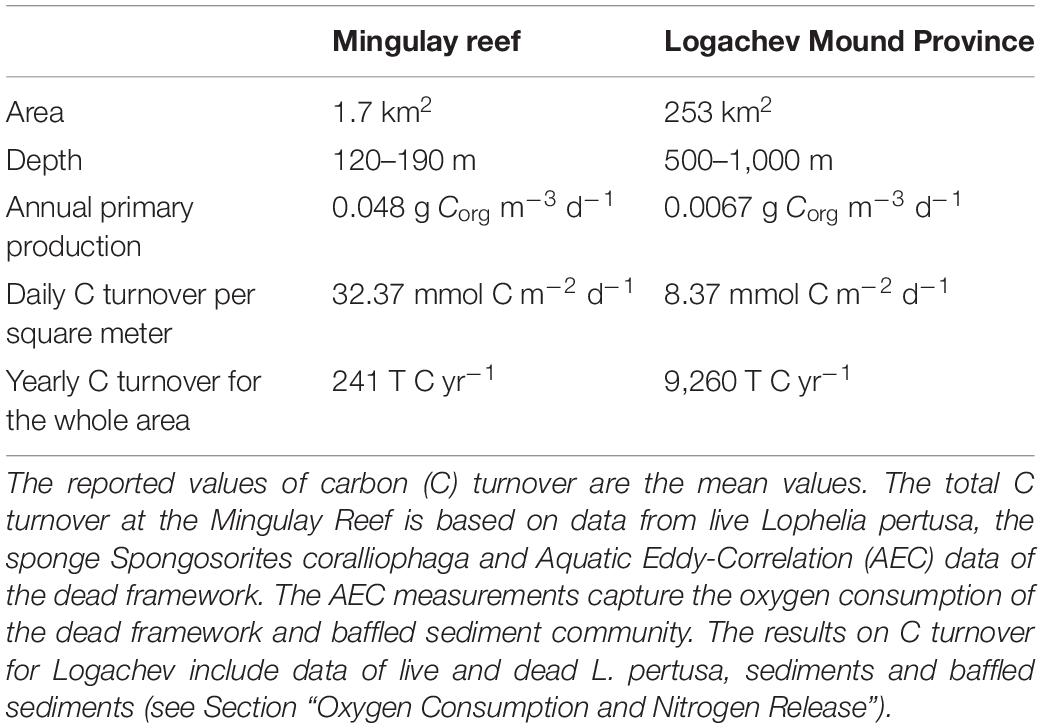
Table 5. Overview of key differences between the Mingulay reef (De Clippele et al., 2021) and the Logachev Mound Province.

How Much Organic Matter Is Required to Sustain the Deep Reefs?

From the annual C and N turnover of the coral presence habitat in the LMP area, we estimate a minimum annual C requirement of 5,763–7,124 T C year^–1 and 973–3,194 T N year^–1. Using the parametrisation by Suess (1980), the amount of particulate organic carbon reaching the seafloor from the sea surface (annual primary production: 6,194 T C year^–1) via deposition was estimated to be 511–322 T C year^–1 for the shallowest (500 m) and deepest point (800 m) of LMP reef habitat area, respectively. This indicates that almost the entire primary production, i.e., 91–95% (5,252–6,802 T C year^–1), would have to be supplied through tidal downwelling, nepheloid layers, lateral deep-water advection and/or by the topographically-enhanced carbon pump (Duineveld et al., 2004; White et al., 2005; Mienis et al., 2007; Soetaert et al., 2016). Our study suggests that the C requirement of the reef could be higher than the yearly PP over the area of 6,194 T C year^–1 (Tyberghein et al., 2012; Assis et al., 2018) depending on seasonal PP and/or biomass variability. This could mean that the PP right above the area might not be sufficient to sustain the reef and highlights the importance of the supply of food trough advection from the wider area, bottom currents together with material retention and recycling of waste material on the reef, in particular during winter food limitation (Maier et al., 2020, 2021). For example, studies have indicated that the reef could benefit from nitrification (re-utilization) of faunal-produced NH⁺₄ (Maier et al., 2020, 2021) and utilization of dissolved OM, which is produced by the corals as mucus (Wild et al., 2004). The dependence of the reef’s function on these alternative supply mechanisms appears greater at the LMP compared to the Mingulay Reef (De Clippele et al., 2021) (Table 5), and is likely due to their location at greater depths with comparatively lower food flux. The supply of food needed to sustain the reef could be severely impacted by climate-induced changes in primary production, local hydrodynamical food supply, which could have severe implications for the survival and functioning of CWC reefs.

Conclusion

Biomass maps can guide sampling and monitoring expeditions and our current approach can be applied to other habitats, to provide large-scale maps of biomass, hotspots of metabolic activity and nutrient mineralization, in particular in the understudied, but large deep-sea realm. The predictive power of this approach can be improved by adding more coral surface area data, especially where the coefficient of variation of the map is higher. Additional local measurements on nutrient cycling, high resolution multibeam data (De Clippele et al., 2019) or more environmental variables (e.g., hydrodynamics) and the use of photo mosaics (Bodenmann and Thornton, 2017; Conti et al., 2019; Price et al., 2019) could further improve our understanding how complex habitats contribute to nutrient cycling. Biomass maps can also advice on the most optimal locations to collect AEC respiration data, to ensure a representative amount of habitat complexity is captured in the measurements (Rovelli et al., 2015; De Clippele et al., 2021). Alternatively, AEC deployments could be used to ground truth the biomass maps. Understanding how much dead and live coral framework is present in this area is especially important in deeper reefs such as the LMP, where ocean acidification threatens to dissolve dead coral framework (Hennige et al., 2015). If the dead coral framework dissolves, not only will the habitat of CWC reef organisms disappear (Kazanidis et al., 2016; Maier et al., 2021), but C and N demineralization, and sediment baffling will diminish. This may ultimately reduce primary production in surface waters, affecting the CO₂ being extracted from the atmosphere. Consequently, these effects will negatively impact the existence of the CWC mounds in the LMP and the overall functioning of the area.

Data Availability Statement

The raw data supporting the conclusions of this article will be made available by the authors, without undue reservation, to any qualified researcher.

Author Contributions

LDC: conceptualization, writing, and methodology. AVDK, SRM, and EDF: review and editing of the manuscript and methodology. JMR: review and editing of the manuscript. All authors contributed to the article and approved the submitted version.

Funding

LDC, EDF and JMR acknowledge funding from the EU Horizon 2020 ATLAS (Grant Agreement No. 678760 to JMR) and iAtlantic projects (Grant Agreement No. 818123 to JMR). SRM was funded by the Royal Netherlands Institute for Sea Research (Grant 864.13.007). AVDK was supported by collaboration funding between Utrecht University and the Royal Netherlands Institute for Sea Research.

Author Disclaimer

This manuscript reflects the authors’ view alone, and the European Union cannot be held responsible for any use that may be made of the information contained herein.

Conflict of Interest

The authors declare that the research was conducted in the absence of any commercial or financial relationships that could be construed as a potential conflict of interest.

Publisher’s Note

All claims expressed in this article are solely those of the authors and do not necessarily represent those of their affiliated organizations, or those of the publisher, the editors and the reviewers. Any product that may be evaluated in this article, or claim that may be made by its manufacturer, is not guaranteed or endorsed by the publisher.

Acknowledgments

The ROV video and multibeam bathymetry used in this study was gathered during the JC073 expedition through the UK Ocean Acidification Research Programme benthic consortium (NERC grant NE/H017305/1 to JMR). We thank the captain and the crew of the RRS James Cook for assistance at sea.

Supplementary Material

The Supplementary Material for this article can be found online at: https://www.frontiersin.org/articles/10.3389/fmars.2021.721062/full#supplementary-material

References

Armstrong, C. W., Foley, N. S., Tinch, R., and van den Hove, S. (2012). Services from the deep: steps towards valuation of deep sea goods and services. Ecosyst. Serv. 2, 2–13. doi: 10.1016/j.ecoser.2012.07.001

CrossRef Full Text | Google Scholar

Assis, J., Tyberghein, L., Bosch, S., Verbruggen, H., Serr, E. A., and De Clerck, O. (2018). Bio-ORACLE v2. 0?: extending marine data layers for bioclimatic modelling. Glob. Ecol. Biogr. 27, 277–284. doi: 10.1111/geb.12693

CrossRef Full Text | Google Scholar

Baccini, A., Laporte, N., Goetz, S. J., Sun, M., and Dong, H. (2008). A first map of tropical Africa’s above-ground biomass derived from satellite imagery. Environ. Res. Lett. 3:045011. doi: 10.1088/1748-9326/3/4/045011

CrossRef Full Text | Google Scholar

Bodenmann, A., and Thornton, B. (2017). Generation of high-resolution three-dimensional reconstructions of the seafloor in color using a single camera and structured light. J. Field Robot. 34, 833–851. doi: 10.1002/rob.21682

CrossRef Full Text | Google Scholar

Breiman, L. (2001). Random forests. Mach. Learn. 45, 5–32. doi: 10.1023/A:1010933404324

CrossRef Full Text | Google Scholar

Buhl-Mortensen, L., Vanreusel, A., Gooday, A. J., Levin, L. A., Priede, I. G., Buhl-Mortensen, P., et al. (2010). Biological structures as a source of habitat heterogeneity and biodiversity on the deep ocean margins. Mar. Ecol. 31, 21–50. doi: 10.1111/j.1439-0485.2010.00359.x

CrossRef Full Text | Google Scholar

Cathalot, C., Van Oevelen, D., Cox, T. J. S., Kutti, T., Lavaleye, M., Duineveld, G., et al. (2015). Cold-water coral reefs and adjacent sponge grounds: hotspots of benthic respiration and organic carbon cycling in the deep sea. Front. Mar. Sci. 2:37. doi: 10.3389/fmars.2015.00037

CrossRef Full Text | Google Scholar

Conti, L. A., Lim, A., and Wheeler, A. J. (2019). High resolution mapping of a cold water coral mound. Sci. Rep. 9:1016. doi: 10.1038/s41598-018-37725-x

PubMed Abstract | CrossRef Full Text | Google Scholar

Cutler, D., Edwards, T. C., Beard, K., Cutler, A., Hess, K. T., and Gibson, J. C. (2007). Random forests for classification in ecology. Ecology 88, 2783–2792. doi: 10.1890/07-0539.1

CrossRef Full Text | Google Scholar

Davies, A. J., Duineveld, G. C. A., Lavaleye, M. S. S., Bergman, M. J. N., Van Haren, H., and Roberts, J. M. (2009). Downwelling and deep-water bottom currents as food supply mechanisms to the cold-water coral Lophelia pertusa (Scleractinia) at the Mingulay reef complex. Limnol. Oceanogr. 54, 620–629. doi: 10.4319/lo.2009.54.2.0620

CrossRef Full Text | Google Scholar

De Clippele, L. H., Gafeira, J., Robert, K., Hennige, S., Lavaleye, M. S., Duineveld, G. C. A., et al. (2017). Using novel acoustic and visual mapping tools to predict the small-scale spatial distribution of live biogenic reef framework in cold-water coral habitats. Coral Reefs 36, 255–268. doi: 10.1007/s00338-016-1519-8

PubMed Abstract | CrossRef Full Text | Google Scholar

De Clippele, L. H., Huvenne, V. A. I., Molodtsova, T. N., and Roberts, J. M. (2019). The diversity and ecological role of non-scleractinian corals (Antipatharia and Alcyonacea) on scleractinian cold-water coral mounds. Front. Mar. Sci. 6:184. doi: 10.3389/fmars.2019.00184

CrossRef Full Text | Google Scholar

De Clippele, L. H., Rovelli, L., Kazanidis, G., Vad, J., Turner, S., Glud, R. N., et al. (2021). Mapping cold-water coral biomass: an approach to derive ecosystem functions. Coral Reefs 40, 215–231. doi: 10.1007/s00338-020-02030-5

CrossRef Full Text | Google Scholar

de Froe, E., De, Rovelli, L., Glud, R. N., Maier, S. R., Duineveld, G., et al. (2019). Benthic oxygen and nitrogen exchange on a cold-water coral reef in the North-East Atlantic Ocean. Front. Mar. Sci. 6:665. doi: 10.3389/fmars.2019.00665

CrossRef Full Text | Google Scholar

de Haas, H., Mienis, F., Frank, N., Richter, T. O., Steinacher, R., de Stigter, H., et al. (2009). Morphology and sedimentology of (clustered) cold-water coral mounds at the south Rockall Trough margins. NE Atlantic Ocean. Facies 55, 1–26.

Google Scholar

Duineveld, G. C. A., Lavaleye, M. S. S., and Berghuis, E. M. (2004). Particle flux and food supply to a seamount cold-water coral community (Galicia Bank, NW Spain). Mar. Ecol. Prog. Ser. 277, 13–23. doi: 10.3354/meps277013

CrossRef Full Text | Google Scholar

Duineveld, G. C., Lavaleye, M. S., Bergman, M. J., De Stigter, H., and Mienis, F. (2007). Trophic structure of a cold-water coral mound community (Rockall Bank, NE Atlantic) in relation to the near-bottom particle supply and current regime. Bull. Mar. Sci. 81, 449–467.

Google Scholar

Eisele, M., Frank, N., Wienberg, C., Hebbeln, D., Correa, M. L., Douville, E., et al. (2011). Productivity controlled cold-water coral growth periods during the last glacial off Mauritania. Mar. Geol. 280, 143–149. doi: 10.1016/j.margeo.2010.12.007

CrossRef Full Text | Google Scholar

Findlay, H. S., Artioli, Y., Moreno Navas, J., Hennige, S. J., Wicks, L. C., Huvenne, V. A. I., et al. (2013). Tidal downwelling and implications for the carbon biogeochemistry of cold-water corals in relation to future ocean acidification and warming. Glob. Change Biol. 19, 2708–2719. doi: 10.1111/gcb.12256

PubMed Abstract | CrossRef Full Text | Google Scholar

Freiwald, A. (2002). “Reef-forming cold-water corals,” in Ocean Margin Systems, eds G. Wefer, D. Billet, and D. Hebbeln (Berlin: Springer), 365–385.

Google Scholar

Glud, R. N. (2008). Oxygen dynamics of marine sediments. Mar. Biol. Res. 4, 243–289. doi: 10.1080/17451000801888726

CrossRef Full Text | Google Scholar

Greene, H. G., Yoklavich, M. M., Starr, R. M., O’Connell, V. M., Wakefield, W. W., Sullivan, D. E., et al. (1999). A classification scheme for deep seafloor habitats. Oceanologica Acta 22, 663–678. doi: 10.1016/S0399-1784(00)88957-4

CrossRef Full Text | Google Scholar

Guinan, J., Brown, C., Dolan, M. F. J., and Grehan, A. J. (2009). Ecological niche modelling of the distribution of cold-water coral habitat using underwater remote sensing data. Ecol. Inform. 4, 83–92. doi: 10.1016/j.ecoinf.2009.01.004

CrossRef Full Text | Google Scholar

Hebbeln, D., Wienberg, C., Wintersteller, P., Freiwald, A., Becker, M., Beuck, L., et al. (2014). Environmental forcing of the Campeche cold-water coral province, southern Gulf of Mexico. Biogeosciences 11, 1799–1815. doi: 10.5194/bg-11-1799-2014

CrossRef Full Text | Google Scholar

Hennige, S. J., Wicks, L. C., Kamenos, N. A., Bakker, D. C. E., Findlay, H. S., Dumousseaud, C., et al. (2014). Short-term metabolic and growth responses of the cold-water coral Lophelia pertusa to ocean acidification. Deep Sea Res. Part II Top. Stud. Oceanogr. 99, 27–35. doi: 10.1016/j.dsr2.2013.07.005

CrossRef Full Text | Google Scholar

Hennige, S. J., Wicks, L. C., Kamenos, N. A., Perna, G., Findlay, H. S., and Roberts, J. M. (2015). Hidden impacts of ocean acidification to live and dead coral framework. Proc. R. Soc. B 282:20150990. doi: 10.1098/rspb.2015.0990

PubMed Abstract | CrossRef Full Text | Google Scholar

Hennige, S., Wolfram, U., Wickes, L., Murray, F., Roberts, J. M., Kamenos, N., et al. (2020). Crumbling reefs and coral habitat loss in a future ocean: evidence of ‘coralporosis’ as an indicator of habitat integrity. Front. Mar. Sci. 7:668. doi: 10.3389/fmars.2020.00668

CrossRef Full Text | Google Scholar

Henry, L. A., and Roberts, J. M. (2007). Biodiversity and ecological composition of macrobenthos on cold-water coral mounds and adjacent off-mound habitat in the bathyal Porcupine Seabight, NE Atlantic. Deep Sea Res. Part I Oceanogr. Res. Papers 54, 654–672. doi: 10.1016/j.dsr.2007.01.005

CrossRef Full Text | Google Scholar

Jenness, J. (2002). Surface Areas and Ratios from Elevation Grid (Surfgrids.avx) Extension for ArcView 3.x. Jenness Enterprises. Available Online at: www.jennessent.com/arcview/surface_areas.htm

Google Scholar

Johnson, D., Adelaide Ferreira, M., and Kenchington, E. (2018). Climate change is likely to severely limit the effectiveness of deep-sea ABMTs in the North Atlantic. Mar. Policy 87, 111–122. doi: 10.1016/j.marpol.2017.09.034

CrossRef Full Text | Google Scholar

Jonsson, L. G., Nilsson, P. G., Floruta, F., and Lundálv, T. (2004). Distributional patterns of macro-and megafauna associated with a reef of the cold-water coral Lophelia pertusa on the Swedish west coast. Mar. Ecol. Prog. Ser. 284, 163–171.

Google Scholar

Kazanidis, G., Henry, L. A., Roberts, J. M., and Witte, U. F. M. (2016). Biodiversity of Spongosorites coralliophaga (Stephens, 1915) on coral rubble at two contrasting cold-water coral reef settings. Coral Reefs 35, 193–208. doi: 10.1007/s00338-015-1355-2

CrossRef Full Text | Google Scholar

Kenyon, N. H., Akhmetzhanov, A. M., Wheeler, A. J., van Weering, T. C. E., de Haas, H., and Ivanov, M. K. (2003). Giant carbonate mud mounds in the southern Rockall Trough. Mar. Geol. 195, 5–30. doi: 10.1016/S0025-3227(02)00680-1

CrossRef Full Text | Google Scholar

Khripounoff, A., Caprais, J., Bruchec, J., Le, Rodier, P., and Noel, P. (2014). Deep cold-water coral ecosystems in the Brittany submarine canyons (Northeast Atlantic): Hydrodynamics, particle supply, respiration, and carbon cycling. Limnol. Oceanogr. 59, 87–98. doi: 10.4319/lo.2014.59.1.0087

CrossRef Full Text | Google Scholar

Kiriakoulakis, K., Fisher, E., Wolff, G. A., Freiwald, A., Grehan, A., and Roberts, J. M. (2005). “Lipids and nitrogen isotopes of two deep-water corals from the North-East Atlantic: initial results and implications for their nutrition,” in Cold-Water Corals and Ecosystems, eds A. Freiwald and J. M. Roberts (Berlin: Springer), 715–729.

Google Scholar

Maier, S. R., Kutti, T., Bannister, R. J., Fang, J. K. H., van Breugel, P., van Rijswijk, P., et al. (2020). Recycling pathways in cold-water coral reefs: use of dissolved organic matter and bacteria by key suspension feeding taxa. Sci. Rep. 10:9942.

Google Scholar

Maier, S. R., Mienis, F., de Froe, E., Soetaert, K., Lavaleye, M., Duineveld, G., et al. (2021). Reef communities associated with ‘dead’ cold-water coral framework drive resource retention and recycling in the deep sea. Deep Sea Res. Part I Oceangr. Res. Papers 175:103574. doi: 10.1016/j.dsr.2021.103574

CrossRef Full Text | Google Scholar

Maier, S. R., Kutti, T., Bannister, R. J., van Breugel, P., van Rijswijk, P., and Van Oevelen, D. (2019). Survival under conditions of variable food availability: resource utilization and storage in the cold-water coral Lophelia pertusa. Limnol. Oceanogr. 64, 1651–1671.

Google Scholar

Mienis, F., de Stigter, H. C., White, M., Duineveld, G., De Haas, H., and van Weering, T. C. E. (2007). Hydrodynamic controls on cold-water coral growth and carbonate-mound development at the SW and SE Rockall Trough Margin, NE Atlantic Ocean. Deep Sea Res. Part I Oceanogr. Res. Papers 54, 1655–1674. doi: 10.1016/j.dsr.2007.05.013

CrossRef Full Text | Google Scholar

Mohn, C., Rengstorf, A., White, M., Duineveld, G., Mienis, F., Soetaert, K., et al. (2014). Linking benthic hydrodynamics and cold-water coral occurrences: a high-resolution model study at three cold-water coral provinces in the NE Atlantic. Prog. Oceanogr. 122, 92–104. doi: 10.1016/j.pocean.2013.12.003

CrossRef Full Text | Google Scholar

Mortensen, P. B., and Fosså, J. H. (2006). “Species diversity and spatial distribution of invertebrates on deep-water Lophelia reefs in Norway,” in Proceedings of 10th International Coral Reef Symposium (Japan).

Google Scholar

Price, D. M., Robert, K., Callaway, A., Hall, R. A., and Huvenne, V. A. (2019). Using 3D photogrammetry from ROV video to quantify cold-water coral reef structural complexity and investigate its influence on biodiversity and community assemblage. Coral Reefs 38, 1007–1021. doi: 10.1007/s00338-019-01827-3

CrossRef Full Text | Google Scholar

Rengstorf, A. M., Mohn, C., Brown, C., Wisz, M. S., and Grehan, A. J. (2014). Predicting the distribution of deep-sea vulnerable marine ecosystems using high-resolution data: considerations and novel approaches. Deep Sea Res. Part I 93, 72–82. doi: 10.1016/j.dsr.2014.07.007

CrossRef Full Text | Google Scholar

Roberts, J. M. (2013). Changing Oceans Expedition 2013. RRS James Cook 073 Cruise Report. Scotland: Heriot-Watt University.

Google Scholar

Roberts, J. M., and Cairns, S. D. (2014). Cold-water corals in a changing ocean. Curr. Opin. Environ. Sustain. 7, 118–126. doi: 10.1016/j.cosust.2014.01.004

CrossRef Full Text | Google Scholar

Roberts, J. M., Wheeler, A. J., Freiwald, A., and Cairns, S. D. (2009). Cold-water Corals: The Biology and Geology of Deep-sea Coral Habitats. Cambridge: Cambridge University Press. doi: 10.1017/CBO9780511581588

CrossRef Full Text | Google Scholar

Rogan, J., Franklin, J., Stow, D., Miller, J., Woodcock, C., and Roberts, D. (2008). Mapping land-cover modifications over large areas: a comparison of machine learning algorithms. Remote Sens. Environ. 112, 2272–2283. doi: 10.1016/j.rse.2007.10.004

CrossRef Full Text | Google Scholar

Rovelli, L., Attard, K. M., Bryant, L. D., Flögel, S., Stahl, H., Roberts, J. M., et al. (2015). Benthic O2 uptake of two cold-water coral communities estimated with the non-invasive eddy correlation technique. Mar. Ecol. Prog. Ser. 525, 97–104. doi: 10.3354/meps11211

CrossRef Full Text | Google Scholar

Rowden, A. A., Anderson, O. F., Georgian, S. E., Bowden, D. A., Clark, M. R., Pallentin, A., et al. (2017). High-resolution habitat suitability models for the conservation and management of vulnerable marine ecosystems on the louisville seamount Chain, South Pacific Ocean. Front. Mar. Sci. 4:335. doi: 10.3389/fmars.2017.00335

CrossRef Full Text | Google Scholar

Rueden, C. T., Schindelin, J., Hiner, M. C., DeZonia, B. E., Walter, A. E., Arena, E. T., et al. (2017). ImageJ2: imageJ for the next generation of scientific image data. BMC Bioinformatics 18:529. doi: 10.1186/s12859-017-1934-z

PubMed Abstract | CrossRef Full Text | Google Scholar

Soetaert, K., Mohn, C., Rengstorf, A., Grehan, A., and van Oevelen, D. (2016). Ecosystem engineering creates a direct nutritional link between 600-m deep cold-water coral mounds and surface productivity. Sci. Rep. 6:35057.

Google Scholar

Suess, E. (1980). Particulate organic carbon flux in the oceans-surface productivity and oxygen utilisation. Nature 288, 260–263. doi: 10.1038/288260a0

CrossRef Full Text | Google Scholar

Sweetman, A. K., Thurber, A. R., Smith, C. R., Levin, L. A., Mora, C., Wei, C. L., et al. (2017). Major impacts of climate change on deep-sea benthic ecosystems. Elementa Sci. Anthropocene 5:4. doi: 10.1525/elementa.203

CrossRef Full Text | Google Scholar

Titschack, J., Baum, D., De Pol-Holz, R., Lopez Correa, M., Forster, N., Flögel, S., et al. (2015). Aggradation and carbonate accumulation of Holocene Norwegian cold-water coral reefs. Sedimentology 62, 1873–1898. doi: 10.1111/sed.12206

CrossRef Full Text | Google Scholar

Tyberghein, L., Verbruggen, H., Pauly, K., Troupin, C., Mineur, F., and De Clerck, O. (2012). Bio-ORACLE?: a global environmental dataset for marine species. Glob. Ecol. Biography 21, 272–281. doi: 10.1111/j.1466-8238.2011.00656.x

CrossRef Full Text | Google Scholar

van der Kaaden, A., and De Clippele, L. H. (2021). AnnavdKaaden/ImageAnnotation: Image/Video Annotation and Analysis (Version v2). Zenodo

Google Scholar

van Oevelen, D., van, Duineveld, G., Lavaleye, M., Mienis, F., Soetaert, K., et al. (2009). The cold-water coral community as a hot spot for carbon cycling on continental margins: a food-web analysis from Rockall Bank (northeast Atlantic). Limnol. Oceanogr. 54, 1829–1844. doi: 10.4319/lo.2009.54.6.1829

CrossRef Full Text | Google Scholar

Van Weering, T. C. E., De Haas, H., De Stigter, H. C., Lykke-Andersen, H., and Kouvaev, I. (2003). Structure and development of giant carbonate mounds at the SW and SE rockall Trough margins, NE Atlantic Ocean. Mar. Geol. 198, 67–81. doi: 10.1016/S0025-3227(03)00095-1

CrossRef Full Text | Google Scholar

Wei, C., Rowe, G. T., Escobar-briones, E., Boetius, A., Soltwedel, T., Caley, J., et al. (2010). Global patterns and predictions of seafloor biomass using random forests. PLoS One 5:e15323. doi: 10.1371/journal.pone.0015323

PubMed Abstract | CrossRef Full Text | Google Scholar

White, M. (2007). Benthic dynamics at the carbonate mound regions of the Porcupine Sea Bight continental margin. Int. J. Earth Sci. 96, 1–9. doi: 10.1007/s00531-006-0099-1

CrossRef Full Text | Google Scholar

White, M., Mohn, C., de Stigter, H., and Mottram, G. (2005). “Deep-water coral development as a function of hydrodynamics and surface productivity around the submarine banks of the Rockall Trough, NE Atlantic,” in Cold-Water Corals and Ecosystems, ed. A. Freiwald and J. M. Roberts. (Berlin: Springer), 503–514.

Google Scholar

Wild, C., Huettel, M., Klueter, A., Kremb, S. G., Rasheed, M. Y., and Jørgensen, B. B. (2004). Coral mucus functions as an energy carrier and particle trap in the reef ecosystem. Nature 428, 66–70. doi: 10.1038/nature02344

PubMed Abstract | CrossRef Full Text | Google Scholar

Wild, C., Mayr, C., Wehrmann, L., Schöttner, S., Naumann, M., Hoffmann, F., et al. (2008). Organic matter release by cold water corals and its implication for fauna-microbe interaction. Mar. Ecol. Prog. Ser. 372, 67–75. doi: 10.3354/meps07724

CrossRef Full Text | Google Scholar

Windholz, M., Budavari, S., Blumetti, R. F., and Otterbein, E. S. (1983). The Merck Index, 10th Edn. Rahway, NJ: Merck and Co., Inc.

Google Scholar

Wright, D. J., Lundblad, E. R., Larkin, E. M., Rinehart, R. W., Murphy, J., Cary-Kothera, L., et al. (2005). ArcGIS Benthic Terrain Modeler. Corvallis, Oregon, Oregon State University, Davey Jones Locker Seafloor Mapping/Marine GIS Laboratory and NOAA Coastal Services Center. Available online at: http://maps.csc.noaa.gov/digitalcoast/tools/btm

Google Scholar

Zhang, C. (2015). Applying data fusion techniques for benthic habitat mapping and monitoring in a coral reef ecosystem. ISPRS J. Photogramm. Remote Sens. 104, 213–223. doi: 10.1016/j.isprsjprs.2014.06.005

CrossRef Full Text | Google Scholar