A Cross Disciplinary Framework for Cost-Benefit Optimization of Marine Litter Cleanup at Regional Scale

1. Introduction

Floating plastic in the marine environment is considered to be an increasing problem and litter cleanup and emission management are demanded by stakeholders, general public, and governing bodies, despite potentially high costs for modest gains. To make qualified decisions aimed at prioritizing limited available financial or economic resources to this end, it becomes important to optimize the investments using a scientific framework that combines multi-disciplinary knowledge and understanding in a consistent and coherent way. Identifying furthermore the influence of uncertainty in this analysis in a transparent way is paramount.

A better understanding of how plastic debris is transported from coastal and marine sources to ecological sensitive and recreational areas is crucial for such informed mitigation decisions (Van Sebille et al., 2020). The study of marine plastic debris transport was spearheaded by several studies at global scale. They studied the formation and long-term dynamics of garbage patches in subtropic Ekman convergence zones, and identified new potential aggregation zones (van Sebille et al., 2012) and an important scales for aggregation dynamics (Maximenko et al., 2012), and emphasized the importance of using properly weighted source distributions to obtain realistic dynamics and equilibrium distributions (Lebreton et al., 2012).

The potential for using marine litter transport modeling at global scale to assess the efficiency of different cleanup location was demonstrated recently by Sherman and van Sebille (2016); these authors assessed on a global scale that roughly 31% of the floating plastic could be removed over a 10 year period by applying 29 plastic collectors at specific coastal locations, and over 17%, if the same plastic collectors would be applied in the vicinity of the infamous North Pacific garbage patch, which is predicted to be the main attractor of global marine debris (van Sebille et al., 2012). Their numerical simulation leaves many questions unanswered to bridge the wide divide between academic simulation exercises and practical solutions on the ground. More recently, various projects try to apply academic science and engineering to practically manage and remove floating plastic, and identify some of the major uncertainties in our current knowledge base. One of these is (CLAIM Project, 2021), which has as its overarching goal to develop innovative cleanup technologies and approaches targeting the prevention and in situ management of visible and invisible marine litter in the oceans.

In addition to global scale litter transport studies, regional scale studies are emerging, talking advantage of high quality operational oceanographic data products. In the North Sea, Neumann et al. (2014) found a seasonal signal in the number of tracer particles that reached the coastal areas, but could not identify accumulation regions in open sea. In the Mediterranean, Zambianchi et al. (2017) found a general tendency of floating matter to converge in the southern portion of the basin, and in particular a long term accumulation in the southern and southeastern Levantine basin. In the Sea of Japan, Yoon et al. (2010) examined transport of a particular plastic item, lighters, and found a residence time of less than 3 years unless beached in this regional sea, which is relatively open and connected to the East China Sea, Sea of Okhotsk and the Pacific Ocean at several points. The focus on a particular, well-defined litter item removes some parameter uncertainty and makes the comparison with observational data more stringent, even though it prunes the available data for comparison. Such regional scale studies may certainly benefit from an envisioned future integrated marine debris observing system (IMDOS) (Maximenko et al., 2019) that facilitates data fusion of multiple sources and may correct for unresolved physics in current circulation models.

Needless to say that a comprehensive cleanup of ocean plastic is far beyond reach; therefore the cost-benefit perspective of plastic pollution mitigation has received some interest (McIlgorm et al., 2011; Hardesty and Wilcox, 2017; King, 2018). In this contribution we propose a spatial cost-benefit optimization framework that prioritizes how to spatially apply limited cleanup efforts within a spatial network of marine litter sources. The aim of this framework is to maximize the environmental benefit from cleanup efforts, using input from the maturing field of marine litter transport modeling, in combination with ecosystem functioning and ecosystem service provisions, in relation to variable litter concentrations, as wells as the possibly non-linear cost-efficiency of the clean-up technologies. Following the finding of Sherman and van Sebille (2016), emphasis is placed on the application of cleanup measures near source points. The advantage of our framework is that it improves our understanding of how the optimal solution emerges from the trade-off between ecology and economics, as mediated by physics. Our approach is targeted at the regional marine scale where it is more realistic to arrive at a science-based decision. Here the time scale between investment and benefit is expected to be shorter than at the global scale, because transport pathways are shorter.

2. Materials and Methods

The starting point for our cost-benefit optimization framework is a litter source map; from this all (Ω) (or meaningful subset ω) of the sources is chosen, where cleanup measures are considered. We define f_j (0 ≤ f_j ≤ 1) as the degree by which emission from source j ∈ ω is diminished by cleanup, where 0 means no cleanup (no change in emission), while 1 means a 100% reduction of plastic emission from that source.

2.1. Physics

The density of floating plastics in the marine environment is still low enough (in most places) so that transport processes can be considered linear, and thus, plastic items from different sources are transported independently of each other. Therefore the concentration (per area) of plastic can generally be expressed as

$\begin{array}{ll}P(x,f)={\displaystyle \sum _{j\in \Omega \backslash \omega }}{S}_j{G}_j(x)+{\displaystyle \sum _{j\in \omega }}(1-f_j)S_j{G}_j(x)& (1)\end{array}$

at medium time scales (months to years), where the sum is over all relevant sources Ω; the first sum represents the background pollution level from uncleaned sources. S_j is the plastic influx at source j (before cleanup measures), and G_j(x) is a Green's function that quantifies how much a source j contributes to the plastic concentration at x, or plainly speaking the pollution plume from source j. For simplicity G_j(x) is time-averaged, because usually time dependence of S_j is unavailable. Here we advocate to estimate G_j(x) from current, wave and wind-driven transport processes, because direct monitoring will not resolve G_j(x) sufficiently; we return to time-variability issues later. It is essential that the calculation of G_j(x) includes export and sink processes, so a medium time scale quasi equilibrium distribution of the plastic is obtained. The origin the Green's functions are elaborated in more detail in Christensen et al. (under review). The Green's function correspond to a relevant depth strata, typically surface for macro litter or the photic zone for micro litter, but if needed, the depth z can be included as well along with x. Of special interest is the demersal Green's function $G_j^D(x,t)$, representing the sunken litter; this is not in equilibrium, but growing over time unless resuspension is considered, so for management purposes, it is better to consider the sinking flux F_j(x) = λ_j(x)G_j(x), which establishes equilibrium at the same time scale as a horizontal Green's function G_j, where λ_j(x) is the sink rate for litter from source j. If sinking processes are just characterized by a (possibly seasonal) time scale, λ will be spatial and source independent, and F_j proportional to G_j. Equation (1) also elucidates the primary feasibility of cleanup, i.e., the upper limit of the pollution reduction ΔP that is attainable, if a given subset of sources j ∈ ω would be fully (f = 1) cleaned:

$\begin{array}{ll}\Delta P(x)={\displaystyle \sum _{j\in \omega }}{S}_j{G}_j(x)& (2)\end{array}$

We will especially be interested in the relative degree to which a given site x can be cleaned, which is ΔP(x)/P(x, 0). In the examples we give below, we use Lagrangian simulations with current, wave and wind-driven transport to assess G_j(x) at regional scale for the Baltic and the Mediterranean Sea. In Christensen et al. (under review), we describe how G_j(x) can be calculated efficiently for a larger source distribution using a Lagrangian framework.

2.2. Ecosystem Functioning Quantification

The ecosystem functioning will decline with increased plastic concentration P. The cleanup leads to reduced plastic concentration and thus reduced decline of ecosystem functioning, which is a benefit of the cleanup activity and can be presented by using a cleaning benefit function U(P), which decreases with plastic concentration P. The simplest measure is

$\begin{array}{ll}U={\displaystyle \int (1-\frac{P(x,f)}{P_{†}(x)})}dx& (3)\end{array}$

which contains just a single (essential) parameter P_†, which is like a maximum tolerance of litter concentration (which may depend on x, as indicated). This is aligned with current marine strategy objectives or studies of litter impact on ecosystem functioning. Sherman and van Sebille (2016) considered the overlap between a primary productivity (as a bio-distribution proxy) and litter distribution, which in Equation (3) corresponds to letting P_†(x) be inversely proportional to primary productivity. U can represent any quantifiable aspect of ecosystem functioning, e.g., habitat quality, abundance of certain species, biodiversity indices or vital rates, where positive direction is desirable (otherwise the corresponding negative rate should be used, e.g., minus mortality); the currency of U does not impart the emergence of optimal cleanup solution, therefore it is natural to let U = 1 per area correspond to the pristine ecosystem (P = 0). It is also possible that U represent a monetized aspect of ecosystem functioning, we will return to implications of this in the discussion; in our case studies we will lean toward an non-monetized aspect of ecosystem functioning.

The advantage of our approach is that the objective behind the analysis is fully transparent. At a regional scale, ecosystem functioning is likely less directly tied to only primary productivity, but other fields P_†(x) are plausible, expressing the local (possibly seasonal) sensitivity of the ecosystem. Our approach is simply extended to cover this, so we just illustrate our framework for a spatially piece-wise constant value of P_†; in the discussion, we return to the implication of the cleaning benefit functions U being non-linear in P, expressing e.g., sharp tolerance windows of P. If Equation (3) applies, then the relation between U and cleanup effort f also becomes linear, by combining Eqs. 3 and 1:

$\begin{array}{llll}U(f)& =& U_{BAU}+{\displaystyle \sum _{j\in \omega }}{f}_j{S}_j{ϵ}_j& (4)\end{array}$

$\begin{array}{ll}{ϵ}_j={\displaystyle \int \frac{G_j(x)}{P_{†}(x)}})dx& (5)\end{array}$

where U_BAU is the ecosystem benefit before cleanup effort (business as usual: f = 0). Thus we identify ϵ_j is the central index to compute for benefit maximization problems in the simplest setting. Below, we show that it is not the absolute value of P_†(x) that is needed, but just the contrast between areas, which is much easier to establish than the absolute value.

2.3. Costs of Cleanup

In the simplest model, the cost rate of cleanup is expressed as the sum over cleanup sites as

$\begin{array}{ll}C(f)={\displaystyle \sum _{j\in \omega }}{\alpha }_j{S}_j{f}_j& (6)\end{array}$

α_j is the cleanup (operation) cost per removed litter weight at site j, so we can compare different technologies with different operating costs at each site. Notice that C is a cost rate because we continuously have to pay for the cleanup of plastic emissions from the different sources. α_j also includes one-off installation costs (scaling with f_j) divided by the expected lifetime of the installation (or another relevant discount time scale). α_j for all candidate cleanup sites (and technologies) are the minimal input needed from environmental cleanup sciences. In the Supplementary Materials, we deal with the more general situation where α(f) is not constant.

2.4. Cost-Benefit Optimization

Two types of problems might emerge in this context:

1. Cost minimization: Achieve a plastic concentration below a certain threshold at least cost.

2. Benefit maximization: Achieve highest desirable environmental conditions at a fixed cost.

We refer to this as type 1 and 2 problems. These problems can rather generally be formulated as Karush–Kuhn–Tucker (KKT) (Boyd and Vandenberghe, 2010) optimization problems, which is a generalization of the method of Lagrange multipliers for constrained optimization, handling bounded problems (because 0 ≤ f ≤ 1 must be enforced). The objective functions Z₁ and Z₂ corresponding to type 1 and 2 problems are

$\begin{array}{llll}{Z}_1(f)& =& C(f)+{\displaystyle \sum _k}{\mu }_k(P(x_k)-\widehat{P}(x_k))-{\displaystyle \sum _j}{\mu }_j\varphi (f_j)& (7)\end{array}$

$\begin{array}{llll}{Z}_2(f)& =& U(f)-\frac{1}{\kappa }C(f)-{\displaystyle \sum _j}{\mu }_j\varphi (f_j)& (8)\end{array}$

μ_⋆ are so-called KKT multipliers (Boyd and Vandenberghe, 2010), and ϕ(f) = f(f − 1) is the convex boundary constraint function. $\widehat{P}(x_k)$ are target value plastic densities that must not be exceeded by actual plastic density P(x_k) at a set of monitoring stations x_k, k = 1..K. Z₁ must be minimized (cost) whereas Z₂ maximized (benefit). The units of Z_{1, 2} are cost per time unit or benefit per time unit, respectively. If κ is varied in Equation (8), one can find the best cleanup solution that matches a given economic cost C₀, which is aligned with the real decision situation, or the cheapest solution meeting a regional average objective U₀ of cleanup. If the cost function C(f) is linear, we show below that the type 1 problem Equation (7) becomes a standard linear programming (LP) problem, which can not be solved analytically, but stable and efficient numerical algorithms exist (Boyd and Vandenberghe, 2010). If both C(f) and U(f) are linear for 0 ≤ f < 1, we show below that the type 2 problem Equation (8) can be solved analytically by a ranking principle to facilitate the interpretation of the numerical solutions. It is important to stress that type 1 and 2 formulations give different results in general, and therefore the explicitness about objectives is important.

The optimal cleanup solution for the type 1 problem (target-driven) is obtained by minimizing Equation (7); If the cost of cleanup C(f) is linear for 0 ≤ f ≤ 1, then it follows that Equation (7) becomes a canonical linear programming (LP) minimization problem for the optimal solution f^⋆:

$\begin{array}{ll}\begin{array}{c}\begin{array}{l}{f}^{\star }=\text{ arg min }\left\{v^{t}f\right\}\\ f:Af\le b\\ 0\le f\le 1\end{array}\end{array}& (9)\end{array}$

with

$\begin{array}{llll}{v}_j& =& {\alpha }_j{S}_j& (10)\end{array}$

$\begin{array}{llll}{A}_{ki}& =& S_i{G}_{ki}& (11)\end{array}$

$\begin{array}{llll}{b}_k& =& {\displaystyle \sum _i}{A}_{ki}-{\widehat{P}}_k& (12)\end{array}$

with G_ki = G_i(x_k) and ${\widehat{P}}_k=\widehat{P}(x_k)$ being the pollution target values corresponding to the station set x_k where plastic concentrations are monitored in relation to their thresholds. Existence of a solution f^⋆ is assured, if background concentration of plastic $P_0(x)=\sum _{j\in \Omega \backslash \omega }{S}_j{G}_j(x)$ does not exceed the threshold $\widehat{P}(x)$ anywhere (otherwise additional sources need to be considered for cleanup).

The optimal cleanup solution for the type 2 problem (best overall solution) is obtained by maximizing Equation (8); by varying κ in the solution, different economical/ecological targets can be met. Technically, the conditions 0 ≤ f_j ≤ 1 are handled by adding inequalities to Equation (7), as prescribed by the KKT-generalization (Boyd and Vandenberghe, 2010) of the Lagrange-multiplier technique. In the simplest formulation of the problem (Equations 3 and 6) this is a linear maximization problem and the solution can be developed analytically: sites are ranked according to

$\begin{array}{ll}{\gamma }_j=\frac{{\alpha }_j}{{ϵ}_j}& (13)\end{array}$

and sites should then be selected in increasing order of γ_j, until a target budget (C = C₀) or overall cleanup objective (U = U₀) is met. γ_j can be interpreted as a cost-effectiveness index (Brouwer and De Blois, 2008). The novel feature here is that we demonstrate how it emerges quantitatively from a consistent synthesis of data from underlying sciences (physics, cleanup technology and ecosystem impact), and devise a route to consistent generalizations when more complex data features are included in the analysis. Equation (13) shows that only the contrast in P_†(x) is needed, not the absolute value. This problem has at most a single solution, since the optimal benefit-at-cost U^⋆(C) is an increasing concave function. The exact solution is met by applying partial cleanup 0 < f < 1 to the last site included in the solution. If the sequence of increasing γ_j is denoted q, then the optimal benefit at cost curve U^⋆(C) is mapped by the points

$\begin{array}{ll}(C_k,U_k)=({\displaystyle \sum _{i=1}^k}{\alpha }_{q_i},{\displaystyle \sum _{i=1}^k}{ϵ}_{q_i})& (14)\end{array}$

each representing a new site being cleaned. If non-linearities are included in U and C, the solution to the optimization becomes more complicated and in most cases the optimal solution f^⋆ needs to be constructed numerically. We return to non-linearities in U and C and the influence in the solution in the discussion. The emergence of the optimal type 2 solution is sketched in Figure 1.

FIGURE 1

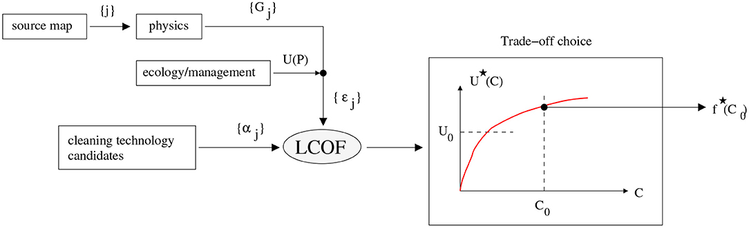
Figure 1. Information flow in the litter cleanup optimization framework (LCOF), showing the emergence of the optimal cleanup solution f^⋆ for a type 2 analysis, in this case corresponding to a given budget C₀.

2.5. Case Studies

We illustrate the cost-benefit framework above by presenting case studies in the Baltic and Mediterranean Sea, where we try to identify which sources should be prioritized for cleanup. To conduct the simplest version of the cost-benefit analysis presented above, just three quantities need to be established: (i) the time-averaged Green's function G_j(x) for considered sources j ∈ ω and (ii) an ecosystem service sensitivity P_†(x) (or relative spatial differences in this) and (iii) the cost of clean-up per weight α_j at source j. It is important to notice that time-averaged Green's functions G_j(x) may be different for different litter fractions, mainly because buoyancy leads to different vertical dynamics, different wind drag, and fractions experience different sinking rates. If this is important within the overall accuracy of the calculation, a weighted average of Green's functions for different fractions can be used for G_j(x). The Green's functions G_j(x) can be computed by either Lagrangian or Eulerian techniques, ideally giving the same results if physical processes are represented correspondingly, and using the same operational circulation models of water currents. Slightly different simulation periods apply to the Baltic and Mediterranean case studies, because different physical models were applied, but this is ignored in the analysis because we are not concerned with interannual differences in this presentation and further multiannual averages are applied both for the Baltic and Mediterranean case studies.

2.5.1. Baltic Sea Physical Model

The physical data used in the Baltic transport simulations are produced by using a Baltic-North Sea ocean-ice model HBM (HIROMB-BOOS Model) in the operational setup by the Danish Meteorological Institute (DMI). The model has been jointly developed by the HBM consortium and used as an operational model in Denmark, Estonia, Finland, and Germany. HBM is a three-dimensional, free-surface, baroclinic ocean circulation and sea ice model that solves the primitive equations for horizontal momentum and mass, and budget equations for salinity and heat on a spherical grid. The vertical transport assumes hydrostatic balance and incompressibility of sea water. Horizontal advection is modeled using a flux corrected transport scheme. The Boussinesq approximation is applied. Higher order contributions to the dynamics are parameterized following Smagorinsky (1963) in the horizontal direction and a k-ω turbulence closure scheme, which has been extended for buoyancy-affected geophysical flows in the vertical direction (Berg and Poulsen, 2012; Poulsen and Berg, 2012). The model allows for fully two-way nesting of grids with different vertical, horizontal and time resolutions, which is used to resolve narrow straits and channels. The numerical model implementation uses a staggered Arakawa C-grid and z-level coordinates and free-slip conditions along the coastlines. With two-way dynamical nesting, HBM enables high resolution in regional seas and very high resolution in narrow straits and channels. With its support for both distributed and shared memory parallelization, HBM has matured as an efficient and portable, high quality ocean model code. The HBM setup for the present hydrographic dataset has a horizontal grid spacing of 6 nautical miles (nm) in the North Sea and in the Baltic Sea, and 1 nm in the inner Danish waters. In the vertical the model has up to 50 levels in the North Sea and the Baltic Sea, and 52 levels in the inner Danish waters with a top layer thickness of 2 m. HBM is forced by DMI-HIRLAM with 10 m wind fields, sea level pressure, 2 m temperature and humidity and cloud cover. At open model boundaries between Scotland and Norway and in the English Channel, tides composed of the 8 major constituents and pre-calculated surges from a barotropic model of North Atlantic (Dick et al., 2001) are applied. Other variables are set to monthly climatological values. Freshwater runoff from the 79 major rivers in the region is obtained from a mixture of observations, climatology (North Sea rivers) and hydrological models (Baltic Sea). At the surface the model is forced with atmospheric data from the numerical weather prediction model HIRLAM (Petersen et al., 2012). The HBM setup performance has been validated on several occasions, (e.g., She et al., 2007a,b; Maar et al., 2011; Berg and Poulsen, 2012; Wan et al., 2012; Schmith and Borch, 2013). The HBM model is validated on annual basis as DMI's operational storm surge model. It has been extensively validated as CMEMS Baltic marine Forecasting model until 2020 (She, 2014) and as operational model for coastal applications (Murawski et al., 2021).

2.5.2. Baltic Sea Macro Litter Transport Model

The continuous litter distributions necessary to define Green's functions in Equation (1) were generated by averaging Lagrangian ensembles over a 10 km scale (corresponding to the scale of the hydrodynamic model applied). The quasi equilibrium litter distribution was generated by the DRRS scheme (Christensen et al., under review) from 5 year simulations, with first year as spin-up time from a uniform initial litter distribution, and the last 4 years for generating average distributions, which allows us to resolve the absolute litter density from the Lagrangian ensembles, given influx source data. Results are not sensitive to increasing the spin-up time. The DRRS scheme was setup in the modular Lagrangian framework IBMlib, which has been used in numerous studies of physical-biological interactions (Christensen et al., 2018), many of which have been conducted in the North Sea / Baltic ecoregion. IBMlib has been coupled offline to the HBM model described above, stored as hindcast database with 10 km horizontal resolution, 1 h temporal resolution, and 50 vertical layers z-grid configuration. All major physical processes recognized to be important for horizontal and vertical transport of visible plastics are included in the Baltic: Advection by ocean currents, obtained from the HBM model described above, and Stokes drift from the ECMWF ERA5 (Hersbach et al., 2020) coupled atmospheric and ocean wave model (WAM, Janssen, 2002) reanalysis with 1 h time resolution. Wind drag on low-density plastic objects are parameterized following (Yoon et al., 2010); scaling analysis for wind-driven velocity component u_w gives

$\begin{array}{ll}{u}_w~k_0\sqrt{A_a/A_w}{u}_{10}~k_0\sqrt{\frac{{\rho }_w}{{\rho }_p}-1}{u}_{10}=k{u}_{10}& (15)\end{array}$

where u₁₀ is the 10 meter air velocity vector, obtained as ECMWF ERA5 atmospheric reanalysis with 1h time resolution. A_a is the are area perpendicular to the wind direction of the plastic object above the sea surface, and A_w the area below the sea surface; ρ_w, ρ_p are the densities of water and plastic, respectively, and k₀ is a heuristic shape factor of order 0.03 (Yoon et al., 2010), consistent with Maximenko et al. (2018), expressing the ratio between above/below surface drag coefficients and air/water density as well as effective wind vertical profile near the sea surface. In addition to this comes surface layer wind drag, which in hydrodynamic models is averaged over upper grid cells; however floating plastics experience only the skin layer, and it is estimated that this is 4% of u₁₀ above the layer vertical average (Christensen et al., under review) based on a log-scaling estimate, which is added to the windage term. For simplicity we assume the area above (A_a) and below (A_w) the sea surface being equal. Consequently in the present baseline runs, we apply k = 0.07, representing pure windage and correction for finite upper layer thickness in the circulation model, in good agreement with Yoon et al. (2010) who estimated the relevant windage range to be 0 ≤ k < 0.3, and (Neumann et al., 2014) who found a good match with data when applying k ~ 0.05.

The HBM database does not contain dynamic values of vertical and horizontal sub-grid scale diffusion, so a representative horizontal diffusivity coefficient D_h of 100 m²/s is assumed as the baseline value (Gurney et al., 2001). Sinking processes are removing plastic objects from the water column. Even though progresses have been made in resolving spatio-temporal dynamics of the sinking rate λ (Kooi et al., 2017), uncertainty is too high and baseline simulations are conducted using constant representative values of λ = 0.003 day⁻¹. Retention and reactivation(resuspension) at coastlines are opposite processes that eventually reach a dynamical equilibrium, so that rates are equal and opposite when averaged over medium to long time scales. Both processes are currently not well-parameterized and subject to ongoing research. In order not to introduce additional uncertain submodels without strong observational support, it is assumed that the dynamical equilibrium between retention and reactivation also apply at short time scales for Baltic macro litter simulations; technically this implies that reflective boundary conditions applies along coastlines to incoming litter. In Christensen et al. (under review), we validate the model performance in detail, and the baseline predicts major trends in beach litter data with r = 0.49, assuming the same beaching affinity along the coastline.

2.5.3. Mediterranean Physical Model

The hydrodynamic model is based on the Princeton Ocean Model (Blumberg and Mellor, 1983) that is currently operational within the POSEIDON forecasting system (Korres et al., 2007). POM is a three-dimensional, sigma-coordinate, free surface, primitive equation model. Vertical eddy viscosity and diffusivity coefficients are calculated using the Mellor-Yamada 2.5 turbulence closure scheme (Mellor and Yamada, 1982), while horizontal diffusion is parameterized following Smagorinsky (1963) formulation. A Hybrid ensemble data assimilation algorithm (Tsiaras et al., 2017) was implemented for the assimilation of satellite altimetry and sea surface temperature data, obtained from the European Copernicus data base. The atmospheric forcing was obtained from the POSEIDON operational weather forecast (Papadopoulos et al., 2002). The waves forcing (Stokes drift, wave period and significant height), used in the Lagrangian drift model was obtained off-line from Copernicus marine service and is based on WAM Cycle 4.5.4 wave model (Günther and Behrens, 2012) that is also a component of POSEIDON forecasting system that is also a component of POSEIDON forecasting system (Ravdas et al., 2018).

2.5.4. Mediterranean Macro Litter Transport Model

The Lagrangian drift model is based on Pollani et al. (2001) and evaluates the particles' displacement taking into account of the most important processes, such as advection from ocean currents, Stokes drift from waves, particles buoyancy/sinking, random movement in the horizontal/vertical and beaching. The model follows the concept of Super-Individuals (SI—Scheffer et al., 1995) for computational efficiency, with each SI representing a group of particles, sharing the same attributes (position, weight, origin, type of plastic etc.). For macroplastics (>5 mm), which is the focus of this study, the following types/sizes were considered: 5 mm–2 cm, 2–20 cm, >20 cm bottles, >20 cm bags, >20 cm foam. A uniform background initial concentration was adopted for each type/size class, based on the basin average from available in situ data (see Tsiaras et al., 2021). New SIs are created daily from source inputs. In order to prevent the SIs total number from continuously increasing, when this exceeds a certain limit ( 2 × 10⁶), SIs of the same size/type within a predefined distance are merged and their properties averaged. The position of every SI is described by its coordinates (x, y, z) in a Cartesian system, which are updated every time-step using the 3-D displacement, produced by currents, wave and wind, obtained with bi-linear interpolation at the SI location. The Stokes drift from waves is obtained (off-line) from the wave model output and is assumed to decrease exponentially with depth. Random movement in the horizontal depends on the horizontal diffusion, obtained from the hydrodynamic model. Random movement in the vertical is assumed to depend on the vertical turbulent diffusion, obtained from the hydrodynamic model and mixing induced from waves that decays exponentially with depth. The wind drag that is practically effective only for macroplastics >20 cm (bottles, foam) is assumed to depend on the particle surface above water, following Yoon et al. (2010) parameterization Equation (15). Bottles are assumed to randomly lose their buoyancy and sink after on average 2 months floating, based on their often higher density when filled with water and in situ observations, showing a relatively small contribution of bottles in open sea floating plastics. Plastic bags that are considered as thin films (typical thickness ~ 25 μm), being prone to sinking (Chubarenko et al., 2016), along with particles with size 5 mm–2 cm and 2–20 cm are assumed to gradually lose their buoyancy from the attachment of micro- and macrofouling communities (Ye and Andrady, 1991; Fazey and Ryan, 2016) after 3, 4, and 5 months, respectively. These flotation periods corresponds to λ ~ 0.008 1/day, which is slightly higher than the level applied for the Baltic. Particles that end-up on land are assumed to remain on the beach for a fixed retention time, after which they return to the sea. During their time on the beach, the particles concentration is decreased, assuming some loss rate (e.g., burial). This is the main loss term in the model (along with sinking) and has been tuned so that the mean basin scale concentration remains fairly stable throughout the interannual simulation, obtaining also a better fit of simulated macroplastics concentration with in situ data (see Tsiaras et al., this issue).

2.5.5. Litter Sources Targeted for Cleanup and Cleanup Technologies

Riverine and beach sources of micro and macro plastic have been mapped for the Baltic and Mediterranean seas in the CLAIM Project (2021) project. In the Baltic we focus on the major rivers Oder, Nemunas, Narva, Wisla, Luga, and Daugava for the purpose of illustrating a cost-benefit assessment scenario, but other sources could be chosen as well. River sources of macroplastic to the Baltic Sea are shown in Figure 2. River source maps were obtained as an empirical function of accumulated plastics production and monthly river runoff, based on Lebreton et al. (2017) global dataset. The river input of macroplastics ( 0.7 of total microplastics+macroplastics) in the Mediterranean is shown in Figure 3. Here we focus on the effect of cleanup of the rivers Nile, Karasu, Soumman, Po, Buyuk, Seman, and Axios, which are among the major sources of plastics in the Mediterranean Sea. Several matured cleanup technologies are available commercially for macro plastic capture and removal from river sources. The Seabin device (Seabin, 2021) is a simple filtration unit that collects litter using tidal motion and a small pump; Seabin devices are placed at tactical places with easy operational access; the solution has a local fetch area, i.e., does not offer complete cleanup, but is a scalable solution. The basic unit operation cost is 2.65 € per day collecting ~ 1.5 kg of debris per day, i.e., α ~ 1.8 €/kg. A related technology is the trash wheel, as prototyped by Baltimore's Mr. Trash Wheel (Lindquist, 2016). A river current powers a large wheel lifting debris from the water and depositing it into an attached dumpster barge. The operation cost is 430 €/day removing on average 472 kg/day, i.e., α ~ 0.9 €/kg. Alternatively a non-stationary but littoral, technology like the SeaVax Robotic Vacuum Ship (SeaVax, 2015) offers more flexible cleanup deployment at 1.2 €/kg. This indicates that the cleanup price baseline is currently 1-2 €/kg. Since these technologies are based on local filtering, the price α(f) is assumed to be convex and will thus increase when scaling up toward full cleanup (f = 1); initially, we disregard this feature, and we apply an indicative marginal cleanup cost of α = 1 €/kg, reflecting a current apparent break-even level of α ~ 1 − 2 €/kg. In relation the present cost-benefit framework, the actual cleanup technologies considered need not be specified, just their equivalent cost-efficiency curves α(f), or just an average value for initial explorations.

FIGURE 2

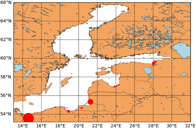
Figure 2. River sources of macroplastic inflow to the Baltic west of 13 °E; circle diameter is scaled according to yearly influx. The largest river source is Oder in the lower left corner corresponding to 67.2 tons/year.

FIGURE 3

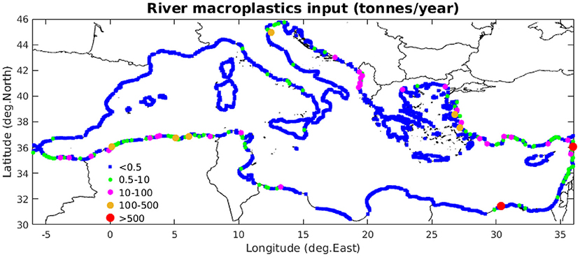
Figure 3. River sources of macroplastic inflow to the Mediterranean Sea.

2.5.6. Ecosystem Cleanup Objectives

Our understanding of the ecosystem impacts from micro and macro litter is currently not well-developed; for type 1 problems this is needed to set scientfically based management targets and for type 2 problems to parameterize the ecosystem functioning U(f). It is important to stress that the unit (e.g., biodiversity, vital rates or fishing value) of the cleanup objective U in Equation (8) does not affect the analysis; further, if the simplest functional form Equation (3) is applied, only the relative differences in litter concentration tolerance P_†(x) needs to be specified, and difficult cross sectoral and ethical discussions about the inclusion of ecosystems in anthropocentric utility functions in neo-classical welfare economics can be avoided about the explicit form of U(P) can be avoided. Previous work has used primary productivity derived from remote sensing data as a proxy for ecosystem sensitivity (Sherman and van Sebille, 2016) assuming that the latter scales with trophic flux irrespective of season. Alternatively direct maps of ichthyoplakton, zooplankton and higher trophic levels based on data synthesis are becoming increasingly available, (e.g., Beauchard et al., 2017; Beauchard and Troupin, 2018b). A consistent demonstration was suggested by the HELCOM Baltic Sea Impact Index (Halpern et al., 2008; Korpinen et al., 2010, 2012), which combines such species maps with a sensitivity matrix, based mainly on expert knowledge. Another important sensitivity map is that of the vulnerability of benthic ecosystems to sunken marine litter (Beauchard and Troupin, 2018a), which should be overlayed with the sinking flux F(x) = λ(x) P(x) that is an important auxiliary output from Eulerian/Lagrangian transport calculations. To cut the discussion short on exact weighting of different ecosystem layers, we will apply a transparent middleway by applying Natura2000 areas as sensitive areas, see Figures 4, 5, which displays original MPA (Marine Protected Area) designations (obtained in ESRI shapefile format). For type 1, the target applied will be a certain pollution reduction level, compared to present conditions; alternatives could be a certain absolute pollution level for all sensitive areas. For type 1 optimization, a pollution assessment grid were generated by projecting MPA areas in Figures 4, 5 onto the same grid applied for hydrodynamic data generation in each basin, (at native 10 and 5 km resolution, respectively) to monitor the level of cleanup obtained by a given cleanup effort f; the Baltic grid contains 280 monitoring points, the Mediterranean 2918 monitoring points. For type 2 optimization, the simplest representation of the ecosystem benefit function (Equation 3) is integrated over the full Natura 2000 networks in each sea. Results will be qualitatively independent of the particular choice of ecosystem sensitivity P_†, as the same value is assumed to apply to all sites in the network.

FIGURE 4

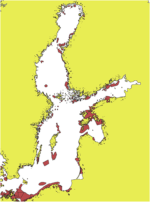
Figure 4. Baltic region Natura2000 sites. Provided by HELCOM (2021).

FIGURE 5

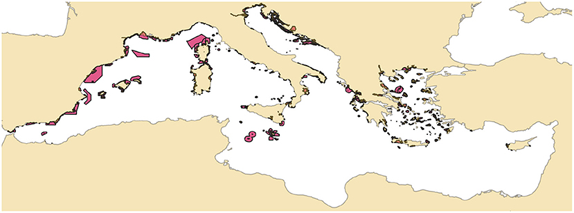
Figure 5. Mediterranean Natura2000 sites indicated by purple. Data provided by MAPAMED (2020).

3. Results

3.1. Macro Plastic Distribution and Green's Functions

Figure 6 show the average macro plastic concentration and the Green's functions for two major rivers connecting to the Baltic Sea, corresponding to a 4 year simulation period 2009–2012, with 2008 as spin-up period. The average macro plastic distribution shows enhanced abundance in near-coastal regions, especially at the Eastern side, which is likely explained by wind drag and prevailing westerly winds in the region. The temporal RMS of fluctuations around the average level in Figure 6A is large, typically 2–5 times the average, and the temporal dynamics are characterized by a varying abundance of plastics, traveling as wave patterns around in the Baltic Sea according to variable wind and current patterns; underlying transport dynamics are elaborated in more detail in Christensen et al. (under review). The Green's functions for the major rivers Oder and Narva in Figure 6 clearly show that the area of influence for sources may be very different; the Oder pollutes the most of the Baltic Sea, and most heavily the southern and Eastern Baltic regions, whereas Narva mostly affects the Gulf of Finland and the Bothnian Sea. Notice that the Greens's functions are normalized per source influx so that the plot does not show the absolute concentration of the pollution plumes.

FIGURE 6

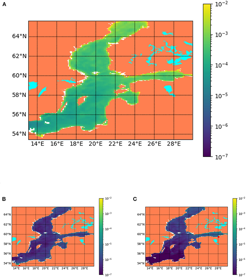
Figure 6. (A) Average macro plastic concentration in the Baltic Sea (tons/km²), corresponding to inputs from all 402 larger river sources and coast litter sources. Macro plastic Green's functions (year/km²) for (B) river Oder and (C) river Narva, corresponding to unit influx S. River mouths indicated by red circle. All distributions are generated as 4 year averages with 1 spin-up year using the DRRS equilibration scheme.

In Figure 7, the mean (2016-2018) simulated distribution of macroplastics (total from all sizes) for the Mediterranean is shown. This is primarily affected by the major sources distribution (see Figure 3), being higher in coastal areas with important source inputs (Algerian coasts, Italian and Albanian coasts in the Adriatic, Turkish coasts in the Eastern Aegean and Eastern Levantine coast). It is also affected by near surface circulation, resulting in the off-shore advection of floating plastics from coastal regions, such as the northward spread from the meandering Algerian current and the convergence of plastics in areas characterized by anticyclonic circulation, such as the Gulf of Syrte. The effect from wind/wave drift with a predominant southeast direction is mainly identified by the lower concentrations “shadows” near “protected” coasts and also the relatively lower concentration in the Aegean due to Etesian winds and the G. Lion due to the strong off-shore advection of floating particles from Mistral winds. The impact of circulation and wind/wave is also illustrated by the Green's functions calculated contribution from specific sources (Figure 7). The one for the River Soumman (Algeria) for example shows a very extended spread that covers almost the entire Western Mediterranean and reaches the Eastern Levantine following the pathway of Atlantic-Ionian stream. Another example is the River Seman (Albania) that shows an important influence throughout the Eastern Mediterranean, despite its relatively lower plastics load, compared with other major sources. It should be noted that certain Mediterranean Green's functions are essentially zero in some parts of the Mediterranean Sea so the pollution connectivity is more sparse in the Mediterranean, compared to the Baltic Sea. Also the relative differences in the Green's function range seem larger in the Mediterranean than in the Baltic Sea.

FIGURE 7

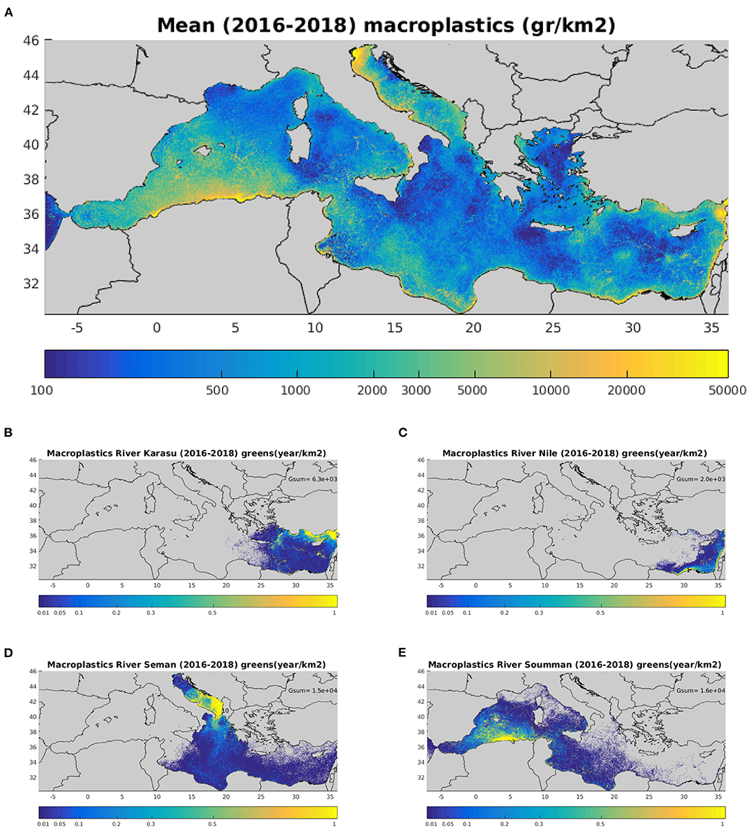
Figure 7. (A) Average macro plastic concentration in the Mediterranean Sea. (B–E) 4 examples of river source Green's functions for the Mediterranean Sea, for rivers Soumman (river mouth Algier), Seman (river mouth Albania), Nile (river mouth Egypt), Karasu (river mouth Turkey). All distributions are generated as 3 year averages.

Table 1 gives ϵ_i (Equation 5), generated with P_† = 1 inside Natura 2000 sites, and zero outside; the relative ranking of rivers and hence the optimal cleanup solution is invariant with respect to the level of P_†, since only the ratios matter. We see that ϵ_i does not correlate strictly with influx S_i, neither in the Baltic nor in the Mediterranean Sea, so that in some case it pays off to clean some smaller rivers before larger rivers, because they affect sensitive areas more per unit influx. Table 1 also reveals noticeable differences between the Baltic and Mediterranean case: the average level of ϵ appears smaller for the Mediterranean than the Baltic. This may partially be explained by different submodels for the sinking rate and beaching of macro plastic in the two implementations. It should be noted that only the relative difference influence the cost-benefit analysis, not absolute levels. However, the relative spread in ϵ also appears larger in the Mediterranean, which is more likely a feature related to hydrodynamic differences, as sources that lie in the pathway. of strong coastal currents (e.g., River Soumman, River Seman) appear to have a more extended influence (see Figure 7). For the Baltic rivers Daugava, Oder, Nemunas, Wisla give relatively similar ecological benefit per investment in plastics clean up, with a significant gap down to rivers Narva and Luga.

TABLE 1

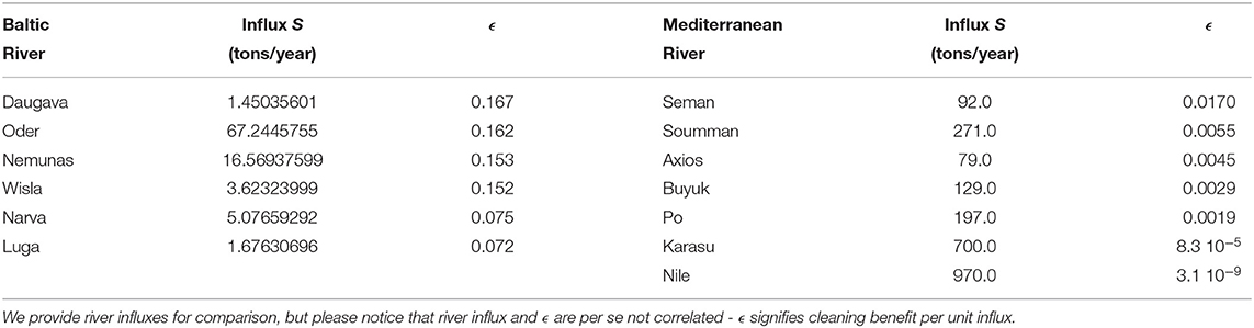
Table 1. ϵ for major rivers supplying the Baltic and Mediterranean Sea with fresh water and macro plastic pollution; rows for each region sorted according to ϵ, generated with P_† = 1 for comparison.

3.2. Cost-Benefit Analyses of Cleanup Effort Prioritization

Before embarking on the cost-benefit analysis, it is important to assess the feasibility of cleanup (Equation 2) for type 1 (fixed target) analyses, given the set of sources ω in Table 1 considered for cleanup. Here it turns out that the regional cleanup scope is more limited in the Mediterranean than for the Baltic case, see Figure 8, which shows the histogram of maximum cleanup potential ΔP/P₀ in Natura 2000 sites in both the Baltic and Mediterranean Seas. The underlying reason for this is that Mediterranean Green's functions (Figure 7) are more localized on a basin scale, compared to the Baltic Sea, which is seven times smaller areawise than the Mediterranean Sea. Also many MPAs are found in the Northwestern Mediterranean, where river pollution is particularly low, according to the adopted (Lebreton et al., 2017) dataset; further source mapping suggests that river pollution accounts for a relatively smaller fraction of the macrolitter input in the Mediterranean Sea. Actually, it turns out that 23% of the Natura 2000 areas in Figure 5 are only marginally affected by river pollution from Mediterranean rivers in Table 1, and therefore environmental conditions for this 23% of the Natura 2000 areas can consequently not be amended by cleanup of these sources. Albania, Algeria, Egypt and Turkey have national MPAs, which are not part of the Mediterranean Natura 2000 network, and these should of course be included in a realistic and more comprehensive application. For type 1 analyses, we therefore exclude these MPAs from the cleanup target, where cleanup to a specific target is infeasible by construction (Equation 2) due to prevailing transport patterns (but MPAs still benefit from cleanup); here the initial message from the analysis is that additional sources need to be considered, in order to have a higher cleanup potential at basin-scale, and this situation is expected to be occurring in other cases as well (the Baltic case also displayed a feasibility limit, but this was much higher than for the Mediterranean case).

FIGURE 8

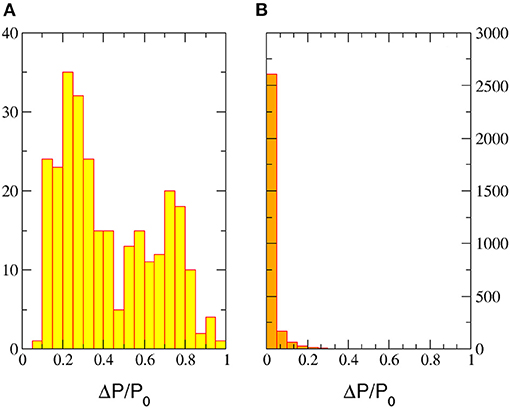
Figure 8. Histogram of primary feasibility of cleanup by Equation (2) monitored at regularly spaced sampling points within Natura 2000 sites when (A) cleanup rivers Oder, Nemunas, Narva, Wisla, Luga, and Daugava in the Baltic Sea (monitored at 280 points), and (B) cleanup rivers Nile, Karasu, Soumman, Po, Buyuk, Seman, and Axios in the Mediterranean Sea (monitored at 2,918 points).

Figure 9 illustrates the outcome of cleanup optimization in the Baltic Sea, when considering the set of pollution sources in Table 1. Figure 9A show a histogram of macro litter density within the Natura 2000 Baltic network, which is the cleanup target used for the purpose of illustration, as described above. The litter density is very variable and spans four orders of magnitude, indicating the presence of hot spots/zones. Accumulation patterns are driven by the interplay between surface currents, Stokes drift, wind drag, and coastal confinement on the other side, and is analyzed in more detail in Christensen et al. (under review). The distribution tail is slightly skewed toward the high end in the log-histogram, but the distribution is close to log-normal. Figure 9B illustrate the overall benefit of cleanup at a given cost in the Baltic Natura 2000 network by type 1/2 prioritization. The optimizations corresponds to the simplest setting with constant α(f) and linear U(P) (Equation 3), optimizing over how to distribute cleanup efforts f_j between the six considered river sources in Table 1. For type 1 analysis we consider pollution reduction factors up to 25% within each Natura2000 MPA, minimizing the cost at each reduction factor 0–25%, and then evaluating the corresponding overall ecosystem benefit at that reduction level; for each pollution reduction factor this generates a corresponding (cost, benefit) point, and the curve spans from 0 up to max 25% removed pollution (right end point). If the reduction factor is increased further the optimization problem becomes increasingly infeasible (no solution), because areas in the Natura 2000 network are also significantly influenced by other sources not considered for cleanup, which sets the upper bound for the attainable cleanup level. In this particular case, the maximum global reduction level is 8%, limited by an MPA site north of Rügen; most other points on the MPA assessment grid can attribute 20–60% of their macrolitter pollution from these six river sources. For the type 1 analysis, MPA sites that can not be cleaned up to 25% were released from the target (but still benefit from cleanup). To achieve higher reduction levels, additional sources must be considered for cleanup. For type 2, the U₂(c) curve is generated by optimizing the overall ecosystem benefit at a given cost level c, using the same cost range as the type 1 curve for comparison. Both curves U₁ and U₂ are strictly piece-wise linear in the simplest setting with constant α(f) and linear U(P). Generally U₁(c) ≤ U₂(c) since U₂ is directly maximized at a given cost level c. The underlying reason is that from an overall perspective, certain MPAs have to be over-cleaned to reach a certain pollution reduction everywhere. The type 1 and 2 curves eventually have the same right end point, corresponding to f = 1, if Green's functions are non-vanishing everywhere at monitoring points x_k. Figure 9C shows the optimizing solution for both the type 1 and 2 problem, at different cost levels. We see that the type 1 and 2 problems actually lead to rather different cleanup solution f at similar cost, even though the level of overall sub optimality type 1 is limited (Figure 9B). The type 1 optimizer f obtained by linear programming (Equation 9) has many more kinks (slope discontinuities) connected by linear segments compared to the type 2 optimizer, which also comes from linear programming, where sources are cleaned fully in successive order according to the ranking principle (Equation 13).

FIGURE 9

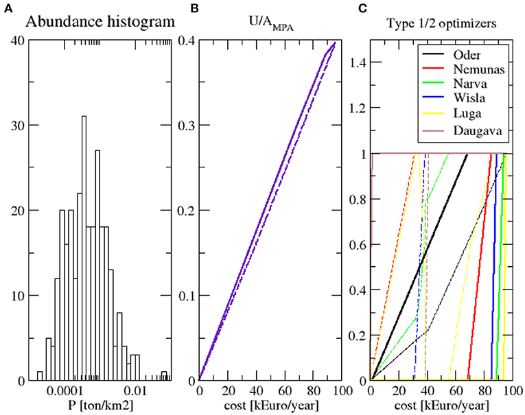
Figure 9. (A) Histogram of average Baltic macro plastic density on assessment grid within Natura 2000 MPAs in Figure 4. (B) MPA integrated benefit of cleanup per area U/A_MPA as function of cost for fixed-objective (type 1, dashed line) or best-value-per-cost (type 2, full line). End point on dashed curve correspond to at least 25% local pollution reduction at all feasible points on assessment grid. For the plot we applied P_† = < P >_MPA so BAU reference scenario (f = 0) corresponds to U/A_MPA = 0 and full cleanup (P(x) = 0) of all sources (also beyond 6 river in Table 1 corresponds to U/A_MPA = 1 (C) Cost-minimizing solution f for different river sources in Table 1 corresponding to B) for type 1 optimization (dashed curves) and type 2 optimization (full curves).

In Figure 10, the corresponding cost benefit analysis for the source cleanup benefiting the Mediterranean Natura 2000 MPAs in Figure 5 is shown, when considering the set of pollution sources in Table 1. Figure 10A shows a histogram of macro litter density within the MPAs. As for the Baltic Sea, the litter density is very variable and spans five orders of magnitude, again indicating the presence of hot spots/zones; on average the pollution level is about 20% higher compared to the Baltic, but the exact number will be sensitive to sink parameterization. The Mediterranean is a semi-enclosed basin that is considered a hot-spot of plastic pollution (Suaria and Aliani, 2014), resulting from its densely populated coastline and the limited outflow of surface waters. The density distribution is more symmetric compared to the Baltic in Figure 9A, so it is closer to a log-normal distribution.

FIGURE 10

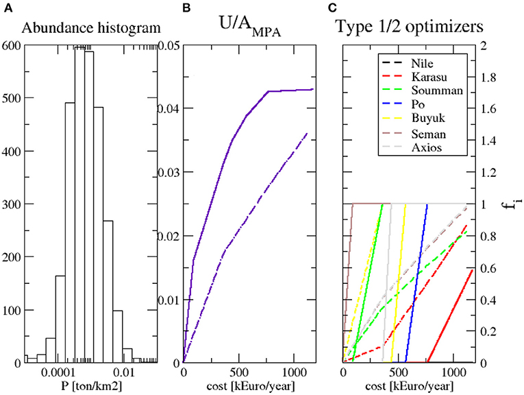
Figure 10. (A) Histogram of average Mediterranean macro plastic density on assessment grid within Natura 2000 MPAs in Figure 5. (B) MPA integrated benefit of cleanup per area U/A_MPA as function of cost for fixed-objective (type 1, dashed line) or best-value-per-cost (type 2, full line). End point on dashed curve correspond to at least 10% local pollution reduction at all feasible points on assessment grid. For the plot we applied P_† = < P >_MPA so BAU reference scenario (f = 0) corresponds to U/A_MPA = 0 and full cleanup (P(x) = 0) of all sources (also beyond 6 river in Table 1 corresponds to U/A_MPA = 1 (C) Cost-minimizing solution f for different river sources in Table 1 corresponding to B) for type 1 optimization (dashed curves) and type 2 optimization (full curves).

Figure 10B illustrate the overall benefit of cleanup at a given cost in the Mediterranean Natura 2000 network by type 1/2 prioritization. As before the optimizations corresponds to the simplest setting with constant α(f) and linear U(P) (Equation 3), optimizing over how to distribute the cleanup effort f between the seven river sources considered in Table 1. Again for type 1 analysis, the curve is generated by increasing the required pollution reduction factor, minimizing the cost at that reduction factor, and evaluating the overall ecosystem benefit; for the Mediterranean Sea we consider an up to 10% pollution reduction in the MPA areas by cleaning up the 7 rivers, and for each pollution reduction factor this generates a corresponding (cost, benefit) point, and the curve spans from 0 up to max 10% removed pollution (right end point). If the reduction factor is increased to higher levels, the optimization problem becomes increasingly infeasible (no solution), with fewer MPA sites being able to reach the target. For type 2, the U₂(c) curve is generated by optimizing the overall ecosystem benefit at a given cost level c, at a set of cost levels corresponding to the type 1 curve for comparison. Both curves U₁ and U₂ are strictly piece-wise linear in the simplest setting with constant α(f) and linear U(P), but in this case U₂ appears overall more concave than U₂ for the Baltic Sea, and type 2 (overall) cost-benefit optimization gives more value for the cleanup investment.

4. Discussion

In this paper, we presented a consistent framework for cost-benefit analysis of marine litter cleanup. Because it is based on first principles, it allows for systematic refinements of assumptions and approximations. The simplest setting was applied for the Baltic and Mediterranean case studies and below we outline the major assumptions and approximations, their influence and potential pathways for amendment. The pollution sources and study areas chosen in this paper are not special and we expect our framework to be applicable to other coastal regions as well if the corresponding input data is supplied. In relation to a particular target it is important that the considered set of rivers are relevant and carry a significant fraction of the input. This is checked by the feasibility analysis (Equation 2) In Christensen et al. (under review), we give a more detailed account of major knowledge gaps and uncertainties in relation to the physics (transport simulations) applied for computing Green's functions.

Different macro litter fractions display different dispersal patterns away from the source; this is mainly due to different experienced wind drag k, caused by buoyancy differences and differences in size and shape, but wave interaction may also play a significant role. It has already been pointed out that this has the potential to create spatial litter stratification by windage (Maximenko et al., 2018), which would constitute a rich validation data set. Additionally the sinking rate λ(x, t) determines the extend of the Green's function and will depend mainly on buoyancy and size of the objects, as well as seasonal and spatial differences in biofouling rate, which also depend of material and surface texture.

To confine uncertainty in transport simulations it is necessary to know the composition of the litter from sources, expressed as a statistical distribution over (k, λ) (as a first approximation). This is akin to the new trait-based paradigm in ecology, where the analysis focuses on key traits rather than individual species (Kiørboe et al., 2018). The idea of considering low-dimensional statistical distributions of litter types, rather than arbitrary more or less representative selections of specific litter pieces has already been suggested by Kooi and Koelmans (2019), which suggested size, Corey shape factor and density as pragmatic covariates for the statistical distributions; our work suggests that the most relevant covariates aligned with a modeling perspective are (k, λ), which are more complicated to measure routinely, so that an important future research issue is linkage functions from easily measurable litter attributes to (k, λ), and identifying easily measurable litter attributes in addition to size, shape and density that determine (k, λ), like surface texture. Such input is important to standardize the sampling methodology and reporting practices for detection, quantification, and characterization of plastic debris in the marine environment, which is currently critically lacking (Law, 2017).

Then, by linearity of transport, the effective Green's function is just the G_{k, λ} weighted by the statistical distribution over (k, λ) of litter. If the ecological impact of different macro litter fractions are comparable, the cost-benefit analysis may be conducted using the obtained effective Green's function, alternatively different representative fractions must be accounted for in parallel, extending the set of sources ω in the analysis. Assessing the statistical distribution over (k, λ) of marine litter today is far beyond survey recording practices, where observational categories are very coarse, disjoint and aimed at low-effort postprocessing, e.g., “plastic,” “plastic < 5 cm.” As a minimum, to allow data-pooling and meta-studies, a common set of observational categories needs to be established, preferably a hierarchical system as applied for habitat classification (Davies and Moss, 2000, 2004). The approach until now has not addressed that plastic litter possibly break up before eventually sinking. Breakup products will disperse independently. If fragments keep (k, λ) corresponding to the parent, the result will be the same, because Lagrangian/Eulerian simulations have a diffusive term representing the effect of sub-scale eddies statistically. According to Kooi et al. (2017) this is likely not the case for λ, and due to the air flow profile vertical scaling near the sea surface, it is likely not the case for k either. So studying the temporal dynamics of a distribution over (k, λ) is of interest, also to address the long-term fate of marine litter.

In the current formulation cleanup at sources is assumed, which is expected to be most effective from an entropic point of view, and also supported by pilot studies (Sherman and van Sebille, 2016), however, off-shore cleanup is also conceivable as for example add-on installations at wind farms. It can be shown that the Green's function technique advanced in this work can also be extended to cover off-source cleanup, thus allowing to cross-compare a wider palette of cleanup alternatives in an integrated framework.

Case studies were developed using the simple relation Equation (3) for type 2 analyses of ecosystem impact. Even though the biological literature is equivocal on the adverse effect and potential dangers of marine plastic, evidence is qualitative and categorical (e.g., statistics of species having detectable interaction with unmanaged plastic), and collected data are usually habitat and species specific. In light of the complexity of physiological processes leading to vital rates, the literature today falls short of mapping ecosystem functioning directly to the continuous litter density, and in this perspective it becomes an academic exercise to go far beyond the simplicity of Equation (3). If the underlying ecosystem functioning really respond non-linearly to plastic abundance (as opposed to gradually linear as in Equation (3)), the next observational step would be to seek a step function, which also just contain one essential parameter (the sharp threshold) to be estimated. In this case, the type 1 and 2 problems become mathematically isomorphic, and need to be solved like the type 1 problem in the present formulation with very little adaptation. For the type 2 formulation in the present context, only the relative values of P_† are important, but with the step function, the absolute value matters.

In addition to potential non-linearity of ecosystem functioning, non-linearity of the cost function also needs to be considered. This non-linearity is more tangible and easier to assess than that of ecosystem functioning and the impacts on ecosystem service delivery (e.g., recreation, commercial fisheries etc.). The underlying reason is that for many cleanup techniques, e.g., those relying on local filtering, it progressively becomes more difficult to remove all litter which implies that c(f) becomes a convex function in cleanup degree f. In the Supplementary Materials we demonstrate that a logarithmic scaling is expected on rather generally c(f) ~ −log(1 − f)) as f → 1, if installation costs are discounted over the lifetime of the technology, so that the last term in Equation (6) becomes −α_jS_jlog(1 − f_j)). This renders the objective functions Equations (7), (8) non-linear in the interior and weakly singular at the right boundary f = 1, so the optimization problems are of the general KKT type. Generally speaking, this means the solution will be left-interior f < 1 and not be constituted by linear segments as in Figures 9C, 10C, and the convenient ranking principle for linear type 2 problems (Equation 13) will not apply strictly.

In our case studies we applied the indicative marginal cleanup cost of α = 1 €/kg as baseline in our example case studies. With the current increasing level of research and development in sustainable cleanup and recycling (see e.g., OceanCleanupProject, 2013) this baseline is expected to drop with industrial scaleup and optimization in the future; a reduced cleanup cost level α will not, however, change the approach and results outlined in this paper, but merely change the cost scale axis in figures like Figures 1, 9, 10, and allow for cleaner oceans for a given level of societal investment in cleaning.

The plastic source map applied in this work represents current best knowledge, however this data set has certain shortcomings, most importantly that the Russian sources are not available. We expect inclusion of this will lead to higher plastic concentrations in the Gulf of Finland and the Bothnian Sea. The Greens functions computed for riverine sources are insensitive to error and biases in the source map, but average plastic distribution is sensitive to errors. It is important to stress that our integrated framework will also work for an amended source map and results will be qualitatively similar, even though quantitative results may change a little reflecting updated input.

In the regional case studies we have applied a constant litter influx, corresponding to the limited available data, without seasonal patterns or short term interannual trends. However, it is not unlikely that a significant time variation is present in the influx for each source, reflecting for example precipitation dynamics, changing seasonal consumption patterns and overall economic activity level. If such submodels were available, they could be applied as modulations on the constant litter influx levels applied in the current setups. Technically this means that time varying Green's functions must be applied, but our frame work can relatively easily be extended to cover this. However, it only makes sense to consider this advancement, if also a non-linear ecosystem functioning is applied, because averaged ecosystem functioning is not the same as ecosystem functioning under averaged conditions. Another aspect calling for an extension to time varying Green's functions is vulnerable periods in the ecosystem, for instance spawning seasons. As a first step in this direction, a temporal clip may be applied when time-averaging the Green's functions. Alternatively a lower tolerance limit could be applied to the entire season, when setting targets or defining the U functions.

Related to this discussion is also the effect of short-term fluctuations in litter distribution. A first generalization of the current framework in this direction is to simulate local temporal fluctuations σ_P(x) in litter density with an equation similar to Equation (1), developed the time dependent Green's function. This allow for an amended representations of the ecosystem functioning U = U(P, σ_P).

In our presentation, we have leaned toward U representing non-monetized aspects of ecosystem functioning and ecosystem service provision. Depending on the starting point, U may also partially or fully represent an economic aspect of ecosystem functioning, e.g., fishing yield value or recreational sector revenue. From a mathematical point of view, it makes no difference in the optimization procedure whether U represents an ecological conservation aspect or a monetized utility aspect. The dilemma is partly ethical and partly methodological based on academic and policymaker confidence in available environmental valuation methods. Our framework can handle both perspectives, and the choice is visible up front in the definition of Z₂. A detailed discussion of the case where U is a monetized representation ecosystem services and functioning is beyond the scope of this manuscript. But in this case U and C have the same unit, and the natural value in Equation (8) is κ = 1 so income and costs are at same footing and the problem is a standard profit maximization problem, with f as control variables. In this case these is a risk that Z₂ looses convexity and/or the mathematical solution becomes trivial (f = 0) implying no cleanup at all.

Although beyond the scope of the present work, for type 1 (cost minimization) problems, it is relatively straight forward to include other social, political and geopolitical issues when applying a regional cleanup solution, by ad hoc adjustments of targets. It is also possible to add penalty terms (or additional inequality terms) to Equation (8). The present framework then allows to assess the degree of suboptimality—or quantify the additional cost incurred—by such constraints.

5. Conclusions

We presented a quantitative framework to optimize choices across technologies and sites for cleaning up marine litter at regional scale, and identified which cross-disciplinary input is needed to support scientifically sound marine litter cleanup strategy planning. Our formulation is a consistent first principles approach combining data from physics, biology, cleanup engineering, and economics which allows for systematic extensions. We identify two cost-benefit problem categories: cost minimization and benefit maximization, which have different objective functions and different solutions. In the simplest case with linear cleanup-cost and ecosystem functioning, the target-driven analysis leads to a robust linear programming problem. The best-value can be solved analytically by a ranking principle, in the simplest case. When more complex cleanup-cost and ecosystem functioning representations are included, the framework leads to a general KKT optimization problem. Furthermore, the integrated framework allows to test the feasibility of a given cleanup target by considering the source litter dispersal Green's functions, which was an important step, as illustrated in our two regional case studies. Best-value cleanup formulations have no feasibility constraints. The parameterization requirements in the framework is relatively benign, since in many cases only ratios or relative values of properties are needed. We present case studies of cleanup in the Baltic and Mediterranean Seas demonstrating the framework, and several interesting results emerge. Green's functions in the Mediterranean Sea appear more localized which lowers the feasibility of a given target, if a given set of river sources are considered for cleanup, and successful cleanup is more dependent on including enough sources. For both the Baltic and the Mediterranean Sea upper limits of cleanup feasibility are set by sites under influence of local pollution sources not included in the cleanup plan. In both cases it is also not most favorable to clean up the largest sources first, considering the overall ecosystem benefits. Our work has demonstrated that it is pivotal to include litter transport simulation in the planning of regional scale cleanup strategies, if ecosystem benefit are to be maximized for the resources to be invested in marine litter cleanup.

Data Availability Statement

The raw data supporting the conclusions of this article will be made available by the authors, without undue reservation.

Author Contributions

AC developed the underlying cost-benefit framework, conducted cost-benefit analyses and conducted the Baltic Sea litter simulations and initiated the manuscript. KT conducted the Mediterranean physical and litter simulations and contributed to the manuscript. JM conducted Baltic Sea physical simulations and contributed to the manuscript. YH conducted the Mediterranean physical and litter simulations and contributed to the manuscript. RB contributed to the underlying cost-benefit and cost-effectiveness analysis framework and contributed to the manuscript. JS conducted Baltic source mapping and contributed to the manuscript. MS, and RB contributed to the manuscript. All authors contributed to the article and approved the submitted version.

Funding

This work was supported by the EU Horizon2020 project (CLAIM Project, 2021) (grant agreement No. 774586).

Conflict of Interest

The authors declare that the research was conducted in the absence of any commercial or financial relationships that could be construed as a potential conflict of interest.

The reviewer PK declared a past co-authorship with one of the authors RB to the handling editor.

Publisher's Note

All claims expressed in this article are solely those of the authors and do not necessarily represent those of their affiliated organizations, or those of the publisher, the editors and the reviewers. Any product that may be evaluated in this article, or claim that may be made by its manufacturer, is not guaranteed or endorsed by the publisher.

Acknowledgments

Financial support from the Horizon2020 program is acknowledged by all authors.

References

Beauchard, O., and Troupin, C. (2018a). Distribution of Benthic Macroinvertebrate Living Modes in European Seas. Technical report, EModNet - Marine Data Archive. doi: 10.14284/373

CrossRef Full Text

Beauchard, O., and Troupin, C. (2018b). Distribution of Fish Living Modes in European Seas. Technical report, EModNet - Marine Data Archive. doi: 10.14284/374

CrossRef Full Text | Google Scholar

Beauchard, O., Verissimo, H., Queiros, A., and Herman, P. (2017). The use of multiple biological traits in marine community ecology and its potential in ecological indicator development. Ecol. Indicat. 76, 81–96. doi: 10.1016/j.ecolind.2017.01.011

CrossRef Full Text | Google Scholar

Berg, P., and Poulsen, J. W. (2012). Implementation Details for HBM. Technical report, Danish Meteorological Institute.

Google Scholar

Blumberg, A., and Mellor, G. (1983). Diagnostic and prognostic numerical circulation studies of the south atlantic bight. J. Geophys. Res. 88, 4579–4592. doi: 10.1029/JC088iC08p04579

CrossRef Full Text | Google Scholar

Boyd, S. P., and Vandenberghe, L. (2010). Convex Optimization. New York, NY: Cambridge University Press.

Google Scholar

Brouwer, R., and De Blois, C. (2008). Integrated modelling of risk and uncertainty underlying the cost and effectiveness of water quality measures. Environ. Modell. Softw. 23, 922–937. doi: 10.1016/j.envsoft.2007.10.006

CrossRef Full Text | Google Scholar

Christensen, A., Mariani, P., and Payne, M. R. (2018). A generic framework for individual-based modelling and physical-biological interaction. PLoS ONE 13:e0189956. doi: 10.1371/journal.pone.0189956

PubMed Abstract | CrossRef Full Text | Google Scholar

Chubarenko, I., Bagaev, A., Zobkov, M., and Esiukova, E. (2016). On some physical and dynamical properties of microplastic particles in marine environment. Mar. Pollut. Bull. 108, 105–112. doi: 10.1016/j.marpolbul.2016.04.048

PubMed Abstract | CrossRef Full Text | Google Scholar

CLAIM Project (2021). Cleaning Litter by Developing and Applying Innovative Methods in European Seas.

Davies, C. E., and Moss, D. (2000). “The EUNIS habitat classification,” in ICES Annual Science Conference 2000, Dorset.

Davies, C. E., and Moss, D. (2004). EUNIS Habitat Classification Marine Habitat Types: Revised Classification and Criteria. Technical report, Centre for Ecology and Hydrology, Dorset.

Google Scholar

Dick, S., Kleine, E., Müller-Navarra, S., Klein, H., and Komo, H. (2001). The Operational Circulation Model of BSH (BSHcmod) - Model Description and Validation. Technical report, Bundesamts für Seeschifffahrt und Hydrographie.

Google Scholar

Fazey, F. M., and Ryan, P. G. (2016). Biofouling on buoyant marine plastics: an experimental study into the effect of size on surface longevity. Environ. Pollut. 210, 354–360. doi: 10.1016/j.envpol.2016.01.026

PubMed Abstract | CrossRef Full Text | Google Scholar

Günther, H., and Behrens, A. (2012). The WAM Model. Validation Document Version 4.5.4. Technical report, Intitute of Coastal Research Helmholtz-Zentrum Geesthach (HZG).

Gurney, W. S. C., Speirs, D. C., Wood, S. N., Clarke, E. D., and Heath, M. R. (2001). Simulating spatially and physiologically structured populations. J. Anim. Ecol. 70, 881–894. doi: 10.1046/j.0021-8790.2001.00549.x

CrossRef Full Text | Google Scholar

Halpern, B. S., Walbridge, S., Selkoe, K. A., Kappel, C. V., Micheli, F., D'Agrosa, C., et al. (2008). A global map of human impact on marine ecosystems. Science 319, 948–952. doi: 10.1126/science.1149345

PubMed Abstract | CrossRef Full Text | Google Scholar

Hardesty, B. D., and Wilcox, C. (2017). A risk framework for tackling marine debris. Anal. Methods 9, 1429–1436. doi: 10.1039/C6AY02934E

CrossRef Full Text | Google Scholar

HELCOM (2021). Map and Data Service (HELCOM MADS). Available online at: http://maps.helcom.fi/website/mapservice/

Hersbach, H., Bell, B., Berrisford, P., Hirahara, S., Horanyi, A., Munoz-Sabater, J., et al. (2020). The ERA5 global reanalysis. Q. J. R. Meteorol. Soc. 146, 1999–2049. doi: 10.1002/qj.3803

CrossRef Full Text | Google Scholar

Janssen, P. (2002). “The wave model,” in Meteorological Training Course Lecture Series (Reading: ECMWF). Available online at: https://www.ecmwf.int/node/16951

Google Scholar

King, P. (2018). Fishing For Litter: A Cost-Benefit Analysis of How to Abate Ocean Pollution. University Library of Munich, Munich. doi: 10.2139/ssrn.3338551

CrossRef Full Text | Google Scholar

Kiørboe, T., Visser, A., and Andersen, K. H. (2018). A trait-based approach to ocean ecology. ICES J. Mar. Sci. 75, 1849–1863. doi: 10.1093/icesjms/fsy090

CrossRef Full Text | Google Scholar

Kooi, M., and Koelmans, A. A. (2019). Simplifying microplastic via continuous probability distributions for size, shape,and density. Environ. Sci. Technol. Lett. 6, 551–557. doi: 10.1021/acs.estlett.9b00379

CrossRef Full Text | Google Scholar

Kooi, M., Van Nes, E. H., Scheffer, M., and Koelmans, A. A. (2017). Ups and downs in the ocean: effects of biofouling on vertical transport of microplastics. Environ. Sci. Technol. 51, 7963–7971. doi: 10.1021/acs.est.6b04702

PubMed Abstract | CrossRef Full Text | Google Scholar

Korpinen, S., Laura Meski, J. H. A., and Laamanen, M. (2010). “Towards a tool for quantifying anthropogenic pressures and potential impacts on the baltic sea marine environment: a background document on the method, data and testing of the baltic sea pressure and impact indices,” in Baltic Sea Environmental Proceedings (Helsinki: HELCOM). Available online at: https://helcom.fi/wp-content/uploads/2019/08/BSEP125.pdf

Korpinen, S., Meski, L., Andersen, J. H., and Laamanen, M. (2012). Human pressures and their potential impact on the baltic sea ecosystem. Ecol. Indicat. 15, 105–114. doi: 10.1016/j.ecolind.2011.09.023

CrossRef Full Text | Google Scholar

Korres, G., Hoteit, I., and Triantafyllou, G. (2007). Data assimilation into a princeton ocean model of the mediterranean sea using advanced kalman filters. J. Mar. Syst. 65, 84–104. doi: 10.1016/j.jmarsys.2006.09.005

CrossRef Full Text | Google Scholar

Law, K. L. (2017). Plastics in the marine environment. Annu. Rev. Mar. Sci. 9, 205–229. doi: 10.1146/annurev-marine-010816-060409

PubMed Abstract | CrossRef Full Text | Google Scholar

Lebreton, L., van der Zwet, J., Damsteeg, J., Slat, B., Andrady, A., and Reisser, J. (2017). River plastic emissions to the world's oceans. Nat. Commun. 8:15611. doi: 10.1038/ncomms15611

PubMed Abstract | CrossRef Full Text | Google Scholar

Lebreton, L. C., Greer, S. D., and Borrero, J. C. (2012). Numerical modelling of floating debris in the world's oceans. Mar. Pollut. Bull. 64, 653–661. doi: 10.1016/j.marpolbul.2011.10.027

PubMed Abstract | CrossRef Full Text | Google Scholar

Lindquist, A. (2016). Baltimore's MR. Trash wheel. J. Ocean Technol. 11, 28–35.

Google Scholar

Maar, M., Møller, E. F., Larsen, J., Madsen, K. S., Wan, Z., She, J., et al. (2011). Ecosystem modelling across a salinity gradient from the north sea to the baltic sea. Ecol. Modell. 222, 1696–1711. doi: 10.1016/j.ecolmodel.2011.03.006

CrossRef Full Text | Google Scholar

MAPAMED (2020). The Mediterranean Marine Protected Areas Database.

Maximenko, N., Corradi, P., Law, K. L., Van Sebille, E., Garaba, S. P., Lampitt, R. S., et al. (2019). Toward the integrated marine debris observing system. Front. Mar. Sci. 6:447. doi: 10.3389/fmars.2019.00447

CrossRef Full Text | Google Scholar

Maximenko, N., Hafner, J., Kamachi, M., and MacFadyen, A. (2018). Numerical simulations of debris drift from the great japan tsunami of 2011 and their verification with observational reports. Mar. Pollut. Bull. 132, 5–25. doi: 10.1016/j.marpolbul.2018.03.056

PubMed Abstract | CrossRef Full Text | Google Scholar

Maximenko, N., Hafner, J., and Niiler, P. (2012). Pathways of marine debris derived from trajectories of lagrangian drifters. Mar. Pollut. Bull. 65, 51–62. doi: 10.1016/j.marpolbul.2011.04.016

PubMed Abstract | CrossRef Full Text | Google Scholar

McIlgorm, A., Campbell, H. F., and Rule, M. J. (2011). The economic cost and control of marine debris damage in the asia-pacific region. Ocean Coast. Manage. 54, 643–651. doi: 10.1016/j.ocecoaman.2011.05.007

CrossRef Full Text | Google Scholar

Mellor, G. L., and Yamada, T. (1982). Development of a turbulence closure model for geophysical fluid problems. Rev. Geophys. 20:851. doi: 10.1029/RG020i004p00851

CrossRef Full Text | Google Scholar

Murawski, J., She, J., Mohn, C., Frishfelds, V., and Nielsen, J. W. (2021). Ocean circulation model applications for the estuary-coastal-open sea continuum. Front. Mar. Sci. 8:657720. doi: 10.3389/fmars.2021.657720

CrossRef Full Text | Google Scholar

Neumann, D., Callies, U., and Matthies, M. (2014). Marine litter ensemble transport simulations in the southern north sea. Mar. Pollut. Bull. 86, 219–228. doi: 10.1016/j.marpolbul.2014.07.016

PubMed Abstract | CrossRef Full Text | Google Scholar

OceanCleanupProject (2013). The Ocean Cleanup.

Google Scholar

Papadopoulos, A., Katsafados, P., Kallos, G., and Nickovic, S. (2002). The weather forecasting system for poseidon - an overview. Global Atmos. Ocean Syst. 8, 219–237. doi: 10.1080/1023673029000003543

CrossRef Full Text | Google Scholar

Petersen, C., Kmit, M., Nielsen, N. W., Amstrup, B., and Huess, V. (2012). Performance of DMI-HIRLAM-T15 and DMI-HIRLAM-S05 and the Storm Surge Model in Winter Storms. Technical report, Danish Meteorological Institute.

Pollani, A., Triantafyllou, G., Petihakis, G., Konstantinos, N., Dounias, K., and Koutitas, C. (2001). The poseidon operational tool for the prediction of floating pollutant transport. Mar. Pollut. Bull. 43, 270–278. doi: 10.1016/S0025-326X(01)00080-7

PubMed Abstract | CrossRef Full Text | Google Scholar

Poulsen, J. W., and Berg, P. (2012). More Details on HBM - General Modelling Theory and Survey of Recent Studies. Technical report, Danish Meteorological Institute.

Google Scholar

Ravdas, M., Zacharioudaki, A., and Korres, G. (2018). Implementation and validation of a new operational wave forecasting system of the Mediterranean Monitoring and Forecasting Centre in the framework of the Copernicus Marine Environment Monitoring Service. Nat. Hazards Earth Syst. Sci. 18, 2675–2695. doi: 10.5194/nhess-18-2675-2018

CrossRef Full Text | Google Scholar

Scheffer, M., Baveco, J., DeAngelis, D., Rose, K., and van Nes, E. (1995). Super-individuals a simple solution for modelling large populations on an individual basis. Ecol. Modell. 80, 161–170. doi: 10.1016/0304-3800(94)00055-M

CrossRef Full Text | Google Scholar

Schmith, T., and Borch, U. (2013). Horns Rev 3 Offshore Wind Farm - Validation of DMI's Model Suite for the Horns Rev 3 Area. Technical report, Orbicon and DMI.

Seabin (2021). Seabin Project - for Cleaner Oceans.

SeaVax (2015). Sea & River Vax Project.

She, J. (2014). “Myocean baltic sea monitoring and forecasting centre, conference: operational oceanography for sustainable blue growth: the seventh EuroGOOS conference, Lisbon,” in Proceedings of the Seventh EuroGOOS Conference, eds E. Buch, Y. Antoniou, D. Eparkhina, and G. Nolan (Brussels: EuroGOOS), 33–42.

She, J., Berg, P., and Berg, J. (2007a). Bathymetry impacts on water exchange modelling through the danish straits. J. Mar. Syst. 65, 450–459. doi: 10.1016/j.jmarsys.2006.01.017

CrossRef Full Text | Google Scholar

She, J., Berg, P., Larsen, J., and Nielsen, J. W. (2007b). Operational three dimensional ocean modelling for the Baltic sea. Environ. Res. Eng. Manage. 39, 3–7.

Google Scholar

Sherman, P., and van Sebille, E. (2016). Modeling marine surface microplastic transport to assess optimal removal locations. Environ. Res. Lett. 11:014006. doi: 10.1088/1748-9326/11/1/014006

CrossRef Full Text | Google Scholar

Smagorinsky, J. (1963). General circulation experiments with the primitive equations. I. The basic experiment. Monthly Weather Rev. 91, 99–164. doi: 10.1175/1520-0493(1963)091<0099:GCEWTP>2.3.CO;2

CrossRef Full Text | Google Scholar

Suaria, G., and Aliani, S. (2014). Floating debris in the Mediterranean sea. Mar. Pollut. Bull. 86, 494–504. doi: 10.1016/j.marpolbul.2014.06.025

PubMed Abstract | CrossRef Full Text | Google Scholar

Tsiaras, K., Hatzonikolakis, Y., Kalaroni, S., Pollani, A, and Triantafyllou, G. (2021). Modeling the pathways and accumulation patterns of micro- and macro-plastics in the Mediterranean. Front. Mar. Sci. 8:743117. doi: 10.3389/fmars.2021.743117

CrossRef Full Text

Tsiaras, K., Hoteit, I., Kalaroni, S., Petihakis, G., and Triantafyllou, G. (2017). A hybrid ensemble-OI Kalman filter for efficient data assimilation into a 3-d biogeochemical model of the Mediterranean. Ocean Dyn. 67, 673–690. doi: 10.1007/s10236-017-1050-7

CrossRef Full Text | Google Scholar

Van Sebille, E., Aliani, S., Law, K. L., Maximenko, N., Alsina, J. M., Bagaev, A., et al. (2020). The physical oceanography of the transport of floating marine debris. Environ. Res. Lett. 15:023003. doi: 10.1088/1748-9326/ab6d7d

CrossRef Full Text | Google Scholar

van Sebille, E., England, M. H., and Froyland, G. (2012). Origin, dynamics and evolution of ocean garbage patches from observed surface drifters. Environ. Res. Lett. 7:044040. doi: 10.1088/1748-9326/7/4/044040

CrossRef Full Text | Google Scholar

Wan, Z., She, J., Maar, M., Jonasson, L., and Baasch-Larsen, J. (2012). Assessment of a physical-biogeochemical coupled model system for operational service in the baltic sea. Ocean Sci. 8, 683–701. doi: 10.5194/os-8-683-2012

CrossRef Full Text | Google Scholar

Ye, S., and Andrady, A. (1991). Fouling of floating plastic debris under biscayne bay exposure conditions. Mar. Pollut. Bull. 22, 608–613. doi: 10.1016/0025-326X(91)90249-R

CrossRef Full Text | Google Scholar

Yoon, J. H., Kawano, S., and Igawa, S. (2010). Modeling of marine litter drift and beaching in the Japan sea. Mar. Pollut. Bull. 60, 448–463. doi: 10.1016/j.marpolbul.2009.09.033

PubMed Abstract | CrossRef Full Text | Google Scholar

Zambianchi, E., Trani, M., and Falco, P. (2017). Lagrangian transport of marine litter in the Mediterranean sea. Front. Environ. Sci. 5:5. doi: 10.3389/fenvs.2017.00005

CrossRef Full Text | Google Scholar