 Jingxuan Wei
 Kathryn L. Gunn
 Robert Reece1
- 1Department of Geology and Geophysics, Texas A&M University, College Station, TX, United States
- 2Centre for Southern Hemisphere Oceans Research (CSHOR), CSIRO Oceans and Atmosphere, Hobart, TAS, Australia
We investigate the spatial distribution of diapycnal mixing and its drivers in the central South Atlantic thermocline between the Rio-Grande Rise to the Mid-Atlantic Ridge. Diapycnal mixing in the ocean interior influences the slowly evolving meridional circulation, yet there are few observations of its variability with space and time or its drivers. To overcome this gap, seismic reflection data are spectrally analyzed to produce a 1,600 km long full-thermocline vertical section of diapycnal diffusivity, that has a vertical and horizontal resolution of O(10) m and spans a period of 4 weeks. We compare seismic-derived diffusivities with CTD-derived diffusivities and direct observations from 1996, 2003, and 2011. In the mean and on decadal scales, we find that thermocline diffusivities have changed little in this region, retaining a background value of 1 × 10⁻⁵ m2 s–1. Imprinted upon the background rates, mixing is heterogeneous at mesoscales. Enhanced mixing, exceeding 10 × 10–5 m2 s–1 and spreading between 200 and 700 m depth, is found above the Mid-Atlantic Ridge suggesting the ridge enhances diffusivity by at least one order of magnitude across the entire water column. Rapid decay of diffusivities within 30 km of the ridge implies local dissipation of tidal energy. Above smooth topography, patches of enhanced mixing are possibly caused by a recent storm that injects near-inertial energy into the water column and elevates mixing from 3 × 10⁻⁵ m2 s–1 to 50 × 10–5 m2 s–1 down to depths of more than 600 m. The propagation speed of near-inertial energy varies substantially from 17 to 27 m/day. Faster speed, and therefore greater penetration depths of 800 m, are probably facilitated by an eddy. Together, these data extend the observational record of central South Atlantic thermocline mixing and provide insights into drivers of mesoscale variability.
Introduction
Turbulent diapycnal mixing maintains global overturning circulation (Munk and Wunsch, 1998). Diapycnal mixing is primarily caused by breaking of internal waves that transfer energy from large to small scales, ultimately leading to irreversible mixing. Understanding the spatial and temporal distribution of mixing is important in developing ocean circulation and climate models (Harrison and Hallberg, 2008). Analytical modeling suggests that an average diffusivity of O(10 × 10–5) m2 s–1 is required to maintain abyssal stratification (Munk and Wunsch, 1998), while O(1 × 10⁻⁵) m2 s–1 is required in the main thermocline (Lumpkin and Speer, 2007). However, diapycnal mixing is extremely patchy in the real world and presents a unique observational challenge.
Enhanced mixing is mostly concentrated above rough topography such as ridges (Polzin et al., 1997; Klymak et al., 2006) and seamounts (Kunze and Toole, 1997), and is associated with sustained wind input (Price et al., 1986). Barotropic tidal energy converts to internal tide energy when it flows over topography (Munk, 1966; Munk and Wunsch, 1998; St. Laurent et al., 2001) and energy input from wind propagates into the ocean interior by generating near-inertial energy in the upper ocean mixed layer (Gill, 1984; D’Asaro, 1985; D’Asaro et al., 1995; Alford, 2003a). It is clear that external energy supply for the internal wave continuum comes from tides and winds primarily. Less is known about mixing in the ocean interior, away from rough topography and strong coastal winds, in particular in the central South Atlantic thermocline due to a historical lack of observations.
Via a subtropical gyre, the South Atlantic transports surface water equatorward to compensate the southward flow of the North Atlantic Deep Water (Garzoli and Matano, 2011; Cabré et al., 2019) (Figure 1 inset). Previous research in the South Atlantic has mostly focused on low-frequency variability of its large-scale circulation (Stramma and England, 1999; Dong et al., 2015), or mesoscale variability near boundaries like the Brazil-Falkland confluence (Garzoli, 1993; Valla et al., 2018). The Brazil Basin Tracer Release Experiment (BBTRE) is the only microstructure survey in the mid-ocean of the South Atlantic (Polzin et al., 1997). The BBTRE collected microstructure measurements and discovered heightened mixing throughout much of the water column above the Mid-Atlantic Ridge (MAR). Diffusivities exceeding 100 × 10–5 m2 s–1 were found within 150 m of the sea floor, while rates of 1 × 10⁻⁵ m2 s–1 are found above smooth plains (Polzin et al., 1997; Ledwell et al., 2000; St. Laurent et al., 2001). Since this experiment in the late 1990s, there have been no further direct observations of diffusivity above the MAR, so it is unknown if the observed enhanced mixing rates are representative of the mean state. At basin scales, finescale parameterization applied to Argos and Conductivity-Temperature-Depth (CTD) probes has shown that the distribution of mixing in the South Atlantic interior is spatially patchy and temporally intermittent (Sloyan, 2005; Whalen et al., 2012). However, these studies mostly focus on the global pattern of mixing; the origin and evolution of the patchy mixing in the quiescent mid-ocean remain unknown.
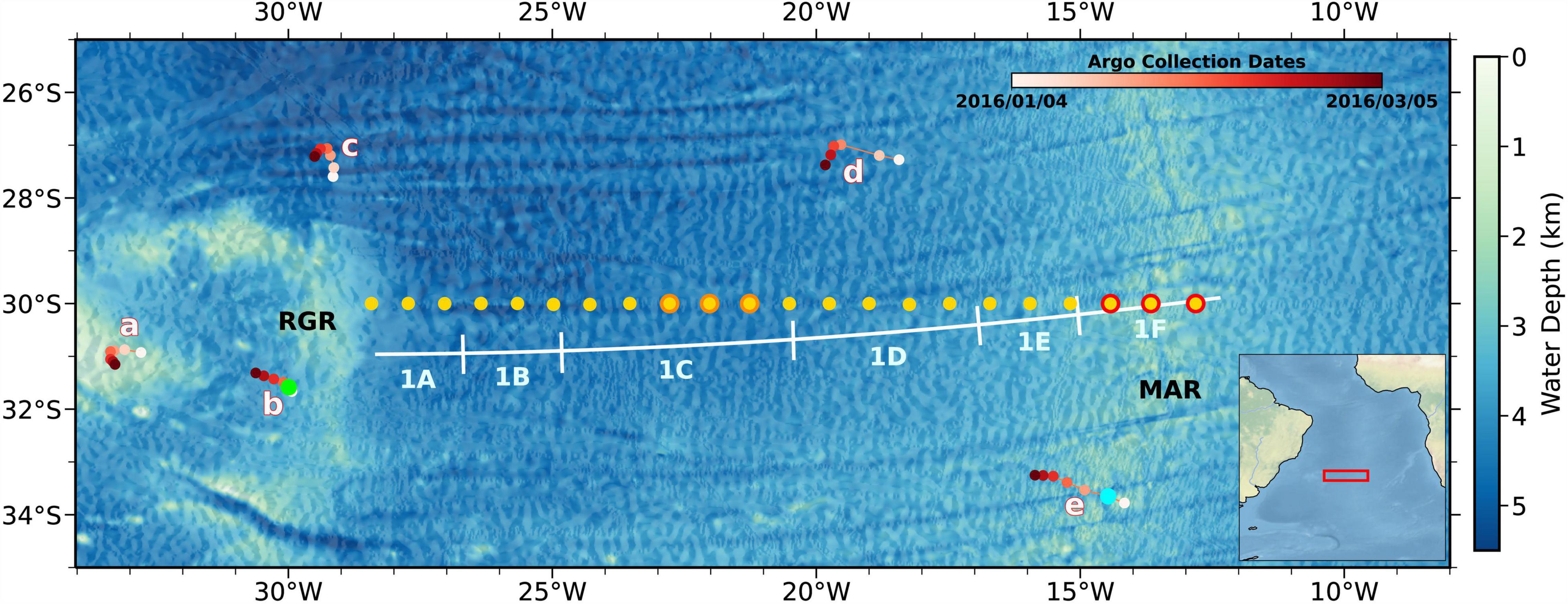
Figure 1. Bathymetric map of seismic survey location. Bathymetry from the Global Multi-Resolution Topography Synthesis (Ryan et al., 2009). White lines = seismic profiles collected between January 29 and February 14, 2016, short meridional lines mark the connection point between zonal lines; yellow dots = CTD casts from GO-SHIP survey acquired in October 2011, yellow dots with orange/red edges correspond to orange/red profiles in Figure 2 (GO-SHIP 2003 CTDs within 0.5° of 2011 CTDs and are not shown); red dots = Argo float trajectories between January 4 and March 5, 2016, labeled a–e; green and cyan dots = Argo floats used for mixing calculation to compare with seismic results in Figure 6. RGR, Rio-Grande Rise; MAR, Mid-Atlantic Ridge. Inset shows regional setting, with red box marking the location of the study area.
More recently, studies have shown that storms are an effective method of wind energy injection (Dohan and Davis, 2011). In the wake of storms, diapycnal diffusivity is enhanced by 9 × 10⁻⁵ m2 s–1 (Jing et al., 2015). Quantifying the effect of storms on oceanic mixing is especially difficult as they are moving, short-duration events. Conventional one-dimensional (1D) hydrographic measurements such as CTDs and Vertical Microstructure Profilers (VMPs) are unlikely to capture their effects. In particular, little is known about how storms contribute to mixing in the quiescent ocean interior, especially in basins like the central South Atlantic that are not covered by storm tracking system such as NOAA. In a warming world with increasing storm intensity (Walsh et al., 2019), it is important to develop two-dimensional (2D) tools that can yield a deeper understanding of the effects of storms on ocean mixing.
Seismic oceanography (SO) is a powerful tool that can be used to overcome these observational gaps. SO provides observations of physical processes across a horizontal length scale of ∼O(105) m to ∼O(102) m (Ruddick, 2018). The method utilizes low frequency (e.g., 5–120 Hz) acoustic sources and towed cable(s) containing a dense array of hydrophones to receive acoustic energy that is transmitted and reflected at boundaries created by temperature and salinity differences. Nandi et al. (2004) demonstrated that SO is able to capture temperature difference as small as 0.03°C. Sallarès et al. (2009) further confirmed that reflectivity has a stronger correlation with temperature than salinity. The frequency bandwidth of the acoustic source is capable of imaging thermohaline fine structure with lateral and vertical resolutions on the order of 10 m, meaning that the method is capable of mapping mesoscale structures such as fronts, internal waves, and eddies that are always missing in conventional hydrographic measurements. This relatively high resolution makes SO an ideal method for turbulence mixing analysis. Studies that calculated turbulent diffusivities from slope spectra of seismic reflections demonstrate the suitability of the method in exploring spatial and temporal changes of mixing (Sheen et al., 2009; Fortin et al., 2016; Mojica et al., 2018; Tang et al., 2019; Dickinson et al., 2020). The instantaneous spatial distribution of mixing derived from seismic data represents a near-full energy cascade from internal waves to turbulence (Ruddick, 2018), implying the potential use of seismic derived parameterization in future ocean models (Tang et al., 2021). When combined with hydrographic data, seismic oceanography studies can be used to overcome significant observational gaps.
Here, we present and analyze a ∼1,600 km-long 2D seismic transect starting from the eastern edge of the Rio Grande Rise (RGR) to the MAR, covering one of the major pathways of the Atlantic meridional overturning circulation (Figure 1). We calculate diapycnal diffusivities across the thermocline using the slope spectra method with seismic sections, as well as using finescale parameterization with CTD and Argo data. Our primary objective is to examine the spatial distribution of mixing in the central South Atlantic thermocline and extend its observational record. We also present the most likely hypotheses for drivers of enhanced mixing. Our results extend the observational record of diapycnal mixing in the central South Atlantic thermocline by providing diffusivities in 2003, 2011, and 2016, and provide further insights into the drivers of mesoscale mixing variability.
Data and Methods
Seismic Data and Processing
This research uses seismic reflection data collected during the Crustal Reflectivity Experiment Southern Transect (CREST) experiment aboard the R/V Marcus G. Langseth (Estep et al., 2019). The primary goal of the CREST survey was to investigate the evolution of oceanic crust at 30° S, and it spans the eastern edge of the RGR to the MAR, including a ∼1,600 km-long continuous east-west data transect (Figure 1). The transect sits at the center of the South Atlantic subtropical gyre and provides an opportunity to investigate the change of mesoscale mixing processes along a significant distance in a region that contains the returning limb of the Atlantic meridional overturning circulation (Cabré et al., 2019).
Seismic data were collected between January and February of 2016 (Figure 4). The acoustic source was a 36 bolt air-gun array with a total volume of 6,600 in3 and 37.5 m shot spacing. Acoustic records were collected using a 12.6 km acoustically sensitive cable (i.e., streamer). The streamer contained 1,008 hydrophones with 12.5 m spacing. This survey design collects repeat reflections from the same subsurface point (i.e., common mid-points, CMPs) every 6.25 m. To ensure the maximum depth of imaging to be more than 1,000 m, while maintaining a high signal-to-noise ratio for turbulence analysis, we used the first 400 near-source acoustic records.
Seismic data were processed with a standard, but adapted, processing sequence typically used to image the solid earth (Yilmaz, 2001): geometry definition, noise attenuation, CMP sorting, sound speed analysis, stacking, amplitude correction, and migration (Fortin and Holbrook, 2009; Hobbs et al., 2009). Particular adaptations were made in the noise attenuation step to produce a high-quality image of oceanic fine structures. First, an eigenvector filter is applied to remove the direct waves that overprint the first 1 s of data. Second, the relatively small shot spacing (37.5 m) generates reverberations between the sea surface and seafloor which share the same frequency range with primary signals. We filter out reverberations in the frequency-wavenumber domain based on the curvature differences between these coherent noises and primary signals in shot gathers. Thirdly, to reliably extract turbulent regimes from seismic data, random noise must be attenuated, we follow the recommendations of Holbrook et al. (2013) by applying a 30–80 Hz band-pass filter. Lastly, shot-generated harmonic noise is suppressed by applying a notch filter centered at harmonic spikes (every 0.0267 cpm, cpm = cycles per meter) in the wavenumber domain (Holbrook et al., 2013). In addition, we implement a denoising convolutional neural network (DnCNN) to suppress random noise after stacking. We use the recommended steps and parameters of 17 layers and a mini-batch size of 128 (Zhang et al., 2017; Jun et al., 2020). We train the DnCNN model for 40 epochs and the number of iterations within each epoch is 220. After a series of noise attenuation, the signal-to-noise ratio of the entire seismic data increases by a factor of 6.
Seismic-Derived Diffusivities
Background
Based on the assumption that seismic reflections are a reasonable approximation of isopycnal surfaces (Krahmann et al., 2009; Holbrook et al., 2013), studies have shown that turbulent diffusivity can be accurately measured from vertical displacement spectra of tracked reflections (e.g., Figure 3A) from both the internal wave subrange (Sheen et al., 2009; Dickinson et al., 2017) and turbulent subrange (Holbrook et al., 2013; Fortin et al., 2016; Mojica et al., 2018; Tang et al., 2019; Gunn et al., 2021). To clearly recognize the transition from internal wave regimes to turbulent regimes in log-log space, the vertical displacement spectra are multiplied by (2πkx)2 to produce the slope spectra. Here we estimate the turbulent dissipation rate ε through the slope spectra method in the turbulent subrange, , via a model proposed by Klymak and Moum (2007):
where Γ = 0.2 is the empirical mixing efficiency (Osborn and Cox, 1972), N is the horizontally averaged buoyancy frequency calculated from 22 historical CTD casts within the survey area (Figure 2C, black line), CT = 0.4 is the Kolmogorov constant, and kx is the horizontal wavenumber. Equation (1) produces a turbulence subrange with a slope of +1/3 in log-log space. Diapycnal diffusivity, K, is then calculated using the Osborn relationship (Osborn, 1980):
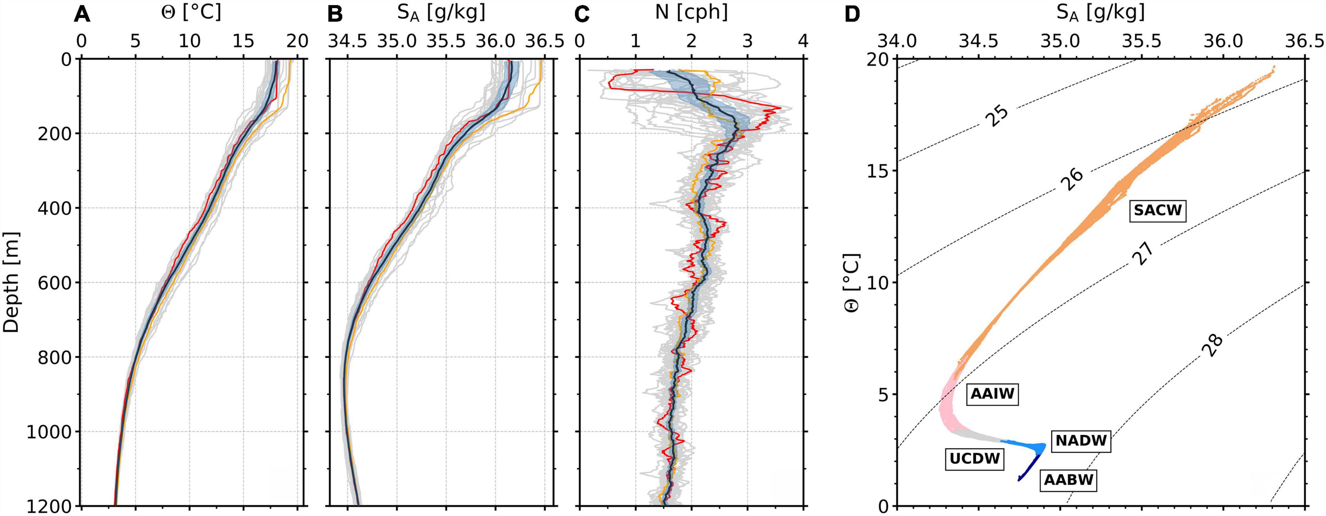
Figure 2. Water properties from 22 GO-SHIP 2011 CTD casts (yellow dots in Figure 1). (A) Conservative temperature, Θ, as a function of depth. Black line = average profile; gray lines = individual profiles; blue patch = 95% confidence interval; and red/orange lines = average profiles of CTDs with red/orange edges (Figure 1). (B) Absolute salinity, SA, as a function of depth. (C) Buoyancy frequency, N, as a function of depth. [cph = cycles per hour]. (D) Conservative temperature (Θ) – Absolute salinity (SA) diagram. Points colored according to the water mass definition of Hernández-Guerra et al. (2019). Orange dots = South Atlantic Central Water (SACW); pink dots = Antarctic Intermediate water (AAIW); gray dots = Upper Circumpolar Deep Water (UCDW); blue dots = North Atlantic Deep Water (NADW); dark blue dots = Antarctic Bottom Water (AABW). Labeled dotted lines = potential density anomaly surfaces.
where ε is spectrally estimated from seismic data and varies as a function of distance along the section and depth.
To generate high-resolution maps of diffusivity across the entire seismic section, two complementary methods are used to calculate K. These methods allow us to extract turbulent information across a range of depths and scales, as they take advantage of both low and high amplitude reflectivity (Fortin et al., 2016).
Relative Turbulent Energy From Amplitude Spectra
First, amplitude spectra are calculated following Holbrook et al. (2013) through direct Fourier data transform. These spectra are calculated directly from seismic amplitudes (i.e., no tracking) along depth slices, and are first used to identify whether the turbulent subrange exists. For the CREST data, the turbulent subrange exists between kx 0.025–0.045 cpm (22.2–40 m) (Figure 3B). The advantage of using amplitude spectra is reflected in its preservation of all horizontal wavenumbers, therefore relative turbulent energy from all reflections can be extracted. In other words, amplitude spectra can provide relative levels of turbulence across the entire seismic section. However, amplitude spectra cannot provide absolute diffusivities because they are affected by the variation of seismic amplitudes, it is necessary to scale them with absolute diffusivities calculated from slope spectra of tracked reflections (hereafter, reflector slope spectra).
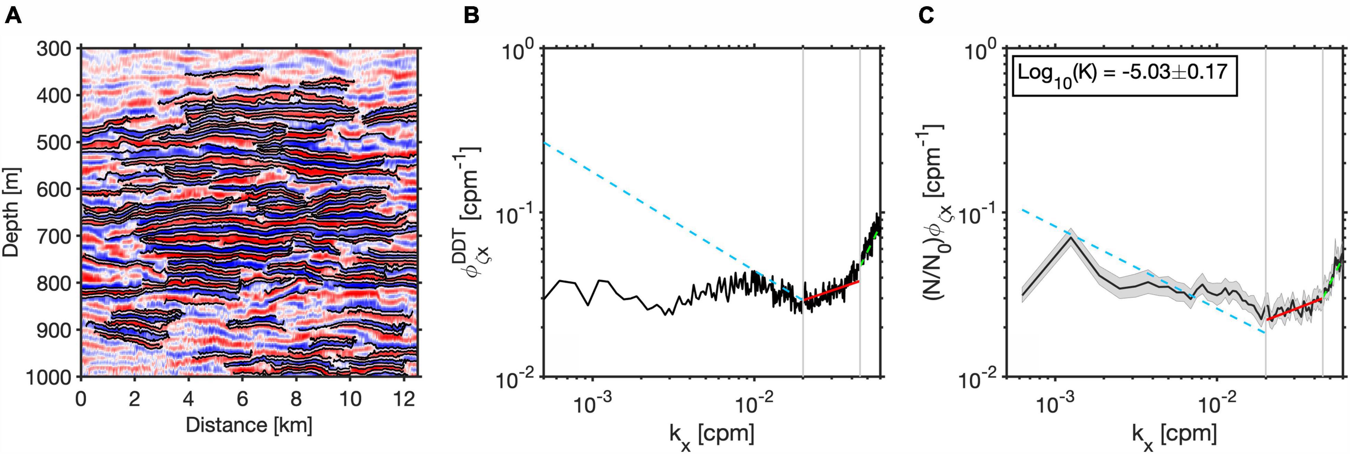
Figure 3. Example of spectral analysis from line 1A (a rolling window used in section “Zonal Variability of Diffusivities”). (A) Seismic data overlapped with tracked reflections. Black lines = tracked reflections. (B) Direct data transform (DDT) of seismic data in panel (A). (C) Average slope spectrum calculated from all the tracked reflections in panel (A). Shaded gray area = 95% bootstrap confidence intervals. Dashed blue lines (k– 1/2), solid red lines (k1/3) and dashed green lines (k2) = the internal wave subrange, turbulence subrange and white noise, respectively (Garrett and Munk, 1975; Klymak and Moum, 2007; Holbrook et al., 2013). Two vertical gray lines bound the turbulent subrange used to calculate diffusivity. The calculated diffusivity and its uncertainty are shown in the upper left corner.
Absolute Diffusivities From Reflector Slope Spectra
Reflector slope spectra are calculated based on vertical displacement of undulating reflections that follows isopycnals, they are independent of seismic amplitude and thus can be used to estimate absolute diffusivity. We calculate reflector slope spectra using Fourier transform lengths of 256 points as recommended by Holbrook et al. (2013), equivalent to a reflection length of 1.6 km. Turbulent dissipation is then estimated by fitting reflector slope spectra to model (1) within the previously identified turbulent subrange (0.025–0.045 cpm) using least square inversion. Diffusivity is then calculated using equation (2) (Figure 3C).
Using reflector slope spectra also has its limitations. Tracked reflections, that yield slope spectra, must have high amplitude and good continuity, corresponding to the steepest temperature and salinity gradients (Ruddick et al., 2009). This limitation implies that absolute diffusivities cannot be estimated from weaker and discontinuous reflections that still possess turbulent information. Lower reflection amplitudes represent lower temperature and salinity gradients, corresponding to weaker stratification regions that are prone to mixing. Discontinuous reflections could be caused by mixing instabilities such as interleaving, internal wave breaking, turbulence, and double diffusion (Tang et al., 2018). Therefore, a simple spatial smoothing of diffusivities calculated from stronger and continuous reflections over the entire seismic section could result in underestimation of diffusivities in areas of weaker and discontinuous reflections. As discussed above, because amplitude spectra preserve all horizontal wavenumbers regardless of the strength of the reflections, we can overcome this limitation by joining and applying these two techniques in different window sizes to honor turbulent information in both types of reflections.
Combining Amplitude and Reflector Slope Spectra
The seismic section is divided into regional windows of size 6.25 km wide and 50 m deep for reflector slope spectra analysis. The size of the window is chosen to include enough reflections to minimize artifacts and provide accurate estimations of absolute diffusivities. An average reflector slope spectrum is calculated from all the tracked reflections within each regional window, and an absolute diffusivity is estimated for that window (Figure 3C). To complement the reflector slope spectra method, we calculate amplitude spectra in a much smaller window size of 400 m wide and 10 m deep. The window width is determined to include at least 10 horizontal wavelengths as calculated from the lower bound of the identified turbulent subrange (Fortin et al., 2017). Then, by integrating amplitude spectra energy over the turbulent subrange within each window, a map of relative turbulent energy across the entire seismic section can be obtained. Finally, relative turbulent energy is scaled by the absolute diffusivities within each regional window to produce the final high-resolution diffusivity map which has a horizontal and vertical resolution of 400 and 10 m, respectively (Figure 5). Fortin et al. (2016, 2017) have shown that this technique can reliably measure turbulent diffusivities from weaker reflections and seismically transparent zones where mixed water resides. Thus, these complementary techniques are able to produce high-resolution 2D maps of diffusivities. To avoid inaccurate estimation of diffusivity, seismic data shallower than 200 m are discarded because of the contamination caused by residual direct wave energy.
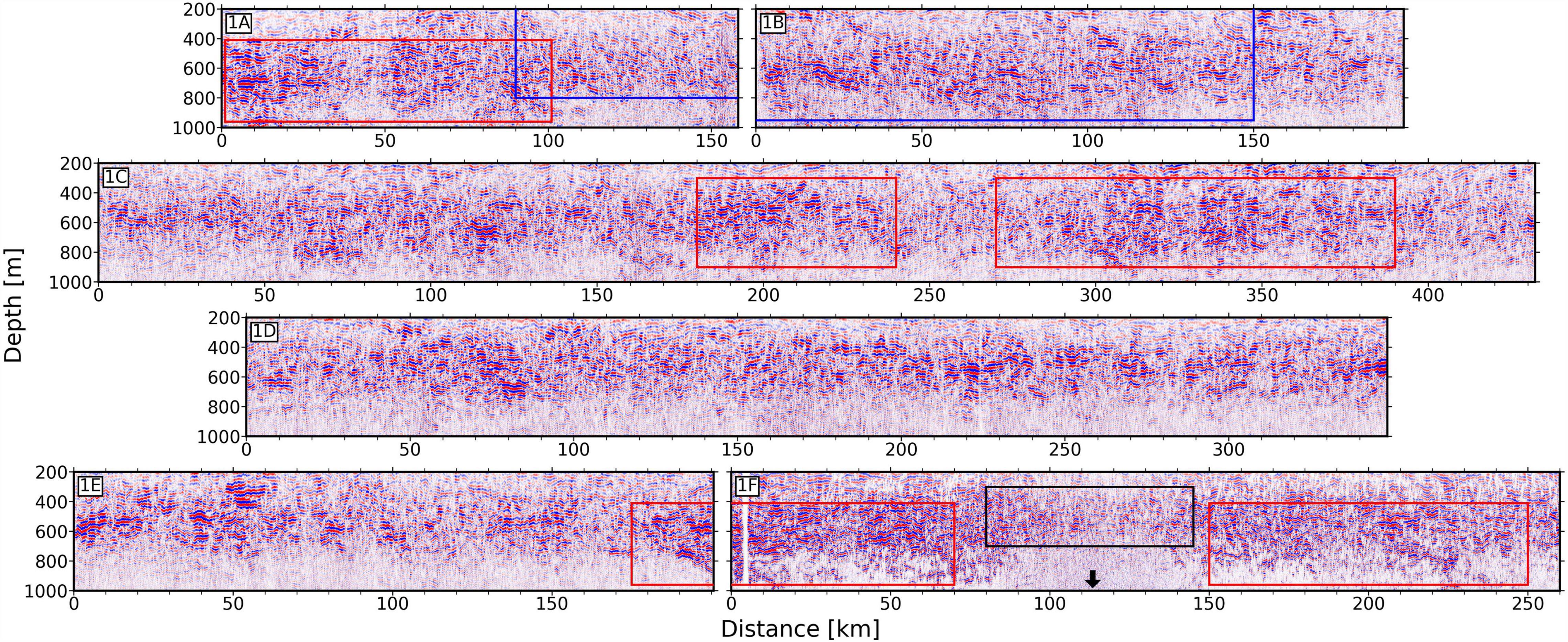
Figure 4. Seismic sections from west (line 1A) to east (line 1F). Red boxes = locations of continuous, high amplitude reflections; blue boxes = an example location of shorter, discontinuous reflections; black box = water mass above the MAR. Black arrow = location of crest of the MAR.
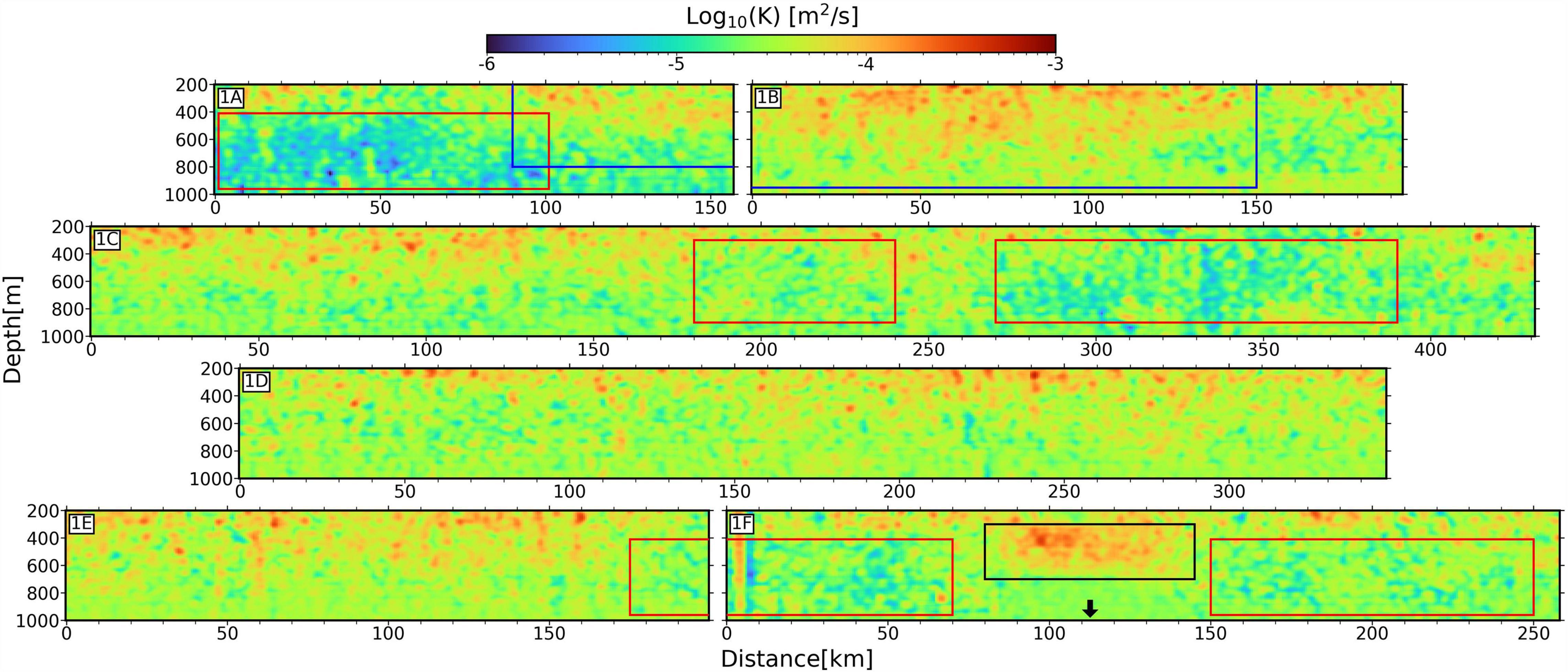
Figure 5. Turbulent diffusivity maps derived from seismic sections in Figure 4. Red boxes = locations of lower diffusivities; blue boxes = an example location of enhanced mixing; black box = enhanced mixing above the MAR. Black arrow points at the location of the crest of the MAR. Colored boxes are the same as in Figure 4.
Depth- and Zonally-Averaged Diffusivity
We investigate the distribution of thermocline diffusivities as functions of longitude and depth by taking appropriate means (Figure 6). So that seismic-derived diffusivities are comparable with lower resolution hydrographic data, we calculate depth-averaged, zonally varying diffusivities in rolling half overlapping windows. The window starts at the beginning of line 1A to the end of line 1F, covering a total length of 1,625 km and has a width of 12.5 km, with an overlap of 6.25 km. The depth range of each window is 300–1,000 m, for which the starting depth is chosen to match Argos and CTDs depth limitations. Within each window, depth-averaged diffusivity is estimated using the average reflector slope spectrum (e.g., Figure 3C), rather than the amplitude spectra. The average diffusivity within each window is assigned to the center longitude of that window. Ultimately, we obtain depth-averaged diffusivities that span longitudes 28.3° W to 12.4° W with a sampling interval of 6.25 km (Figure 6).
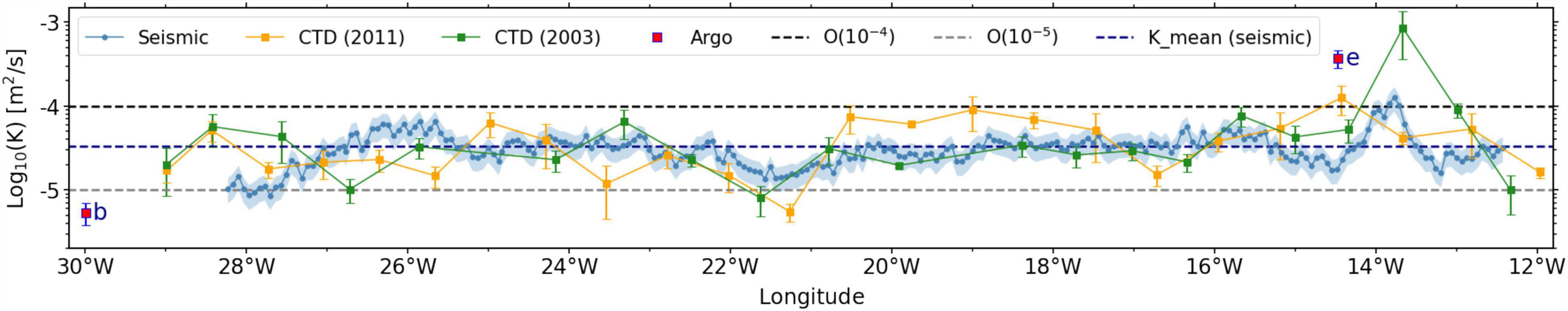
Figure 6. Depth-averaged diffusivities derived from seismic and CTDs in the zonal direction, plotted with depth-averaged diffusivities calculated from two Argo profiles (green and cyan dots in Figure 1). Blue shade represents uncertainties of seismic estimates discussed in section “Depth- and Zonally-Averaged Diffusivity.” Error bars show the standard error of depth-averaged diffusivity of CTD/Argo profiles.
Zonal-averaged, depth-varying diffusivities are calculated based on their topographic setting. Each seismic section is divided vertically into 256 m half-overlapping windows and into regions above smooth and rough topography. Within each window, an average spectrum is calculated to estimate diffusivity. Diffusivities derived from different seismic sections are normalized by the lengths of the sections then horizontally averaged to produce zonal-averaged, depth-varying diffusivities.
Error Analysis
Following Dickinson et al. (2020), we conservatively estimate an uncertainty for seismically derived diffusivities as ±0.4 logarithmic units. This value combines sampling and methodological errors. The sampling error mostly derives from the uncertainty in N, which we estimate as 0.28 cph using the standard deviation of CTD data. Methodological errors include the assumption of constant CT and Γ and the process of fitting a straight-line model to reflector slope spectra. These uncertainties have been quantified by Dickinson et al. (2020), and are 0.25 log units. Combined in quadrature, the total uncertainty is ± 0.4 logarithmic units.
Conductivity-Temperature-Depth- and Argo-Derived Diffusivities
Diffusivities are estimated from CTD and Argo data and can be seen as representative of mean and spot measurements of mixing, respectively. We estimate diffusivities from five nearby Argos and 44 co-located CTDs (Figure 1). We use CTD datasets from two repeat surveys occupying GO-SHIP A10 transect in 2003 and 2011 at 30° S (Sloyan et al., 2019). Argos were collected around the same time as the seismic survey (data downloaded from Global Argo Data Repository). All of the Argo profiles used in this study record depths larger than 1,000 m, and have vertical resolution less than 10 m. Argos b and e are ideally placed to provide spot measurements of mixing above smooth and rough topography conditions, respectively. Argo b was collected 176 km from the western end of line 1A, above the RGR, and only 2 days before the start of seismic acquisition (Figure 1, green dot). Argo e traveled across the MAR during January 2016 and is used to compare with seismically derived and depth-averaged diffusivities across the MAR (Figure 1, cyan dot). Although the Argo data are not co-located with the seismic survey, they provide meaningful measurements of the oceanic field above similar geological settings at two key locations.
From these hydrographic profiles, we computed potential density and buoyancy frequency. The selected profiles were then divided into 256 m half-overlapping segments. Following Kunze et al. (2006), the shallowest segment (0–256 m) is discarded due to the presence of sharp pycnoclines. For the remaining segments, we use a strain-based finescale parameterization to estimate ε (Kunze et al., 2006):
ε0 = 6.73 × 10⁻¹⁰ m2 s–2, N0 = 5.24 × 10⁻³ rad s–1, is the observed strain variance, is the strain variance from the Garrett-Munk model spectrum (Garrett and Munk, 1975). is the vertically averaged buoyancy frequency for each segment, which is estimated as linear fits to the specific volume anomaly depth profiles using the adiabatic leveling method (Bray and Fofonoff, 1981). H(Rω) is a function related to the shear-to-strain ratio Rω, which is set to 7 in this study (Kunze et al., 2006). L(f,N) is a correction for the effects of latitude (Gregg et al., 2003). Finally, the diffusivity is given by equation (2).
Results
Thermocline Structure
The thermocline is visible as a 1,000 m thick band of reflectivity that extends 1,600 km across all seismic sections and is consistent with the regional temperature structure (Figures 2A, 4). Between 0 and 800–900 m depth, we observe stronger reflections and weaker reflectivity at greater depths. This vertical distribution of reflection amplitude corresponds to highly stratified SACW and weakly stratified AAIW, respectively (Figure 2). At 800–900 m depth, weakening reflection amplitude shows zonal variability indicating that the depth of the SACW/AAIW boundary shoals eastward by 100 m (Figure 4,1A).
Within the thermocline, reflectivity varies greatly in the lateral direction, changing from longer, higher amplitude to, shorter, lower amplitude and more disrupted reflectivity. Mesoscale patches of high-amplitude and more continuous reflectivity suggest the presence of eddy-scale processes, these patches extend to depths of 900 m and across tens of kilometers zonally (Figure 4, red boxes). Between 90 km and 150 km (Figure 4, blue boxes), a set of shorter, discontinuous reflections dip to the east which we interpret as a shear event typical of the region. We do not observe submesoscale structures here, although these are often found in more energetic ocean environments such as boundary currents.
Above the MAR, reflections are clearly disrupted. In line 1F from 80 to 150 km weaker discontinuous reflections can only be seen from the surface down to 700 m (Figure 4, black box and arrow). This anomalous patch of low reflectivity extends approximately 30 km on either side of the ridge. Data below 700 m are severely contaminated by noise that has been diffracted by the hard igneous seafloor of this mid-ocean ridge and is too complicated to be sufficiently removed using noise attenuation.
Diffusivity of the Central South Atlantic Thermocline
Across the 1,600 km section of the central South Atlantic thermocline, the mean seismic-derived diffusivity is 3.96 × 10⁻⁵ m2 s–1 (Figure 5). The value is similar to the microstructure observations made almost 20 years earlier in the Brazil Basin at longitudes of 28° W to 16° W (Polzin et al., 1997). The authors found a mean diffusivity of 1–5 × 10⁻⁵ m2 s–1 in the upper 1,000 m of the water column. These seismic-derived (2016) and microstructure (1996) values are also consistent with CTD-derived diffusivities, which can be seen as representative of means for 2003 and 2011. The mean CTD estimates for 2003 and 2011 are 7.45 × 10⁻⁵ m2 s–1 and 4.15 × 10⁻⁵ m2 s–1, respectively. The 2003 estimate is biased high by an anomalously elevated diffusivity around 13.5° W (Figure 6, green line). When this point is removed, the mean decreases to 3.57 × 10⁻⁵ m2 s–1 which is remarkably consistent with the 2011 measurement and the mean seismic-derived diffusivity.
The spatial standard deviation of the seismic estimates is of a similar magnitude, 2.9 × 10⁻⁵ m2 s–1, to the mean revealing the heterogeneity of the thermocline diffusivities. Variability is clearly related to variations in the thermocline structure, as we observe a strong correlation between seismic reflection amplitudes (i.e., strength of stratification) and corresponding diffusivity maps. Weaker and discontinuous reflections are found to have an average diffusivity of 4.79 × 10⁻⁵ m2 s–1, a factor of four greater than locations dominated by stronger and more continuous reflections that have a mean value of 1.2 × 10⁻⁵ m2 s–1. This spatial correlation is most apparent in lines 1A,B. From the beginning of line 1A to about 90 km [Figure 4,1A (red box)], where seismic reflections appear to be stronger and laterally continuous, the corresponding diffusivity map shows low diffusivities close to the canonical value of 1 × 10⁻⁵ m2 s–1 [Figure 5,1A (red box)]. However, starting at 100 km and moving eastward into line 1B, the strength of seismic reflections diminish as they become discontinuous [Figures 4,1A,B (blue boxes)], while diffusivities start to increase to the level of 10 × 10–5 m2 s–1 from shallower water (∼250 m) into deeper water (∼900 m). In line 1B, at about 120 km, diffusivities start to gradually increase from deeper water (∼800 m) to shallower water (∼300 m), and eventually form a bowl-shape region populated by diffusivity hotspots across lines 1A,B [Figures 5,1A,B (blue boxes)]. Similar correlation patterns between the seismic images and diffusivity maps can also be observed in all remaining profiles.
Taken as a whole, there are identifiable mesoscale patterns in the diffusivity. In areas that show elevated diffusivities, diffusivity hotspots of 7.5–10 × 10–5 m2 s–1 largely dominate, while scattered higher diffusivities of 20–50 × 10–5 m2 s–1 also exist. These hotspots are mostly located in the upper 600 m, with an exception in line 1B from 50 to 100 km where they spread deeper than 800 m. In lower diffusivity regions, we see the canonical background value of 1 × 10⁻⁵ m2 s–1 that mostly resides in the mid-depth from 400 to 800 m; diffusivities are slightly higher outside of this depth range.
Above the MAR, we observe the highest diffusivities of 25–50 × 10–5 m2 s–1 that are densely distributed from 80 to 150 km within the 300 to 700 m depth range (Figure 5,1F). These estimates show that diffusivities are enhanced by an order of magnitude compared with background values. No reflections were tracked below 700 m because of severe noise contamination, which hinders our ability to reliably calculate diffusivities at deeper depths (Figures 4, 5,1F). Nevertheless, the signal-to-noise ratio for the 300–700 m depth range is high enough for diffusivity estimation. Away from the ridge crest, diffusivities rapidly decay to about 1 × 10⁻⁵ m2 s–1 within ∼30 km.
Zonal Variability of Diffusivities
Depth-averaged diffusivities reveal zonal variability in thermocline diffusivity, which is heterogenous of mesoscale length scales. Depth-averaged diffusivities vary from 0.9 × 10⁻⁵ to 12.6 × 10⁻⁵ m2 s–1, with the highest diffusivity above the MAR. Around 26° W, there is a second region of elevated diffusivity of 6.5 × 10⁻⁵ m2 s–1. Diffusivities are lowest in the west at approximately 1 × 10⁻⁵ m2 s–1. These depth-averaged diffusivities serve as an instantaneous snapshot of mixing during February 2016. They reveal that there is no zonal trend in diffusivities, rather diffusivities are enhanced in localized patches.
We now compare seismic-derived diffusivities to hydrographic-derived and depth-averaged diffusivities. CTD-derived and depth-averaged (mean taken over 300–1,000 m) diffusivities that vary with longitude range between 0.6 × 10⁻⁵ m2 s–1 and 85 × 10–5 m2 s–1 (GO-SHIP 2003, 2011; Figure 6, green and yellow line). The CTD estimates increase by one order of magnitude at the MAR. Two Argo profiles above smooth and rough topographic conditions serve as spot measurements of turbulence tuned to differing bathymetric conditions (Figure 6, magenta squares). The diffusivity calculated from Argo b (smooth) is 0.5 × 10⁻⁵ m2 s–1, it has a similar magnitude to the western end of line 1A, which has a seismic-derived diffusivity of 0.9 × 10⁻⁵ m2 s–1. Diffusivities above the rough topography of the MAR calculated from Argo e (37 × 10–5 m2 s–1) and seismic (12 × 10–5 m2 s–1) are both one order of magnitude higher than over smooth topography and are within error of each other (Figure 6).
Depth Variability of Diffusivities Over Different Topographic Settings
Zonally averaged diffusivities reveal the depth response of thermocline diffusivities over smooth (Figures 7A–C) and rough (Figures 7D–F) topographic settings. Above smooth topography, diffusivities are fairly constant with depth and are typically 1 × 10⁻⁵ m2 s–1. There is little difference between the seismic- and CTD-derived diffusivities here. Above rough topography, diffusivities are enhanced everywhere in the upper 700 m, and are 5.5 × 10⁻⁵ m2 s–1 for seismic-derived estimates and 2.7 × 10⁻⁵ m2 s–1 to 17 × 10–5 m2 s–1 for CTD-derived estimates (Figures 7D,E). Below 700 m, seismic data cannot reliably recover diffusivities because of noise contamination, and the CTD data are used to fill this gap. The deep CTD-derived estimates show a sharp increase from 600 to 1,000 m (Figure 7D). We find that, at 30° S in the South Atlantic Ocean, diffusivities across the entire thermocline (up to 1,000 m depth) are modified by the presence, or lack of, rough topography (e.g., compare Figures 7C,F).
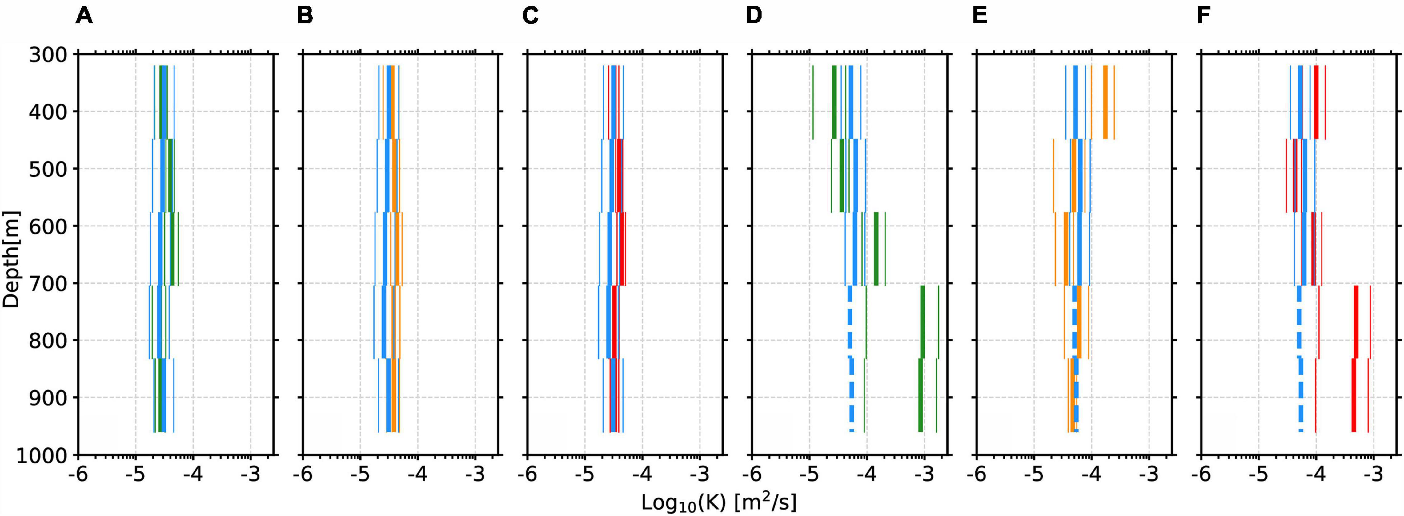
Figure 7. (A–C) Averaged vertical profiles of diffusivity above smooth topography (data from seismic lines 1A–E and CTDs west of 15° W). Thick blue bars, green bars, orange bars = averaged vertical profiles derived from seismic, GO-SHIP CTD 2003, and 2011, respectively. Red bars = averaged vertical profiles derived from both GO-SHIP 2003 and 2011. Thin bars represent standard errors between CTD profiles or seismic sections. (D–F) Same to (A–C) but above the MAR (data from seismic line 1F and the three eastern most CTDs from GO-SHIP 2003 and 2011). Dashed blue lines represent unreliable diffusivities calculated from regions contaminated by noise.
Discussion
Here, we extend the observational record of ocean interior diapycnal mixing in the central South Atlantic, and, for the first time, we resolve diffusivities at mesoscale lengths for this location. High-resolution seismic diffusivity maps provide an unprecedented view of the variability of diapycnal mixing across 1,600 km of the thermocline. By combining high-resolution seismic-derived diffusivities with low spatial resolution CTD-derived and low temporal resolution Argo-derived diffusivities, we can assess the likely drivers of mixing in this location.
Temporal and Spatial Variability of South Atlantic Thermocline Diffusivities
At synoptic (∼1,000 km) and decadal scales, the background diffusivity of the South Atlantic thermocline has changed little at this location. In 1996, direct turbulent diffusivities measurements across the Brazil Basin revealed that the upper 1,000 m of the South Atlantic typically had diffusivities of around 1–5 × 10⁻⁵ m2s–1 (Polzin et al., 1997). CTD-derived mixing estimates from 2003 and 2011 also show a mean diffusivity of 3–4 × 10⁻⁵ m2 s–1, while seismic data collected in 2016 show a similar mean diffusivity in the upper 1,000 m of 4 × 10⁻⁵ m2 s–1. Taken together, these four decadal snapshots (1996, 2003, 2011, and 2016) suggest that there is little variability in the mean diffusivity of the thermocline. Using a global coupled climate model, Hieronymus et al. (2019) found that oceanic background diffusivity has a significant impact on the climate. They found that increased background diffusivity leads to increased meridional heat transport and stronger overturning in the ocean. Our observations suggest that on decadal time-scales the mean thermocline diffusivity has changed little in this location, which may imply steady meridional overturning circulation in the South Atlantic thermocline.
Imprinted upon the background diffusivity, we show that diffusivities are heterogeneous and can be enhanced by up to one order of magnitude. Regions of high mixing correspond to seismic transparent zones or disrupted reflections. The correlation between seismic reflectivity and turbulent mixing is typical of seismic oceanography studies (Dickinson et al., 2017; Fortin et al., 2017; Tang et al., 2021) and these observations have shown that higher reflectivity is caused by sharper temperature and salinity gradients, hence stronger stratification, while lower reflectivity represents weaker stratification that facilitates mixing or homogeneous water masses. Weakened reflectivity above the MAR corresponds to enhanced mixing and weaker stratification (Figure 4, black box). Seismic-derived, CTD-derived, and Argo-derived diffusivities are all enhanced by an order of magnitude. This result is consistent with lower resolution diffusivity measurements made by Polzin et al. (1997), who showed that diffusivities exceed 1 × 10⁻⁵ m2s–1 in the thermocline above the ridge. Depth-averaged N shows stronger stratification (2.13 cph) above smooth plains compared to weaker stratification (2.01 cph) above the MAR (Figure 2C). The high resolution and depth coverage of the seismic data also reveal that mixing across the entire thermocline (200–1,000 m) is enhanced within 30 km of the ridge. Away from the ridge, several other patches of high-diffusivity are observed that also correspond with low amplitude and disrupted reflectivity.
The spatial heterogeneity of mixing suggests that the mid-ocean thermocline is not quiescent. Enhanced mixing in the ocean interior is primarily caused by breaking of internal waves (Gregg et al., 2003) for which the energy input generally comes from tidal flows impinging upon topography (Munk and Wunsch, 1998) and wind forced near-inertial waves below the mixed layer (D’Asaro, 1985; Alford, 2003b). We discuss the possible drivers of observed enhanced mixing below.
Drivers of Enhanced South Atlantic Thermocline Diffusivities
Rough Topography at the Mid-Atlantic Ridge
Enhanced mixing in the thermocline above the MAR is most likely driven by barotropic tides impinging on the rough bathymetry of the ridge. Due to a lack of observations, the effect of the MAR on upper water column (<1,000 m) mixing has been less clear than its effect on abyssal water. Here, both seismic-derived and hydrographic-derived estimates of K show that diffusivities across the entire water column are enhanced by at least one order of magnitude compared with background values. These rates are consistent with shallow microstructure observations above mid-ocean ridges (Polzin et al., 1997; Mauritzen et al., 2002; St Laurent and Thurnherr, 2007) and recent work by Li and Xu (2014) who found the influence of rough topography on turbulent mixing can extend 3,300 m upward into the ocean interior. Seismic estimates (limited to 700 m) show larger diffusivities at shallow depths (Figure 5,1F), while microstructure measurements show that diffusivities increase significantly below 700 m depth, as found by Polzin et al. (1997). Therefore, it is also possible that an upward source or mesoscale oceanic process is enhancing the shallow mixing further and is only captured by the high-resolution siemsic data. Due to the presence of the ridge and consistency of these high diffusivities over time, we conclude that at 30° S, the MAR enhances diffusivities across the entire water column by at least one order of magnitude.
The rapid decay of diffusivities within ∼30 km away from the MAR is shorter than similar decays of ∼60 km at the Hawaiian Ridge and the Mariana Ridge (Klymak et al., 2006; Tang et al., 2021). This discrepancy indicates that at the Hawaiian Ridge and the Mariana Ridge, a large portion of tidal energy radiates away, while at the MAR, a significant portion of tidal energy is dissipated locally, which is consistent with previous interpretations (Waterhouse et al., 2014).
Storm and Eddy
The causes of enhanced mixing over smooth topography are less clear. Irregular patches of enhanced mixing in these seismic lines could be caused by a variety of mechanisms, such as dissipation of high-mode near-inertial energy, breaking of low-mode tidal or near-inertial waves through wave-wave interactions, and energy dissipation through mesoscale eddy fields (MacKinnon et al., 2013). Numerical studies predict enhanced mixing caused by dissipation of semidiurnal tides near latitudes of 29° N/S (MacKinnon and Winters, 2005; Simmons, 2008).
Of these mechanisms, wind-induced mixing is the most pervasive globally (Alford et al., 2016). Winds inject energy into the ocean through wind stress impulses such as traveling midlatitude storms. These storms can excite frequency response in the near-inertial band and generate near-inertial internal waves (Pollard, 1970; Gill, 1984; Alford et al., 2016). Horizontal convergence and divergence of the ocean’s mixed layer can provide pathways for wind injected energy to propagate downward and eventually generate near-inertial waves in the stratified water below (D’Asaro, 1985; D’Asaro et al., 1995; Young and Jelloul, 1997). Much of the energy exerted by winds goes into low-mode near-inertial waves that propagate for great distances (D’Asaro et al., 1995; Alford, 2003b), while the remaining portion oscillates as high-mode near-inertial waves that promote mixing because of their potential for higher shear (Alford and Gregg, 2001; Alford, 2010). Thus, in our study, enhanced mixing over smooth topography may reveal the energy cascading process of high-mode near-inertial waves breaking into small-scale turbulence during downward propagation. In addition, using Lagrangian observations, Chaigneau et al. (2008) showed that winds inject near-inertial energy into the mixed layer in the subtropical South Atlantic. Given this knowledge and our observations of mixing hotspots are mostly above 600 m depth, we hypothesize that the observed enhanced mixing above smooth topography is wind-induced and modified by mesoscale currents in the mixed layer. We explore this hypothesis by analyzing wind stress data and sea-surface geostrophic currents.
Spatial and Temporal Variability of Wind Stress
We now assess the likelihood of a storm driving unusually elevated diffusivities in the mid-ocean. Since rays of near-inertial waves propagate horizontally as well as downward, the location of wind energy input may not be the same as enhanced mixing. Theoretical modeling suggests that at 30° S, near-inertial waves travel ∼330 km horizontally before reaching the seafloor (Garrett, 2001). Therefore, we evaluate if strong winds were present prior to and within ±3 degree (in both zonal and meridional directions) of the seismic survey. Six hourly wind speed data from the NCEP reanalysis 2 (Kanamitsu et al., 2002) are converted to wind stress using the method of Large and Pond (1981). Wind stress is then averaged within the geographic boundary of 33° W, 9° W, 27° S, 33° S for 60 days before the survey (Figure 8). This time span of 60 days is chosen given a near-inertial wave propagating vertically to 800 m depth with a speed of 13 m day–1. The depth limit of 800 m is determined from the maximum depth of enhanced mixing observed in profile line 1B (Figure 5,1B). 13 m day–1 is chosen to approximate the mean downward propagation speed for near-inertial waves, and is based on a 2-year record of acoustic Doppler current profilers (Alford et al., 2012). Given these time and space limits, we now investigate the temporal and spatial variability of wind around the seismic survey and its relation to enhanced mixing above smooth topography.
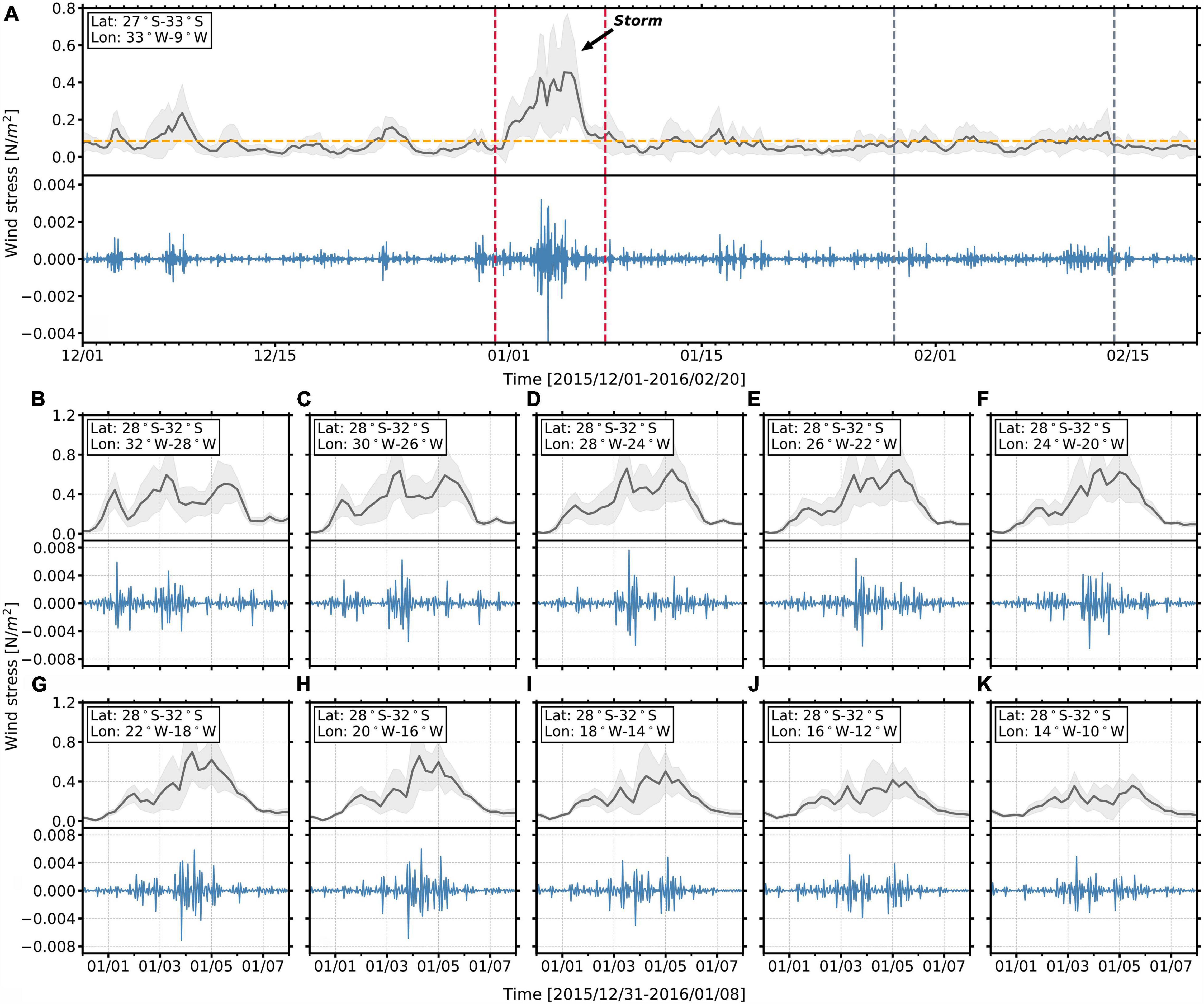
Figure 8. Wind stress variability in time and space. (A) Spatially averaged wind stress as a function of time for region 33° W, 9° W, 27° S, 33° S (upper panel) and its corresponding bandpass filtered near-inertial wind stress (lower panel). Black line = averaged wind stress; blue line = near-inertial wind stress; horizontal dash yellow line = average wind stress for the entire time period. Light gray shade represents the standard deviation of measurements. Vertical red dashed lines bound the time of high wind stress that are analyzed individually as a function of space from panels (B–K). Vertical gray dashed lines bound the days of the seismic survey. (B–K) Same as (A) but for averaged wind stress during the storm analyzed in a series of spatially overlapping windows described in the text. The region of each window is shown in the box at the upper right corner of each figure. The black arrow points to the feature that we interpreted as a storm because its wind stress is greater than eight standard deviations from the mean. Wind stress are calculated from wind speed data from NCEP reanalysis 2 (Kanamitsu et al., 2002).
Over the 60-day period before the seismic survey, wind stresses greater than 8 standard deviations from the mean occur about 30 days prior to the survey between January 01 and January 08, 2016 (Figure 8A, upper panel). We interpret this high wind stress event as a storm. After linearly interpolating the wind stress on an hourly time grid, we use a Butterworth bandpass filter to extract the wind stress in the near-inertial band of 0.8f-1.2f, where f is the Coriolis frequency. Slight changes of lower and upper bounds of the near-inertial band do not significantly affect the results of this analysis. The storm shows a substantial increase in strength within the near-inertial band compared to the rest of the 60-day period (Figure 8A, lower panel), which indicates the important role of this storm in injecting near-inertial energy into the ocean interior.
We spatially track the storm across the seismic survey location by calculating average wind stress along 30° S with a series of rolling windows. Each window has size 4° × 4° and is centered every 2° from 30° W to 12° W (Figures 8B–K). The movement of the storm correlates with the zonal trends of diffusivities. First, higher wind stresses with higher strength in the near-inertial band are shown from 32° W to 14° W during the time of the storm (Figures 8B–I), consistent with the locations of enhanced mixing in seismic derived diffusivity sections (Figure 5,1A–E). Second, the far eastern end of the seismic survey that is above the MAR (15° W to 12° W) did not experience wind forcing as high as regions further west (Figures 8J,K). Correspondingly, we observe lower diffusivities at this location (Figure 5, from the eastern end of lines 1E,F). We note that weaker wind forcing and lower diffusivities at both sides of the MAR provide additional support to our interpretation above - enhanced mixing directly above the MAR is caused by rough topography. The enhanced mixing on lines 1A–E is likely caused by this storm for three reasons: (i) there were no other wind stress peaks within the relevant time range, (ii) enhanced diffusivities track the movement of the storm, and (iii) this region is away from topographic boundaries.
Argo-derived diffusivities support our hypothesis of storm-induced mixing (Figures 1, 9). Argos a, b, c, d were selected because they are within the region of the storm during the time span of the analysis. All Argos show enhanced mixing over a depth range of 300–600 m after wind forcing (Figure 9, red shading), although the timing and strength of these changes vary substantially. Argo a experienced a relatively high level of mixing throughout the time of our analysis. The reason of higher diffusivity of 8.1 × 10⁻⁵ m2 s–1 before the storm is unknown, however, there is a noticeable increase of mixing from 3.9 × 10⁻⁵ m2 s–1 to 9.9 × 10⁻⁵ m2 s–1 after the storm around January 15, then diffusivities maintained above the level of 5.2 × 10⁻⁵ m2 s–1. Argo b shows enhanced mixing during and after the storm, diffusivities increased significantly from 2.4 × 10⁻⁵ m2 s–1 to 23 × 10–5 m2 s–1 in the time of December 26 to January 15. Argo c and d show enhanced mixing during the storm but diffusivities decrease immediately afterward. We also notice a significant increase of diffusivities in Argo a, b, and c about 50, 60, and 30 days after the storm, respectively, while there was no apparent increase in wind stress during these periods of time (Figure 8A). There are two possible reasons for the differences. The first is out of plane effects and the second is local mesoscale flows. While we analyze the diffusivities as a function of time, Argo floats change their spatial location. All floats traveled about 100 km during the time span of analysis (Figure 10). Their Lagrangian behavior means that the diffusivities in Figure 9 do not reflect changes in time at a fixed location. Therefore, other oceanic processes may affect the recovered diffusivities. For example, energy from other events such as wave-wave interactions and near-inertial waves propagating in from elsewhere can have effects on the observed mixing pattern (Plueddemann and Farrar, 2006). However, it is beyond the scope of this contribution to account for out-of-plane influences.
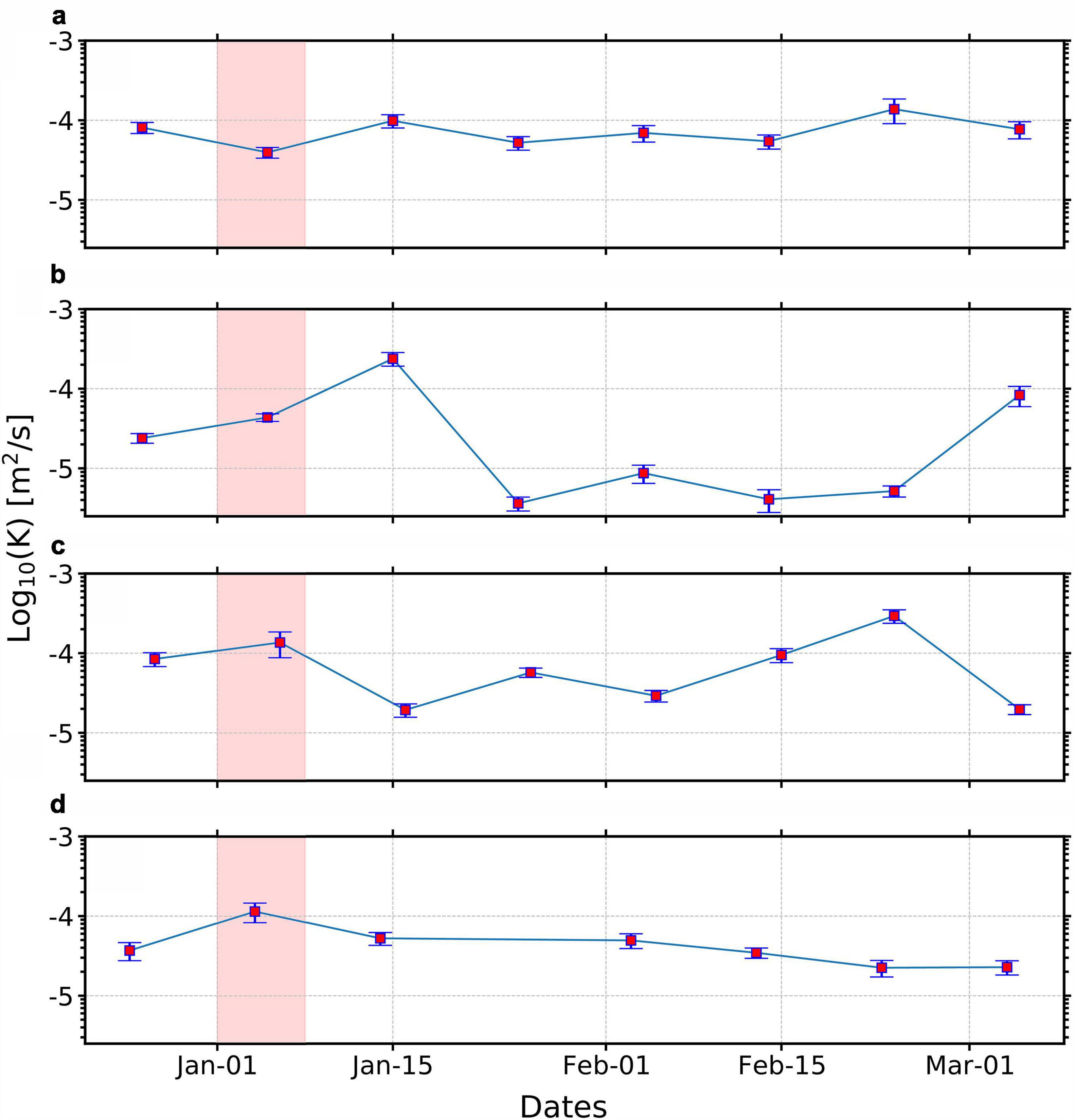
Figure 9. Depth (300–600 m) averaged diffusivity from Argo floats (a–d) as a function of time during and after the storm. Vertical red bands mark the time of the storm. Error bars represent standard errors.
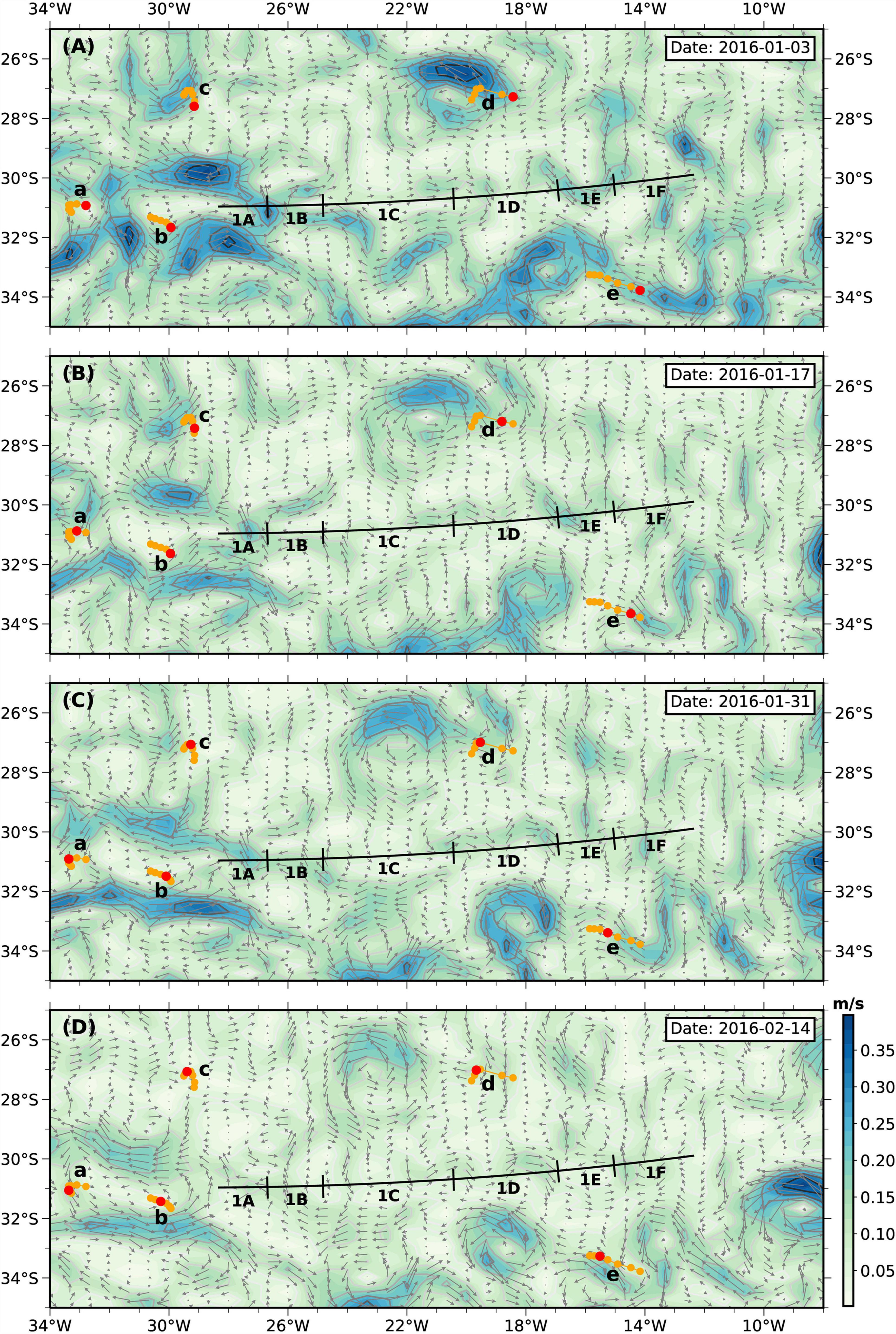
Figure 10. (A) Maps of sea surface geostrophic current velocities calculated for 5 days composite centered on 2016/01/03 from Ocean Surface Current Analyses Real-time (OSCAR) satellite measurements. Black lines = seismic survey lines. Orange dots = the trajectory of the Argo floats a–e shown in Figure 1. Red dots = the positions of the Argo floats closest to the date of the satellite measurements. (B–D) Same as (A) but separated 2 weeks apart following (A).
On the other hand, local mesoscale processes may cause differences between the distribution of ocean mixing and the presence of wind stress at the sea surface. For example, the presence, or lack thereof, of mesoscale eddies has been shown to play an important role in controlling downward propagation of near-inertial energy (Zhai et al., 2005), resulting in different speeds of downward propagation at different times and locations. From the seismic data, we use the different depths of enhanced mixing (Figure 5) and a period of 30 days to calculate the downward propagation speeds of near-inertial energy and find a large range of 17–27 m/day. Furthermore, mismatches between the patterns of wind stress and diffusivities suggest that local mesoscale flows are playing a role in distributing near-inertial energy. For example, the western end of the seismic survey (line 1A) shows the lowest diffusivities while the wind stress was high (Figure 8B). Similarly, we observe diffusivities slightly higher than the background level between 22° W and 20° W (Figure 6), but the wind stress around this region shows sharp spikes in the near-inertial band (Figures 8G,H). Since this region hosts an energetic eddy field, we now consider the possible impact of mesoscale eddies in the mixed layer on propagation of wind-induced near-inertial energy.
Possible Contribution of Eddies
We use satellite observations of sea surface geostrophic current velocities to investigate mesoscale eddies in the mixed layer during the time of the storm. Figure 10 shows the evolution of sea surface geostrophic current velocities from January 03, 2016 to February 14, 2016, covering the time period from the start of the storm to the end of the seismic survey (each plot is separated by 2 weeks). An anticyclonic eddy, centered around 30° W, 31° S and identified by high velocities of ∼0.35 m s–1, is present during the storm. The intensity of the eddy weakens as time goes by Figures 10A–D. The eastern and western portions of seismic lines 1A,B, respectively, cross the easterly side of the eddy. Here, we observe enhanced mixing that propagates to depths greater than ∼800 m in line 1B (Figure 6,1B). The convergence of high velocity currents at this location suggests more complex structures of mesoscale flows compared to other locations (Figure 10A), which could be an explanation for the deeper penetration of enhanced mixing in line 1B. If we consider the eastern edge of the eddy as the input location of deep propagating energy, the location of the deepest penetration is at 50–100 km in line 1B, implying near-inertial energy propagates both vertically and laterally. These findings are consistent with limited previous observations (Jing et al., 2011; Whalen et al., 2018) and numerical studies (Danioux et al., 2008) that reveal the importance of mesoscale eddies in draining energy to great depths. Taken together, these observations suggest that mesoscale eddies enhance the depth-penetration of wind-induced mixing from 600 to 800 m.
To summarize, we hypothesize that wind generated near-inertial energy is a likely candidate for the enhanced mixing away from rough topography, with surface mesoscale flows playing an important role. The enhanced diffusivities we observe are higher than the background level by an order of magnitude in some cases. If our hypothesis of wind-induced mixing holds true, given that the seismic survey was conducted in a non-stormy season, our results demonstrate that wind-induced mixing plays an important role in the central South Atlantic thermocline diffusivities.
Conclusion
We map vertical diffusivities across 1,600 km of the central South Atlantic thermocline using six seismic reflectivity sections, CTD, and Argo data. Seismic reflectivity yields continuous high-resolution diapycnal diffusivity maps of the thermocline during February 2016. These data help to overcome observational limitations since they yield full-thermocline vertical sections that have a horizontal extent of 1,600 km length, vertical and horizontal resolution of O(10) m, and that span a period of 4 weeks. Meanwhile, CTD data from 2003 and 2011 provide low spatial resolution diffusivity estimates that can be seen as representative of the time mean. Argo data provide spot measurements and Lagrangian tracers of mixing over different topographic settings and at different times. Together, these data extend the observational record of diapycnal mixing in the ocean interior and provide insights into the variability and drivers of mixing.
The South Atlantic thermocline is seismically imaged as an 800–900 m band of reflectivity with no clear submesoscale patterns within it (Figure 4). Seismic-derived and CTD-derived diffusivities show that, in the mean, thermocline diffusivities have remained relatively consistent at close to or less than 1 × 10⁻⁵ m2 s–1 since the 1990s (Figures 5, 6). We find low/high diffusivities over smooth/rough topography, and these values are particularly enhanced over the Mid-Atlantic Ridge (25–50 × 10–5 m2 s–1). Imprinted upon the synoptic scale mean, mixing is heterogeneous, showing enhanced diffusivities that exceed the background level of 1 × 10⁻⁵ m2 s–1 in many regions where reflections are weaker and disrupted (Figures 5–7).
We examined the most likely drivers of mixing variability (Figures 8–10). Above the Mid-Atlantic Ridge, diffusivities are enhanced by barotropic tides impinging on the rough bathymetry of the ridge. The rapid decay of diffusivities within ∼30 km away from the ridge implies local dissipation of tidal energy. Above smooth topography, we hypothesize that with limited hydrographic data, we cannot fully decipher what caused the enhanced mixing above smooth topography, however, our best assessment suggests it is likely caused by localized wind-generated near-inertial energy (i.e., a storm). The dissipation of such energy during downward propagation resulted in elevated diffusivities ranging from 3 × 10⁻⁵ m2 s–1 to 50 × 10–5 m2 s–1. The loci and depth of energy propagation vary substantially, possibly affected by the surface wind forcing and mesoscale flows in the mixed layer. The maximum depth of enhanced mixing is about 800 m, taking place close to the edge of an anticyclonic eddy, suggesting mesoscale eddies encourage deeper propagation of near-inertial energy.
The interaction between surface wind, mesoscale flows in the mixed layer, and high mode near-inertial waves is a complex process that remains poorly understood. It is beyond the scope of this study to fully explain the heterogeneity of mixing along the entire seismic survey with limited hydrographic measurements. However, high-resolution seismic observations along with concurrent hydrographic and wind measurements provide an opportunity to untangle these mechanisms. More simultaneous observations are needed in the vicinity of rough topography and strong storm forcing regions to improve our understanding of the global mixing budget and to contribute to more accurate ocean circulation and climate models.
Data Availability Statement
Publicly available datasets were analyzed in this study. These data can be found here: Seismic field data are available at the NSF-sponsored Academic Seismic Portal hosted by Lamont-Doherty Earth Observatory (https://www.marine-geo.org/tools/search/entry.php?id=MGL1601). GO-SHIP observations were downloaded from CLIVAR and Carbon Hydrographic Data Office (https://cchdo.ucsd.edu/) for expocodes A10 49NZ20031106 and 33RO20110926. Argo data were downloaded from the Global Argo Data Repository (https://www.ncei.noaa.gov/products/global-argo-data-repository). Ocean Surface Current Analysis Real-time (OSCAR) and NCEP 2 wind speed datasets were extracted from the following ERDDAP website, respectively: https://upwell.pfeg.noaa.gov/erddap/index.html and https://apdrc.soest.hawaii.edu/erddap/index.html.
Author Contributions
JW and RR conceived the research project. JW carried out data analysis with guidance and wrote the manuscript with contributions from KG and RR. All authors contributed to the article and approved the submitted version.
Funding
CREST was supported by the National Science Foundation (NSF) grant OCE-1537108 to Texas A&M University.
Conflict of Interest
The authors declare that the research was conducted in the absence of any commercial or financial relationships that could be construed as a potential conflict of interest.
Publisher’s Note
All claims expressed in this article are solely those of the authors and do not necessarily represent those of their affiliated organizations, or those of the publisher, the editors and the reviewers. Any product that may be evaluated in this article, or claim that may be made by its manufacturer, is not guaranteed or endorsed by the publisher.
Acknowledgments
We thank the captain, crew, and science party of cruise MGL1601 of the R/V Marcus G. Langseth for their expert assistance during the CREST cruise. We are grateful to W. Fortin for generously providing codes and instructions for calculating high-resolution diffusivity maps. We also thank Q. Tang, K. Sheen, R. Hobbs, J. Estep, H. Potter, R. Hetland, S. Holbrook, and R. Schmitt for their help. Seismic processing was carried out using Seismic Unix (https://github.com/JohnWStockwellJr/SeisUnix) and the Paradigm seismic software applications, Echos, provided by Emerson. Hydrographic measurements were analyzed using the GSW TEOS-10 equation of state for seawater (github.com/TEOS-10/GSW-Python).
References
Alford, M. H. (2003a). Improved global maps and 54-year history of wind-work on ocean inertial motions. Geophys. Res. Lett. 30, 1424–1427. doi: 10.1029/2002GL016614
Alford, M. H. (2003b). Redistribution of energy available for ocean mixing by long-range propagation of internal waves. Nature 423, 159–162. doi: 10.1038/nature01628
Alford, M. H. (2010). Sustained, full-water-column observations of internal waves and mixing near Mendocino Escarpment. J. Phys. Oceanogr. 40, 2643–2660. doi: 10.1175/2010JPO4502.1
Alford, M. H., and Gregg, M. C. (2001). Near-inertial mixing: modulation of shear, strain and microstructure at low latitude. J. Geophys. Res. 106, 16947–16968. doi: 10.1029/2000JC000370
Alford, M. H., Cronin, M. F., and Klymak, J. M. (2012). Annual cycle and depth penetration of wind-generated near-inertial internal waves at Ocean Station Papa in the northeast Pacific. J. Phys. Oceanogr. 42, 889–909. doi: 10.1175/JPO-D-11-092.1
Alford, M. H., MacKinnon, J. A., Simmons, H. L., and Nash, J. D. (2016). Near-inertial internal gravity waves in the ocean. Annu. Rev. Mar. Sci. 8, 95–123. doi: 10.1146/annurev-marine-010814-015746
Bray, N. A., and Fofonoff, N. (1981). Available potential energy for MODE eddies. J. Phys. Oceanogr. 11, 30–47. doi: 10.1175/1520-0485(1981)011<0030:APEFME>2.0.CO;2
Cabré, A., Pelegrí, J., and Vallès-Casanova, I. (2019). Subtropical-tropical transfer in the South Atlantic Ocean. J. Geophys. Res. 124, 4820–4837. doi: 10.1029/2019JC015160
Chaigneau, A., Pizarro, O., and Rojas, W. (2008). Global climatology of near-inertial current characteristics from Lagrangian observations. Geophys. Res. Lett. 35:5. doi: 10.1029/2008GL034060
Danioux, E., Klein, P., and Rivière, P. (2008). Propagation of wind energy into the deep ocean through a fully turbulent mesoscale eddy field. J. Phys. Oceanogr. 38, 2224–2241. doi: 10.1175/2008JPO3821.1
D’Asaro, E. A. (1985). The energy flux from the wind to near-inertial motions in the surface mixed layer. J. Phys. Oceanogr. 15, 1043–1059. doi: 10.1175/1520-0485(1985)015<1043:TEFFTW>2.0.CO;2
D’Asaro, E. A., Eriksen, C. C., Levine, M. D., Niiler, P., and Van Meurs, P. (1995). Upper-ocean inertial currents forced by a strong storm. Part I: data and comparisons with linear theory. J. Phys. Oceanogr. 25, 2909–2936. doi: 10.1175/1520-0485(1995)025<2909:UOICFB>2.0.CO;2
Dickinson, A., Jeremiah White, N., and Patrick Caulfield, C.-C. (2017). Spatial variation of diapycnal diffusivity estimated from seismic imaging of internal wave field, gulf of mexico. JCR Oceans 122, 9827–9854. doi: 10.1002/2017JC013352
Dickinson, A., White, N., and Caulfield, C. (2020). Time-lapse acoustic imaging of mesoscale and fine-scale variability within the faroe-shetland channel. J. Geophys. Res. 125:e2019JC015861. doi: 10.1029/2019JC015861
Dohan, K., and Davis, R. E. (2011). Mixing in the transition layer during two storm events. J. Phys. Oceanogr. 41, 42–66. doi: 10.1175/2010JPO4253.1
Dong, S., Goni, G., and Bringas, F. (2015). Temporal variability of the south atlantic meridional overturning circulation between 20 s and 35 S. Geophys. Res. Lett. 42, 7655–7662. doi: 10.1002/2015GL065603
Estep, J., Reece, R., Kardell, D. A., Christeson, G. L., and Carlson, R. L. (2019). Seismic layer 2a: evolution and thickness from 0-to 70-ma crust in the slow-intermediate spreading south atlantic. J. Geophys. Res. Solid Earth 124, 7633–7651. doi: 10.1029/2019JB017302
Fortin, W. F. J., and Holbrook, W. S. (2009). Sound speed requirements for optimal imaging of seismic oceanography data. Geophys. Res. Lett. 36:L00D01. doi: 10.1029/2009GL038991
Fortin, W. F., Holbrook, W. S., and Schmitt, R. W. (2016). Mapping turbulent diffusivity associated with oceanic internal lee waves offshore Costa Rica. Ocean Sci. 12, 601–612. doi: 10.5194/os-12-601-2016
Fortin, W. F., Holbrook, W. S., and Schmitt, R. W. (2017). Seismic estimates of turbulent diffusivity and evidence of nonlinear internal wave forcing by geometric resonance in the South China Sea. J. Geophys. Res. 122, 8063–8078. doi: 10.1002/2017JC012690
Garrett, C. (2001). What is the “near-inertial” band and why is it different from the rest of the internal wave spectrum? J. Phys. Oceanogr. 31, 962–971. doi: 10.1175/1520-0485(2001)031<0962:WITNIB>2.0.CO;2
Garrett, C., and Munk, W. (1975). Space-time scales of internal waves: a progress report. J. Geophys. Res. 80, 291–297. doi: 10.1029/JC080i003p00291
Garzoli, S. L. (1993). Geostrophic velocity and transport variability in the Brazil-Malvinas Confluence. Deep Sea Res. Part I 40, 1379–1403. doi: 10.1016/0967-0637(93)90118-M
Garzoli, S. L., and Matano, R. (2011). The south atlantic and the atlantic meridional overturning circulation. Deep Sea Res. Part II 58, 1837–1847. doi: 10.1016/j.dsr2.2010.10.063
Gill, A. (1984). On the behavior of internal waves in the wakes of storms. J. Phys. Oceanogr. 14, 1129–1151. doi: 10.1175/1520-0485(1984)014<1129:OTBOIW>2.0.CO;2
Gregg, M. C., Sanford, T. B., and Winkel, D. P. (2003). Reduced mixing from the breaking of internal waves in equatorial waters. Nature 422, 513–515. doi: 10.1038/nature01507
Gunn, K. L., Dickinson, A., White, N., and Caulfield, C.-C. P. (2021). Vertical mixing and heat fluxes conditioned by a seismically imaged oceanic front. Front. Mar. Sci. 8:1379. doi: 10.3389/fmars.2021.697179
Harrison, M., and Hallberg, R. (2008). Pacific subtropical cell response to reduced equatorial dissipation. J. Phys. Oceanogr. 38, 1894–1912. doi: 10.1175/2008JPO3708.1
Hernández-Guerra, A., Talley, L. D., Pelegrí, J. L., Vélez-Belchí, P., Baringer, M. O., Macdonald, A. M., et al. (2019). The upper, deep, abyssal and overturning circulation in the Atlantic Ocean at 30° S in 2003 and 2011. Progr. Oceanogr. 176:102136. doi: 10.1016/j.pocean.2019.102136
Hieronymus, M., Nycander, J., Nilsson, J., Döös, K., and Hallberg, R. (2019). Oceanic overturning and heat transport: the role of background diffusivity. J. Clim. 32, 701–716. doi: 10.1175/JCLI-D-18-0438.1
Hobbs, R. W., Klaeschen, D., Sallarès, V., Vsemirnova, E., and Papenberg, C. (2009). Effect of seismic source bandwidth on reflection sections to image water structure. Geophys. Res. Lett. 36:L00D08. doi: 10.1029/2009GL040215
Holbrook, W. S., Fer, I., Schmitt, R. W., Lizarralde, D., Klymak, J. M., Helfrich, L. C., et al. (2013). Estimating oceanic turbulence dissipation from seismic images. J. Atmos. Oceanic Technol. 30, 1767–1788. doi: 10.1175/JTECH-D-12-00140.1
Jing, Z., Chang, P., DiMarco, S. F., and Wu, L. (2015). Role of near-inertial internal waves in subthermocline diapycnal mixing in the northern Gulf of Mexico. J. Phys. Oceanogr. 45, 3137–3154. doi: 10.1175/JPO-D-14-0227.1
Jing, Z., Wu, L., Li, L., Liu, C., Liang, X., Chen, Z., et al. (2011). Turbulent diapycnal mixing in the subtropical northwestern Pacific: spatial-seasonal variations and role of eddies. J. Geophys. Res. 116:C10028. doi: 10.1029/2011JC007142
Jun, H., Jou, H.-T., Kim, C.-H., Lee, S. H., and Kim, H.-J. (2020). Random noise attenuation of sparker seismic oceanography data with machine learning. Ocean Sci. 16, 1367–1383. doi: 10.5194/os-16-1367-2020
Kanamitsu, M., Ebisuzaki, W., Woollen, J., Yang, S.-K., Hnilo, J., Fiorino, M., et al. (2002). Ncep–doe amip-ii reanalysis (r-2). Bull. Am. Meteorol. Soc. 83, 1631–1644. doi: 10.1175/BAMS-83-11-1631
Klymak, J. M., and Moum, J. N. (2007). Oceanic isopycnal slope spectra. Part II: turbulence. J. Phys. Oceanogr. 37, 1232–1245. doi: 10.1175/JPO3074.1
Klymak, J. M., Moum, J. N., Nash, J. D., Kunze, E., Girton, J. B., Carter, G. S., et al. (2006). An estimate of tidal energy lost to turbulence at the Hawaiian Ridge. J. Phys. Oceanogr. 36, 1148–1164. doi: 10.1175/JPO2885.1
Krahmann, G., Papenberg, C., Brandt, P., and Vogt, M. (2009). Evaluation of seismic reflector slopes with a Yoyo-CTD. Geophys. Res. Lett. 36:L00D02. doi: 10.1029/2009GL038964
Kunze, E., and Toole, J. M. (1997). Tidally driven vorticity, diurnal shear, and turbulence atop Fieberling Seamount. J. Phys. Oceanogr. 27, 2663–2693. doi: 10.1175/1520-0485(1997)027<2663:TDVDSA>2.0.CO;2
Kunze, E., Firing, E., Hummon, J. M., Chereskin, T. K., and Thurnherr, A. M. (2006). Global abyssal mixing inferred from lowered ADCP shear and CTD strain profiles. J. Phys. Oceanogr. 36, 1553–1576. doi: 10.1175/JPO2926.1
Large, W., and Pond, S. (1981). Open ocean momentum flux measurements in moderate to strong winds. J. Phys. Oceanogr. 11, 324–336. doi: 10.1175/1520-0485(1981)011<0324:OOMFMI>2.0.CO;2
Ledwell, J., Montgomery, E., Polzin, K., Laurent, L. S., Schmitt, R., and Toole, J. (2000). Evidence for enhanced mixing over rough topography in the abyssal ocean. Nature 403:179. doi: 10.1038/35003164
Li, Y., and Xu, Y. (2014). Penetration depth of diapycnal mixing generated by wind stress and flow over topography in the northwestern Pacific. J. Geophys. Res. 119, 5501–5514. doi: 10.1002/2013JC009681
Lumpkin, R., and Speer, K. (2007). Global ocean meridional overturning. J. Phys. Oceanogr. 37, 2550–2562. doi: 10.1175/JPO3130.1
MacKinnon, J., and Winters, K. (2005). Subtropical catastrophe: significant loss of low-mode tidal energy at 28.9°. Geophys. Res. Lett. 32:L15605. doi: 10.1029/2005GL023376
MacKinnon, J., St Laurent, L., and Garabato, A. C. N. (2013). Diapycnal mixing processes in the ocean interior. Int. Geophys. 103, 159–183. doi: 10.1016/B978-0-12-391851-2.00007-6
Mauritzen, C., Polzin, K., McCartney, M., Millard, R., and West-Mack, D. (2002). Evidence in hydrography and density fine structure for enhanced vertical mixing over the Mid-Atlantic Ridge in the western Atlantic. J. Geophys. Res. 107, 11-11–11-19. doi: 10.1029/2001JC001114
Mojica, J. F., Sallarès, V., and Biescas, B. (2018). High-resolution diapycnal mixing map of the Alboran Sea thermocline from seismic reflection images. Ocean Sci. 14, 403–415. doi: 10.5194/os-14-403-2018
Munk, W., and Wunsch, C. (1998). Abyssal recipes II: energetics of tidal and wind mixing. Deep Sea Res. Part I 45, 1977–2010. doi: 10.1016/S0967-0637(98)00070-3
Nandi, P., Holbrook, W. S., Pearse, S., Páramo, P., and Schmitt, R. W. (2004). Seismic reflection imaging of water mass boundaries in the Norwegian Sea. Geophys. Res. Lett. 31:L23311. doi: 10.1029/2004GL021325
Osborn, T. (1980). Estimates of the local rate of vertical diffusion from dissipation measurements. J. Phys. Oceanogr. 10, 83–89. doi: 10.1175/1520-0485(1980)010<0083:EOTLRO>2.0.CO;2
Osborn, T. R., and Cox, C. S. (1972). Oceanic fine structure. Geophys. Fluid Dyn. 3, 321–345. doi: 10.1080/03091927208236085
Plueddemann, A., and Farrar, J. (2006). Observations and models of the energy flux from the wind to mixed-layer inertial currents. Deep Sea Res. Part II 53, 5–30. doi: 10.1016/j.dsr2.2005.10.017
Pollard, R. T. (1970). On the generation by winds of inertial waves in the ocean. Deep Sea Res. 17, 795–812. doi: 10.1016/0011-7471(70)90042-2
Polzin, K., Toole, J., Ledwell, J., and Schmitt, R. (1997). Spatial variability of turbulent mixing in the abyssal ocean. Science 276, 93–96. doi: 10.1126/science.276.5309.93
Price, J. F., Weller, R. A., and Pinkel, R. (1986). Diurnal cycling: observations and models of the upper ocean response to diurnal heating, cooling, and wind mixing. J. Geophys. Res. 91, 8411–8427. doi: 10.1029/JC091iC07p08411
Ruddick, B. (2018). Seismic oceanography’s failure to flourish: a possible solution. J. Geophys. Res. 123, 4–7. doi: 10.1002/2017JC013736
Ruddick, B., SoNg, H., Dong, C., and Pinheiro, L. (2009). Water column seismic images as maps of temperature gradient. Oceanography 22, 192–205. doi: 10.5670/oceanog.2009.19
Ryan, W. B., Carbotte, S. M., Coplan, J. O., O’Hara, S., Melkonian, A., Arko, R., et al. (2009). Global multi-resolution topography synthesis. Geochem. Geophys. Geosyst. 10:Q03014. doi: 10.1029/2008GC002332
Sallarès, V., Biescas, B., Buffett, G., Carbonell, R., Dañobeitia, J. J., and Pelegrí, J. L. (2009). Relative contribution of temperature and salinity to ocean acoustic reflectivity. Geophys. Res. Lett. 36:6. doi: 10.1029/2009GL040187
Sheen, K., White, N., and Hobbs, R. (2009). Estimating mixing rates from seismic images of oceanic structure. Geophys. Res. Lett. 36:L00D04. doi: 10.1029/2009GL040106
Simmons, H. L. (2008). Spectral modification and geographic redistribution of the semi-diurnal internal tide. Ocean Modelling 21, 126–138. doi: 10.1016/j.ocemod.2008.01.002
Sloyan, B. M. (2005). Spatial variability of mixing in the Southern Ocean. Geophys. Res. Lett. 32:L18603. doi: 10.1029/2005GL023568
Sloyan, B. M., Wanninkhof, R., Kramp, M., Johnson, G. C., Talley, L. D., Tanhua, T., et al. (2019). The global ocean ship-based hydrographic investigations program (GO-SHIP): a platform for integrated multidisciplinary ocean science. Front. Mar. Sci. 6:445. doi: 10.3389/fmars.2019.00445
St Laurent, L. C., and Thurnherr, A. M. (2007). Intense mixing of lower thermocline water on the crest of the Mid-Atlantic Ridge. Nature 448:680. doi: 10.1038/nature06043
St. Laurent, L. C., Toole, J. M., and Schmitt, R. W. (2001). Buoyancy forcing by turbulence above rough topography in the abyssal Brazil Basin. J. Phys. Oceanogr. 31, 3476–3495. doi: 10.1175/1520-0485(2001)031<3476:BFBTAR>2.0.CO;2
Stramma, L., and England, M. (1999). On the water masses and mean circulation of the South Atlantic Ocean. J. Geophys. Res. 104, 20863–20883. doi: 10.1029/1999JC900139
Tang, Q., Gulick, S. P., Sun, J., Sun, L., and Jing, Z. (2019). Submesoscale features and turbulent mixing of an oblique anticyclonic eddy in the Gulf of Alaska investigated by marine seismic survey data. J. Geophys. Res. 125:e2019JC015393. doi: 10.1029/2019JC015393
Tang, Q., Jing, Z., Lin, J., and Sun, J. (2021). Diapycnal mixing in the subthermocline of the mariana ridge from high-resolution seismic images. J. Phys. Oceanogr. 51, 1283–1300. doi: 10.1175/JPO-D-20-0120.1
Tang, Q., Xu, M., Zheng, C., Xu, X., and Xu, J. (2018). A locally generated high-mode nonlinear internal wave detected on the shelf of the northern south china sea from marine seismic observations. J. Geophys. Res. 123, 1142–1155. doi: 10.1002/2017JC013347
Valla, D., Piola, A. R., Meinen, C. S., and Campos, E. (2018). Strong mixing and recirculation in the northwestern Argentine Basin. J. Geophys. Res. 123, 4624–4648. doi: 10.1029/2018JC013907
Walsh, K. J., Camargo, S. J., Knutson, T. R., Kossin, J., Lee, T.-C., Murakami, H., et al. (2019). Tropical cyclones and climate change. Trop. Cyclone Res. Rev. 8, 240–250. doi: 10.1016/j.tcrr.2020.01.004
Waterhouse, A. F., MacKinnon, J. A., Nash, J. D., Alford, M. H., Kunze, E., Simmons, H. L., et al. (2014). Global patterns of diapycnal mixing from measurements of the turbulent dissipation rate. J. Phys. Oceanogr. 44, 1854–1872. doi: 10.1175/JPO-D-13-0104.1
Whalen, C. B., MacKinnon, J. A., and Talley, L. D. (2018). Large-scale impacts of the mesoscale environment on mixing from wind-driven internal waves. Nat. Geosci. 11, 842–847. doi: 10.1038/s41561-018-0213-6
Whalen, C., Talley, L., and MacKinnon, J. (2012). Spatial and temporal variability of global ocean mixing inferred from Argo profiles. Geophys. Res. Lett. 39:L18612. doi: 10.1029/2012GL053196
Yilmaz, Ö (2001). Seismic Data Analysis: Processing, Inversion, And Interpretation Of Seismic Data. Tulsa, OK: Society of exploration geophysicists. doi: 10.1190/1.9781560801580
Young, W., and Jelloul, M. B. (1997). Propagation of near-inertial oscillations through a geostrophic flow. J. Mar. Res. 55, 735–766. doi: 10.1357/0022240973224283
Zhai, X., Greatbatch, R. J., and Zhao, J. (2005). Enhanced vertical propagation of storm-induced near-inertial energy in an eddying ocean channel model. Geophys. Res. Lett. 32:L18602. doi: 10.1029/2005GL023643
Keywords: seismic oceanography, diapycnal diffusivity, mid-ocean ridge, storm, South Atlantic
Citation: Wei J, Gunn KL and Reece R (2022) Mid-Ocean Ridge and Storm Enhanced Mixing in the Central South Atlantic Thermocline. Front. Mar. Sci. 8:771973. doi: 10.3389/fmars.2021.771973
Received: 07 September 2021; Accepted: 09 December 2021;
Published: 20 January 2022.
Edited by:
Qunshu Tang, South China Sea Institute of Oceanology, Chinese Academy of Sciences (CAS), ChinaReviewed by:
Zhao Jing, Ocean University of China, ChinaQingxuan Yang, Ocean University of China, China
Copyright © 2022 Wei, Gunn and Reece. This is an open-access article distributed under the terms of the Creative Commons Attribution License (CC BY). The use, distribution or reproduction in other forums is permitted, provided the original author(s) and the copyright owner(s) are credited and that the original publication in this journal is cited, in accordance with accepted academic practice. No use, distribution or reproduction is permitted which does not comply with these terms.
*Correspondence: Jingxuan Wei, amluZ3h1YW4ud2VpQHRhbXUuZWR1