A Deep Learning Model to Recognize and Quantitatively Analyze Cold Seep Substrates and the Dominant Associated Species

Introduction

Cold seeps have been documented throughout global oceans along both active and passive continental margins (Sibuet and Olu, 1998). The fluids are enriched with reduced compounds from seabed support in distinctive chemoautotrophic ecosystems (Brooks et al., 1984; Kennicutt et al., 1988). Since their discovery in the Gulf of Mexico in 1983 (Paull et al., 1984), cold seep ecosystems have become “hotspots” of deep sea research due to the special lifestyles of animals, unique adaptations to extreme environments, and important roles in global geochemical cycles (Cordes et al., 2009; Joye, 2020). Most active cold seeps are generally characterized with a vast biomass but low diversity and are dominated by large symbiont-bearing invertebrates (Menot et al., 2010). These invertebrates are considered the ecosystem engineers and influence the sediment environment, provide physical structure and modulate geochemistry through oxygenation (pumping) and ion uptake activities (Levin, 2005). To understand the structure and function of cold seep ecosystems, it is essential to comprehensively describe the distribution of the major habitats and epifauna. However, the topography of cold seep areas is usually complex and heterogeneous. Additionally, the epifauna present a patchy distribution as influenced by discontinued and scattered seep points. It is difficult to obtain complete and comprehensive community information in a traditional way (physical collection, such as epibenthic sled, grab, etc.) due to the region’s high randomness and low representation (Levin et al., 2000). Alternatively, Sen et al. (2016) used multibeam backscatter and bathymetry to obtain complete data for cold seeps. Improved camera (MacDonald et al., 2003; Hsu et al., 2018; Sen et al., 2019) and video technologies (Sen et al., 2016) were also applied, but the subsequent data processing was time-consuming and laborious.

Deep learning is considered one of the major breakthroughs in the artificial intelligence over the past decade and has been widely used in multiple fields including image analysis, target detection, and computer version (Han et al., 2020). This method can be divided into three steps. First, the deep neural network is used to automatically extract features from the target. Then, the model is trained using manually annotated datasets. Finally, the trained model is used to identify the target. Compared with error-prone human performances, deep learning has the unique capability of reducing time and workloads while providing higher reliabilities and accuracies (Raphael et al., 2020). Major deep learning models include convolutional neural networks (CNN; Albawi et al., 2017), recurrent (Cho et al., 2014) and recursive neural networks (Goodfellow et al., 2016), and generative adversarial networks (Creswell et al., 2018). The CNN uses convolutions (special linear operations) in at least one layer of the network instead of typical matrix multiplication operations, which is to process data with grid-like structures. Recurrent neural networks are used to process sequential data and can learn nonlinear features of sequences with high efficiencies. The potential use of recurrent neural networks for learning inferences has been successfully applied to networks with data structure inputs. Generative adversarial networks are based on microgenerators and solve problems by learning new samples from the training set. Generative adversarial networks are based on a game theory scenario in which generators must compete with adversaries (discriminators).

With the development of deep learning, an increasing number of target detection and recognition method have been applied to marine research. The CNN is an efficient deep learning model that can be used to extract profile feature information as it can reduce the network structure complexity as well as the number of parameters through local receptive fields, weight sharing, and pooling operations, while also actively extracting high-dimensional features from big data (Chen et al., 2021). CNN image processing was customized by Zuazo et al. (2020) to extract biological information of the bubblegum coral Paragorgia arborea from times series. Elawady (2015) used a CNN to classify deep-sea coral reefs, which could achieve autonomous coral repairing combined with autonomous underwater vehicles. The Fast R-CNN was applied by Huang et al. (2019) to detect and identify marine organisms with three data augmentation methods expanded a small number of samples. Lu et al. (2017) used the “You Only Look Once: YOLO” approach to recognize and track marine organisms including shrimp, squid, crab and shark. While each of these methods has certain advantages, they show weakness for small-sized target identification and accuracies in cold seeps due to the high habitat heterogeneity caused by complex carbonate rocks and dense organism collections. To adapt to the special environment of cold seeps, it is necessary to develop a new algorithm for substrates and epifauna recognition.

When performing multi-scale target detection, traditional algorithms generally use reduced or expanded images as inputs to generate feature combinations that reflect features at different scales (Adelson et al., 1983). The mainstream deep learning networks currently adopt a single high-level feature for detection. However, the reduced pixel information in small targets make them easily lost in the down-sampling processing. The dominant associated species in cold seeps are relatively smaller in size with a greater community density. Embedding the feature pyramid network (FPN; Lin et al., 2017) structure into the Faster R-CNN (Ren et al., 2015) is a potential solution to improve the detection of small and medium-sized targets.

This paper develops a model to accurately identify substrates and the dominant associated species in cold seeps. Image of the Formosa cold seep collected in the South China Sea were used to train and verify the model.

Model Building

Image Collection and Data Set Production

An imaging and laser profiling system mounted on a remotely operated vehicle (ROV) was used to collect a series of adjacent images with geographic coordinates by the R.V. Kexue in 2016. ROV traveled at a speed of 1.5–2 knots and 2–3 meters above the seabed. Nine images per second was shot and these images can distinguish individuals larger than 1 cm. Geographic coordinates and the same object identifier in adjacent images were used to splice an initial mosaic. The mosaic color was finally uniformed to produce the Mosaic (Figure 1A). For the subsequent training experimental data set and model verification, the Mosaic was divided into 19,516 small images (cut by 200 × 200 and removing blank images). The upper part of the Mosaic was manually tagged for the data set and the other parts were used for the model verification experiment. Tagging targets (Figure 1) primarily includes: (1) the dominant associated species [Gigantidas platifrons (G. platifrons) and Munidopsidae], (2) hard substrates (mussel beds, lobster clusters, biological mixing, shell debris, and exposed authigenic carbonates) and soft substrates (reduced sediments and muddy bottom). The classification of substrates is specified in Table 1.

FIGURE 1

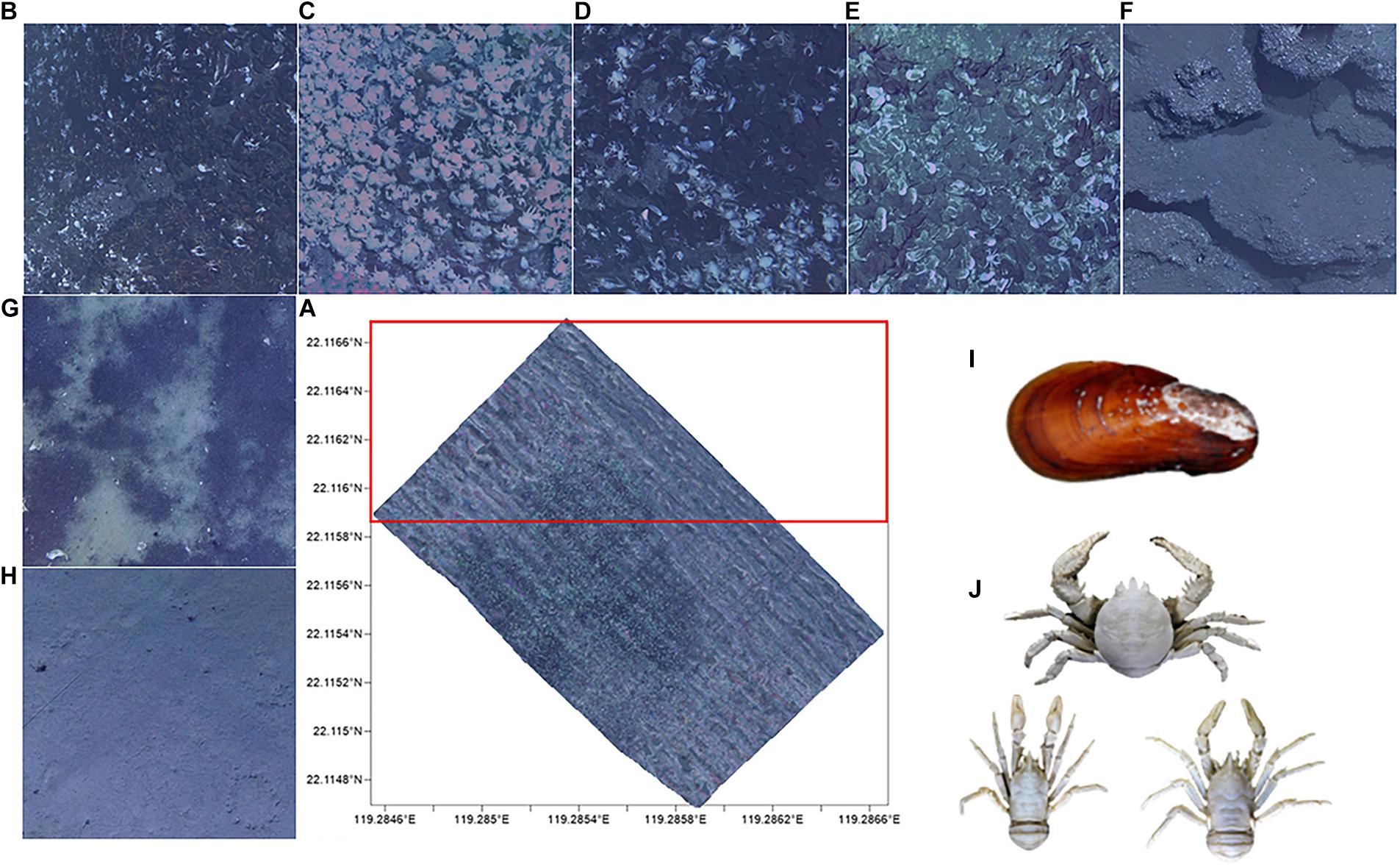
Figure 1. (A) Mosaic (20,000 m²) of Formosa ridge cold seep from 2016. The outline represents the area where images were obtained and the red frame is the training set. The hard substrates are: (B) mussel beds, (C) lobster clusters, (D) biological mixing, (E) shell debris, and (F) exposed authigenic carbonates. The soft substrates are the (G) reduced sediments and (H) muddy bottom. The dominant species in cold seep are (I) Gigantidas platifrons and (J) Munidopsidae.

TABLE 1

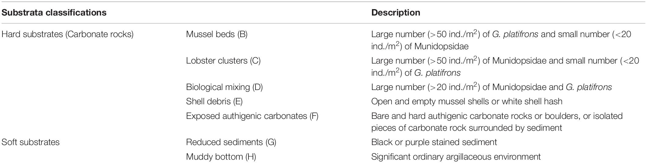
Table 1. Definitions and descriptions of the two main substrates (seven small classifications).

Model Framework

Faster Region-Convolutional Neural Network + Feature Pyramid Network Algorithm for Epifauna Detection

To find an algorithm suitable to detect cold seep epifauna, we considered two-stage (Faster R-CNN base model and our improved model) and single-stage [including SSD300 (Wang et al., 2017) and YOLOv3] detection algorithms to test the same epifauna dataset. The results showed that the two-stage detection model performed better for the average precision (Table 2). Thus, it was more suitable to detect and count cold seep epifauna. However, two-stage detection models are not suitable for real-time target detection because of their relatively lower speeds over single-stage detection. Compared with the original Faster R-CNN structure and other algorithms, the improved algorithm developed in this paper has a higher detection accuracy. Although the detection time increases, the improvement was acceptable relative to the performance. The Fast R-CNN + FPN model was chosen for the recognition of cold seep substrates and epifauna.

TABLE 2

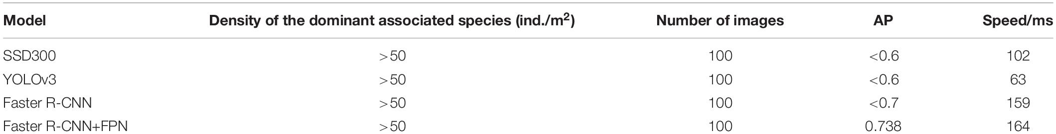
Table 2. The comparison of different models.

The pyramid form of the CNN used in the FPN effectively generates multi-scale feature expressions under a single image view. The FPN structure was designed with a top-down structure while lateral connections fused the shallow high-resolution feature map with the deep feature map having rich semantic information. Embedding the FPN structure in the Faster R-CNN allowed quickly building a feature pyramid with strong semantic information at all scales that could significantly improve the detection capability of the network for small-scale targets (Lin et al., 2017). The FPN structure is showed in Figure 2, where bottom-up usually refers to the forward computing process of the backbone; top-down uses nearest-neighbor interpolation for up-sampling on the higher-level feature map which could retain the semantic information of the feature map to the maximum extent; and the lateral connection adjusts the feature dimension with a 1 × 1 convolution to ensure consistent corresponding feature layer dimensions between the bottom-up process and the top-down processes. Then, the 3 × 3 convolution operation was aimed at eliminating the blending effect generated in the feature fusion process.

FIGURE 2

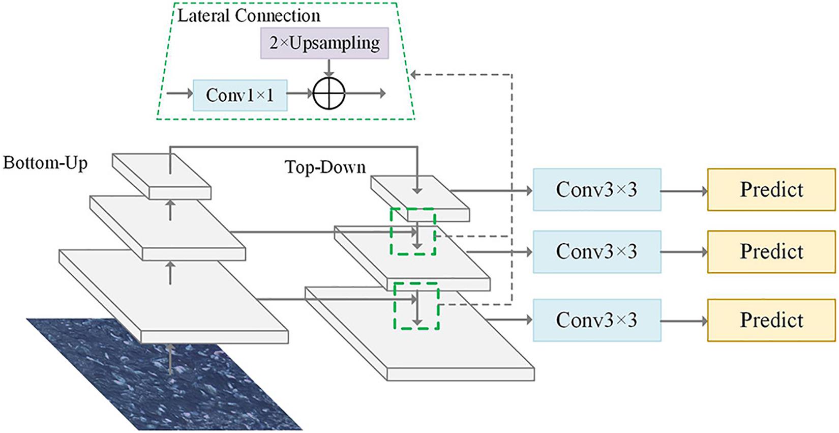
Figure 2. Structure of the feature pyramid network (FPN) algorithm. Top-down structure was designed in the FPN structure while the lateral connections fused the shallow feature map.

Embedding the FPN structure in the Faster R-CNN fused the deep and shallow features, which strengthened the feature expression ability of the network and effectively improved its accuracy for small target detection. In addition, ResNet50 (Szegedy et al., 2017) was used to replace the VGG16 (Simonyan and Zisserman, 2014) as the backbone feature extraction network of the Faster R-CNN to further improve the network capabilities.

The network architecture of the improved Faster R-CNN algorithm is shown in Figure 3. The feature fusion maps for different levels as extracted by the FPN were separately fed into the region proposal network (RPN) network. This network generated anchor frames with different aspect ratios based on the different feature map scale sizes and selected the corresponding detection layer for the target. The region of interest (ROI) pooled the corresponding region into a fixed-size feature vector in the feature map based on the position coordinates of the candidate regions.

FIGURE 3

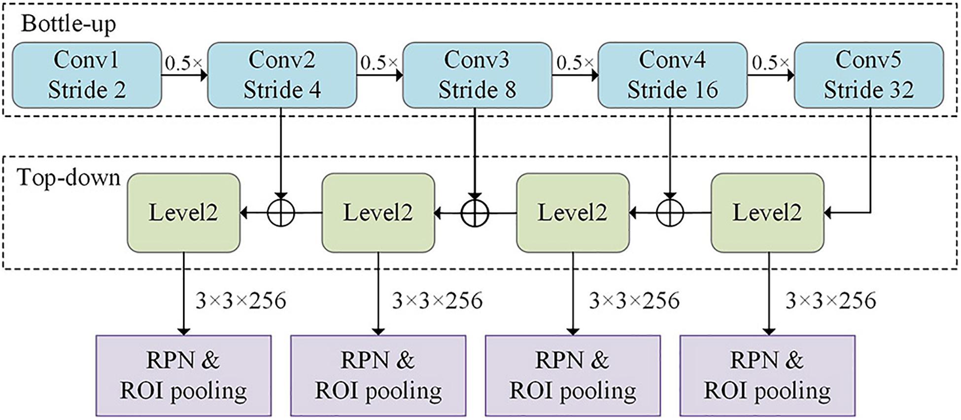
Figure 3. Network architecture of the improved Faster region-convolutional neural network (R-CNN) algorithm, which contains the FPN and region proposal network (RPN).

We set a binary label for each anchor to judge whether it was a target or not to train the RPN. We set a binary label for each anchor to judge whether it was a target or not: we set a positive label for all anchors whose intersection over union (IOU) was greater than or equal to 0.7. We then set a negative labor for all anchors with IOU less than 0.3 for the real box. The loss function of a single image is defined as:

$$\mathit{\text{L}}(\left\{{\mathit{\text{P}}}_{\mathit{i}}\right\},\left\{{\mathit{\text{t}}}_{\mathit{i}}\right\})=\frac{\mathbf{1}}{{\mathit{\text{N}}}_{\mathit{cls}}}\sum _{\mathit{i}}{\mathit{\text{L}}}_{\mathit{cls}}({\mathit{\text{P}}}_{\mathit{i}},{\mathit{\text{P}}}_{\mathit{i}}^{*})+\mathbf{\lambda }\frac{\mathbf{1}}{{\mathit{\text{N}}}_{\mathit{reg}}}\sum _{\mathit{i}}{\mathit{\text{P}}}_{\mathit{i}}^{*}{\mathit{\text{L}}}_{\mathit{reg}}({\mathit{\text{t}}}_{\mathit{i}},{\mathit{\text{t}}}_{\mathit{i}}^{*})$$

where i is the index of the candidate box in a batch of data, P_i is the prediction probability of the i th candidate box as the target. If the candidate box is positive, the real label P_i = 1; otherwise, $P_i^{*}=1$. The λ is the normalized weight with λ=10 set in the experiment, and t_i is the four parameterized coordinate vectors of the prediction box and was the real box vector related to positive samples. The N_cls is the batch size in the training process, N_reg is the number of candidate boxes, and L_cls is the binary logarithm loss and defined as:

$${\mathit{\text{L}}}_{\mathit{cls}}({\mathit{\text{P}}}_{\mathit{i}},{\mathit{\text{P}}}_{\mathit{i}}^{*})=-\mathit{\text{ln}}\left[{\mathit{\text{P}}}_{\mathit{i}}{\mathit{\text{P}}}_{\mathit{i}}^{*}+\left(\mathbf{1}-{\mathit{\text{P}}}_{\mathit{i}}^{*}\right)\left(\mathbf{1}-{\mathit{\text{P}}}_{\mathit{i}}\right)\right]\mathit{\text{s}}$$

The L_reg is the regression loss function and is defined as:

$${\mathit{\text{L}}}_{\mathit{reg}}({\mathit{\text{t}}}_{\mathit{i}},{\mathit{\text{t}}}_{\mathit{i}}^{*})=\sum _{\mathit{i}\in |\mathit{x},\mathit{y},\mathit{w},\mathit{h}|}\mathit{\text{smooth}}({\mathit{\text{t}}}_{\mathbf{i}},{\mathbf{\text{t}}}_{\mathit{i}}^{*})$$

where the smooth function is defined as:

$${\mathit{\text{smooth}}}_{\mathit{L1}}\left(\mathit{x}\right)=\{\begin{array}{c}\hfill \mathbf{0.5}{\mathit{\text{x}}}^{\mathbf{2}}\frac{\mathbf{1}}{{\mathrm{\sigma }}^{\mathbf{2}}},|\mathit{x}|\le \frac{\mathbf{1}}{{\mathrm{\sigma }}^{\mathbf{2}}}\hfill \\ \hfill \left|\mathit{x}\right|-\mathbf{0.5},\mathit{others}\hfill \end{array}$$

where x is the error of the border prediction and σ is used to control the smooth area with a values of 3 in the experiment.

Substrates Recognition Algorithm

The complexity of cold seep substrates and the problems of color bias, dark light and blur in underwater images made it difficult to distinguish all substrate categories using a single classifier. This paper adopted an integration strategy to improve the accuracy of recognition and classification accuracies. In the classification, several base classifiers responsible for distinguishing part of the data were connected in series. The undifferentiated data went to the subsequent base classifier to achieve the optimal results in the iteration.

The associated substrate classification model framework is shown in Figure 4. The first classification model was the FPN embedded in the Faster R-CNN to classify and count the biota. The images that did not satisfy the current classification conditions were passed to the next CNN model, which classified the zones of shell debris and exposed authigenic carbonates. Then, the images that did not satisfy these classification conditions continued to the VGG16 model for binary classification which was responsible for identifying the reduced sediment and muddy bottom zones.

FIGURE 4

Figure 4. Substrate classification model framework with the three classifiers of FPN, convolutional neural network (CNN), and VGG16 to identify the cold seep substrates.

The first base of the integrated classifier in the figure consists of the improved Faster R-CNN and FPN from the section “Faster R-CNN + FPN Algorithm for Epifauna Detection.” The backbone network used for feature extraction in the model, which could greatly improve the feature extraction capability was replaced by VGG16 with ResNet50 as fused with the FPN. The first base classifier was mainly responsible for biota classification. The FPN was embedded into the Faster RCNN to reduce the redundant multi-resolution feature map detection from the original structure based on the realization of feature fusion. Nearest-neighbor upsampling was used to fuse the shallow location and deep semantic information of the network. With only a small increase in computational costs, the detection accuracy of the network for multi-scale targets was greatly improved. Classification and identification allowed counting the epifauna. Then, the zones of the lobster cluster, mussel bed and biological mixing were distinguished using the substrate classification rules.

The second base classifier consisted of the CNN which was aimed primarily at the recognition and classification of the shell debris and carbonate rock zones. This structure could reduce the amount of memory occupied by the deep network, effectively reduce the number of network parameters, and alleviate the overfitting problem of the model. As a supervised multilayer learning neural network, the implicit convolutional and pooling layers were the core modules to realize feature extraction in the CNN. The CNN improved the accuracy of the network through frequent iterative training by minimizing the loss function using the gradient descent method and adjusting the weight parameters in the network layer by layer in reverse (Albawi et al., 2017). The low hidden layer of the CNN consisted of alternating convolutional and maximum pooling layers, and the high level was a fully connected layer corresponding to the implicit layer and logistic regression classifier of a traditional multilayer perceptron. The input of the first fully-connected layer was a feature map obtained via feature extraction from the convolutional and subsampling layers. The final output layer was a classifier for the input image using logistic regression, Softmax regression, or support vector machines. In this paper, a Softmax nonlinear classifier was used to identify and classify the zones of shell debris and exposed authigenic carbonates.

The third base classifier was aimed at the recognition and classification of reduced sediments and muddy bottoms. The VGG16 was composed of five convolutional layers, three fully-connected layers, and an output layer. The layers were separated by a maximum pooling layer and a ReLU activation function for all implicit activation units. On one hand, the convolutional layers with larger kernels could reduce the parameters. On the other hand, these were equivalent to more nonlinear mappings which could increase the expressive power of the network (Simonyan and Zisserman, 2014). However, the nonlinear classifier Softmax was still used for identification and classification.

Model Training and Verification

Epifauna Quantitative Identification Experiments

The Faster R-CNN can be divided into two parts: the RPN and Fast R-CNN network. The former is a recommendation algorithm for candidate boxes (proposal), and the latter is based on the position of the box where the associated categories of objects are calculated. The RPN was trained first, and the Fast R-CNN was trained with the output (proposal) of the RPN. Fast R-CNN was fine-tuned and used to initialize the RPN parameters, which gives an iterative cycle.

The experimental data were 630 images (randomly selected from the upper part of the Mosaic), and the MRLabeler v1.4 software was used for annotation. The model could achieve the best effect when the learning rate was 0.001, the weight decay was set to 0.0004, the anchor scaling multiple was set to (8, 16, 32), and the scaling ratio was (0.5, 1, 2). To avoid overfitting, the impulse gradient was used with impulse of 0.9. The entire experiment was conducted on a Linux CentOS 7 server, and two NVIDIA GeForce GTX 1080ti graphics processing units (GPUs) with 12GB of memory were synchronized. The in-depth learning framework was implemented with tensorflow version 1.11.0 on the GPU. During training, the positive samples were labeled with IOU values greater than 0.7 and negative samples for those less than 0.3. The optimal model was saved after training and used to count the test data set.

The results of each experiment were evaluated using the Recall, Precision and Accuracy (AP). The Recall and Precision are defined as:

$$\mathit{\text{Precision}}=\frac{\mathit{\text{TP}}}{\mathit{\text{TP}}+\mathit{\text{FP}}}$$

$$\mathit{\text{Recall}}=\frac{\mathit{\text{TP}}}{\mathit{\text{TP}}+\mathit{\text{FN}}}$$

where the definitions of TP, TN, FP, and FN as shown in Table 3 denotes true-positive, true-negative, false-positive, and false-negative identifications, respectively. The Precision denotes the proportion of all targets predicted to be correct and the Recall denotes the proportion of targets identified by the correct localization to the total number of targets.

TABLE 3

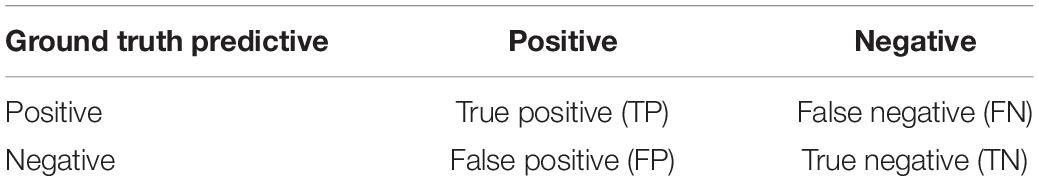
Table 3. Obfuscation matrix for specified categories.

Substrate Identification and Classification Experiments

The MRLabeler v1.4 software was used to label the 1,501 images (randomly selected from the upper part of the Mosaic) in the experimental data set. The specific classification of substrates is shown in Table 1. A total of 303 images were obtained from the biota data set, including 15 images of lobster clusters, 240 images of mussel beds, and 48 images of biological mixing areas. There were 1,198 images of abiotic areas, including 284 of shell debris areas, 107 of exposed authigenic carbonates, 19 of reduced sediments and 788 of muddy bottoms.

The training parameters were set so the first base classifier was the same as the FPN + Faster R -CNN model in the section “Faster R-CNN + FPN Algorithm for Epifauna Detection.” In the second and third base classifiers, the convolution kernel was 3 × 3 and the step size was 1. To ensure optimal performance of each classifier, every detector was trained separately.

Accuracy Verification Experiment

A total of 6,000 images randomly selected from the remaining parts of the Mosaic were used to test the error in the model. The error mean for epifauna was calculated as:

$$\mathit{\text{E}}=\frac{{\sum }_{\mathit{i}}^{\mathit{n}}|\frac{{\mathit{x}}_{\mathit{ir}}-{\mathit{x}}_{\mathit{in}}}{{\mathit{x}}_{\mathit{in}}}|}{\mathit{\text{n}}}$$

where i is the image index, n is the number of images, and x_ir and x_in are the number of epifauna in the images identified by the model and manually counted, respectively. The error mean of the substrates is determined by whether the substrate is correctly identified. The Surfer software was used to show the distribution of substrates and epifauna.

Training and Verification Results and Discussion

Model Training Results

The results show that the Recall, Precision and AP of the Munidopsidae were all greater than the G. platifrons (Table 4). The experimental model training achieved a mean average precision of 73.8% on the epifauna dataset, and the recognition accuracy of G. platifrons and Munidopsidae were 72.0 and 75.6%, respectively. The experimental results are visualized in Figure 5. The experiments indicate that the improved algorithm greatly enhances the accuracy of recognition and counting of cold seep epifauna over other existing methods (Table 2).

TABLE 4

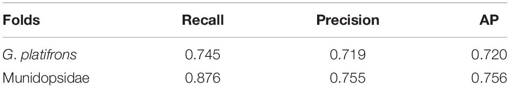
Table 4. Experimental results of the dominant associated species.

FIGURE 5

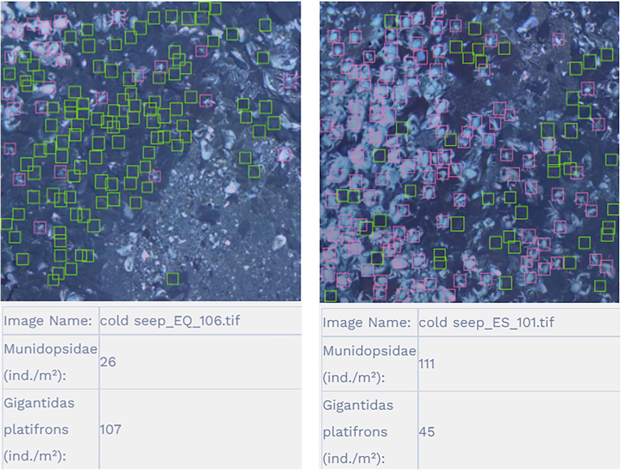
Figure 5. Recognition results for G. platifrons and Munidopsidae as represented as green and pink frames, respectively.

The accuracy of the ensemble classifier was more than 80% (Table 5), and the soft substrates (reduced sediment and muddy bottom) had relatively higher accuracies than hard substrates. Thus, the accuracy of cold seep substrate classification could be greatly improved using the proposed algorithm.

TABLE 5

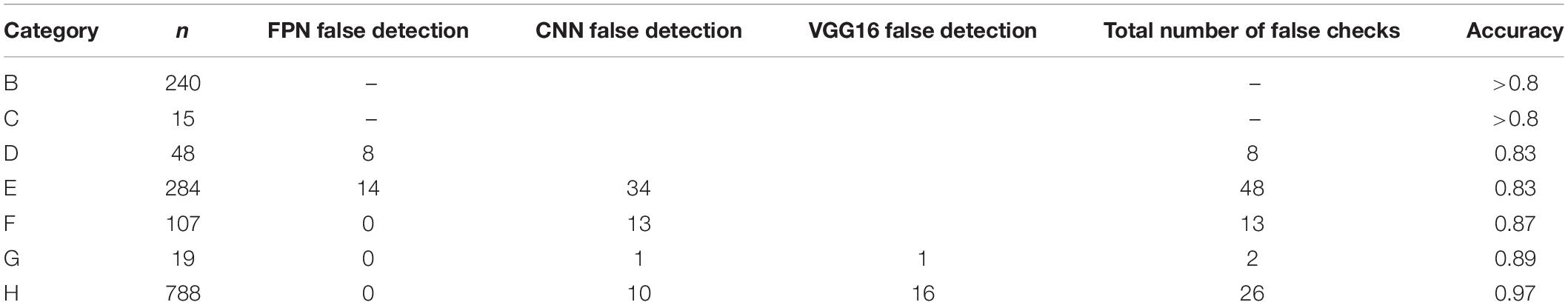
Table 5. Experimental results of the substrates on the test set where (B) to (H) represent the different substrates defined in Table 1.

Model Verification Results

The FPN structure embed into the Faster R-CNN was well adapted to the identification difficulties caused by the particularity of cold seeps. Although single-stage detection algorithms have relatively fast speeds compared with two-stage approaches, these are not suitable for the detection and counting of cold seep epifauna due to the lower average precision. The dominant species (G. platifrons and Munidopsidae) were the main objects of interest. The recognition results indicate that this model weas helpful to detect cold seep epifauna (G. platifrons and Munidopsidae) with a relatively high recognition accuracy (Figure 5). Our study showed that the recognition errors of G. platifrons were lower than Munidopsidae with a range of 0 to 300% and a mean of 29.15%. The recognition errors for Munidopsidae were higher with a range of 0 to 1,650% and a mean of 43.84%. Without calculating the limited epifauna areas, the error means of the two species reached 26.88 and 39.11%, respectively. The different error ranges of G. platifrons were relatively uniform while the Munidopsidae had large differences with concentrations in 0–10 and >50% (Figure 6). Except for the density of 11–20 individual/m² (ind./m²) for Munidopsidae, there were high error means in the range of 0–50 ind./m² for these two species. The error means were all reduced in the range of 50–100 ind./m². The G. platifrons had the lowest error mean for 151–200 ind./m² at 19.37 ± 43.70%, while the Munidopsidae for 81–90 ind./m² had an error of 27.73 ± 24.65%. Both species had low errors at relatively high densities. This also means that our model could meet the needs of cold seep scientific research with dense epifauna. The complexity of cold seep environments and epifauna density were the main reason for changes in the recognition accuracy. The difficulty of identifying G. platifrons was that their shells were similar in color to their surroundings, which created high false positives for the background carbonate rocks. The irregular shape and lamination were the main difficulties for Munidopsidae recognition. The image processing (such as sharpening and contrast stretching) and algorithm still require further improvements.

FIGURE 6

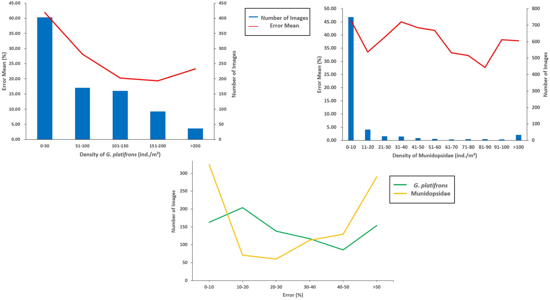
Figure 6. Error mean for different densities about the dominant species and the number of images with different errors.

Several classifiers with different emphases improved the accuracy and interpretability of cold seep substrate classification. Two main substrates (hard and soft) and seven small classifications were defined in Table 1. A total of 480 images of biotas and 5,520 images of abiotic zones were tested, and the error mean of all substrates reached 25.13%. Biological mixing (2.44%), muddy bottom (15.95%), mussel beds (18.54%), and shell debris (28.17%) had relatively lower error means while the exposed authigenic carbonates (40.55%), lobster clusters (51.72%), and reduced sediments (76.30%) had higher error means (Figure 7). The color of the reduced sediments (black and purple) and the exposed authigenic carbonates (gray) were easily confused with the dark surroundings. So, the model may be improved in conjunction with the application of image enhancement technologies.

FIGURE 7

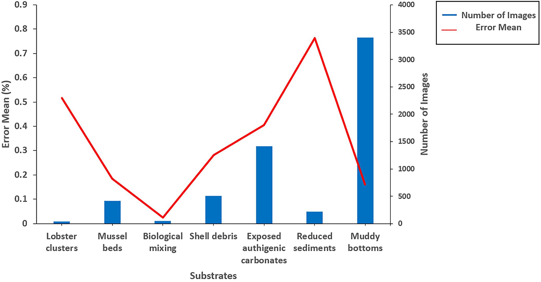
Figure 7. Error means for different substrates.

The recognition and statistical results provide the spatial distribution of substrates and epifaunas in the entire mosaic (Figures 8, 9). Overall, the model identifications of substrates and epifaunas were nearly the same as manual processes. For epifauna, the identification results showed that the total number of G. platifrons and Munidopsidae were 1,75,661 and 24,157 ind. while there were actually 2,15,512 and 37,422 ind., respectively. The identifications in high-density areas were insufficient while some areas with no epifauna showed an excess of false positives. For the substrates, except for the relatively high differences in reduced sediments, the substrate identification was nearly the same as manual operations. The proposed model could be an effective method for the recognition and classification of substrates and epifauna regardless of the number of images.

FIGURE 8

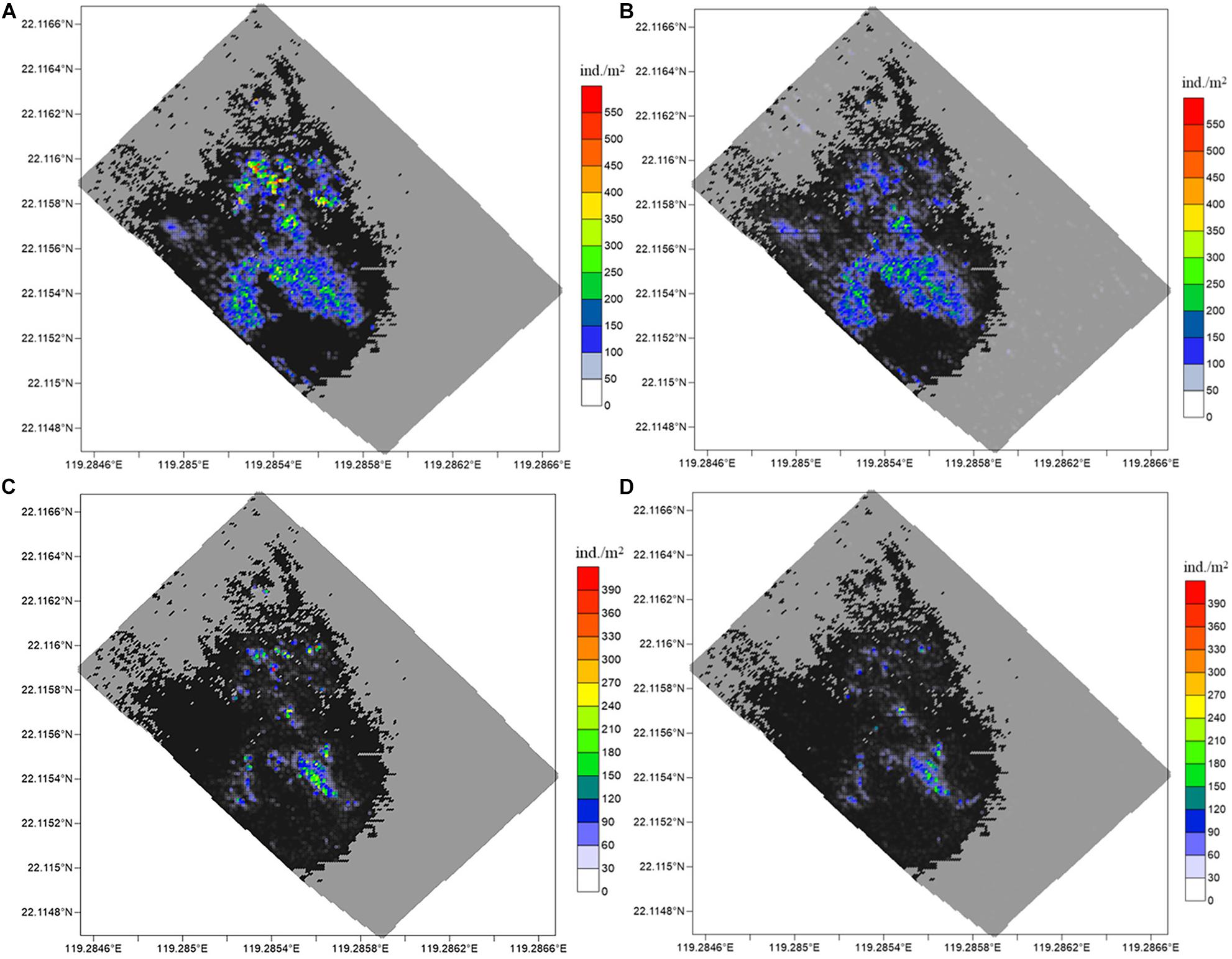
Figure 8. Spatial distribution of G. platifrons and Munidopsidae. The results for G. platifrons with (A) manual counting and (B) model identification, and for Munidopsidae with (C) manual counting and (D) model identification. The large black and gray colored region are hard and soft substrate, respectively.

FIGURE 9

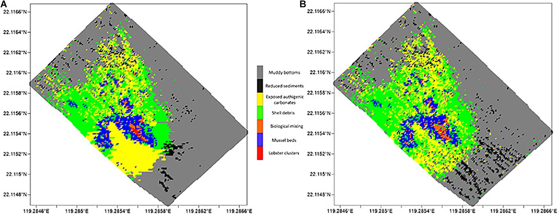
Figure 9. Spatial distribution of different substrates, with (A) manual counting and (B) model identification, respectively.

Conclusion

This paper developed a model to automatically identify and count cold seeps substrates and the dominant associated species. The approach can significantly improve the accuracy of mapping habitats and species distributions, which ensures the sustainable exploitation and utilization of cold seeps. Considering the high heterogeneity of cold seep areas, this will help further cold seep research. The use of the Faster R-CNN + FPN and several integrated classifiers were proven as effective to solve this problem. The classification and recognition of substrates in cold seeps were first applied. To improve the accuracy, future work will focus on image enhancements and algorithm improvements.

Data Availability Statement

Publicly available datasets were analyzed in this study. This data can be found here: doi: 10.12157/IOCAS.20211029.001.

Author Contributions

HW and CL: conceptualization. HW, XF, and ZL: data curation. HW and XF: formal analysis and software and writing—original draft. CL: funding acquisition and writing—review and editing. HW, XF, and CZ: methodology. HW: validation. All authors agreed to be accountable for the content of the work.

Funding

This work was supported by the National Natural Science Foundation of China (42030407 and 42076091), the Strategic Priority Research Program of the Chinese Academy of Sciences (XDA22050303, XDB42020401, and XDA22050302), the National Key R&D Program of the Ministry of Science and Technology (2018YFC0310802), and the Youth Innovation Promotion Association of the Chinese Academy of Sciences. The samples and data were collected by the R.V. Kexue.

Conflict of Interest

The authors declare that the research was conducted in the absence of any commercial or financial relationships that could be construed as a potential conflict of interest.

Publisher’s Note

All claims expressed in this article are solely those of the authors and do not necessarily represent those of their affiliated organizations, or those of the publisher, the editors and the reviewers. Any product that may be evaluated in this article, or claim that may be made by its manufacturer, is not guaranteed or endorsed by the publisher.

Acknowledgments

We thank Bin Zhang and Yuhai Liu for the helping of project implementation. We appreciate the Marine Science Data Center of the Chinese Academy of Sciences for providing data services.

References

Adelson, E. H., Anderson, C. H., Bergen, J. R., Burt, P. J., and Ogden, J. M. (1983). Pyramid methods in image processing. RCA Eng. 29, 33–41.

Google Scholar

Albawi, S., Mohammed, T. A., and Al-Zawi, S. (2017). “Understanding of a convolutional neural network,” in Proceedings of the 2017 International Conference on Engineering and Technology (ICET), Antalya, 1–6.

Google Scholar

Brooks, J. M., Kennicutt, M. C., Fay, R. R., McDonald, T. J., and Sassen, R. (1984). Thermogenic gas hydrates in the Gulf of Mexico. Science 225, 409–411. doi: 10.1126/science.225.4660.409

PubMed Abstract | CrossRef Full Text | Google Scholar

Chen, X., Chen, G., Ge, L., Huang, B., and Cao, C. (2021). Global oceanic eddy identification: a deep learning method from argo profiles and altimetry data. Front. Mar. Sci. 8:646926. doi: 10.3389/fmars.2021.646926

CrossRef Full Text | Google Scholar

Cho, K., Van Merriënboer, B., Gulcehre, C., Bahdanau, D., Bougares, F., Schwenk, H., et al. (2014). “Learning phrase representations using RNN encoder-decoder for statistical machine translation,” in Proceedings of the 2014 Conference on Empirical Methods in Natural Language Processing (EMNLP), Doha, 1724–1734.

Google Scholar

Cordes, E. E., Bergquist, D. C., and Fisher, C. R. (2009). Macro-ecology of gulf of mexico cold seeps. Annu. Rev. Mar. Sci. 1, 143–168. doi: 10.1146/annurev.marine.010908.163912

PubMed Abstract | CrossRef Full Text | Google Scholar

Creswell, A., White, T., Dumoulin, V., Arulkumaran, K., Sengupta, B., and Bharath, A. A. (2018). Generative adversarial networks: an overview. IEEE Signal Process. Mag. 35, 53–65. doi: 10.3115/v1/D14-1179

CrossRef Full Text | Google Scholar

Elawady, M. (2015). Sparse coral classification using deep convolutional neural. Dissertation/master’s thesis, Heriot-Watt University, Scotland (Edinburgh).

Google Scholar

Goodfellow, I., Bengio, Y., and Courville, A. (2016). “Recursive Neural Networks,” in Deep Learning, eds D. Gutierrez and Y. LeCun (Cambridge, MA: MIT press), 400–401.

Google Scholar

Han, F., Yao, J., Zhu, H., and Wang, C. (2020). Marine organism detection and classification from underwater vision based on the deep CNN method. Math. Prob. Eng. 2020, 1–11. doi: 10.1155/2020/3937580

CrossRef Full Text | Google Scholar

Hsu, H.-H., Liu, C.-S., Morita, S., Tu, S.-L., Lin, S., Machiyama, H., et al. (2018). Seismic imaging of the Formosa Ridge cold seep site offshore of southwestern Taiwan. Mar. Geophys. Res. 39, 523–535. doi: 10.1007/s11001-017-9339-y

CrossRef Full Text | Google Scholar

Huang, H., Zhou, H., Yang, X., Zhang, L., Qi, L., and Zang, A.-Y. (2019). Faster R-CNN for marine organisms detection and recognition using data augmentation. Neurocomputing 337, 372–384. doi: 10.1016/j.neucom.2019.01.084

CrossRef Full Text | Google Scholar

Joye, S. B. (2020). The geology and biogeochemistry of hydrocarbon seeps. Annu. Rev. Earth Planet. Sci. 48, 205–31. doi: 10.1146/annurev-earth-063016-020052

CrossRef Full Text | Google Scholar

Kennicutt, M. C., Brooks, J. M., Bidigare, R. R., and Denoux, G. J. (1988). Gulf of Mexico hydrocarbon seep communities—I. Regional distribution of hydrocarbon seepage and associated fauna. Deep Sea Res. Part I Oceanogr. Res. Papers 35, 1639–1651. doi: 10.1016/0198-0149(88)90107-0

CrossRef Full Text | Google Scholar

Levin, L. A. (2005). “Ecology of cold seep sediments: interactions of fauna with flow, chemistry and microbes,” in Oceanography and Marine Biology - An Annual Review, Vol. 43, eds R. N. Gibson, R. J. A. Atkinson, and J. D. M. Gordon (Boca Raton, FL: CRC Press), 1–46. doi: 10.1201/9781420037449.ch1

CrossRef Full Text | Google Scholar

Levin, L. A., James, D. W., Martin, C. M., Rathburn, A. E., Harris, L. H., and Michener, R. H. (2000). Do methane seeps support distinct epifaunal assemblages? Observations on community structure and nutrition from the northern California slope and shelf. Mar. Ecol. Prog. Ser. 208, 21–39. doi: 10.3354/meps208021

CrossRef Full Text | Google Scholar

Lin, T.-Y., Dollár, P., Girshick, R., He, K., Hariharan, B., and Belongie, S. (2017). “Feature pyramid networks for object detection,” in Proceedings of the IEEE conference on computer vision and pattern recognition, San Juan, PR, 2117–2125.

Google Scholar

Lu, H., Li, Y., Uemura, T., Ge, Z., Xu, X., He, L., et al. (2017). FDCNet: filtering deep convolutional network for marine organism classification. Multimed. Tools Appl. 77, 21847–21860. doi: 10.1007/s11042-017-4585-1

CrossRef Full Text | Google Scholar

MacDonald, I. R., Sager, W. W., and Peccini, M. B. (2003). Gas hydrate and chemosynthetic biota in mounded bathymetry at mid-slope hydrocarbon seeps: Northern Gulf of Mexico. Mar. Geol. 198, 133–158. doi: 10.1016/s0025-3227(03)00098-7

CrossRef Full Text | Google Scholar

Menot, L., Galeron, J., Olu, K., Caprais, J.-C., Crassous, P., Khripounoff, A., et al. (2010). Spatial heterogeneity of macrofaunal communities in and near a giant pockmark area in the deep Gulf of Guinea. Mar. Ecol. Evol. Perspect. 31, 78–93. doi: 10.1111/j.1439-0485.2009.00340.x

CrossRef Full Text | Google Scholar

Paull, C. K., Hecker, B., Commeau, R., Freeman-Lynde, R. P., Neumann, C., Corso, W. P., et al. (1984). Biological communities at the Florida Escarpment resemble hydrothermal vent taxa. Science 226, 965–967. doi: 10.1126/science.226.4677.965

PubMed Abstract | CrossRef Full Text | Google Scholar

Raphael, A., Dubinsky, Z., Iluz, D., and Netanyahu, N. S. (2020). Neural network recognition of marine benthos and corals. Diversity 12:29. doi: 10.3390/d12010029

CrossRef Full Text | Google Scholar

Ren, S., He, K., Girshick, R., and Sun, J. (2015). Faster R-CNN: towards real-time object detection with region proposal networks. IEEE Trans. Pattern Anal. Machine Intell. 28, 91–99. doi: 10.1109/TPAMI.2016.2577031

PubMed Abstract | CrossRef Full Text | Google Scholar

Sen, A., Chitkara, C., Hong, W. L., Lepland, A., Cochrane, S., di Primio, R., et al. (2019). Image based quantitative comparisons indicate heightened megabenthos diversity and abundance at a site of weak hydrocarbon seepage in the southwestern Barents Sea. PeerJ 7:e7398. doi: 10.7717/peerj.7398

PubMed Abstract | CrossRef Full Text | Google Scholar

Sen, A., Ondréas, H., Gaillot, A., Marcon, Y., Augustin, J.-M., and Olu, K. (2016). The use of multibeam backscatter and bathymetry as a means of identifying faunal assemblages in a deep-sea cold seep. Deep Sea Res. Part I Oceanogr. Res. Papers 110, 33–49. doi: 10.1016/j.dsr.2016.01.005

CrossRef Full Text | Google Scholar

Sibuet, M., and Olu, K. (1998). Biogeography, biodiversity and fluid dependence of deep-sea cold-seep communities at active and passive margins. Deep Sea Res. Part II Top. Stud. Oceanogr. 45:517. doi: 10.1016/s0967-0645(97)00074-x

CrossRef Full Text | Google Scholar

Simonyan, K., and Zisserman, A. (2014). Very deep convolutional networks for large-scale image recognition. arXiv [Preprint]. arXiv:1409.1556

Google Scholar

Szegedy, C., Ioffe, S., Vanhoucke, V., and Alemi, A. A. (2017). “Inception-v4, inception-resnet and the impact of residual connections on learning,” in Proceedings of the Thirty-First AAAI Conference on Artificial Intelligence, Mountain View, CA, 4278–4284.

Google Scholar

Wang, Y. Y., Wang, C., and Zhang, H. (2017). “Combining single shot multibox detector with transfer learning for ship detection using sentinel-1 images,” in Proceedings of 2017 Sar in Big Data Era: Models, Methods and Applications, Beijing.

Google Scholar

Zuazo, A., Grinyo, J., Lopez-Vazquez, V., Rodriguez, E., Costa, C., Ortenzi, L., et al. (2020). An automated pipeline for image processing and data treatment to track activity rhythms of Paragorgia arborea in relation to hydrographic conditions. Sensors 20:6281. doi: 10.3390/s20216281

PubMed Abstract | CrossRef Full Text | Google Scholar