Assessing the Viability of the Sarasota Bay Community of Bottlenose Dolphins

Introduction

Population Viability Analysis (PVA) is a class of quantitative tools for assessing status, projecting population growth, evaluating threats, and exploring conservation and management options for wildlife populations (Beissinger and McCullough, 2002; Morris and Doak, 2002; Lacy, 2019). PVA usually involves simulation models, in order to consider the many biological, environmental, and human factors and processes that can impact a wildlife population, in a framework that includes consideration of the uncertainties in our knowledge of the system (McGowan et al., 2011), uncertainties about future conditions, and inherent unpredictability of many stochastic biological processes (Lacy, 2000a).

The first applications of PVA were developed to estimate “minimum viable population” size (MVP), the size below which instability of local environments, stochastic demographic processes, disrupted population structure (e.g., Allee effects), genetic decay, and feedbacks among these threats would create a significant threat of population collapse and extinction even if the factors that originally drove the population to small size were ameliorated (Shaffer, 1981; Gilpin and Soulé, 1986). Subsequently, PVA has become a standard tool in conservation and wildlife management (Beissinger, 2002), with the focus on assessing threats and evaluating conservation options. However, applications of PVA are often based on inadequate data to provide confidence in the model projections (Ludwig, 1996; Ralls et al., 2002), and a common recommendation is for PVAs to be used for comparative analyses of threats and options, rather than predictions of population trajectories far into a mostly unknowable future (Reed et al., 2002; McCarthy et al., 2003). Thorough PVAs should include a number of components (Ralls et al., 2002; Lacy, 2019), including:

• Explicit statement of the goals of the analysis, the definition of viability, and the metrics used;

• Documentation (or reference to documentation available elsewhere) of the structure of the PVA model: via using publicly accessible PVA simulation software, providing the software code for custom-made models, or providing detailed description of the model structure and algorithms;

• Description of the values of input parameters (including the sources of data), adequate to allow others to repeat the analyses;

• Explanation of assumptions made in the model structure and estimation of parameter values;

• Consideration of uncertainties in processes modeled (“process uncertainty”) and parameter values (“parameter uncertainty”) – with testing of alternative values, or with incorporation of uncertainties into the model so that the distribution of projected outcomes includes variation due to the uncertainties (McGowan et al., 2011);

• Presentation of not only the mean results but also the variation in results arising from both uncertainties in the inputs and intrinsic environmental and demographic stochasticity (Saether and Engen, 2002);

• Validation that the PVA model generates population structure and dynamics that are consistent with observed population trends.

Population Viability Analysis is most commonly applied to threatened taxa, for which there are concerns about extinction risk, but it is also important to evaluate local populations of wildlife species not currently threatened with extinction. It is often difficult to obtain adequate data on highly threatened species to permit accurate projections with PVA, but data on related, more common species can be used, with appropriate caution, to provide plausible estimates in cases where data gaps hinder analysis of the threatened species (Cervin et al., 2020). Moreover, loss or decline of local populations of even widespread species can damage community and ecosystem structure and function (Ebenman et al., 2004; Gaston and Fuller, 2008). Attention to such processes will be increasingly important as the global environment changes at an accelerating rate (Scheffers et al., 2016). For any population, PVA can serve as a framework for compiling, synthesizing, and documenting what we know and what we do not know about the demography of the population.

The Sarasota Bay common bottlenose dolphin (Tursiops truncatus) community has been studied more intensely and continuously, for more years, than almost any other wildlife population, with research initiated in 1970 (Wells, 2020). These studies provide a more complete picture of the demography of this population than is available for most other species that have been examined with PVA. A few other notable examples of species for which there have been long-term demographic studies that enabled detailed PVA include chimpanzees (Pan troglodytes: Pusey et al., 2007; JGI et al., 2011), red wolves (Canis rufus: Simonis et al., 2018), whooping cranes (Grus americana, Traylor-Holzer, 2019), and the Shark Bay, Australia, population of bottlenose dolphins (T. aduncus: Manlik et al., 2016). Such long-term studies make it possible to build a robust PVA model of the population and validate the model projections against historical trends. With the PVA model, we can examine the current status, project population growth rates, assess tolerance of, or resistance to, threats, test resilience to catastrophic events, quantify sustainable removals or habitat degradation, evaluate management options, and identify needs for research into uncertain parameters that are primary drivers of the populations’ fates. Beyond the significance for the specific population, a PVA of the Sarasota Bay dolphins can provide a template (or baseline for comparison) for examining viability of other populations of small cetaceans.

Materials and Methods

Study Population

The local population that is the focus of this analysis is the long-term resident Sarasota dolphin community, with home range extending through the inshore waters from southern Tampa Bay to Venice Inlet, and to about one kilometer offshore of the Gulf of Mexico beaches (Wells, 2014). For the purposes of this manuscript, the terms population and community are used interchangeably, recognizing that the Sarasota dolphin community is not a closed reproductive unit (Wells et al., 1987). Photographic identification surveys have been conducted through these waters on ten days each month since mid-1992, with a goal of covering the entire area at least three times per month. To increase the probability of capturing life history milestones for dolphins included in the analyses, consideration was limited to those dolphins showing high site fidelity to the core portion of the community home range (Tyson and Wells, 2016). The animal must have had a minimum of 10 sightings recorded since 1975 (or the animal is the calf of a female with at least 10 sightings). Sighting sources included all available data from the sighting database: surveys, focal animal follows, and capture/release. More than 50% of all recorded sightings must lie within the study area as defined above. The animal must have been observed in the region during more than six months of the year. These months can have occurred within 1 year or may have been spread across all of the years of the animal’s records.

Population structure and demographic rates were estimated from the census data for the Sarasota Bay resident community from the full years of 1993 through 2019. Data provided by the Sarasota Dolphin Research Project (Wells, 2020) included records for each individually identifiable dolphin of birth year or year first seen within the population, years of observation within the study population, year of last observation, and a code as to if the disappearance was a known death or unknown if death or emigration. An estimated 95% of dolphins sighted in field surveys were recognizable, so the monitored population consists of most of the resident dolphins. The annual number of newly identifiable dolphins¹ shows that after the initial year (1993), very few previously unknown dolphins other than newborns were added to the catalog of known animals. These newly identified dolphins were treated in the analyses as likely immigrants, although it is possible that some were the result of changes to identifying features, and a few might have been residents that escaped identification for a few years. If a few resident dolphins were missed in annual censuses, the demographic rates and the population projections would still be valid estimates for those dolphins that were monitored. Sample sizes are given in Table 1. Further details of the data collection methods will be given in see text footnote 1.

TABLE 1

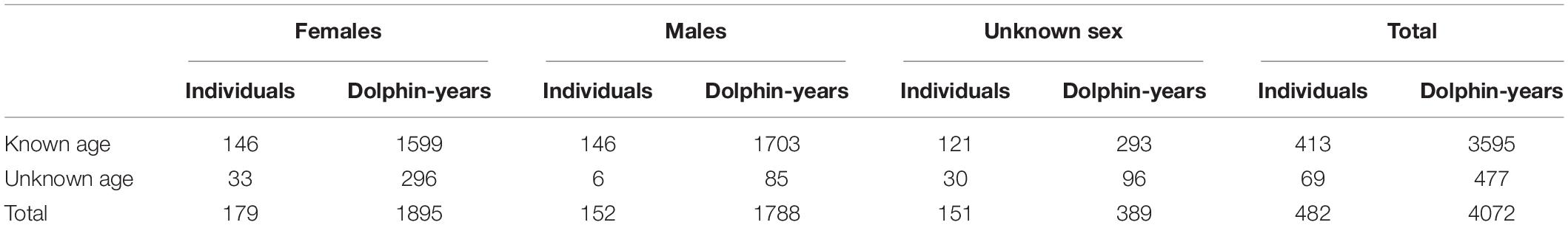
Table 1. Number of individually identifiable dolphins, and dolphin-years of observation, in the Sarasota Bay resident population from 1993 through 2019.

Estimation of Demographic Rates

The census-level data and nearly complete records on the fates of each individual dolphin during those years in which it resided in the study area make possible direct calculations of demographic rates each year and for each age- and sex-class as the number of events (births, disappearances, documented deaths, or arrival into the population as an immigrant) divided by the number of dolphins of that age and sex that were in the population (“at risk” of experiencing the demographic event). Sampling variation in a rate is then given by the standard error for a binomial distribution (Akçakaya, 2002). Age-specific reproductive rates and mortality were calculated on the subset of records for dolphins of known age, with demographic events tallied only for those years that each dolphin was resident in the population (Some dolphins were outside of the community range for intervals of years and resident during other intervals.) In basing the calculations on monitored, individually identifiable animals of known age, we are relying on an assumption that the small number of unidentifiable or unknown age dolphins do not experience different demographic rates than do the monitored individuals. This assumption will be tested by comparing the population projections based on those calculated rates to the observed trends in population size and structure.

For some demographic parameters the most appropriate estimate for use in a PVA model (as described below) can be slightly different than the best estimates used for other purposes. For example, for a PVA model it will likely be unimportant if all females become reproductively mature at the same age (e.g., 6 years) and have lower but increasing reproductive success during their early reproductive years (e.g., up to age 12), or instead each female attains reproductive maturity sometime between 6 and 12 years of age and has the full species-typical reproductive success once it begins breeding. However, that distinction might be important to understanding the life history of the species.

A thorough PVA requires estimates of: mean demographic rates (specified as probabilities of each demographic event – reproduction, mortality, dispersal, etc.); the variation in rates across years; and uncertainty in the model parameters. If there were extreme environmental events with impacts on demography falling outside of the typical variation (“catastrophes”), then the annual variation in each demographic rate can be partitioned into the “environmental variation” (EV) caused by typical fluctuations in the local environment (food, predation, disease, weather) vs. the rates in any catastrophe years. Catastrophe years would then be modeled as a distinct process in a PVA model.

The appropriate breeding and mortality rates to use in the PVA are the means of the observed annual rates, because the simulation model will sample each year a rate from a distribution with that mean and with variance given by EV. Therefore, we obtained means of annual rates by first calculating a rate for each year of data, and then averaging those annual rates (unweighted by annual sample size). If it can be assumed that the true rates are constant across years (i.e., EV = 0), then more precise estimates of mean rates would be obtained by using a weighted mean across years (with the weights being the sample sizes of number of animals monitored each year) – i.e., pooling all data across the years of observation.

Observed annual variation in demographic rates will include both the population-wide variation in probabilities of demographic events (EV) and the inter-individual variation resulting from the fates of individuals being probabilistic outcomes (demographic stochasticity). Therefore, the EV is calculated as the annual variation that exceeds the variation expected as sampling error for a binomial distribution (Akçakaya, 2002). Details of the methodology are given in the Vortex manual (Lacy et al., 2020). The uncertainty in model parameters is normally quantified as the standard error (SE) of the estimates, and this uncertainty can be included in the model projections by sampling the parameter values for each iteration from a normal distribution with the specified mean and SE. Demographic stochasticity is an automatic consequence of an individual-based simulation, in which the fate of each individual is determined by simulating a Bernoulli process (e.g., sex determination, survival vs. death, breeding vs. not, emigration vs. continued residency).

Reproduction

Age-specific reproductive rates were calculated from data on 241 calves for which the age of the dam was known or estimated. In the population model, age of reproduction is defined as the age at which an animal produces a calf. Thus, it is about one year later than conception. The youngest dolphin in the community to produce a calf was 6 years of age. As shown in Figure 1, the proportion of females producing calves increases steadily from age 7 years (about 13% breeding) up to age 12 years (after which about 30% breed each year). From age 12 through 25 years, there was no discernible trend in reproductive rate. After age 25 years, breeding rate steadily decreases, with the oldest known dam being 48 years.

FIGURE 1

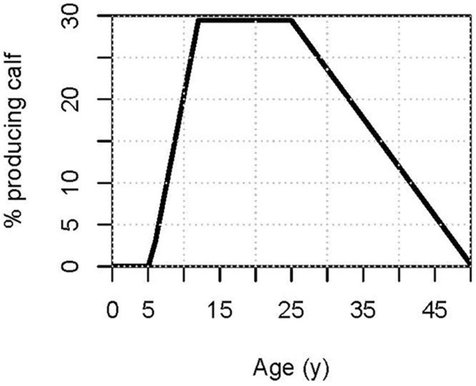
Figure 1. Percent of females of each age producing a calf, as determined from a 3-part regression of breeding rate against age. Equation: %producing calf = 29.42 + 4.399 × (Age-12) × (Age < 12) − 1.165 × (Age-25) × (Age > 25).

We therefore term the age class from 12 to 25 years as the “peak” breeding age. The increasing breeding rate from 6 to 12 years (“young” breeders) is due to different ages of sexual maturation and possibly lower breeding rates among active breeders that are still young. The declining rate after 25 years (“older” breeders) appears to be due to a wide range of ages of reproductive senescence, with previously reproductive females ceasing to reproduce as early as 26 years or as late as 48 years, as well as being due to lower breeding rates in older breeders that were not yet reproductively senescent. The age-specific breeding rate (BR, expressed as the probability of producing a calf in that year) was calculated for the PVA model by a 3-part regression: BR from age 6 to 12 years was calculated as an increasing linear regression; BR from 12 years through 25 years was calculated as a constant (the regression slope was not significant); and the BR from 25 years through 48 years was calculated as a decreasing linear regression. Intercepts of regressions for young (at age 12 years) and older (at age 25 years) females were forced to go through the value estimated for Peak breeding age females. Non-linear regressions did not provide a significantly better fit for any of the three age intervals.

Paternity analysis of 152 calves found that males can breed from age 10 years through 43 years, and this is further supported by analysis of testosterone levels and testis size² (see text footnote 1). Although males in early and late years of the reproductive lifespan appear to sire fewer offspring, for the modeling we assumed no trend with age in the probability of siring a calf. However, the model projections for polygynous species such as bottlenose dolphins do not depend on the proportion of males breeding, unless the population declines to so few males that reproduction is limited by the availability of adult males, or the population is small and closed to immigration and inbreeding occurs due to only a few males siring most of the offspring.

Birth Sex Ratio

The sex is not known for calves that disappeared in the 1st year of life, so the sex ratio at birth is not known with precision. However, of newborns that could be sexed at some time during their lives, there were 86 females and 81 males (120 were unknown sex). We therefore assumed that the birth sex ratio is 1:1.

Mortality

Disappearances of calves less than 1 year of age were assumed to be deaths and not emigration events, even if a carcass was not recovered, because those calves would be unlikely to survive separated from their mothers. For older animals, a disappearance from the resident population could be due to mortality, emigration, or changes to identifying features. Disappearances were recorded as deaths if a carcass was found or if the dolphin was last observed in clearly declining health. Mortality rates for age classes >1 years cannot be calculated directly from the census data, because 66% of disappearances and 59% of disappearances of known age animals could not be documented as deaths. Age-specific loss rates were therefore calculated both for all disappearances and for only known deaths.

It is difficult to estimate emigration rates accurately from the records of dolphins known to have been outside of the study population for intervals of years during which they were known to be alive (due to sightings in nearby populations or later return to residency in Sarasota Bay), because dolphins emigrating permanently from the region would be an unknowable subset that likely had different probabilities of being sighted than did dolphins that remained in nearby populations (whether seen again in the Sarasota Bay community or not). The rate of disappearances is therefore an upper bound, and the documented death rate a lower bound, on the actual mortality rate in the population.

Wells et al. (2015) estimated that 33% of losses are recovered as carcasses, so another estimate of the true death rate is the documented deaths divided by 0.33.

For the purpose of modeling the trajectory of this population, all disappearances represent losses to the community – whether by death or emigration – but these losses will be partly offset by immigrants entering the community. Therefore, we tested scenarios in which all losses were included in the model as “mortality,” and the estimated immigration rate (see section “Immigration” below) was included as an annual input to the population.

After the 1st year, loss and death rates did not vary significantly from year 1 to year 5 (termed “juveniles” for the purpose of this report), nor from year 5 to year 25 (termed “young adults”). A majority of the losses of dolphins in early age classes were unknown sex, so we cannot assess if there is a sex difference in mortality of early ages. The mortality for ages 5 to 25 did not differ significantly between males and females. After year 25 (“older adults”), females and males experienced increased rates of disappearances and of known deaths, and the rates for males increased linearly with age, while older females showed no change in mortality with age. For older males, therefore, the rates at each age were estimated from linear regressions against age, with the intercepts at 25 years being forced to be the mean values for the 6 to 25 years age class.

Maximum Lifespan

The oldest recorded female dolphin in the Sarasota Bay population was 67 years; the oldest recorded male was 52 years (see text footnote 1). In the population model, we specified maximum lifespans of 68 years for females and 53 years for males. The shorter lifespans of males compared to females might be a consequence of the accumulation of PCBs and other persistent organic pollutants in males, while breeding females depurate much of their load of pollutants during gestation and lactation³ (Wells et al., 2005).

Immigration

From 1993 to 2019 there have been 52 dolphins (26 females, 14 males, 12 of unknown sex) that were first observed in the population as subadults or adults and became resident, giving an annual mean of 1.93 immigrants per year. Although the sex ratio among immigrants of known sex is skewed toward females, the sex of a female is more likely to be known, because if they ever produce a calf their sex becomes documented. Thus, we have assumed that the sex ratio of immigrants is 1:1.

Population Modeling

The population dynamics were modeled using the Vortex (version 10.5.5) population viability analysis software (Lacy, 2000b; Lacy and Pollak, 2020; Lacy et al., 2020; software available at www.scti.tools/vortex/). Vortex is an individual-based model that simulates the fate of each individual through an annual cycle of breeding, mortality, increment of age, dispersal among subpopulations, removals (or emigration from the population), supplements (managed or natural immigration), and truncation if the population exceeds the carrying capacity (ceiling density dependence). Stochasticity in demographic processes is modeled as annual variation in each demographic rate at the population level (environmental variation) and random, binomial sampling variation in the fates of individuals (demographic stochasticity) (Lacy, 2000a,b). Vortex provides the flexibility to specify demographic parameters as functions of environmental (e.g., climate, prey base), population (e.g., density, social structure), or individual (e.g., age, contaminant load, location, inbreeding, genotype) properties. Individual fates are summed to provide outputs of projected population sizes (mean, SD, and distribution across independent iterations), population growth rates, population age and sex structure, genetic diversity, and probabilities and times to local extinction or quasi-extinction (N falling below a threshold size).

Population Structure

The starting age and sex structure for the simulations was set to match the census data for identifiable individuals as of 31 December 2019, with 66 females, 61 males, and 33 unknown sex. The unknown sex individuals were assumed to be half females and half males. The 10 resident dolphins of unknown age were assigned an age of 3 years when they arrived in the Sarasota Bay population (6 to 20 years before 2020). These few dolphins all are estimated to be currently mature and not post-reproductive, so their exact ages will have little effect on the population projections. We also tested scenarios that started the simulation with the population structure as it was in 1993. In other scenarios where we tested alternative starting population sizes, we fixed the initial age and sex distribution to match the proportions observed in the current (end of 2019) population.

Other Input Parameters

In addition to the core demographic rates described above, other model input values used in all scenarios are described below.

Reproductive System

Bottlenose dolphins are polygynous, and we assumed no limitation on the number of offspring that a male can sire in a year. All adult males (ages 10 to 43 years) were assumed to be equally likely to sire offspring, resulting in a Poisson distribution of reproductive success among males each year of the simulation.

Correlation Between Annual Variation in Breeding and Survival

The correlation of annual environmental variation (EV) in reproduction and survival was set to 0.5. There is some statistical evidence of a correlation between survival and breeding rate 1 or 2 years later. Breeding was positively correlated with calf mortality 2 years earlier (r = 0.44, P = 0.03), as might be expected if females that lost calves then re-mated the following year. Breeding was negatively correlated with the loss of older females in the prior year (r = −0.50, P = 0.01), with the same trend but non-significant for losses of older males (r = −0.28, P = 0.17) and peak age males and females (r = −0.30, P = 0.13), suggesting that common stresses depressed both survival and reproductive success. However, the estimated EVs for most demographic rates are small, so any correlation specified in this annual variation in rates will have minimal effect on the population trajectories generated by the model.

Inbreeding Depression

Inbreeding depression was not modeled because with a long generation time, a population size greater than 100, and some immigration from other communities, inbreeding would likely remain low, as suggested by Duffield and Wells (2002).

Catastrophes

The option in Vortex to impose sporadic catastrophes was used only for the scenarios in which we examined the resilience of the population to any sudden decline (see below). There were as few as 2 births in 2003, but the count would need to be 0 or 1 to be a statistical outlier in the distribution of births per year (mean = 9.89, SD = 4.40). In 1996 there was a high number of disappearances (13.2%, compared to a mean = 6.5%, SD = 2.4%), but that year had good reproduction. Therefore, all 27 years of data on reproduction and mortality were included in the calculations of EV, rather than partitioning the worst performing years as distinct “catastrophes” in the model.

Carrying Capacity

It is not known how many dolphins could be supported by the Sarasota Bay habitat, or whether this has changed over time. Since 1999, the population has varied from 140 to 184 identifiable resident dolphins, with the highest numbers (176 to 184) in the last 4 years. This suggests that the population might be near its carrying capacity (K); for the modeling we assumed K = 200. Vortex uses a ceiling model of carrying capacity, imposing additional mortality across all age classes whenever the population size exceeds K. An option to include density dependent reproductive success in the model was not implemented, because data are insufficient to allow estimation of the functional relationship between population size and breeding success. Correlations between N and birth rate and between N and each age class mortality rate were all non-significant (P > 0.10).

The population growth rate in the model projections is calculated each year before any truncation of the population to constrain N to be no greater than K, so the limiting K in the simulation affects population size (if the population grows) but does not affect reported growth rate unless K is so low that demographic stochasticity is reducing mean population growth substantially even when N approaches K (This was not the case in our simulations, except in tests of the Minimum Viable Population size).

Time Span of Projections and Number of Iterations

The population trajectory was projected for 100 years, with 5,000 independent iterations of most scenarios. For analyses that partitioned variance among sources of uncertainty (see section “Sensitivity Analyses,” below), 100,000 iterations were run to obtain adequate sample sizes for variance partitioning among the large number of factors.

Output Metrics

Population viability was assessed by the mean exponential growth rate [r = ln(N_t/N_t-₁)] averaged across years and iterations, the variation in growth expressed as SD(r), the final population size (N), and the variation across iterations in N, expressed as SD(N). Population size was tallied in the simulation after all breeding, mortality, immigration, and emigration of the year, and therefore would correspond approximately to the census data on the Sarasota population as of the first of each year. The growth rate, r, was calculated each year of the simulation before any truncation of population size due to the carrying capacity being exceeded; it therefore represents the potential population growth in the absence of population size limitations.

Scenarios Examined

Baseline

To describe and project the resident population with the best estimates of rates and factors controlling the population dynamics, we ran a Baseline scenario with the estimated demographic rates as described above. For each iteration, the values of breeding and mortality rates were sampled from normal distributions with means as described above and SD set to the standard error of each estimate. Thus, the variation in simulation projections will encompass the uncertainty due to imprecision of estimates of demographic rates. Mortality rates in the Baseline were set to the total rates of disappearance, and therefore encompassed both true mortality and losses due to permanent emigration from the population. Immigration into the population was modeled by supplementing the mean immigration rate of 1.93 dolphins per year, with the number of immigrants each year of the simulation sampled from a Poisson distribution. Because less than 1/3 of the immigrants were of known age, for the Baseline simulation we specified the ages of immigrants added to the population by sampling from a uniform distribution from 2 years upwards. Of the 17 immigrants of known age, ages ranged from 2 to 35 years, with a mean of 10 years; however, older immigrants would be less likely to have their ages known, because they would have been adults when first observed.

Validation

This scenario set the initial population size and age structure to be the census population on 1 January 1993, as a test of the accuracy with which the population simulation replicates the observed population growth from 1993 to 2020. Demographic rates were as specified in the Baseline scenario.

Minimum Mortality

This scenario represents the maximum growth rate that might be achieved in a closed population with the estimated birth and death rates. This scenario set the mortality rates to match the rates of documented deaths, and the scenario did not include any immigration.

Estimated Mortality

This scenario assumes that 33% of deaths are recovered as carcasses (as reported in Wells et al., 2015), for all age classes above young of the year. The mortality in the model was set to the rate of documented deaths divided by 0.33, but with each mortality rate capped at the observed total rate of disappearances for that age class. This cap was imposed because in age classes beyond juveniles the rate of disappearances was less than 3 times the death rate. Immigration was not included, so as to represent a plausible estimate of the intrinsic demography of the resident population in the absence of immigration and emigration.

Maximum Mortality

This scenario represents the growth rate that would be achieved in the population if all disappearances were counted as losses (mortality in the model), and the population received no immigrants. This scenario could result either from a closed population in which the losses were all due to death, or a population that loses some emigrants each year but receives no supplementation via immigration from other populations.

Tolerance of Additional Mortality

The tolerance of the dolphin population to increased mortality as might occur due to increased entanglement in fishing gear, more injuries from boat strikes, or other anthropogenic causes was examined in a set of scenarios that set the survival rates for all age classes to be from 95% up to 100% of the mean survival estimated in the past 27 years of census data.

Red Tide

Two scenarios were run to test the impact of severe red tide events on long-term mean population growth. Severe red tides occurred in the Sarasota Bay area in 2005, 2006, and across 2018-2019 (Berens McCabe et al., 2021). Mortality of calves and juveniles was higher in 2006 and 2019 than the average of other years (although not significantly so), and the population declined in 2006 (r = −0.086, a greater decline than in any other year) and in 2019 (r = −0.039). The population growth expected if those 2 years of higher mortality had not occurred was estimated by omitting those 2 years of data from the estimates of mortality rates that were used in the population model. Population growth if red tides become more frequent was projected by duplicating those 2 years of mortality data (calculating rates based on 27 + 2 years of data) for estimation of rates. For older adult males, loss rates were specified to be a function of age, with the rate of loss at age 25 years set to the value for young adults, and the slope as determined from the original 27-year dataset.

Minimum Viable Population

The Sarasota Bay community is not a closed population, so the concept of a minimum viable population (MVP) is not applicable to that population. However, the detailed demographic data available do provide an opportunity to examine what population size might be required for assuring the long-term persistence of a coastal population of dolphins. We tested a range of population sizes from N = 10 to the current N = 160, under the assumption of a closed population with carrying capacity set to the initial size. We set the mortality rates to be those estimated from observed deaths (as in Estimated mortality, above) and included no immigration.

Resilience

The ability of the population to recover from a catastrophic decline such as might be caused by a disease outbreak, harmful algal bloom, or a major spill of oil or other toxic chemicals was examined in scenarios that imposed a catastrophe at the initial year that killed 25%, 50%, or 75% of dolphins across all age classes in what was otherwise the Baseline model. These catastrophe scenarios assumed that the deaths occurred at year 1, and there was no impact on reproduction of surviving dolphins. The effects would be similar if that total number of deaths occurred over several years. The effects of a catastrophe would be exacerbated if there were also impacts on reproduction by the surviving animals.

Sensitivity Analyses

Sensitivity analysis of the impact of variable or uncertain input parameters can be conducted testing a range or set of alternative values, or by sampling parameter values each iteration from specified distributions describing the uncertainties in the true values.

Parameter Uncertainty

The sensitivity of population projections to uncertainty in each model parameter was examined by comparing projections with the value set to the mean −2 SE, −1 SE, baseline, +1 SE, and +2 SE for each parameter.

In addition, in the full Baseline model that includes sampling parameter uncertainty for each iteration (similar to the methods in Caswell et al., 1998; and recommended by Prowse et al., 2016), we used ANOVA to determine the percent of variation in population growth that is due to the uncertainty in each parameter. For this partitioning of causes of variation, we considered uncertainty in population trends at two levels: the variation in long-term mean trajectories (quantified by the mean exponential growth rate, r), and variation in population size from year to year (quantified by the growth rate in a given year). The annual variation in population change will include the possibly large variation due to intrinsic demographic stochasticity and environmental variation, whereas these components of variation will be largely averaged out when long-term means are examined.

Natural Variability

The sensitivity to the variation in demographic rates observed over time (EV) was examined by comparing projections with the value set to mean −2 EV, −1 EV, baseline, +1 EV and +2 EV. In this sensitivity test of annual variation, values of parameters were not sampled from distributions describing the standard errors around mean values, so as to remove that parameter uncertainty from the model when effects of environmental variation were assessed.

In addition, in the Baseline model, demographic rates were sampled each iteration from normal distributions with SD = estimated EV. The effects of the sampled values each year on annual population growth were assessed also by an ANOVA that quantified the percent of variation in annual population growth that was due to the environmental variation in birth and death rates.

Results

Demographic Rates

Breeding Rate

From age 6 to 12 years, breeding rate (BR) fit a linear regression, with BR = 29.42–4.339×(12−AGE) (R² = 0.80, P < 0.001). This regression predicts that only 3.4% of females age 6 years would produce a calf. Since 1993, no females (of 61 of known to have reached 6 years) have produced a calf before 7 years, but one female did so before the detailed monitoring began in 1993. Total annual variation in BR for young adult females was no greater than the predicted binomial sampling variance, so we have no evidence for any environmental variation in BR for young adult females.

The mean breeding rate as a mean of the 27 annual rates for peak age females (age 12 to 25 years) was 29.42%. The residual variation (EV) after removing binomial sampling variation was SD = 7.97%.

From age 26 to 48 years, BR fit a linear regression, with BR = 29.42–1.165×(AGE−25) (R² = 0.25, P < 0.001). This regression predicts that only 2.6% of females of age 48 years would produce a calf. Two of 8 females age 48 years did produce calves, although only 8 births (out of a predicted 7.4 births) occurred to females in age classes 40 to 47 years. EV was estimated as SD = 3.08%.

Table 2 gives the birth rates for the three age categories of females, with standard errors of means, annual variation (given as SD), and the component of variance ascribed to EV. “Pooled (weighted)” rates combined data across all years to calculate overall mean rates. This weights each year’s rate by the sample size for that year. “Mean annual” rates were obtained by first calculating a rate for each year, and then averaging those annual rates (unweighted by annual sample size), for use in the PVA model. Environmental variation (EV) was determined by subtracting the expected binomial sampling variance from the total variance across years. EV = 0 indicates that the total annual variation was no greater than expected from the binomial sampling variance. The three-part regression describing the age-specific birth rate for young (6 to 11 years), peak age (12 to 25 years), and older (26 to 48 years) is shown in Figure 1.

TABLE 2

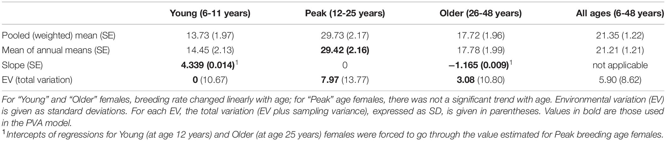
Table 2. Breeding rates, given as percent of females in that age range that produce a calf in an average year.

Mortality Rate

The mean annual mortality of calves within the first 12 months was calculated as 24.10%, with EV calculated to be SD = 6.38%.

The mean annual rate of disappearance for age intervals 1-2 years, 2-3 years, 3-4 years, and 4-5 years was 8.10%, with EV of SD = 2.10%. The mean annual rate of known deaths for age intervals 1-2 years, 2-3 years, 3-4 years, and 4-5 years was 1.83%, with no evidence of EV because the total annual variation did not exceed that expected from the binomial sampling variation (demographic stochasticity).

From year 5 through year 25, the overall mean annual rate of disappearance was 2.58%. The overall mean rate of known deaths was 1.02%. No EV was detected for the rate of either disappearances or known deaths.

For older females above 25 years of age (up to 68 years), the mean annual rate of disappearance was 5.84%. The mean annual rate of known deaths was 3.56%. There was also no detectable EV in mortality of older females.

For older males above 25 years, mortality increased with age. The rate of disappearances fit a linear regression of: Loss Rate (%) = 2.58 + 0.885 × (AGE-25) (R² = 0.255; P < 0.001), with the intercept forced to go through the value estimated for young adults (age 5 to 25 years). The rate of documented deaths fit a linear regression of: Death Rate (%) = 1.02 + 0.451 × (AGE-25) (R² = 0.265; P < 0.01). These regressions were not calculated for mean annual loss and death rates for older adult males, because sample sizes were inadequate to allow estimation of the regression for each year of data. Instead, the values pooled across years were used to estimate the regression. EV was calculated on the rates averaged across ages and was SD = 2.91% and SD = 2.64% for rate of disappearance and of known deaths, respectively.

The overall rate of disappearances of unknown age dolphins was 9.01%. The exclusion of these dolphins from age-specific loss rates might lead to an underestimation of those rates, but the unknown age animals account for less than 10% of the animal-years of data. Moreover, the higher loss rate for unknown age dolphins might be caused by those animals often being older animals (being dolphins first observed as adults), and the loss rate for unknown age animals is approximately the rate predicted for 32 years old males. There were only 3 documented deaths among unknown age dolphins, so excluding those few cases has minimal effect on age-specific death rates.

Table 3 gives the age-specific rates of disappearance and of known deaths, as the mean of annual rates and pooled across years, with standard errors of means, annual variance, and variance ascribed to environmental variation.

TABLE 3

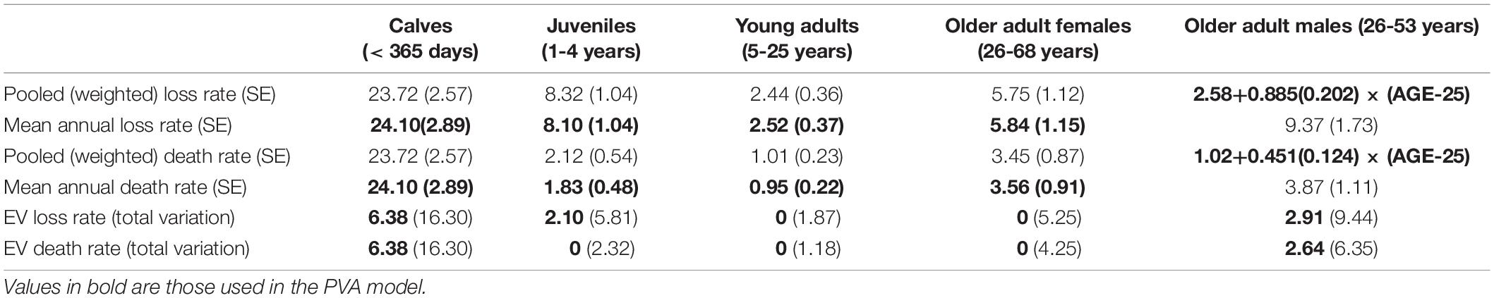
Table 3. Calculated rates of disappearance (“Loss”) and documented deaths with SE in parentheses, and environmental variation in the rates given as SD, with total observed annual variation (EV plus sampling variance) expressed as an SD in parentheses.

Deterministic Population Growth

Table 4 shows the long-term population growth calculated from the mean fecundity and survival rates, following standard deterministic calculations on the life table (Caswell, 2001) for each of several estimates of mortality rates. These estimates omit any immigration and emigration, and therefore represent deterministic population growth intrinsic to the local population. Also shown are the mean generation times for females and males and the stable age distribution for each case. The age distribution is compared to the population census as of 1 January 2020.

TABLE 4

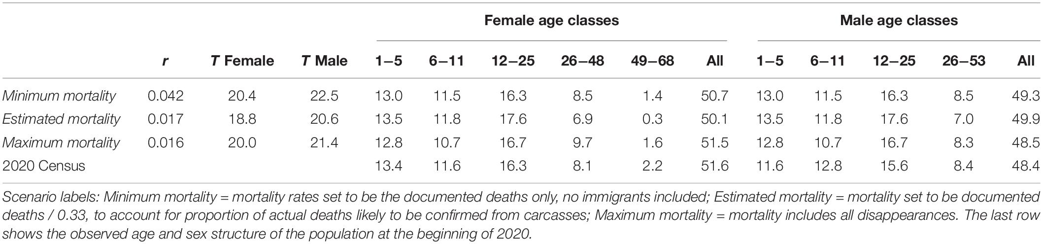
Table 4. Deterministic population growth rate (r), mean generation time (T) for males and females, and stable age distribution (expressed as %), calculated from mean demographic rates.

The Minimum mortality case can result in a mean deterministic population growth rate over 4%, but that case assumes unrealistically that all deaths were documented with recovered carcasses or observation of dying animals and all other disappearances were emigrations that would not be tallied as losses in a life table calculation. The cases with Estimated mortality, based on an estimated 33% of deaths being documented, and Maximum mortality, based on all disappearances being tallied as deaths, produce calculated intrinsic population growth rates of r = 0.017 and r = 0.016, respectively.

Mean generation time (mean age of a parent, weighted to account for diminishing contribution of later offspring in a growing population) is about 2 years longer in males than females, because males mature later. Females can have longer lifespans than males, but they stop breeding before exceeding the maximum age observed for males, so the females reaching the oldest age classes do not contribute to the mean generation time.

The age distribution at the start of 2020 closely matched the stable age distributions calculated with each of the several estimated mortality rates, and both observed and calculated distributions yield a sex ratio close to 50:50.

Validation of the Stochastic Model of Population Dynamics

The ability of the model to simulate accurately the dynamics of the population was examined by comparing projections in the Validation model, when started with the age structure as it was in 1993, to observed census trends from 1993 to 2020. The mean population growth in this Validation scenario of r = 0.019, with SD(r) = 0.035, matched the observed mean population growth from 1993 through 2019 (r = 0.019), but had less variation in growth across years than observed in the censuses (SD(r) = 0.066). Figure 2 shows the observed population size, the mean trajectory in the Validation scenario, and error bars encompassing 95% of the distribution of individual iterations of the simulation. The observed population sizes remained mostly within the range of the simulations, and the censused population at the beginning of 2020 (N = 160) was well within the range of uncertainty of the final population size projected in 2020 (mean N = 175, SD = 36).

FIGURE 2

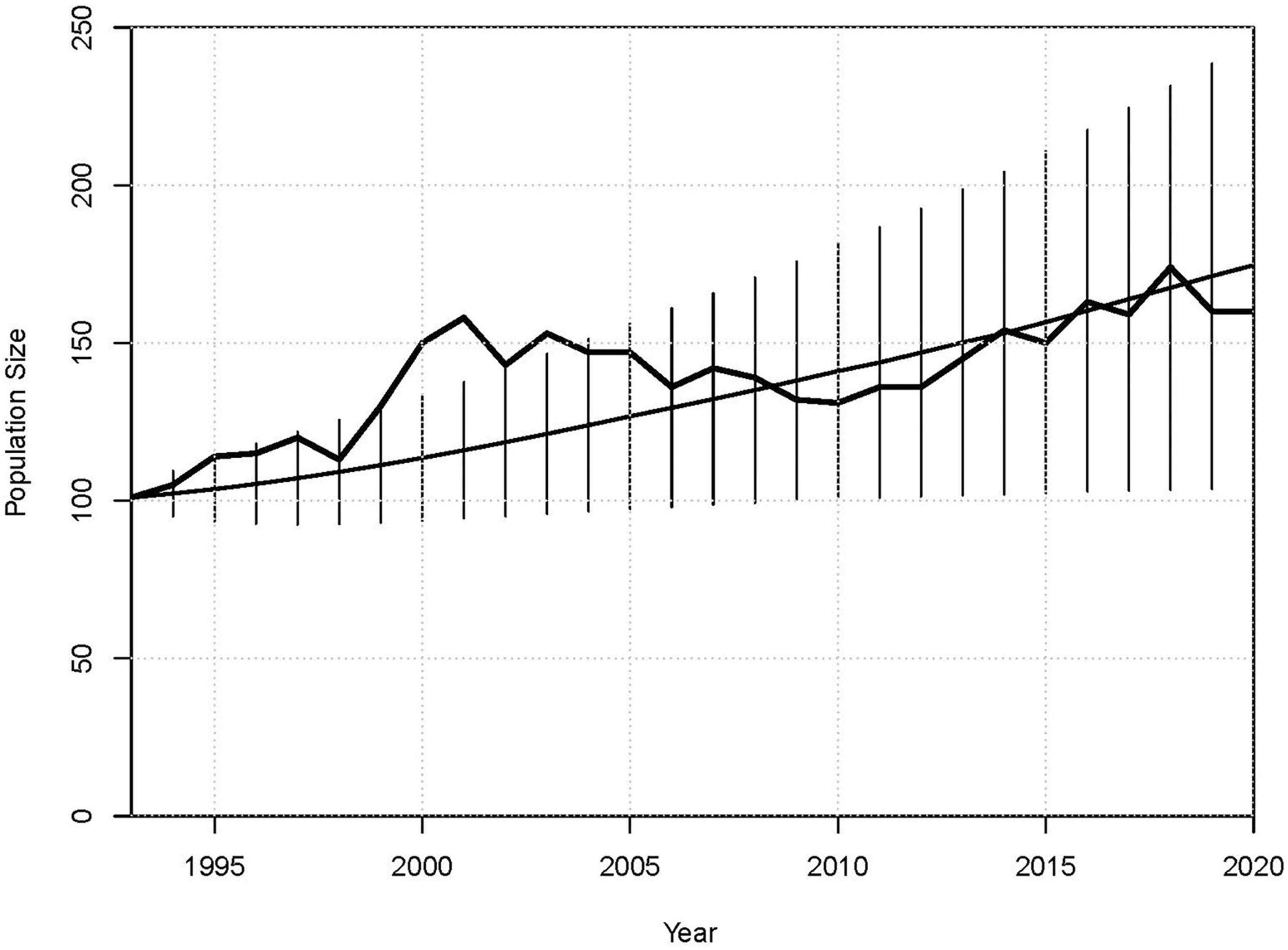
Figure 2. Mean projected population sizes from 1993 to 2020, with error bars showing the approximate 95% of the distribution of N across 10,000 iterations, and observed size of the Sarasota Bay population (heavier line) as of the start of each year.

The sex and age structure resulting from the simulations matched closely that of the current (January 2020) population. The predicted sex and age structure at the end of the Validation scenario (54.8% females and 25.8% juveniles [through age 5 years]) was similar to the 2020 observed structure (51.6% female, 25.0% juveniles). The long-term stable age structure of the Baseline scenario (54.1% female, 25.4% juveniles) also closely matched these numbers. The accuracy of the predicted sex and age structure indicates that the proportional mortality rates were accurately represented in the model.

Baseline Projections

When the simulation treated all losses as deaths and included observed immigration (appearances of non-infant dolphins not previously observed in the population), the model projects a long-term mean population growth of r = 0.021 (Table 5). This is marginally faster population growth than the observed trend from 1993 to 2020 and the Validation scenario. As with the Validation scenario, the annual fluctuations in population size, SD(r) = 0.031, in the Baseline projection are less than observed from 1993 to 2020. Samples of the projections from 25 iterations of the Baseline are shown in Figure 3. The population is projected to reach the carrying capacity of K = 200 imposed in the model in about 10 years, and thereafter to remain relatively stable (final mean N = 197, SD(N) = 5.9, 95% CI = 186 to 209).

TABLE 5

Table 5. Results for scenarios projecting population growth for the Sarasota Bay population of bottlenose dolphins.

FIGURE 3

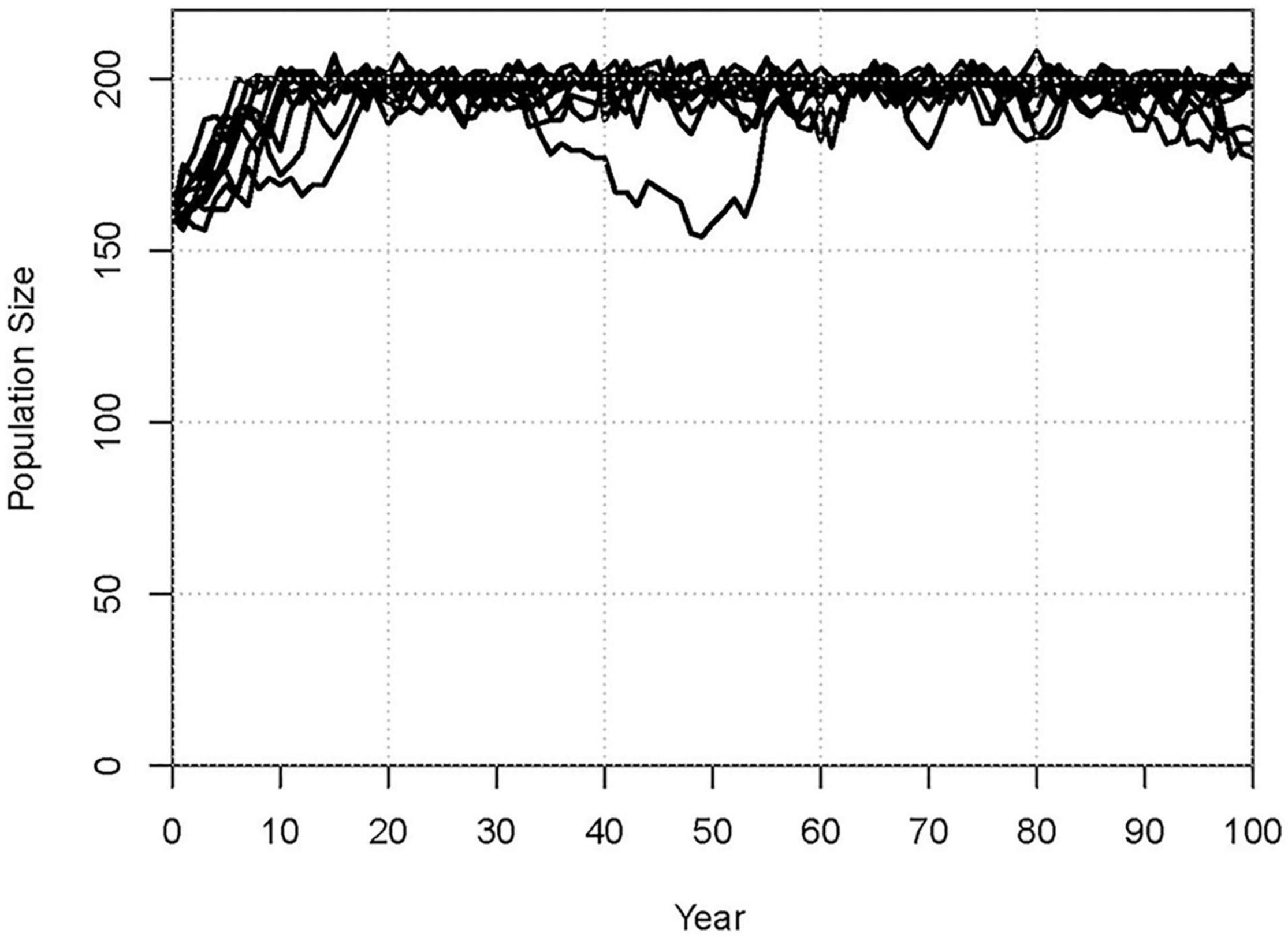
Figure 3. Population trajectories for a sample of 10 iterations of the Baseline scenario, illustrating the typical variation among iterations and across years of the simulation.

Alternative Estimates of Mortality Rates

Table 5 shows also the results for scenarios if the population were closed to immigration and mortality rates were set to values that represent possible values for actual mortality – not including losses due to emigration. When mortality was set to the rates estimated from the reported 0.33 recovered carcasses (confirmed deaths) per actual deaths (Estimated Mortality scenario), the population growth (r = 0.023) closely matched that of the Baseline scenario that included emigration (via treating all losses as deaths) and immigration. The minimum possible mortality, including only documented deaths, resulted in a population growth of r = 0.042, nearly twice the projection when estimates of unobserved deaths are included. The maximum possible mortality, considering all losses as deaths (assuming no emigration), resulted in a still positive r = 0.016 growth rate.

Tolerance of Additional Mortality

Scenarios that set survival of each age class to be 95% up to 100% of estimated values projected that mean population growth would be reduced to r = 0.017 with 0.5% reduction in survival, to r = 0.012 with 1% reduction in survival, r = 0.000 with a 2.5% reduction, and r = −0.013 with a 5% reduction in survival. The effect of decreasing survival on population growth is illustrated in Figure 4.

FIGURE 4

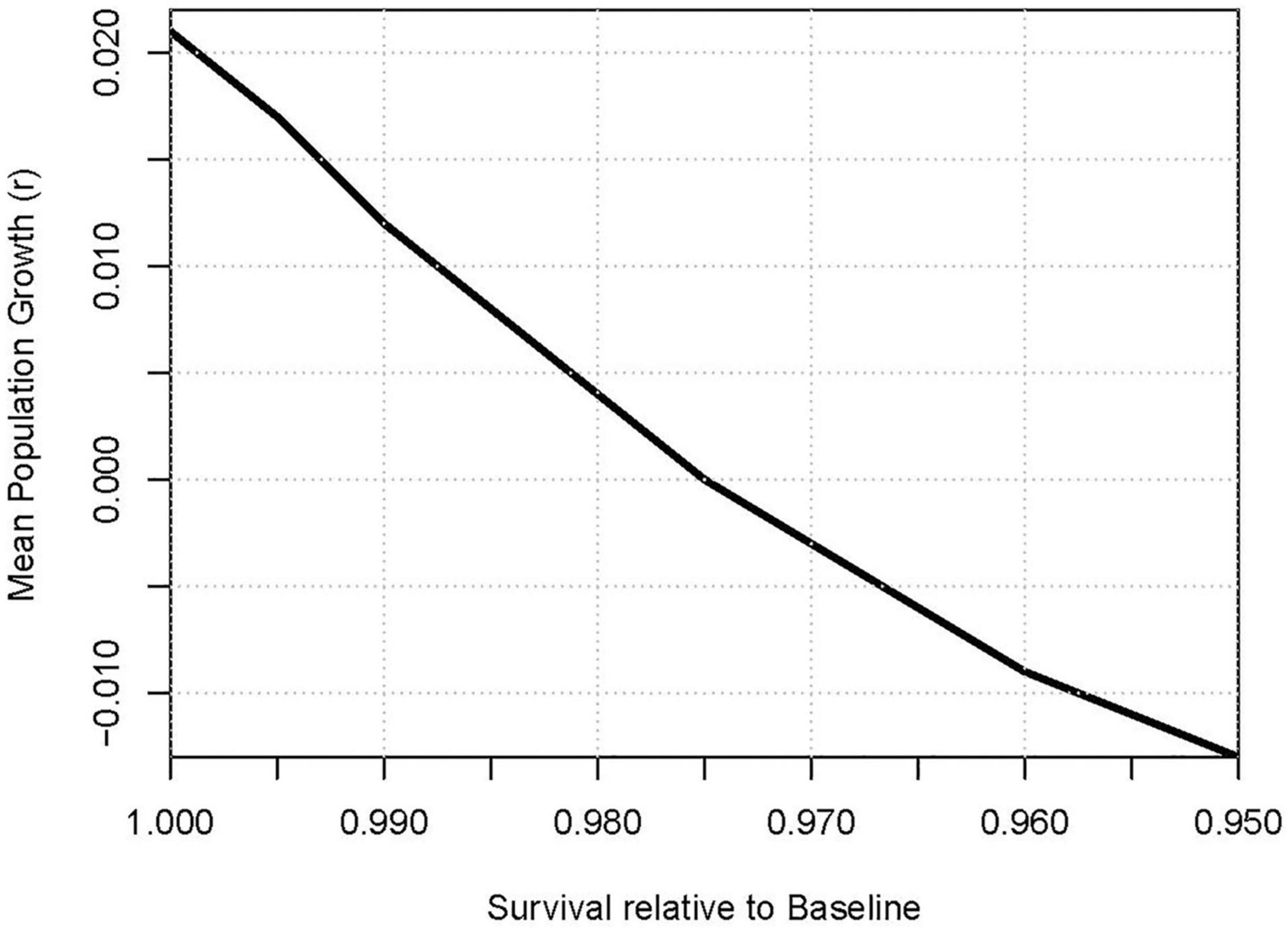
Figure 4. Effect of additional mortality (scaled as proportional reduction of survival) on projected mean population growth.

Red Tides

When the 2 years with higher mortality associated with severe red tide events (2006 and 2019) are omitted from the data used for calculating mortality rates, the estimated calf mortality decreased from 24.1% to 22.9%, and juvenile mortality decreased from 8.1% to 7.3%, causing the projected population growth to be elevated to r = 0.023 (SD = 0.029), compared to r = 0.021 (SD = 0.031) for the Baseline scenario (Table 5). When the mortality rates for those 2 years were duplicated, calf mortality increased to 25.1%, juvenile mortality increased to 8.7%, and the growth rate was slightly lower than Baseline, with r = 0.019 (SD = 0.032).

Minimum Viable Population

Tests of viability of small, closed populations projected an extinction probability over 100 years of 44% at the smallest size (K = 10), but extinction dropping to just 4% for K = 20, and less than 1% when K ≥ 30 (Figure 5A). The greater demographic stochasticity of the small size populations depressed growth to r = 0.014 for K = 10, r = 0.019 for K = 20, and growth approached a plateau of the r = 0.023 level observed in the Estimated mortality model for Sarasota (where K = 200) when K exceeded 60 (Figure 5B). These results, however, were generated by a model that excludes any negative impact of accumulated inbreeding. Although the severity of inbreeding depression in closed populations of dolphins is not known, populations of K = 10 (if they persisted) retained over the 100 years (5 generations) only 53% of initial gene diversity, which is approximately the expectation after a generation of selfing. With K = 20, 74% of gene diversity was retained (approximately the expectation after a generation of full-sib mating), and not until K > 50 was a closed population projected to retain 90% of its initial gene diversity (Figure 5C).

FIGURE 5

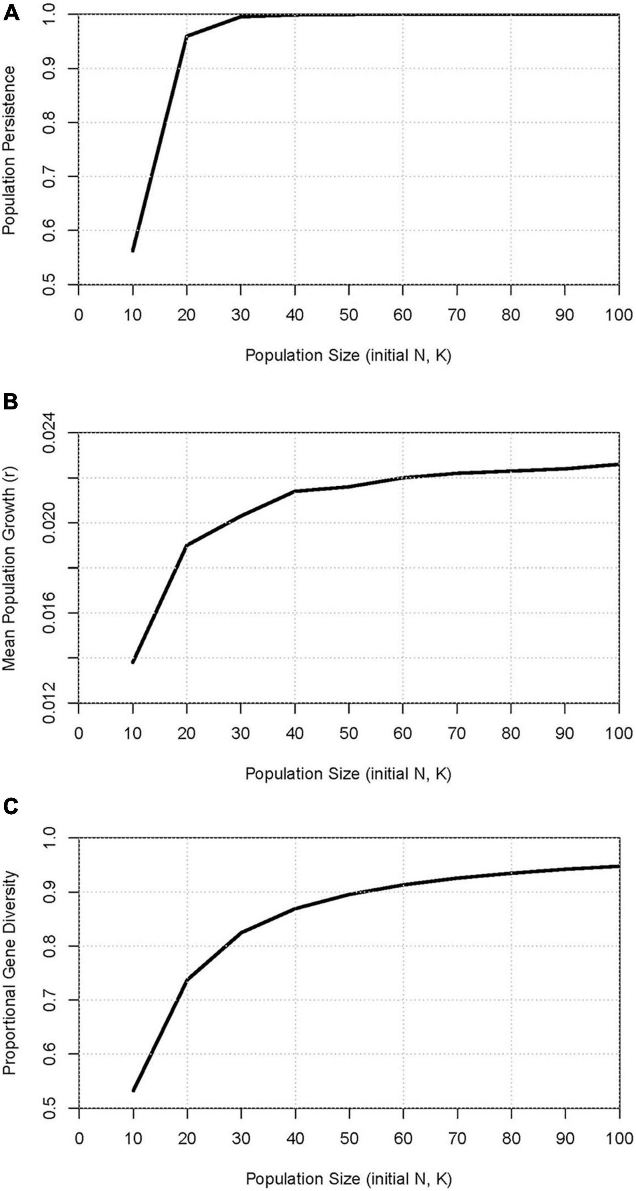
Figure 5. Measures of viability over 100 years in extant simulated populations that are closed to immigration with starting size (N) and carrying capacity (K) varied from 10 to 100: (A) probability of population persistence, (B) projected mean population size, and (C) proportion of gene diversity retained.

Resilience to Catastrophes

Figure 6 shows the projected recovery of the population following a catastrophe that caused the loss of 25%, 50%, or 75% of the dolphins. On average, it would take 11, 28, or 51 years, respectively, for the population to recover to its 2020 size, and about 30, 60, or nearly 100 years to approach the carrying capacity of N = 200.

FIGURE 6

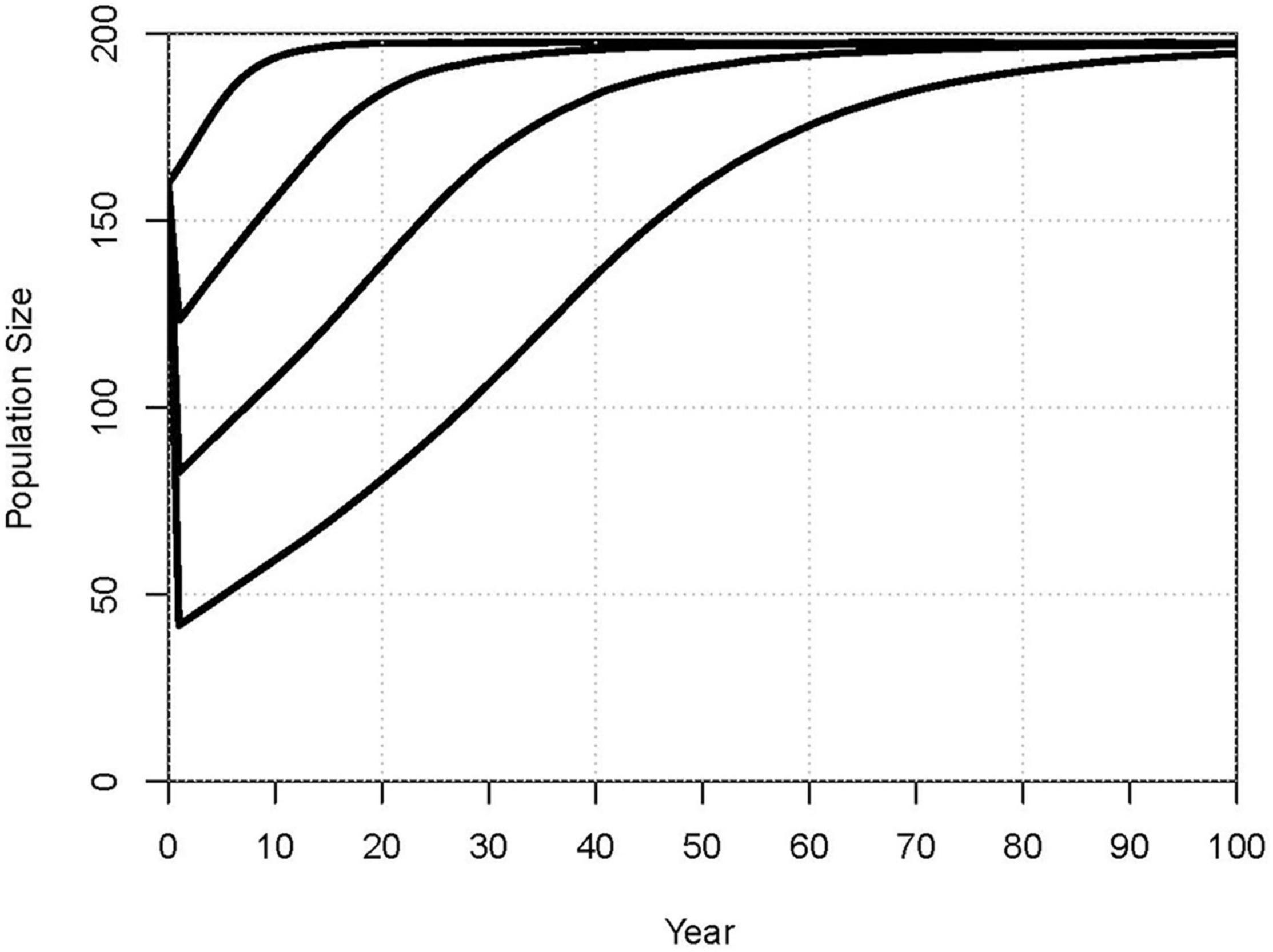
Figure 6. Projected mean rates of recovery after a catastrophe causes the loss of 0%, 25%, 50%, or 75% (lines top to bottom) of the dolphins.

Sensitivity Analysis

The comparative impacts of uncertainties in model parameters can be illustrated by “spider plots” that show the projected mean population growth for each level of the parameters that were varied. Figure 7 shows the mean r when each demographic rate was set to the estimated mean −2 SE, −1 SE, +1 SE, or +2 SE. The steepest line shows that the uncertainty in breeding rate of peak age (12 to 25 years) females had the largest impact on the projected population growth, with growth ranging from 1.2% to 3.1% per year across ± twice the SE (the approximate 95% confidence interval). Uncertainty in mortality of this age class has the next largest impact on results, with a range from 1.7% to 2.7% growth across the parameter uncertainty.

FIGURE 7

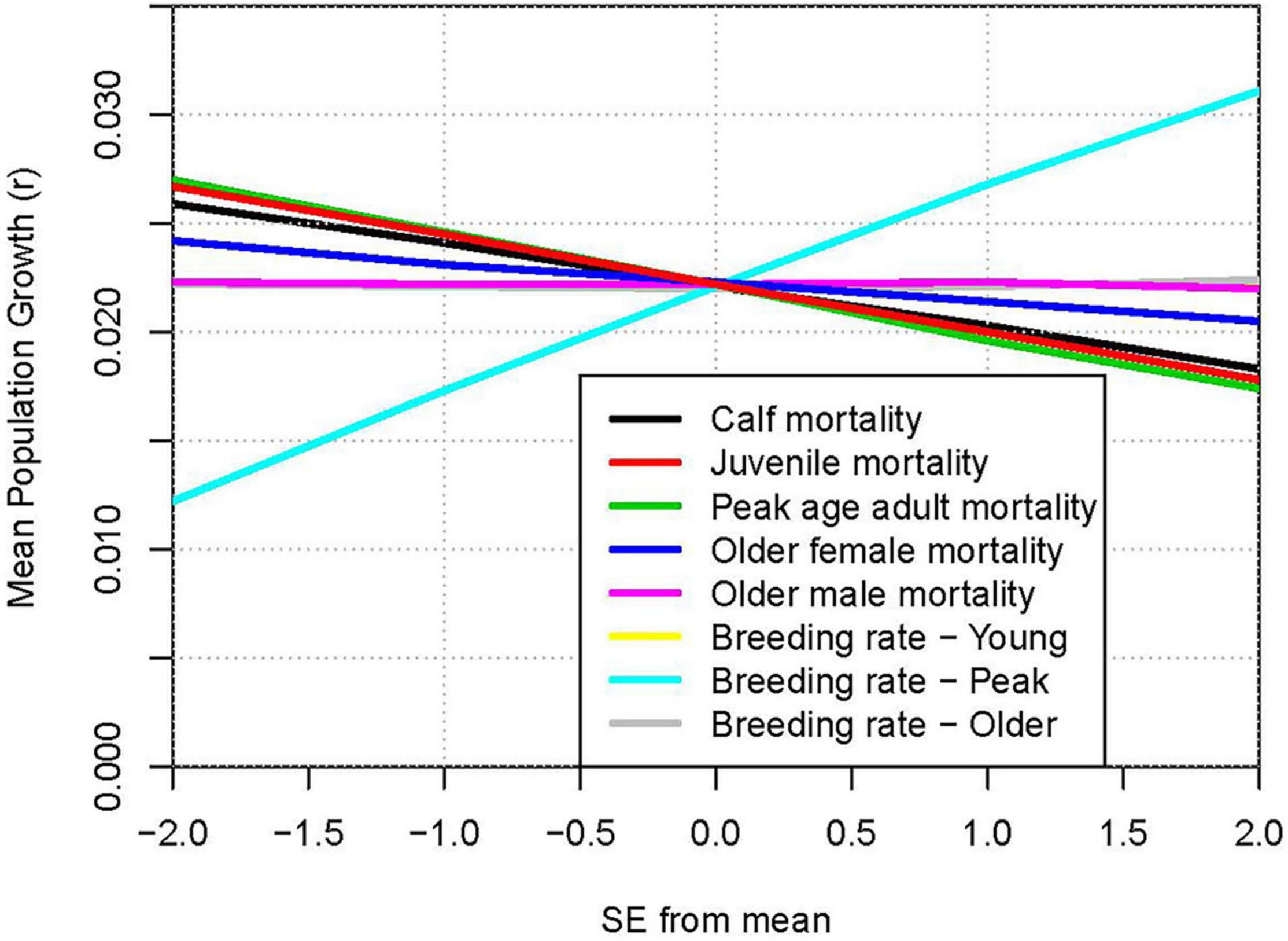
Figure 7. Relative impacts of uncertainty in parameter estimates: Population growth rate (r) when demographic rates are varied from −2 SE to +2 SE around the mean estimated values. Lines from top to bottom on right hand ends: Breeding rate – Peak (positive slope); three superimposed lines with slope ≈ 0: Older male mortality, Breeding rate – Young, Breeding rate – Older; lines with negative slopes: Older female mortality; Calf mortality; Juvenile mortality; Peak age adult mortality.

The variation among iterations (SD = 0.0070) in the mean population growth across all 100 years is necessarily much smaller than the variation (SD = 0.031) in annual population changes (r each year), because the long-term r is averaged over 100 years, because the variation in growth is less in later years of the simulation than in early years affected by current age structure, and because temporal fluctuations (due to environmental variation and demographic stochasticity) mostly average out over time. Of the variation in long-term mean growth, a portion with SD = 0.0062 is due to the uncertainties in demographic rates, with a residual of SD = 0.0032 due to environmental variation and demographic stochasticity. Table 6 shows the partitioning of variance in projected population growth (r) resulting from the models in which uncertain parameter values were sampled from distributions. The proportion of variation in the mean growth (averaged over the years of the simulation) due to the uncertainties (SEs) in each estimated parameter (Table 6, first two columns of values) showed that uncertainty in the breeding rate for peak reproductive years (12 to 25 years) accounted for nearly half of the variation across iterations. The uncertainties in the slopes of the increase in breeding from age 6 to 11 years and the decrease from age 26 to 48 years had negligible impact on population performance. Uncertainties in the mortality rates for calves, juveniles, and adults up through 25 years accounted for another 30% of the variation. Uncertainty in mortality of older (>25 years) males and females had very little effect of population growth, even though the SEs of those estimates were larger than the SEs for younger age classes (Table 3), because the dolphins that survive to older ages have declining reproductive rates, and therefore contribute much less to population growth.

TABLE 6

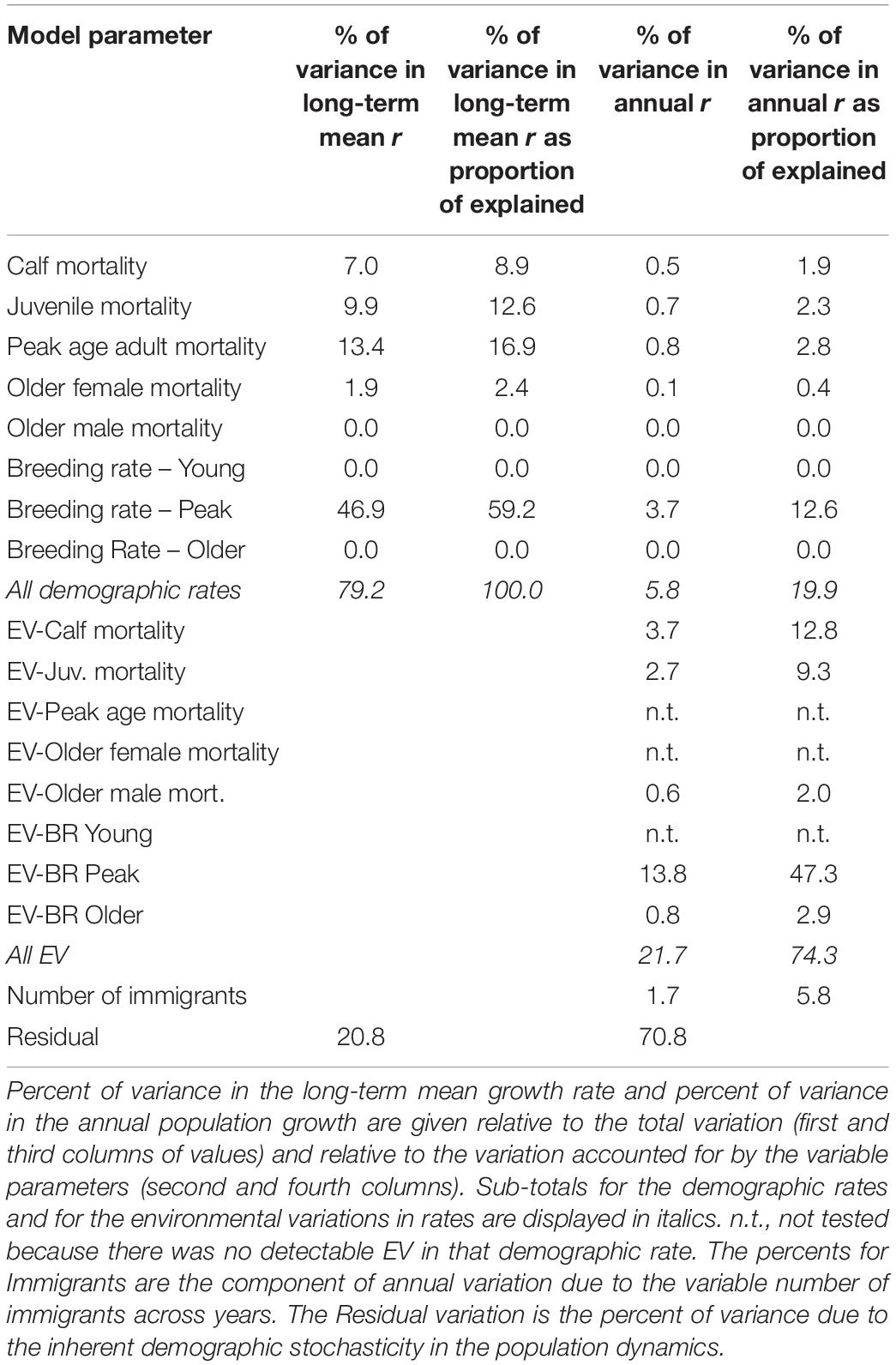
Table 6. Partitioning of variance in projected population growth (r).

Figure 8 shows the ranges of population growth that result from tests across the variability (EV) observed for demographic rates over the 27 years of censuses. When the mean rate for a demographic parameter was fixed at the mean −2 EV, −1 EV, +1 EV, or +2 EV, the natural variability in peak breeding rate had the largest impact on annual population growth. The impacts of annual variation in calf and juvenile mortality were next most important determinants of annual growth. No EV was detected for mortality of young adult and older adult females (Table 3), and effects of those two EVs were not considered in the sensitivity tests. Therefore, even though breeder survival could have considerable impact on population growth, it does not appear to be sensitive to annual fluctuations in environmental conditions.

FIGURE 8

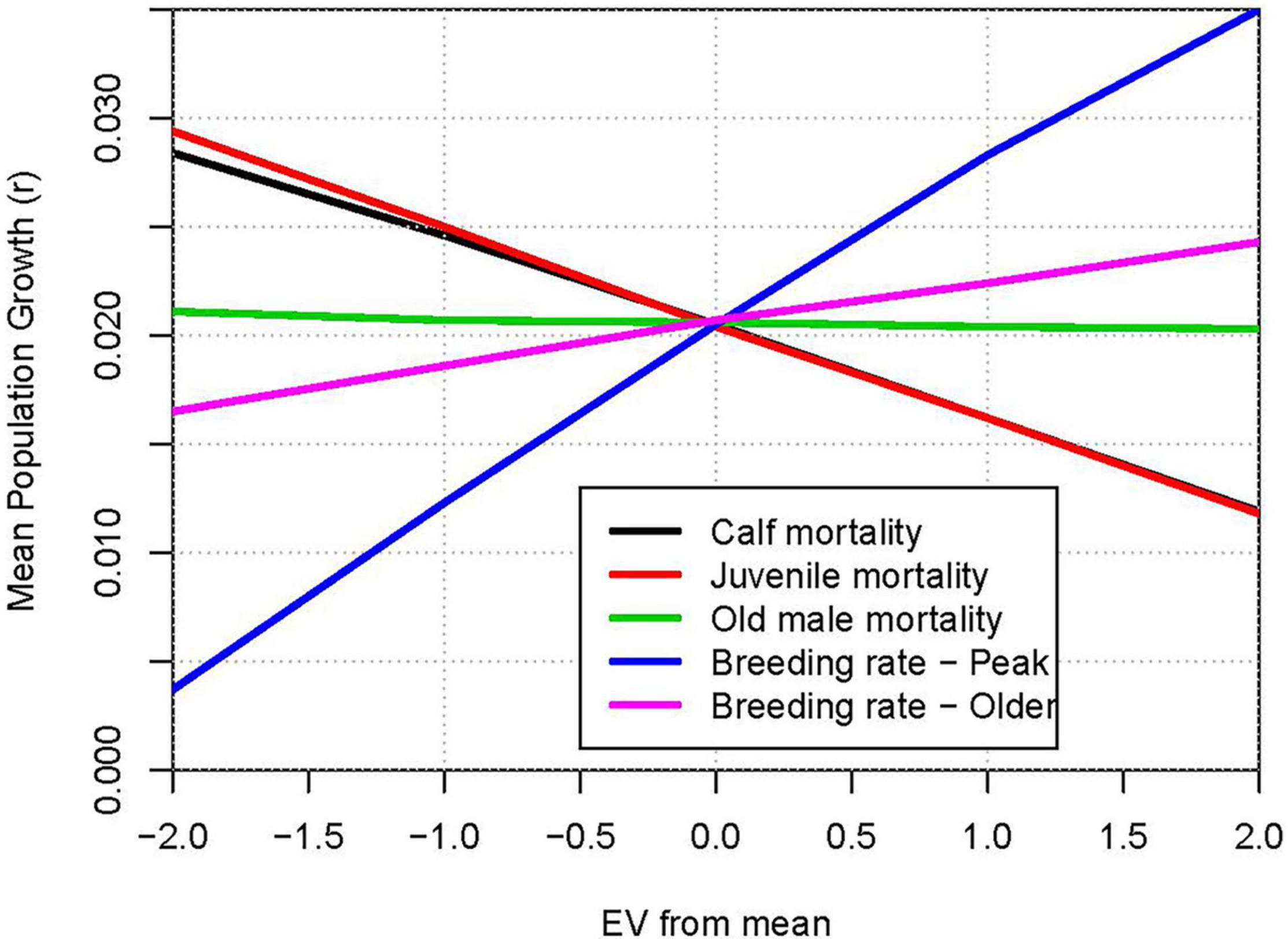
Figure 8. Relative impacts of environmental variation in demographic rates: Population growth rate (r) when demographic rates are varied from −2 EV to +2 EV around the mean estimated values. Lines from top to bottom on right hand ends: Breeding rate – Peak; Breeding rate – Older; Older male mortality (slope ≈ 0); Calf mortality; Juvenile mortality.

The partitioning of variance in annual population growth (last two columns of Table 6) considered the contribution of uncertainties in parameter estimates and also the contribution of the environmental variation in annual rates and the variation in the number of immigrants each year. The EVs in five demographic rates together contributed almost four-fold more to the annual fluctuations in population growth than did the combined contributions of sampling error (SEs) in the mean demographic rates. The variation in the number of immigrants added each year to the simulated population, sampled from a Poisson distribution, accounted for little (1.7%) of the variation in population size. The residual variation in annual population growth resulting from the demographic stochasticity in birth and death processes accounted for 71% of the variance in the simulation trajectories.

Discussion

Long-term monitoring of the Sarasota Bay dolphin community provides demographic information at a level of detail and precision rare in studies of cetaceans or any wild populations. Thus, the description of population demography for this population can serve as a standard for PVAs on small cetaceans. A PVA of the Sarasota Bay population of bottlenose dolphins was therefore undertaken with multiple purposes:

(1) Documenting the demographic rates in sufficient detail and accuracy to provide confidence in derived estimates of population growth;

(2) Presenting the natural variability in demographic rates and the uncertainties in mean rates due to the restrictions of sampling a specific population or social community for a moderate number of years;

(3) Exploring for which demographic rates the natural variability and measurement uncertainty has the largest effect on the confidence that can be placed on demographic projections;

(4) Estimating the minimum size of a closed population that could be considered demographically and genetically stable;

(5) Calculating the effect on population growth of several identified threats, including direct deaths due to human causes, and less direct impacts of environmental factors such as red tide events;

(6) Estimating the resilience of the population to any catastrophic declines, such as those that might result from a severe disease epidemic or catastrophic pollution event;

(7) Providing a well-documented baseline of demography and structure of a detailed PVA model for a coastal population of a small odontocete that can be used as a template or provisional default values to fill in data gaps for analyses of less well-studied cetaceans.

The Vortex PVA software has been used to assess population status, population growth and stability, relative threats, and management options for 100s of species⁴, including a number of marine mammals (e.g., dugong: Heinsohn et al., 2004; bottlenose dolphins: Thompson et al., 2000; Vermeulen and Bräger, 2015; Manlik et al., 2016; Blázquez et al., 2020; offshore dolphin species: Ashe et al., 2021; beluga whale: Williams et al., 2017; killer whale: Lacy et al., 2017; Murray et al., 2021; and Baltic harbor porpoise: Cervin et al., 2020). Vortex is an individual-based simulation that allows modeling of details of individual variation (e.g., variable ages of maturation and senescence), stochastic processes affecting small populations (e.g., demographic stochasticity, age structure perturbations, disrupted social structure, and local inbreeding), as well as the primary drivers of population trends of mean demographic rates. While not all of the options were used in this study, and factors should be omitted from population models when they are not of concern or thought to be consequential in the focal population, the options might be important for PVAs on other cetacean species. If all sources of stochasticity, dependencies on external variables, and non-linear interactions are removed from the model, the population projections generated by Vortex match those of standard matrix models of population growth (Caswell, 2001). The stochasticity in simulation models (and in real biological populations) will usually depress mean long-term population growth below that predicted from simpler matrix models (Lacy, 2000a).

In the past 27 years of consistent monitoring, the Sarasota Bay community of bottlenose dolphins has been growing at a mean rate of about 2% annually, but with considerable fluctuations across years (mean r = 0.019, SD(r) = 0.061, SE = 0.012, range r = −0.086 to 0.188). Consequently, even with 27 years of data, the precision with which we can predict the long-term mean population growth rate from the observed population trajectory is still limited, with a 95% CI (−0.006 to 0.044) that includes no population growth. This suggests that even for a long-lived mammal, with census data covering more years than is typically available for wildlife populations, fluctuations in population size make it difficult to estimate expected population growth by a simple extrapolation from recent census counts.

The census data used in our analyses should not be assumed to be a precise description of the resident population. The demographic rates were calculated from those identifiable animals observed to be present in the study area each year. These tallies omitted the small number of dolphins that were unidentifiable (estimated at <5% of total) and several that were long-term residents but had moved to adjacent waters for one or a few years⁵. However, unless the uncounted dolphins were a biased subset with respect to demographic rates, the estimates made from the animals observed in each year provide estimates of demographic rates with more accuracy and reliability than is available for almost any other free-ranging, wild population of vertebrates.

Among the advantages of using demographic models to project population growth from demographic rates, rather than simply extrapolating from recent observed census numbers, are: short-term fluctuations that result from perturbations of the age distribution will not carry forward and amplify projected trends in population growth; components and causes of variation in growth can be examined; effects of changes to specific demographic rates can be explored; and our understanding of the population dynamics can be tested by comparing results from mechanistic models to observed population trends and patterns.

The range of projections in the simulations encompassed the observed trends from 1993 to 2020, and the Validation scenario projected the same population growth rate as observed (r = 0.019), thereby validating that the model is a plausible representation of the population demography. The census trend with larger than projected size up through 2005, but with an apparent plateau subsequently (Figure 2), might indicate that the population has reached the ecological carrying capacity of the habitat. However, apparent trends could result from random fluctuations in population growth. In the decade since 2010, the observed population growth has been approximately parallel to the mean prediction of the simulations. With respect to validating the estimated demographic rates, it is notable that the variance in annual growth across years of the simulation was due much more to environmental variation and intrinsic demographic stochasticity than to uncertainty in estimates of mean demographic rates (Table 6). The mean demographic rates in this population have been sufficiently accurately estimated from the 27 years of surveys to provide reliable estimates of mean birth and death rates for modeling the population, while short-term fluctuations are expected due to the natural variability in the environment and demographic processes.

The Baseline population model that includes all additions (births plus immigrants) and losses (mortalities plus emigrants), projects a long-term mean population growth rate of r = 0.021, with variation among independent iterations of SD (100 years mean r) = 0.007, 95% CI = 0.007 to 0.034. Thus, although precise estimates of the mean of simulated trajectories can be made arbitrarily small by running a large number of repeats of the simulation [SE(mean r) = 0.00002 with 100,000 iterations], the intrinsic uncertainties of population processes, augmented by uncertainties in model parameter estimates, leaves us unable to predict accurately the fate of any specific population (whether the real one or one of the simulated trajectories).

The contributions of immigration and emigration to the observed population growth are hard to quantify, but a plausible assumption is that immigration and emigration are approximately off-setting on average, although much of the observed annual fluctuations in census numbers could be due to short-term net inflow or outflow of dolphins in response to local conditions. Without immigration, and with mortality estimated from the reported ratio of documented deaths relative to total deaths of 0.33 (the Estimated mortality scenario), we project intrinsic growth rate of r = 0.023, close to the projected growth when all immigration and emigration is included in the model. Even when all disappearances are assumed to be deaths and no immigration is included in the model (the Maximum mortality scenario), there was still a projected growth of r = 0.016. Thus, the Sarasota Bay population is not dependent on the few immigrants per year to be demographically stable, immigration and emigration contribute only moderately to the population dynamics, and it is appropriate to consider this community to be a biological population.

Several caveats about the projections should be recognized. First, a portion of the uncertainty in the estimated long-term mean growth was due to uncertainty in the demographic rates entered into the model. Thus, there remain improvements in precision of population growth projections that can be achieved by more data on demographic rates. Moreover, the census population size fluctuated more from year to year (SD(annual r) = 0.061) than occurred in the simulation (SD(annual r) = 0.035 in the Validation scenario). This suggests that there were causes of variation in population growth that were not captured in the model. Although almost all residents present in the population each year were tallied in the census data, some of the variation in observed population growth could have been caused by small sampling errors in the annual counts.

Further monitoring of the population size and demographic rates will be necessary to confirm the actual carrying capacity of the Sarasota Bay habitat. Although the population size has remained relatively flat over the last few years, suggesting that it might be near its carrying capacity, there is not yet evidence of density-dependent reductions in reproductive success. Moreover, the concept of carrying capacity simplistically assumes that the environment is stable over time, rather than increasing, decreasing, or being in a constant state of flux. Several recent changes likely affected carrying capacity and birth and death rates. A ban on commercial fishing with large gill nets in inshore Florida waters was imposed in 1995, and the increased population growth of dolphins from 1995 to 2000 could have resulted from increased prey availability and shifts in foraging patterns that might have improved reproduction (the 2 years with the highest birth rates were 1996 and 1999) or led to increased immigration into the local population. (There was a mean of 3.67 immigrants/year from 1995 through 2000, compared to a mean of 1.43 per year in the other 20 years.) Declines in the population in the few years after 2005 and in the most recent few years (apparently continuing into 2020) could have been consequences of the severe red tide events that occurred during 2005-2006 and 2018-2019 (Berens McCabe et al., 2021). The future environment might be very different from that of the recent past. The 100-year simulations represent the expected trajectories if conditions remain as they are, but PVA projections should not be assumed to be a prediction of the future.

An important contribution of PVA theory was the recognition that the stability and even long-term persistence of populations depends not just on mean demographic rates but also on the variation over time (“environmental variation,” EV) caused by fluctuations in the environment (Gilpin and Soulé, 1986). Moreover, the temporal variation in demographic performance determines the number of years of data that must be sampled in order to obtain reliable estimates of long-term means in demographic parameters. However, data from a number of years are needed in order to obtain estimates of EV, especially if there are occasional extreme years (i.e., catastrophes) that lie outside of the more typical annual variations. EV must be partitioned from the contribution of individual sampling error or demographic stochasticity to total annual variation in observed rates (Akçakaya, 2002; Lacy et al., 2020), and the sampling error can be a larger component than is EV when the numbers of observed demographic events are small, making accurate estimation of EV difficult. Consequently, many PVAs use crude estimates of EV based on few years of data, use total annual variation as an upper bounds estimate, use expert opinion based on the life history of the species, or use unvalidated rules of thumb such as assuming that EV will be approximately 20% of the mean for each demographic rate.

The long-term data on the Sarasota Bay population provides an opportunity to estimate EV for demographic modeling of a long-lived species. However, even with 27 years of data, the small number of births and deaths each year results in large binomial sampling variation around population probabilities of each type of demographic event, especially since separate estimates must be made for each age class that is found to have statistically different mean rates (e.g., calves, juveniles, young adults, peak age adults, and older adults). Thus, our calculated values for EV are still only approximate, albeit more accurate than is available for most other comparably long-lived animals. For adult mortality and young female fecundity, the expected binomial sampling error was as large or larger than the observed annual variation, indicating that we have no evidence for EV in those rates. For calf mortality, juvenile mortality, and breeding rates for females beyond 12 years of age, there was substantial EV (Tables 2, 3), and those variations in rates contributed substantially to the variation in projected growth rate from year to year (Table 6). This suggests that reproduction and survival of still-dependent offspring are life stages that are more susceptible to environmental conditions or specific threats than is survival of adult females.

Uncertainties in the future of wildlife populations – even in PVAs that use the most complete demographic data – arise from residual sampling error around demographic rate estimates made from finite (and often small) sample sizes, intrinsic demographic stochasticity, environmental variation in key habitat characteristics, changing local and global environments due to increasing human activity, and future management or conservation actions that impact the species. Consequently, exploration of the extent of our uncertainty and the component causes via sensitivity analysis is a necessary part of any PVA (McCarthy et al., 1995; Mills and Lindberg, 2002).

When demographic rates were varied across + 2 × SE, we found that uncertainty in the breeding rate had the largest effect on the estimated long-term population growth, with the mean annual population growth resulting from the lower and upper bounds tested (approximately the 95% confidence interval) ranging from about 1% to about 3% (Figure 7). This might indicate that research to improve the accuracy of estimates of breeding rate could help reduce considerably the uncertainty in projected population growth. However, given that virtually all surviving births in the population are being documented and most females are of known age, the only option to improve estimation of breeding rate might be to extend the data over more years or over a wider geographic area. If any calves are lost before being counted in the surveys, those neonatal deaths would not contribute to our estimates of breeding rate or calf mortality, nor to the population growth.

When demographic rates were varied across the observed environmental variation (±2 × SD), the demographic rate that had the greatest influence on population growth was again the breeding rate (Figure 8). Variation in calf mortality and juvenile mortality also had large effects. The importance of environmental variation in adult female mortality was not tested because the data do not show that there was any annual variation in adult female mortality beyond that expected due to binomial sampling. This contrasts with the generalization in population ecology that adult female mortality is expected to have the largest effect on population growth for species with low fecundity and long reproductive lifespans (Brault and Caswell, 1993; Caswell, 2001). However, that generalization derives from sensitivity analyses that vary each demographic parameter by equal proportions. Yet, if environmental variation affects fecundity and survival of early age classes to a much greater extent than it affects adult survival, then proportional sensitivity analyses do little to inform us about the demographic rates that drive differences in population growth across time or space (Mills et al., 1999; Mills and Lindberg, 2002; Mills, 2013). Similarly, the extent to which human activities can affect each life history stage needs to be considered when evaluating which stage should be the focus of management (Manlik et al., 2018). For the Southern Resident Killer Whales, Lacy et al. (2017) found that recovery actions needed to address the recently low reproductive success, because there was little scope for improving the already high adult survival.

It is notable that the largest contributor to the year-to-year variation in population growth in the model was the intrinsic demographic uncertainty resulting from the stochasticity of biological processes. This intrinsic stochasticity accounted for 71% of the variation in annual change in population size, in contrast to 22% of such variation being due to EVs in the probabilities of reproduction and mortality, less than 6% due to our imprecision of estimating mean demographic rates, and less than 2% due to the variation in numbers of immigrants. These results indicate that the natural variation in environmentally determined annual demographic rates and the probabilistic nature of individual demographic events are much greater factors limiting our ability to predict the population change in any given year than are the uncertainties in our estimates of mean demographic rates for this population. However, it should be reiterated that the model projected less annual fluctuation in population growth than has been observed, indicating that some sources of variation are underestimated or not accounted for in the model.

The use of population data from recent years to project future population trajectories implicitly assumes that the environment and the population’s responses to it (including any evolutionary adaptation) will remain unchanged. Thus, PVA baseline models should be seen as projections from current or other hypothesized conditions, rather than as predictions of the future. PVA modeling can be used to explore alternative possible futures through testing alternative demographic rates, predicted trends in rates, or functional relationships to environmental variables that can themselves be projected from other models (Keith et al., 2008; Aiello-Lammens et al., 2011; Lacy et al., 2013). The assumption of constancy of demography quantified from past observations will be increasingly challenged by the impacts of global warming and other aspects of climate change. PVA has been used to predict direct and indirect impacts of climate change on species viability (e.g., Brook et al., 2009; Lacy et al., 2016; Williams et al., 2017).

Increasing water temperatures occurring with global climate change might cause increased mortality to the dolphins in Sarasota Bay and the Gulf of Mexico due to increased metabolic demands (Costa et al., 2013), mobilization of organic pollutants that had been sequestered in blubber (Yordy et al., 2010), or increased exposure to pathogenic microorganisms (Buck et al., 2006). Although the extent of any such increases in direct and indirect threats due to climate change has not yet been quantified, the higher observed mortality in summer months suggests that future increases in water temperatures could have negative impacts (Wells, 2010). Other anthropogenic changes to the environment such as amount of accumulated toxins (see text footnote 3) and frequency of direct human interactions (Wells et al., 2008)⁶ can also potentially cause increased mortality in the future. Although we do not yet know if and to what extent mortality will change, we can test what increase in mortality would be tolerated before causing the dolphin population to go into decline. Not surprisingly, a 0.5% decrease in survival was projected to reduce population growth by about 0.5% (from r = 0.021 to r = 0.016), and a 2.5% reduction in survival results in a population with no growth. Thus, with an estimated K = 200, the loss of an additional one dolphin per year (0.5%) would cause significant harm. Conversely, a reduction in the number of deaths due to human interactions will yield comparable improvements in population growth (McHugh et al., 2021).

Similarly, PVA models can be valuable in informing estimates of the sustainable take under conditions of uncertainty. Incidental mortalities of marine mammals resulting from fisheries (bycatch) is regulated in the United States (NOAA, 2004) and elsewhere (Williams et al., 2008; Lonergan, 2011) based on the potential biological removal (PBR), calculated as PBR = N_min (R_max/2) F_R, in which N_min is a minumum population size estimate, R_max is the net reproductive rate (symbolized r in this paper, to distinguish it from the lifetime reproductive rate, which is often designated as R), and F_R is a recovery factor (Wade, 1998). Following Wade (1998), R_max is usually assumed to be 0.04 for cetaceans, unless there is population-specific demographic data to suggest otherwise. The use of a minimum estimate of N, division of R_max by 2, and application of the recovery factor are intended to make the calculation of sustainable losses conservative, thereby accommodating uncertainty in the values (Wade, 1998; Moore et al., 2009). However, Punt et al. (2018) noted that the efficacy of PBR approaches to protect vulnerable cetaceans from excess human-induced mortality was highly dependent on the accuracy of the default assumption of R_max = 0.04.

The Sarasota population is projected to grow at only half the rate often assumed in many PBR calculations for cetaceans. Prior PVAs on cetaceans have generally found r to be substantially less than 0.04 (e.g., Manlik et al., 2016; Lacy et al., 2017; Williams et al., 2017; Cervin et al., 2020; Ashe et al., 2021; Murray et al., 2021), but often those analyses were completed on populations already known to be in decline or at risk of decline. The Sarasota population is perhaps a better model for a population that is growing. Sarasota Bay is not a pristine habitat, as deaths occur due to human interactions (see text footnote 6), dolphins accumulate harmful levels of pollutants (Wells et al., 2005; Yordy et al., 2010; see text footnote 3), and red tide events might be exacerbated by both climate change and introduction of anthropogenic nutrients from the watershed (Van Dolah, 2000; Brand and Compton, 2007; Wells, 2010). However, no parts of the oceans are pristine and unaffected by anthropogenic activities, and the Sarasota Bay population of Tursiops might be considered to be typical of moderately affected coastal populations of marine mammals. Thus, the baseline maximum population growth for calculating PBR of cetaceans perhaps should be adjusted downward, as the standard formulation of PBR might be less conservative than has been assumed.

Among the threats that can affect dolphin survival and reproductive success are the harmful algal blooms such as red tide (Karenia brevis). The most severe red tide events in recent years (in 2005-2006, and 2018-2019) were associated with higher calf and juvenile mortality and population declines in 2006 and 2019. Model scenarios that either omitted or doubled the years with such increased mortality projected very small differences in population growth compared to the Baseline scenario. This indicates that the resistance of adult dolphins to the impacts of red tides (perhaps reflecting their behavioral flexibility and ability to adjust foraging patterns [Wells, 2010]) and the long reproductive lifespan of dolphins provides tolerance of the population to such events. The apparently increasing frequency of severe red tide events (Van Dolah, 2000; Brand and Compton, 2007) and the possibility of other or longer-term impacts on the population should be monitored to determine if the few simple red tide scenarios that we tested adequately represent the threats that the population might face in a changing environment.

Although the Sarasota Bay population of dolphins is not at risk of being so small and isolated that it would be demographically and genetically unstable if recent demographic trends continue, the detailed demographic model does provide an opportunity to evaluate the minimum viable size (MVP) of isolated coastal populations of dolphins. When we modeled a closed population with no immigration, populations of size N < 30 were found to be vulnerable to extinction, even in the absence of any inbreeding depression. The high survival and long reproductive lifespan of bottlenose dolphins affords demographic stability at much smaller sizes than are reported for MVPs of most mammalian species (Traill et al., 2007). However, N > 50 was necessary to keep genetic decay over 100 years (5 generations) to less than 90% of initial heterozygosity (a common criterion for genetic viability; Soulé et al., 1986), which is equivalent to accumulated inbreeding remaining below F = 0.10 (Lacy, 1995). This translates also to an effective population size of N_e = 23 for a population of size N = 50, giving an estimated N_e/N ratio of 0.46. This is likely an over-estimate, because the Vortex model assumes that all individuals of an age class are equally likely to reproduce and that mating is at random. Any greater than random variation in reproductive success would depress N_e/N and accelerate loss of genetic diversity.

While species with long reproductive lifespans and low fecundity can be demographically stable at small population sizes, and long generation times also reduce the rate of decay of genetic diversity in closed populations, those same life history characteristics can prevent the populations from recovering quickly from any catastrophic declines, such as those caused by disease outbreaks and spills of oil or other toxins. Our tests of resilience to such declines show, for example, that the Sarasota Bay dolphin population would not be expected to recover to its current size for 28 years after a 50% decline. Scott et al. (1988) reported a 53% reduction in abundance of a mid-Atlantic migratory coastal population of dolphins due to a morbillivirus outbreak, and they estimated a median recovery time of 32.5 years, or a median of 50.5 years if human-induced mortality due to fisheries continued at pre-outbreak levels.

A long reproductive lifespan can, however, buffer a population from short-term suppression of reproductive success, because females can skip a year of breeding and then resume or even compensate with increased breeding rate the following year. Thus, a 25% 1-year reduction in the breeding rate (affecting only the fewer than 30% of adult females that would have bred that year) can have much less consequence to the population than would a 25% reduction in survival in a catastrophe year. When catastrophic events reduce survival or breeding over a number of years, however, then the damage compounds and even long-lived species cannot cope by delaying breeding and responding with more reproduction a year or two later. Using a sex- and age-structured demographic model, Schwacke et al. (2017) projected that the dolphin population in Barataria Bay, Louisiana, would require 39 years to recover to its prior population size following the Deepwater Horizon oil spill in the Gulf of Mexico. The long recovery time resulted from reductions in survival that were estimated to last up to 10 years (with a 35% cumulative reduction observed over the first 3 years after the spill), compounded by a reduction of about 70% in reproductive success in each of the first 3 years and an estimated 17 years before reproduction would return fully to pre-spill levels.

The availability of data from 27 years of consistent monitoring of the individual dolphins resident in the Sarasota Bay population provided birth and death rates, allowed analysis of transition points in demographic rates as dolphins age, and provided the basis for a detailed demographic model that was validated against census data. The remaining uncertainties in population projections were partitioned into those due to sampling limitations, environmental fluctuations, and inherent stochasticity of demographic processes. Beyond the assessment of the Sarasota Bay population, the analyses can inform estimates of Minimum Viable Population (MVP) size for isolated, small populations and Potential Biological Removal (PBR) for directly or indirectly harvested populations. We used the PVA for some initial assessment of the resistance and resilience to threats affecting survival or breeding, and it can provide a basis for further investigations of the population-level impacts of causes of mortality that might be partitioned and quantified (e.g., McHugh et al., 2021) or of projected improvements in reproduction or survival resulting from management actions. Williams et al. (2020) noted that as the multiple effects of chronic ocean noise on cetaceans are measured, PVA can be used to quantify the population level impacts. Schwacke et al. (2017) described their demographic model as an important first step in determining the type and amount of restoration action needed to compensate for damage from the oil spill. Demographic impacts of singular or occasional events on the Sarasota population such as red tide, disease outbreaks, and the ban on large gill nets are difficult to quantify amid the multiple causes of population fluctuations, but long-term monitoring, data on other affected and non-affected populations, and mechanistic models of effects can provide estimates of impacts that could be explored through PVA. Such analyses are likely to be especially useful when integrated with other modeling approaches that have been applied to threat assessments for marine mammal populations, such as Pathways of Effects (PoE) (e.g., Murray et al., 2021), Population Consequences of Acoustic Disturbance (PCAD) (Williams et al., 2020), accumulation of Persistent Organic Pollutants (POPs) (Hall et al., 2006; Lacy et al., 2017), environmental changes driven by climate change (Williams et al., 2017), and metamodel linkages (Lacy et al., 2013) to examine predator-prey interactions with multi-species PVA (Lacy et al., 2016).

Data Availability Statement

The datasets presented in this study can be found in online repositories. The names of the repository/repositories and accession number(s) can be found below: The Vortex input files with all scenarios examined in this study are available in the zenodo.org repository at http://doi.org/10.5281/zenodo.5541834.

Ethics Statement

The animal study was reviewed and approved by the National Marine Fisheries Service Scientific Research Permits, with annual approvals by the Mote Marine Laboratory’s IACUC.

Author Contributions

RW provided and summarized the census and demographic data used for these analyses. RL constructed the population model and ran the scenarios. RL and RW interpreted the results and wrote the manuscript. RW, MS, KU, SH, JA, and AB were extensively involved in the collection and/or processing of survey and/or life history data, and/or oversaw data collection or processing operations. All authors contributed to the article and approved the submitted version.

Funding

Primary support for data collection or processing was provided by the Chicago Zoological Society, the Charles and Margery Barancik Foundation, the Batchelor Foundation, Earthwatch Institute, Disney Conservation Fund, Dolphin Quest, Inc., NOAA’s National Marine Fisheries Service, Don and Lee Hamilton, Edward McCormick Blair, Jr., Elizabeth Moore, and Rick and Nancy Moskovitz, and support for data analyses and writing by RW was provided by the Irvine Family.

Conflict of Interest

The authors declare that the research was conducted in the absence of any commercial or financial relationships that could be construed as a potential conflict of interest.

Publisher’s Note

All claims expressed in this article are solely those of the authors and do not necessarily represent those of their affiliated organizations, or those of the publisher, the editors and the reviewers. Any product that may be evaluated in this article, or claim that may be made by its manufacturer, is not guaranteed or endorsed by the publisher.

Acknowledgments

We gratefully acknowledge the assistance of the staff, students, and volunteers of the Chicago Zoological Society’s Sarasota Dolphin Research Program; in particular, current and former staff members Brian Balmer, Kim Bassos-Hull, Katie McHugh, and Stephanie Nowacek. We are grateful to Blair Irvine for initiating this research effort in 1970 and shepherding it through its initial years. We also appreciate the efforts of Larry Fulford for catch-and-release operations.

Footnotes

1. ^ Wells, R. S., Scott, M. D., Hohn, A. A., Sweeney, J. C., Townsend, F. I., Allen, J. B., et al. (in preparation). Life history, reproductive biology and demographic parameters for common bottlenose dolphins (Tursiops truncatus) in Sarasota Bay, FL. Front. Mar. Sci.
2. ^ Duffield, D. A., and Wells, R. S. (in preparation). Paternity patterns in a long-term resident bottlenose dolphin community. Front. Mar. Sci.
3. ^ Kucklick, J., Boggs, A., Huncik, K., Moors, A., Davis, E., Ylitalo, G., et al. (in review). Temporal tends of persistent organic pollutants in Sarasota Bay common bottlenose dolphins (Tursiops truncatus). Front. Mar. Sci.
4. ^ http://cpsg.org/document-repository
5. ^ Toms, C., Tyson Moore, R., Allen, J., McHugh, K., and Wells, R. S. (in preparation). Back to basics: a review of the residency construct and important considerations with respect to delphinid studies. Front. Mar. Sci.
6. ^ McHugh, K. A., Allen, J. B., Barleycorn, A. A., Bassos-Hull, K., Berens, McCabe, E., et al. (in preparation). Long-term human interaction trends within a multi-generational resident bottlenose dolphin community in Sarasota Bay, Florida. Front. Mar. Sci.

References

Aiello-Lammens, M., Chu-Agor, M. L., Convertino, M., Fischer, R. A., Linkov, I., and Akçakaya, H. R. (2011). The impact of sea-level rise on snowy plovers in Florida: integrating geomorphological, habitat, and metapopulation models. Glob. Change Biol. 17, 644–654.

Google Scholar

Akçakaya, H. R. (2002). Estimating the variance of survival rates and fecundities. Anim. Conserv. 5, 333–336. doi: 10.1017/s1367943002004092

CrossRef Full Text | Google Scholar

Ashe, E., Williams, R., Clark, C., Erbe, C., Gerber, L. R., Hall, A. J., et al. (2021). Minding the data-gap trap: exploring dynamics of abundant dolphin populations under uncertainty. Front. Mar. Sci. 8:606932. doi: 10.3389/fmars.2021.606932

CrossRef Full Text | Google Scholar

Beissinger, S. R. (2002). “Population viability analysis: past, present, future,” in Population Viability Analysis, eds S. R. Beissinger and D. R. McCullough (Chicago, IL: University of Chicago Press), 5–17.

Google Scholar

Beissinger, S. R., and McCullough, D. R. (eds) (2002). Population Viability Analysis. Chicago, IL: Chicago University Press.

Google Scholar

Berens McCabe, E. J., Wells, R. S., Toms, C. N., Barleycorn, A. A., Wilkinson, K. A., and Palubok, V. I. (2021). Effects of multiple Karenia brevis red tide blooms on a common bottlenose dolphin (Tursiops truncatus) prey fish assemblage: patterns of resistance and resilience in Sarasota Bay, Florida. Front. Mar. Sci. 8:711114. doi: 10.3389/fmars.2021.71114

CrossRef Full Text | Google Scholar

Blázquez, M., Baker, I., O’Brien, J. M., and Barrow, S. D. (2020). Population viability analysis and comparison of two monitoring strategies for bottlenose dolphins (Tursiops truncatus) in the Shannon Estuary, Ireland, to inform management. Aquat. Mamm. 46, 307–325. doi: 10.1578/am.46.3.2020.307

CrossRef Full Text | Google Scholar

Brand, L. E., and Compton, A. (2007). Long-term increase in Karenia brevis abundance along the southwest Florida coast. Harmful Algae 6, 232–252. doi: 10.1016/j.hal.2006.08.005

PubMed Abstract | CrossRef Full Text | Google Scholar

Brault, S., and Caswell, H. (1993). Pod-specific demography of killer whales (Orcinus orca). Ecology 74, 1444–1454. doi: 10.2307/1940073

CrossRef Full Text | Google Scholar

Brook, B. W., Akçakaya, H. R., Keith, D. A., Mace, G. M., Pearson, R. G., and Araujo, M. B. (2009). Integrating bioclimate with population models to improve forecasts of species extinctions under climate change. Biol. Lett. 5, 723–725. doi: 10.1098/rsbl.2009.0480

PubMed Abstract | CrossRef Full Text | Google Scholar

Buck, J. D., Wells, R. S., Rhinehart, H. L., and Hansen, L. J. (2006). Aerobic microorganisms associated with free-ranging bottlenose dolphins in coastal Gulf of Mexico and Atlantic Ocean waters. J. Wildl. Dis. 42, 536–544. doi: 10.7589/0090-3558-42.3.536

PubMed Abstract | CrossRef Full Text | Google Scholar

Caswell, H. (2001). Matrix Population Models, 2nd Edn. Sunderland, MA: Sinauer.

Google Scholar

Caswell, H., Brault, S., Read, A., and Smith, T. (1998). Harbor porpoise and fisheries: an uncertainty analysis of incidental mortality. Ecol. Appl. 8, 1226–1238.

Google Scholar

Cervin, L., Harkonen, T., and Harding, K. C. (2020). Multiple stressors and data deficient populations; a comparative life-history approach sheds new light on the extinction risk of the highly vulnerable Baltic harbour porpoises (Phocoena phocoena). Environ. Int. 144:106076. doi: 10.1016/j.envint.2020.106076

PubMed Abstract | CrossRef Full Text | Google Scholar

Costa, D. P., Worthy, G. A., Wells, R. S., Read, A. J., Waples, D., and Scott, M. D. (2013). “Patterns of seasonal metabolic rate variation for bottlenose dolphins in Sarasota Bay, Florida,” in Proceedings of the 20th Biennial Conference on the Biology of Marine Mammals, 9-13 December, Dunedin.

Google Scholar

Duffield, D. A., and Wells, R. S. (2002). “The molecular profile of a resident community of bottlenose dolphins, Tursiops truncatus,” in Molecular and Cell Biology of Marine Mammals, ed. C. J. Pfeiffer (Melbourne, FL: Krieger Publishing Company), 3–11.

Google Scholar

Ebenman, B., Law, R., and Borrvall, C. (2004). Community viability analysis: the response of ecological communities to species loss. Ecology 85, 2591–2600. doi: 10.1016/j.tree.2005.06.011

PubMed Abstract | CrossRef Full Text | Google Scholar

Gaston, K. J., and Fuller, R. A. (2008). Commonness, population depletion and conservation biology. Trends Ecol. Evol. 23, 14–19. doi: 10.1016/j.tree.2007.11.001

PubMed Abstract | CrossRef Full Text | Google Scholar

Gilpin, M. E., and Soulé, M. E. (1986). “Minimum viable populations: processes of extinction,” in Conservation Biology: The Science of Scarcity and Diversity, ed. M. E. Soulé (Sunderland, MA: Sinauer), 19–34.

Google Scholar

Hall, A. J., McConnell, B. J., Rowles, T. K., Aguilar, A., Borrell, A., Schwacke, L., et al. (2006). Individual-based model framework to assess population consequences of polychlorinated biphenyl exposure in bottlenose dolphins. Environ. Health Perspect. 114(Suppl. 1) 60–64. doi: 10.1289/ehp.8053

PubMed Abstract | CrossRef Full Text | Google Scholar

Heinsohn, R., Lacy, R. C., Lindenmayer, D. B., Marsh, H., Kwan, D., and Lawler, I. R. (2004). Unsustainable harvest of dugongs in Torres Strait and Cape York (Australia) waters: two case studies using population viability analysis. Anim. Conserv. 7, 417–425.

Google Scholar

JGI, TNC, CBSG, FZS, WCS, WD-MNRT, et al. (2011). Tanzania Chimpanzee Conservation Action Planning Workshop Report. Vienna, VA: Jane Goodall Institute.

Google Scholar

Keith, D. A., Akçakaya, H. R., Thuiller, W., Midgley, G. F., Pearson, R. G., Phillips, S. J., et al. (2008). Predicting extinction risks under climate change: coupling stochastic population models with dynamic bioclimatic habitat models. Biol. Lett. 4, 560–563. doi: 10.1098/rsbl.2008.0049

PubMed Abstract | CrossRef Full Text | Google Scholar

Lacy, R. C. (1995). Clarification of genetic terms and their use in the management of captive populations. Zoo Biol. 14, 565–577.

Google Scholar

Lacy, R. C. (2000a). Considering threats to the viability of small populations. Ecol. Bull. 48, 39–51.

Google Scholar

Lacy, R. C. (2000b). Structure of the VORTEX simulation model for population viability analysis. Ecol. Bull. 48, 191–203.

Google Scholar

Lacy, R. C. (2019). Lessons from 30 years of population viability analysis of wildlife populations. Zoo Biol. 38, 67–77. doi: 10.1002/zoo.21468

PubMed Abstract | CrossRef Full Text | Google Scholar

Lacy, R. C., Kovacs, K. M., Lydersen, C., and Aars, J. (2016). “Case study 4. Exploring impacts of declining sea ice on polar bears and their ringed seal and bearded seal prey in the northern Barents Sea,” in IUCN SSC Guidelines for Assessing Species’ Vulnerability to Climate Change. Version 1.0, eds W. B. Foden and B. E. Young (Gland: IUCN Species Survival Commission), 77–81.

Google Scholar

Lacy, R. C., Miller, P. S., Nyhus, P. J., Pollak, J. P., Raboy, B. E., and Zeigler, S. (2013). Metamodels for transdisciplinary analysis of population dynamics. PLoS One 8:e84211. doi: 10.1371/journal.pone.0084211

PubMed Abstract | CrossRef Full Text | Google Scholar

Lacy, R. C., Miller, P. S., and Traylor-Holzer, K. (2020). Vortex 10 User’s Manual. 7 August 2020 Update. Apple Valley, MN: IUCN SSC Conservation Breeding Specialist Group, and Chicago Zoological Society.

Google Scholar

Lacy, R. C., and Pollak, J. P. (2020). VORTEX: A Stochastic Simulation of the Extinction Process. Version 10.5.0. Brookfield, IL: Chicago Zoological Society.

Google Scholar

Lacy, R. C., Williams, R., Ashe, E., Balcomb, K. C. I. I. I., Brent, L. J. N., Clark, C. W., et al. (2017). Evaluating anthropogenic threats to endangered killer whales to inform effective recovery plans. Sci. Rep. 7:14119. doi: 10.1038/s41598-017-14471-0

PubMed Abstract | CrossRef Full Text | Google Scholar

Lonergan, M. (2011). Potential biological removal and other currently used management rules for marine mammal populations: a comparison. Mar. Policy 35, 584–589.

Google Scholar

Ludwig, D. (1996). Uncertainty and the assessment of extinction probabilities. Ecol. Appl. 6, 1067–1076. doi: 10.2307/2269591

CrossRef Full Text | Google Scholar

Manlik, O., Lacy, R. C., and Sherwin, W. B. (2018). Applicability and limitations of sensitivity analysis for wildlife management. J. Appl. Ecol. 55, 1430–1440. doi: 10.1111/1365-2664.13044

CrossRef Full Text | Google Scholar

Manlik, O., McDonald, J. A., Mann, J., Raudino, H. C., Bejder, L., Krützen, M., et al. (2016). The relative importance of reproduction and survival for the conservation of two dolphin populations. Ecol. Evol. 6, 3496–3512. doi: 10.1002/ece3.2130

PubMed Abstract | CrossRef Full Text | Google Scholar

McCarthy, M. A., Andelman, S. J., and Possingham, H. P. (2003). Reliability of relative predictions in population viability analysis. Conserv. Biol. 17, 982–989.

Google Scholar

McCarthy, M. A., Burgman, M. A., and Ferson, S. (1995). Sensitivity analysis for models of population viability. Biol. Conserv. 73, 93–100.

Google Scholar

McGowan, C. P., Runge, M. C., and Larson, M. A. (2011). Incorporating parametric uncertainty into population viability analysis models. Biol. Conserv. 144, 1400–1408. doi: 10.1111/cobi.12626

PubMed Abstract | CrossRef Full Text | Google Scholar

McHugh, K. A., Barleycorn, A. A., Allen, J. B., Bassos-Hull, K., Lovewell, G., Boyd, D., et al. (2021). Staying alive: long-term success of bottlenose dolphin interventions in southwest Florida. Front. Mar. Sci. 7:624729. doi: 10.3389/fmars.2020.624729

CrossRef Full Text | Google Scholar

Mills, L. S. (2013). Conservation of Wildlife Populations: Demography, Genetics, and Management, 2nd Edn. Oxford: Wiley-Blackwell.

Google Scholar

Mills, L. S., Doak, D. F., and Wisdom, M. J. (1999). Reliability of conservation actions based on elasticity analysis of matrix models. Conserv. Biol. 13, 815–829. doi: 10.1046/j.1523-1739.1999.98232.x

CrossRef Full Text | Google Scholar

Mills, L. S., and Lindberg, M. S. (2002). “Sensitivity analysis to evaluate the consequences of conservation actions,” in Population Viability Analysis, eds S. R. Beissinger and D. R. McCullough (Chicago, IL: University of Chicago Press), 338–366.

Google Scholar

Moore, J. E., Wallace, B. P., Lewison, R. L., Zydelis, R., Cox, T. M., and Crowder, L. B. (2009). A review of marine mammal, sea turtle and seabird bycatch in USA fisheries and the role of policy in shaping management. Mar. Policy 33, 435–451. doi: 10.1016/j.marpol.2008.09.003

CrossRef Full Text | Google Scholar

Morris, W. F., and Doak, D. F. (2002). Quantitative Conservation Biology. Theory and Practice of Population Viability Analysis. Sunderland, MA: Sinauer.

Google Scholar

Murray, C. C., Hannah, L., Doniol-Valcroze, T., Wright, B., Stredulinsky, E., Nelson, J. C., et al. (2021). A cumulative effects model for population trajectories of resident killer whales in the Northeast Pacific. Biol. Conserv. 257:109124. doi: 10.1016/j.biocon.2021.109124

CrossRef Full Text | Google Scholar

NOAA (2004). Authorization for Commercial Fisheries Under the Marine Mammal Protection Act of 1972; Zero Mortality Rate Goal, Vol. 69. Washington, DC: Federal Register.

Google Scholar

Prowse, T. A. A., Bradshaw, C. J. A., Delean, S., Cassey, P., Lacy, R. C., Wells, K., et al. (2016). An efficient protocol for the sensitivity analysis of complex ecological models. Ecosphere 7:e01238.

Google Scholar

Punt, A. E., Moreno, P., Brandon, J. R., and Matthews, M. A. (2018). Conserving and recovering vulnerable marine species: a comprehensive evaluation of the US approach for marine mammals. ICES J. Mar. Sci. 75, 1813–1831. doi: 10.1093/icesjms/fsy049

CrossRef Full Text | Google Scholar

Pusey, A. E., Pintea, L., Wilson, M. L., Kamenya, S., and Goodall, J. (2007). The contribution of long-term research at Gombe National Park to chimpanzee conservation. Conserv. Biol. 21, 623–634. doi: 10.1111/j.1523-1739.2007.00704.x

PubMed Abstract | CrossRef Full Text | Google Scholar

Ralls, K., Beissinger, S. R., and Cochrane, J. F. (2002). “Guidelines for using population viability analysis in endangered-species management,” in Population Viability Analysis, eds S. R. Beissinger and D. R. McCullough (Chicago, IL: University of Chicago Press), 521–550.

Google Scholar

Reed, J. M., Mills, L. S., Dunning, J. B. Jr., Menges, E. S., McKelvey, K. S., Frye, R., et al. (2002). Emerging issues in population viability analysis. Conserv. Biol. 16, 7–19.

Google Scholar

Saether, B., and Engen, S. (2002). “Including uncertainties in population viability analysis using population prediction intervals,” in Population Viability Analysis, eds S. R. Beissinger and D. R. McCullough (Chicago, IL: University of Chicago Press), 5–17. doi: 10.1111/j.1461-0248.2007.01105.x

PubMed Abstract | CrossRef Full Text | Google Scholar

Scheffers, B. R., De Meester, L., Bridge, T. C. L., Hoffmann, A. A., Pandolfi, J. M., Corlett, R. T., et al. (2016). The broad footprint of climate change from genes to biomes to people. Science 354:aaf7671. doi: 10.1126/science.aaf7671

PubMed Abstract | CrossRef Full Text | Google Scholar

Schwacke, L. H., Thomas, L., Wells, R. S., McFee, W. E., Hohn, A. A., Mullin, K. D., et al. (2017). Quantifying injury to common bottlenose dolphins from the Deepwater Horizon oil spill using an age-, sex- and class-structured population model. Endanger. Species Res. 33, 265–279. doi: 10.3354/esr00777

CrossRef Full Text | Google Scholar

Scott, G. P., Burn, D. M., and Hansen, L. J. (1988). “The dolphin die-off: long-term effects and recovery of the population,” in Proceedings of the OCEANS ‘88. A Partnership of Marine Interests, (Baltimore, MD), 819–823. doi: 10.1109/OCEANS.1988.794905

CrossRef Full Text | Google Scholar

Shaffer, M. L. (1981). Minimum viable population sizes for species conservation. Bioscience 31, 131–134.

Google Scholar

Simonis, J. L., Harrison, R. B., Long, S. T., Rabon, D. R. Jr., Waddell, W. T., and Faust, L. J. (2018). Managed movement increases metapopulation viability of the endangered red wolf. J. Wildl. Manag. 82, 573–582. doi: 10.1002/jwmg.21397

CrossRef Full Text | Google Scholar

Soulé, M., Gilpin, M., Conway, W., and Foose, T. (1986). The millennium ark: how long a voyage, how many staterooms, how many passengers? Zoo Biol. 5, 111–114.

Google Scholar

Thompson, P. M., Wilson, B., Grellier, K., and Hammond, P. S. (2000). Combining power analysis and population viability analysis to compare traditional and precautionary approaches to conservation of coast cetaceans. Conserv. Biol. 14, 1253–1263. doi: 10.1046/j.1523-1739.2000.00099-410.x

CrossRef Full Text | Google Scholar

Traill, L. W., Bradshaw, C. J. A., and Brook, B. W. (2007). Minimum viable population size: a meta-analysis of 50 years of published estimates. Biol. Conserv. 139, 159–166. doi: 10.1016/j.biocon.2007.06.011

CrossRef Full Text | Google Scholar

Traylor-Holzer, K. (2019). Population Viability Analysis (PVA) Report for the Species Meta-Population of Whooping Cranes (Grus americana). Apple Valley, MN: IUCN SSC Conservation Planning Specialist Group.

Google Scholar

Tyson, R. B., and Wells, R. S. (2016). Sarasota Bay/Little Sarasota Bay Bottlenose Dolphin Abundance Estimates: 2015. Prepared for National Marine Fisheries Service Northern Gulf of Mexico Bay, Sound and Estuary Bottlenose Dolphin Stock Blocks B20 and B35, Combined. Southeast Fisheries Science Center Reference Document PRBD-2016-02. Silver Spring, MD: NOAA, 22.

Google Scholar

Van Dolah, F. M. (2000). Marine algal toxins: origins, health effects, and their increased occurrence. Environ. Health Perspect. 108, 133–141. doi: 10.1289/ehp.00108s1133

PubMed Abstract | CrossRef Full Text | Google Scholar

Vermeulen, E., and Bräger, S. (2015). Demographics of the disappearing bottlenose dolphin in Argentina: a common species on is way out? PLoS One 10:e0119182. doi: 10.1371/journal.pone.0119182

PubMed Abstract | CrossRef Full Text | Google Scholar

Wade, P. R. (1998). Calculating the limits to the allowable human-caused mortality of cetaceans and pinnipeds. Mar. Mamm. Sci. 14, 1–37. doi: 10.1111/j.1748-7692.1998.tb00688.x

CrossRef Full Text | Google Scholar

Wells, R. S. (2010). Feeling the heat: potential climate change impacts on bottlenose dolphins. Whalewatcher J. Am. Cetacean Soc. 39, 12–17.

Google Scholar

Wells, R. S. (2014). “Social structure and life history of common bottlenose dolphins near Sarasota Bay, Florida: insights from four decades and five generations,” in Primates and Cetaceans: Field Research and Conservation of Complex Mammalian Societies: Primatology Monographs, eds J. Yamagiwa and L. Karczmarski (Tokyo: Springer), 149–172. doi: 10.1007/978-4-431-54523-1_8

CrossRef Full Text | Google Scholar

Wells, R. S. (2020). The Sarasota Dolphin Research Program in 2020: celebrating 50 years of research, conservation, and education. Aquat. Mamm. 25, 502–503. doi: 10.1578/AM.46.5.2020.502

CrossRef Full Text | Google Scholar

Wells, R. S., Allen, J. B., Hofmann, S., Bassos-Hull, K., Fauquier, D. A., Barros, N. B., et al. (2008). Consequences of injuries on survival and reproduction of common bottlenose dolphins (Tursiops truncatus) along the west coast of Florida. Mar. Mamm. Sci. 24, 774–794.

Google Scholar

Wells, R. S., Allen, J. B., Lovewell, G., Gorzelany, J., Delynn, R. E., Fauquier, D. A., et al. (2015). Carcass-recovery rates for resident bottlenose dolphins in Sarasota Bay, Florida. Mar. Mamm. Sci. 31, 355–368.

Google Scholar

Wells, R. S., Scott, M. D., and Irvine, A. B. (1987). “The social structure of free-ranging bottlenose dolphins,” in Current Mammalogy, Vol. 1, ed. H. Genoways (New York, NY: Plenum Press), 247–305. doi: 10.1007/978-1-4757-9909-5_7

CrossRef Full Text | Google Scholar

Wells, R. S., Tornero, V., Borrell, A., Aguilar, A., Rowles, T. K., Rhinehart, H. L., et al. (2005). Integrating life history and reproductive success data to examine potential relationships with organochlorine compounds for bottlenose dolphins (Tursiops truncatus) in Sarasota Bay, Florida. Sci. Total Environ. 349, 106–119. doi: 10.1016/j.scitotenv.2005.01.010

PubMed Abstract | CrossRef Full Text | Google Scholar

Williams, R., Cholewiak, D., Clark, C. W., Erbe, C., George, J. C., Lacy, R. C., et al. (2020). Chronic ocean noise and cetacean population dynamics. J. Cetacean Res. Manag. 21, 85–94.

Google Scholar

Williams, R., Hall, A., and Winship, A. (2008). Potential limits to anthropogenic mortality of small cetaceans in coastal waters of British Columbia. Can. J. Fish. Aquat. Sci. 65, 1867–1878. doi: 10.1139/f08-098

CrossRef Full Text | Google Scholar

Williams, R., Lacy, R. C., Ashe, E., Hall, A., Lehoux, C., Lesage, V., et al. (2017). Predicting Responses of St. Lawrence Beluga to Environmental Change and Anthropogenic Threats to Orient Effective Management Actions. Canadian Science Advisory Secretariat (CSAS) Research Document 2017/027. Ottawa, Ont: Fisheries and Oceans Canada, Canadian Science Advisory Secretariat, v+44.

Google Scholar

Yordy, J. E., Wells, R. S., Balmer, B. C., Schwacke, L. H., Rowles, T. K., and Kucklick, J. R. (2010). Partitioning of persistent organic pollutants between blubber and blood of wild bottlenose dolphins: implications for biomonitoring and health. Environ. Sci. Technol. 44, 4789–4795. doi: 10.1021/es1004158

PubMed Abstract | CrossRef Full Text | Google Scholar