Source Level of Antarctic Blue and Fin Whale Sounds Recorded on Sonobuoys Deployed in the Deep-Ocean Off Antarctica

Introduction

Antarctic blue whales (Balaenoptera musculus intermedia; ABWs) nearly became extinct due to 20th century industrial whaling (Rocha et al., 2015), and today they remain Critically Endangered (Cooke, 2018a). Over 700,000 Southern Ocean fin whales (Balaenoptera physalus quoyi) were killed during industrial whaling (Rocha et al., 2015), and their present day conservation status is Vulnerable (Cooke, 2018b). Despite 30 years of visual sightings surveys in the Southern Ocean following the moratorium on commercial whaling, there remain large knowledge gaps on the distribution and abundance of each species (Branch and Butterworth, 2001; Branch et al., 2007; Edwards et al., 2015). There is presently no accepted abundance or trend estimate for Southern Hemisphere fin whales, and the most recent estimate of population trend for Antarctic blue whales had large uncertainties regarding the rate of population increase, and furthermore is now over 20 years out of date (Branch, 2007).

Due to the low number of animals, the large area of the Southern Ocean that they potentially inhabit, and the expense of conducting scientific operations in the Antarctic, field biologists have sought newer, more efficient means of studying large whales than traditional line-transect surveys. Both ABWs and fin whales produce high-intensity, low-frequency vocalizations (Širović et al., 2004; Rankin et al., 2005) which can be detected over distances much larger than those over which whales can be seen from a ship (Širović et al., 2007; Samaran et al., 2010a; Miller et al., 2015). Thus, listening for these sounds via passive acoustic monitoring (PAM) offers an efficient means of detecting calling whales.

Contemporary projects conducted via the Southern Ocean Research Partnership of the International Whaling Commission (IWC-SORP; Bell, 2021) have adopted the use of PAM to more efficiently study ABWs and fin whales (Van Opzeeland et al., 2013; Peel et al., 2015). For example, the IWC-SORP Antarctic Blue Whale Project has adopted the use of PAM for real-time tracking of ABWs during voyages (Miller et al., 2015) to assist with obtaining a contemporary mark-recapture abundance estimate (Peel et al., 2015), as well as to understand foraging ecology (Miller E. J. et al., 2019) and movements on the feeding grounds (Andrews-Goff et al., 2013). Similarly, the recently established IWC-SORP Fin Whale Project aims to implement an integrated multi-disciplinary research program, including passive acoustics, to understand population structure, migratory behaviour, current population numbers, and feeding ecology of Southern Hemisphere fin whales (Herr, 2021). Furthermore, the IWC-SORP Acoustic Trends Project aims to investigate trends in both ABW and fin whale sounds to provide information on long-term trends in distribution, occupancy, and hopefully abundance, using data primarily from long-term, autonomous, moored recorders (Van Opzeeland et al., 2013).

A key knowledge gap that limits the utility of PAM of these species is limited knowledge of the source level and natural variation of ABW and fin whale vocalizations. The source level, SL, of a sound is defined as the equivalent power of the sound at 1 m from the source (ISO, 2017). SL, alongside noise level and reception/detection threshold, is a major factor in determining the area over which sounds can be detected. In addition to helping determine detection range of PAM systems, SL is also important in estimating the communication space of different call types, as well as the potential reduction of communication space that may arise from man-made noise (Payne and Webb, 1971; Clark et al., 2009).

Antarctic blue whales are known to produce two types of sounds: stereotyped, repeated, predominately tonal calls often referred to as song; and frequency-modulated (FM) downswept calls known as D-calls (Rankin et al., 2005). Fin whales in the Southern Ocean are also known to produce distinctive stereotyped song in the form of regularly repeated 20 Hz pulses (Širović et al., 2009; Buchan et al., 2019) as well as FM downswept calls, hereafter referred to as 40 Hz calls (Širović et al., 2006, 2013; Gedamke and Robinson, 2010; Miller et al., 2021a). For both ABWs and Southern Ocean fin whales, knowledge of source level is limited to only song calls, and this knowledge comes from a small number of calls, produced by an even smaller number of individuals (Širović et al., 2007; Samaran et al., 2010b; Bouffaut et al., 2021). While all populations of blue whales are known to produce D-calls, there are only three studies that present estimates of SL, and each of these for only a small number of calls all in the Northern Hemisphere (Thode et al., 2000; Berchok et al., 2006; Akamatsu et al., 2014). There are limited data on the SL of fin whale song from the Northern Hemisphere (Charif et al., 2002; Weirathmueller et al., 2013; Wang et al., 2016; Miksis-Olds et al., 2019). Recently Wiggins and Hildebrand (2020) presented the first SL estimates for fin whale 40 Hz calls, again from two animals in the Northern Hemisphere. There are no known estimates of SL of the D-calls produced by ABWs, nor the 40 Hz downswept calls of Southern Ocean fin whales.

Here we add to these studies on source levels of ABWs and fin whales using results from a passive acoustic survey conducted from the RV Investigator during the 2019 voyage: Euphausiids and Nutrient Recycling In Cetacean Hotspots (ENRICH) (Miller B. S. et al., 2019). On this voyage, pairs and triplets of Directional Frequency Analysis and Recording (DIFAR) sonobuoys were used to detect and triangulate the location of ABW and fin whale calls. These detections, along with acoustic propagation modelling based on Conductivity-Temperature-Depth (CTD) data enabled us to estimate SL of 1915 calls.

Materials and Methods

Estimation of Source Level

To estimate SL we applied the sonar equation for an omnidirectional source and receiver with no processing gain (Urick, 1983; Lurton, 2010) such that:

$SL=RL+TL$

here RL is the received sound pressure level of the sound measured at the sonobuoy, and TL is the transmission loss that occurs as the sound propagates through the environment from the whale to the sonobuoy. Our method for estimating SL was to make calibrated measurements of RL from calls originating at a known location, and to estimate TL for each detection of that call. In the sections below, we present a detailed description of the methods used to measure RL, triangulate call location, and estimate TL.

Call locations were obtained via triangulation of bearings from directional sonobuoys (detailed description below) which required detection of the same call on two or more different sonobuoys deployed concurrently. The mean SL for each triangulated call was obtained from all of the detections that comprised that triangulation. Thus, our sample size, n, for each call type was the number of calls, not the number of detections.

The detection of the same call at two or three hydrophones allows for the estimation of the variance due to various measurement errors separately from the variance due to whale depth and the natural variability in actual source level.

For a given call i detected at two hydrophones 1 and 2 we obtain two estimates of SL

$S{L}_{i,1}=S{L}_i+{\in }_1$

$S{L}_{i,2}=S{L}_i+{\in }_2$

where ∈ is an error term associated with the measurement error at each hydrophone (error in received level measurement plus error in transmission loss). To model the errors, we assume that ∈ are drawn from the same normal distribution for each measurement with mean 0 and standard deviation σ_∈. We then estimate the standard deviation of ∈ based on the n measurements as

${\widehat{\mathrm{\sigma }}}_{\in }=\sqrt{\frac{1}{n}\sum _{i=1}^{n}Var(S{L}_i)}$

Our estimate of ${\widehat{\mathrm{\sigma }}}_{\in }$ can then be compared to the standard deviation of SL across all calls, σ. If measurement error is much smaller (i.e., ${\widehat{\mathrm{\sigma }}}_{\in }\ll \mathrm{\sigma })$, then that would indicate that most of σ is due to natural variability. However, if ${\widehat{\mathrm{\sigma }}}_{\in }$ is of similar magnitude to σ, then most of the variability in our estimate of SL would appear to arise from measurement error and little can be learned about natural variability.

Acoustic System and Calibration

Listening stations during ENRICH survey were conducted by deploying SSQ-955 HIDAR sonobuoys in DIFAR mode to monitor for, and measure bearings to, vocalising whales while the ship was underway (Gedamke and Robinson, 2010; Miller et al., 2015). For most of the survey, listening stations were conducted with a single sonobuoy for one hour every 30–60 nmi in water depths greater than 200 m following a protocol nearly identical to Gedamke and Robinson (2010). However, some portions of the voyage were dedicated to whale studies or fine-scale krill surveys. During 205 h of these periods, arrays of two or three sonobuoys were deployed and recorded concurrently in order to triangulate calls following the protocol described by Miller et al. (2015).

The sonobuoy recording hardware, software, and sound-processing steps were identical to other recent voyages in 2013, 2015, 2018, and 2020 (Miller et al., 2015, 2016; Calderan et al., 2020; Jackson et al., 2020), and are also described in detail in the ENRICH voyage project report and passive acoustics report (Double, 2019; Miller B. S. et al., 2019). In brief, radio signals were received on an omnidirectional or Yagi directional antenna connected to a VHF receiver. Audio from the VHF receiver was digitized and recorded via a sound-board connected to a desktop computer.

Compass calibration followed procedures described in Miller et al. (2015, 2016). Calibrated sound pressure levels, for each detection and for measurements of noise levels, were obtained following the “intensity calibration” method described by Rankin et al. (2019). This frequency-domain method involved multiplying the frequency calibration-curves for the omnidirectional hydrophone given in the DIFAR specification (e.g., see Maranda, 2001; Greene et al., 2004), the radio receiver output level (nominally flat in frequency and 1.0 ± 0.2 V rms @ 75 kHz for a WinRadio G39-WSBe), and sound board (flat in frequency and 8.4 volts peak-peak limits for the analog instrument input with gain set to 20 dB).

Aural monitoring and visual inspection of spectrograms was conducted by an analyst (SC, BM, EM, AŠ, or KS) during the voyage. Monitoring was conducted in real-time, and the intensity scale of the spectrogram was adjusted by the operator to suit the ambient noise conditions. The spectrogram used to visualize sounds from ABW and fin whales had a 250 Hz sample rate, 256 sample Fast Fourier Transform, and advanced 32 samples between time slices.

Antarctic blue whale and fin whale sounds were detected and classified manually by the analysts, and the PAMGuard DIFAR module (Miller et al., 2016) was used to measure the received level of and bearing to detections (in dB re 1 μPa and degrees from true north, respectively). Fin whale calls were classified as either 20 Hz pulses or 40 Hz downsweeps as described in Miller et al. (2021a). Antarctic blue whales calls were classified into three types, stand-alone unit-A, Z-call, and D-calls, based on the description by Rankin et al. (2005) and using the naming conventions in Miller et al. (2021a). Calls designated stand-alone unit-A consisted of only the 25/26 Hz first tonal unit of ABW song with no other units detected, whereas Z-calls consisted of the full three-unit vocalization.

Measurement of Received Levels

All detections used in this manuscript were those made manually in real-time during the voyage. However, precise start and stop times for all detections and upper and lower frequency bounds of 20, 40 Hz and D-calls were determined onshore post-voyage by visual inspection of the spectrogram by an analyst (BSM). Received levels, in dB re 1 μPa, were measured over the full duration of each detection in the frequency domain by applying Parseval’s theorem and DIFAR and recording-chain calibration factors following the method of Rankin et al. (2019). For stereotyped calls (Z-calls, unit-A, and 20 Hz), RLs were all measured in the same fixed frequency band for that call type. For D-calls and 40 Hz calls, RLs were measured over the band defined by the analyst for each call. For Z-calls, the detection start and stop times were restricted to the full duration of unit-A, and the frequency bounds were fixed to the band from 24 to 28 Hz. Frequency bounds of stand-alone unit-A were also fixed 24–28 Hz band. Though unit-A was narrowband, the use of a fixed 4-Hz band meant that our measurements of Antarctic blue whale unit-A should be directly comparable to those made in other studies (Širović et al., 2007; Bouffaut et al., 2021). RLs of fin whale 20 Hz pulses were measured over the band from 15 to 25 Hz, again for compatibility with estimates of SL of this call type from the Antarctic (Širović et al., 2007) and other oceans (Charif et al., 2002; Weirathmueller et al., 2013; Miksis-Olds et al., 2019). The RLs of D-calls and 40 Hz calls were measured over the full bandwidth of each call, as defined by the analyst’s frequency bounds. Figure 1 shows examples of each of these call types and the analyst detection boundaries.

FIGURE 1

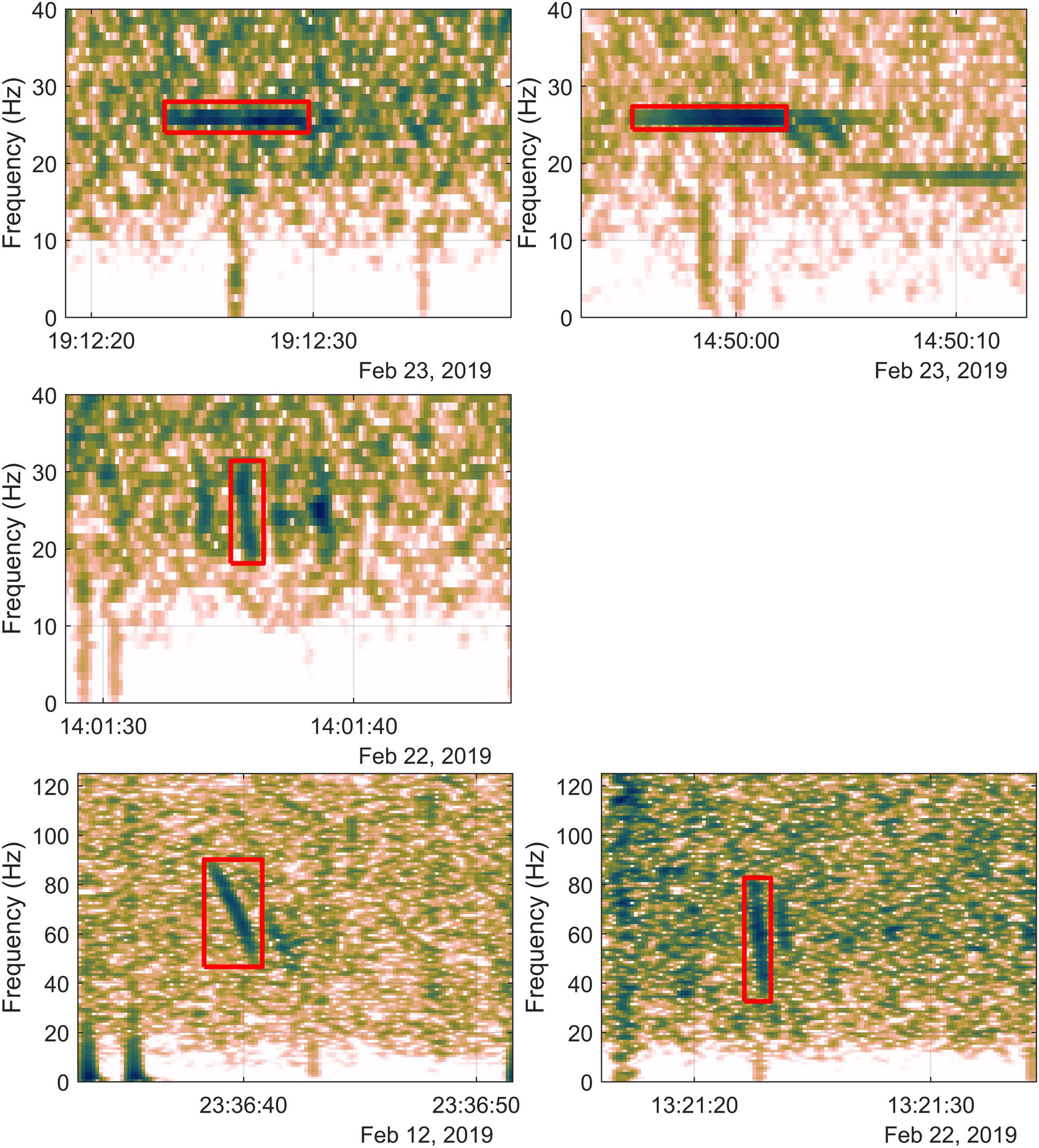
Figure 1. Examples of Antarctic blue whale (ABW) and fin whale calls recorded during the 2019 ENRICH voyage: ABW stand-alone unit-A (top left), ABW Z-call (top right), fin whale 20 Hz pulse (middle left) ABW D-call (bottom left), and fin whale 40 Hz downsweep (bottom right). Detection bounds for calls are indicated by the red square.

Location of Source

Georeferenced locations of whale calls (latitude and longitude) were obtained by performing additional analysis on the bearings obtained during the voyage from the PAMGuard-DIFAR module (Miller et al., 2016). This post-voyage analysis was performed in Matlab 2019b (Mathworks Inc., Natick, MA, United States). A combined detection-matching and localisation algorithm was used to estimate the call location.

For each detection, all detections on other sonobuoys that could potentially correspond to the same call were identified to determine which, if any, were the best match. A detection was considered a potential match if it was of the same sound type, its arrival occurred within the maximum time-differences-of-arrival (TDOAmax) for that pair of sonobuoys, and that detection had not previously been determined to match a different detection. TDOAmax was calculated from the known deployment locations of sonobuoys using a constant speed of sound (1400 m/s based on hydrographic sampling during the voyage). For recordings from pairs of sonobuoys, potential matches included all of the detections that arrived within TDOAmax on the second sonobuoy. For triplets, potential matches included all of the possible combinations of pairs of matches that arrived within TDOAmax on all three sonobuoys. For each set of candidate matches, the triangulated location was calculated via Lenth’s maximum likelihood method (Lenth, 1981). To apply Lenth’s method, latitude and longitudes were converted to cartesian coordinates (universal transverse Mercator projection) and triangulated positions converted back into latitudes and longitudes using the Matlab mapping package M_Map (Pawlowicz, 2019).

The TDOAs for each candidate location were then modelled assuming a constant sound speed of 1400 m/s. The candidate location where the modelled TDOAs best matched those calculated from the measured arrival times of each detection was accepted as the best matching location. Locations were only considered potentially acceptable if the mismatch between modelled and measured TDOA was less than 30% of the total maximum TDOA [i.e., Σ(TDOAmodelled − TDOAmeasured) ≤ 0.3 ΣTDOAmax]. The threshold for exclusion of 30% of the total TDOAmax was chosen to reject grossly mismatched detections whilst accommodating the three main sources of errors in TDOA: (1) sonobuoys that had drifted away from their deployment locations, (2) variability in the analysts’ marking of the time bounds of each detection, and (3) lack of coherence between detections arising from differing propagation conditions. Since triplets of sonobuoys were always likely to have a worse total match than any one of the three pairs of sonobuoys they contained, potential matches from triplets of sonobuoys were all calculated first, and pairs were only investigated if no triplet candidates were above the exclusion threshold.

Additional filters were applied to exclude poor triangulations and facilitate accurate estimation of source levels. Triangulations where whales or sonobuoys were in waters shallower than 1000 m were excluded due to our inability to model these TL accurately (see next section). Furthermore, we excluded triangulations that were greater than 50 km from the sonobuoy as these were likely to be inaccurate since they were more than three times further than our typical sonobuoy separation of 15–20 km. On the other end of the distance scale, we also excluded triangulations that were within 2 km of a sonobuoy, since these were more likely produce larger errors in TL and SL resulting from sonobuoys drifting away from their deployment locations.

Lastly, we considered the maximum angle of intersection, θ, of the bearings of each triangulation. Assuming that errors in bearings are symmetric around the true mean, then distant triangulations from bearings that are closer to parallel are more likely to be biased further away than those that are at right angles. Thus, SL that include these near-parallel bearings could be biased high. To check whether this occurred in our dataset, we investigate SL for an additional subset of calls where the angle of intersection of bearings, θ, was within 45° of a right angle (i.e., sin θ < 0.71). This subset of triangulations should be comparatively free of any bias that may arise from the limited angular precision of sonobuoys.

Transmission Loss Estimation

To reduce uncertainty in our modelling of TL, we considered only the most stable sound propagation regime: deep-water propagation between a shallow source (whale) and shallow receiver (sonobuoy). Specifically, we included only data when the sonobuoy and call location were in waters deeper than 1000 m. At shallower seafloor depths, TL are expected to be more sensitive to the bathymetry and geoacoustic model of the seabed, so would be expected to generate less accurate TL and SL.

Transmission loss modelling was performed using the parabolic equation method via the software RAMGeo (Collins, 2002) as distributed in AcTUP (Duncan, 2005), a wrapper and interface to the Acoustics Toolbox (Porter, 2020). To estimate TL at different potential whale depths, we applied the principle of reciprocity (Jensen et al., 2011). Here our working definition of reciprocity is that the TL between source A and receiver B will be identical even if the locations of A and B are switched. For all propagation models, the source was modelled at the known depth of the sonobuoy, 140 m. The grid of receivers (whales) was modelled with 5 m depth resolution, and 10 m of range resolution. Antarctic blue whales are known to produce sounds at depths typically between 25 and 30 m when they are in the sub-Antarctic (Bouffaut et al., 2021), and other subspecies of blue whales are also known to produce sounds at similar depths, though singular (stand-alone) version of calls tends to be produced slightly shallower (Lewis et al., 2018). There is more variability in the estimates of the depths at which fin whales produce sound. These range from 10–15 m (Stimpert et al., 2015) to 50 m (Watkins et al., 1987). Here we considered a range of whale depths from 10 to 50 m to assess the sensitivity of our method to depth. We also consider in more detail TL models with whale depths of 20 m for stand-alone blue whale unit-A and D-calls; 25 m for blue whale unit-A in Z-calls, and 15 m for both fin whale call types as these depths represent our best guess of whale calling depth for each call type from these prior studies. For these models we present detailed histograms and residuals for the spatially mixed geoacoustic model (described below). TL for ABW unit-A, Z-calls, and fin whale 20 Hz pulses were modelled at a frequency of 25 Hz, while D-calls and 40 Hz pulses were modelled at a frequency of 50 Hz.

Transmission loss was modelled independently for each detection (i.e., measured RL). For each detection, seafloor depth was extracted from the etopo1 database (Amante and Eakins, 2009) along the bearing connecting the sonobuoy and call location. The distribution of depth ranges along each of these bathymetric profiles is summarized in Figure 2. The sound speed profile for that detection was then calculated from the ENRICH voyage CTD data that were nearest in time, usually within 24 h (Figure 2). Sound speeds were calculated from pressure (depth), salinity (conductivity), and temperature using the formula of Chen and Millero (1977). Since the CTD was deployed only to 1000 m, sound speeds extracted from the world ocean atlas (Boyer et al., 2018) were used to fill the remaining depths between 1000 m and the seafloor.

FIGURE 2

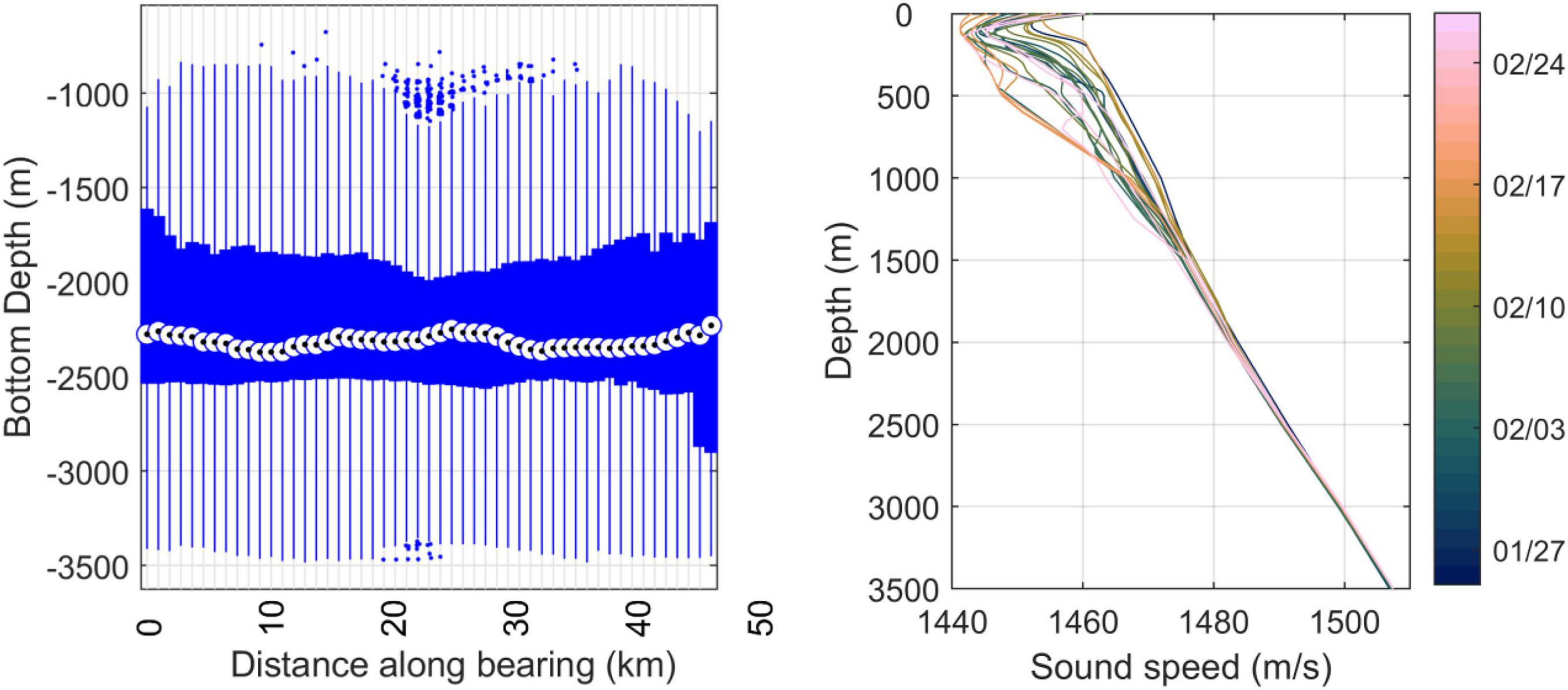
Figure 2. Left: Box and whisker plot of distribution of bathymetry along each of the 4155 triangulated bearings with sonobuoy at distance 0. Circle indicates median; box indicates 25–75 percentiles, whiskers indicate data limits, and outliers plotted as dots beyond the whiskers. Right: Sound speed profiles derived from the CTD casts during the 2019 ENRICH voyage (date collected is indicated by the colour bar).

Three different models of the geoacoustic properties of the seafloor were used, following the seabed sediment properties as described by Lurton (2010). The first model was meant to approximate highly porous sediments with large grain size (e.g., ooze, clay, mud) and here the seabed was assumed homogeneous with a compressional sound speed of 1500 m/s and density of 1200 kg/m3. The second model was meant to approximate less porous sediments with small grain size such as sand, and the seafloor was assumed homogenous with a compressional sound speed of 1749 m/s and density of 1941 kg/m3. The acoustic parameters for these models were based on the only geoacoustic data available for the study area: densities and sound speeds measured from sediment cores taken in the survey area during a geoscience voyage in 2000 (Brancolini and Harris, 2000). A third model was also considered that was a spatial mix of the first two models with the sediment type determined from the Census of Seafloor Sediments (Dutkiewicz et al., 2015). Here, the small-grain model was used when the Census of Seafloor Sediments indicated the sediments were “sand” at the whale location, and the large grain model was used everywhere else (Figure 3). Use of the parabolic equation and geoacoustic model meant that we did not need to calculate eigenrays, or make assumptions about whether a detection was a direct arrival or from a multipath surface or bottom reflection. As a reference solely for visual comparison purposes, we also plotted alongside each of our geoacoustic TL models, transmission loss resulting from simple spherical spreading (TL = 20 log₁₀r) and cylindrical spreading beyond a “transition range” of our mean depth of 2250 m: TL = 10 log₁₀ 2250 + 10 log₁₀r (Urick, 1983; Hall, 2005; Lurton, 2010).

FIGURE 3

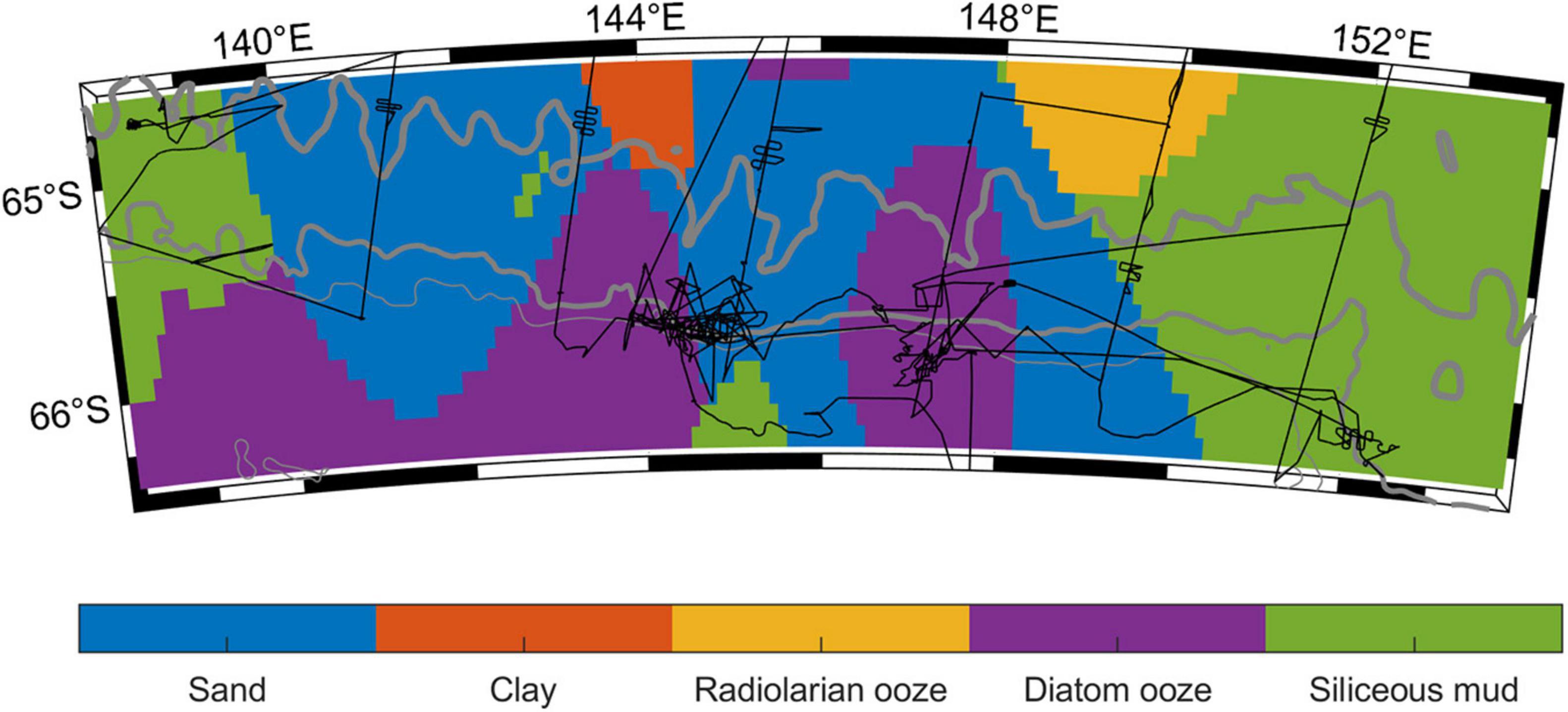
Figure 3. Map of seabed sediment types (coloured patches) from the Census of Seafloor Sediments (Dutkiewicz et al., 2015) for the portion of the ENRICH voyage track (black line) that contained locations of triangulated calls from Antarctic blue and fin whales. From thin to thick grey lines indicate the 1000, 2000, and 3000 m bathymetric depth contours.

Method Summary With an Example

We illustrate our method for estimating SL with real examples of each of the key steps for a pair of detections for a single call Figure 4. Different coloured panels in this figure illustrate features of the detection matching and localisation algorithm, environmental data, and propagation modelling for a single D-call. Here the TDOA measured between detection #1 on sonobuoy A and detection #2 on sonobuoy B is 7.70 s, and the TDOA estimated from the localisation from sonobuoy bearings is 7.00 s. Our tolerance (0.3 * TDOAmax) is 2.18, so these detections are deemed to be a match (reception of the same call). The RL and TL for this example illustrate the complexity of shallow-water high-latitude sound propagation. RLs were 108.9 dB, and 109.3 dB at detection #1 and detection #2, respectively. This is an interesting quirk because detection #1, which was only 3 km from the whale, had RL that was 0.4 dB lower than that from detection #2 which was nearly 13 km away. However, the larger TL of 86.0 vs. 84.4, respectively, at 20 m depth potentially provides some explanation. The addition of RL and TL yielded SL of 195.0 and 193.7 for detection #1 and detection #2, respectively. Thus, our estimate of SL for the call is 194.3 and our estimate of measurement error, σ_∈, is 0.92 for this call. In this example, detection #2 appears to consist of obvious multipath arrivals. Looking closely at the spectrogram, one can see a faint copy of the call preceding the detection. This faint preceding call is most likely the direct arrival, but could also be a weaker multi-path. None of these seeming irregularities pose any problem for our methods, however, they are worth noting because they could cause problems for algorithms that require common assumptions about arrival order or TL (e.g., assumption that all detections are direct arrivals, or assumption that there is a monotonic decreasing relationship between TL and distance).

FIGURE 4

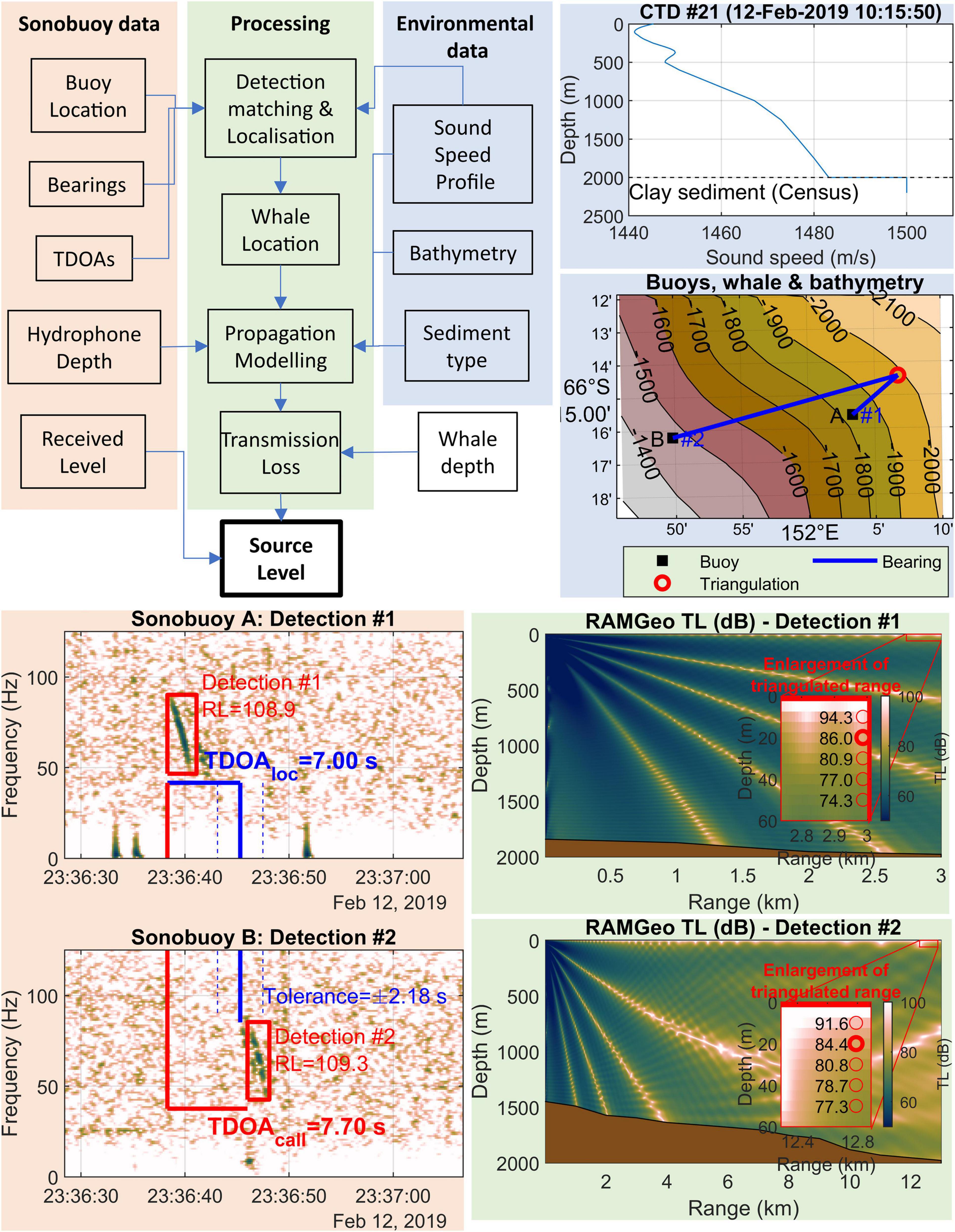
Figure 4. Flowchart showing overview of methods used to estimate source level (top left). Remaining panels show illustrated example of key steps for an example D-call that was detected on a pair of sonobuoys, which we label (A) and (B). Background colours of panels correspond to those of the flowchart: pink for “Sonobuoy data,” blue for “Environmental data,” and green for “Processing.” Bottom left: spectrogram illustrating the time-frequency bounds for the detection #1 on sonobuoy A and detection #2 on sonobuoy B (red boxes). Time difference of arrival (TDOA) calculated from the start of each detection are shown as red-lines and TDOA_loc (estimated TDOA from bearing triangulation) shown as solid blue lines. These TDOAs are within our tolerance (dashed blue line), so these detections are deemed to be from the same call. Top right: Sound speed profile derived from voyage CTD cast and seafloor speeds derived from census of marine sediments. Middle right: map showing bathymetry (depths contours in m), sonobuoy deployment locations, bearings to detection #1 and #2, and the triangulated whale location (red circle). Bathymetry and distances for transmission loss (TL) modelling are extracted along bearings (blue lines). Bottom right panels show the output of two TL models (range, depth, and TL) for the example call along bearings detection #1 (upper RAMGeo TL plot) and detection #2 (bottom RAMGeo TL plot). The red box and inset plot show an expanded view of TL model over the range of potential whale depths we considered in this study (10–50 m); circles are marking every 10 m of depth increments with text representing modelled value of TL at that depth. The bold circle indicates our “best guess” for whale depth for this call type (20 m) based on whale depths reported in previous studies.

Results

Received Levels and Source Locations

During 205 h of concurrent acoustic recordings from multiple sonobuoys (150 h of 2-audio-channel and 55 h of 3-audio-channel recordings), 1915 calls met all of our criteria for SL estimation, including 532 unit-A calls, 350 complete Z-calls, 850 D-calls, 62 20 Hz pulses, and 121 40 Hz downsweeps measured over 19, 14, 18, 7, and 12 recording-days, respectively (Table 1). The locations of these calls were predominantly south of 65°S, over the continental slope, and adjacent deeper waters (Figure 5). RLs of triangulated calls ranged from 93 to 125 dB re 1 μPa. Unlike the results of Širović et al. (2007), our RLs did not show a clear trend with log of distance as would be expected for a source at fixed depth with constant SL and with a TL that follows a simple geometric spreading law of the form X log r (Figure 5). Nor did our RL appear to closely follow a simple analytical model of cylindrical spreading in a surface duct with a transition range of r₀, such that TL = 10 log10 r₀ + 10 log10 r (Urick, 1983; Hall, 2005; Lurton, 2010).

TABLE 1

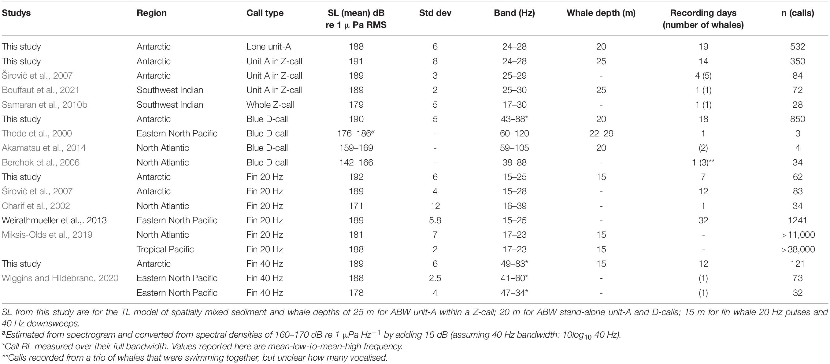
Table 1. Estimates of source levels of Antarctic blue whale (ABW) and fin whale calls estimated during ENRICH 2019, and other studies.

FIGURE 5

Figure 5. Left column: Maps of locations of triangulated calls used for estimation of SL with colour bar indicating the date of recording (each panel shows only a single call type). From thin to thick grey lines indicate the 1000, 2000, and 3000 m bathymetric depth contours. Right: Received level of triangulated detections as a function of distance from the sonobuoy deployment location, with blue dots showing the full dataset, and orange dots showing the subset of data where intersection angle of triangulations were within 45° of a right angle and thus expected to be free of bias arising from limited angular precision.

Transmission Loss Modelling Inputs

Mean depth along the 4155 bathymetric profiles used in TL modelling was 2250 m, and sound-speeds ranged from 1441 to 1508 m/s across all CTD casts (Figure 2). The depth of the sound-speed minimum ranged from 40 to 160 m across all CTD casts, with a median of 110 m (Figure 2). According to the census of marine sediments (Dutkiewicz et al., 2015) approximately 25% of the triangulated detections were located over sand (Figure 3).

The different geoacoustic models yielded substantially different estimates of TL, with the clay model leading to highest TL, the sand model leading to lowest TL, and the mixed geoacoustic model yielding intermediate results, but closer to the clay model (Figure 6).

FIGURE 6

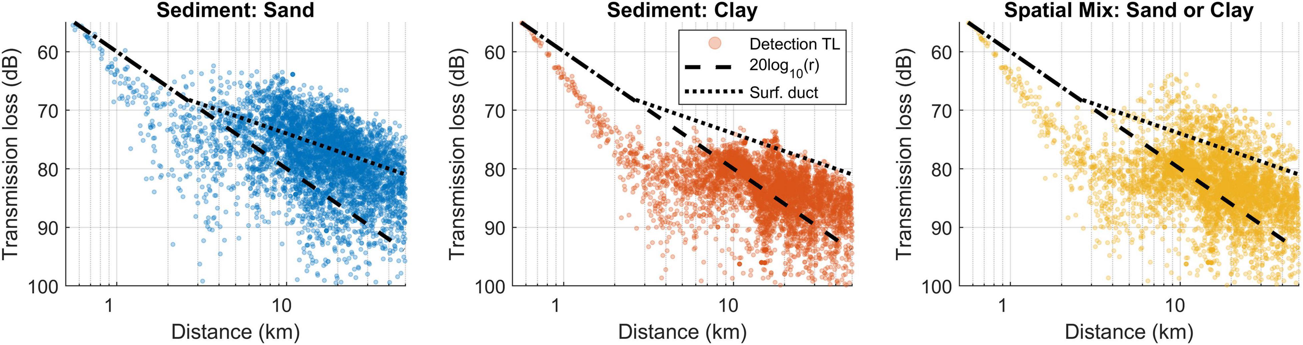
Figure 6. Transmission loss (TL) as a function of distance for each triangulated detection with seafloor sediments modelled as sand (left), clay (middle), and as either sand or clay spatially according to the Census of Seafloor Sediments (Dutkiewicz et al., 2015) (right panel). Black lines show simple analytical models of spherical spreading (20 log₁₀ r; dashed line), and a surface duct (10log₁₀ 2500 + 10log₁₀ r), i.e., a duct with a transition range of 2.5 km (dotted line).

Source Levels

The geoacoustic model and modelled depth of whale had a strong influence on SL. The higher TL of the “clay” geoacoustic model yielded higher SL, and vice-versa for the lower TL of the “sand” geoacoustic model. Shallower whale-depths yielded larger SL across all geoacoustic models (Figure 7). However, the differences in SL among the three geoacoustic models were largest at shallow depths and decreased as whale depth increased.

FIGURE 7

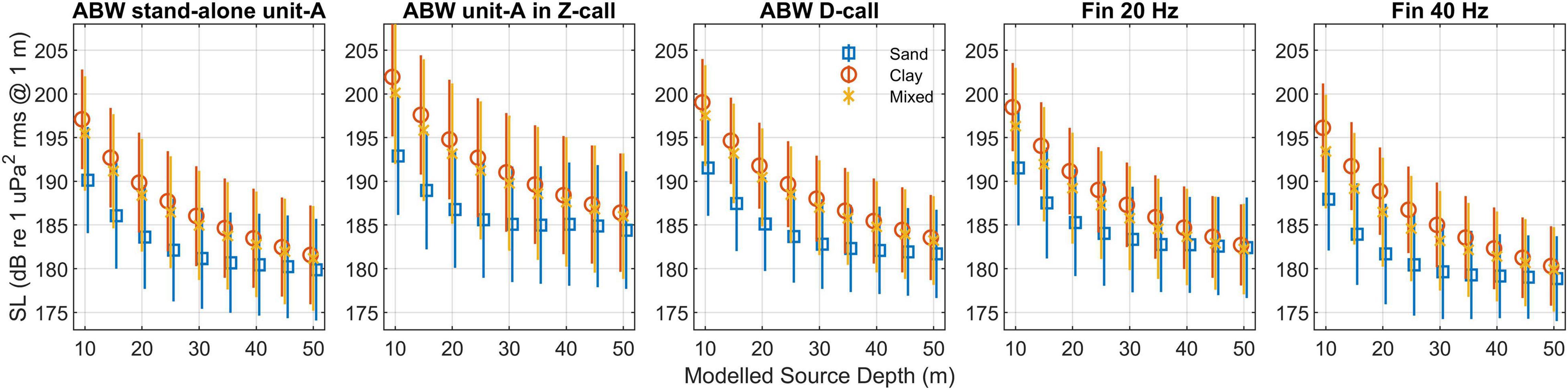
Figure 7. Mean SL as a function of depth for three different geoacoustic models: sand (blue squares), clay (red circles), and spatial mix of sand or clay (orange cross). Error bars indicate ± one standard deviation. Colours are the same as the TL models in Figure 6.

The assumptions about whale calling depth had the largest effect on estimated TL and consequently SL. For all call types SL estimates were 15–20 dB higher if the whale was assumed to be calling at a depth of 10 m compared to 50 m (Figure 7). For our best guess of whale depth and geoacoustic model, SL across all call types ranged from 188 to 192 dB, with standard deviations of calls ranging between 5.5 and 7.8 dB and measurement error, σ_∈, ranging from 5.7 to 6.7 dB (Figure 8). SL for the subset of triangulations with intersection angles near right-angles were 2–3 dB lower than the full datasets for respective call types, except for unit-A within a Z-call, which was 1 dB higher (Figure 8).

FIGURE 8

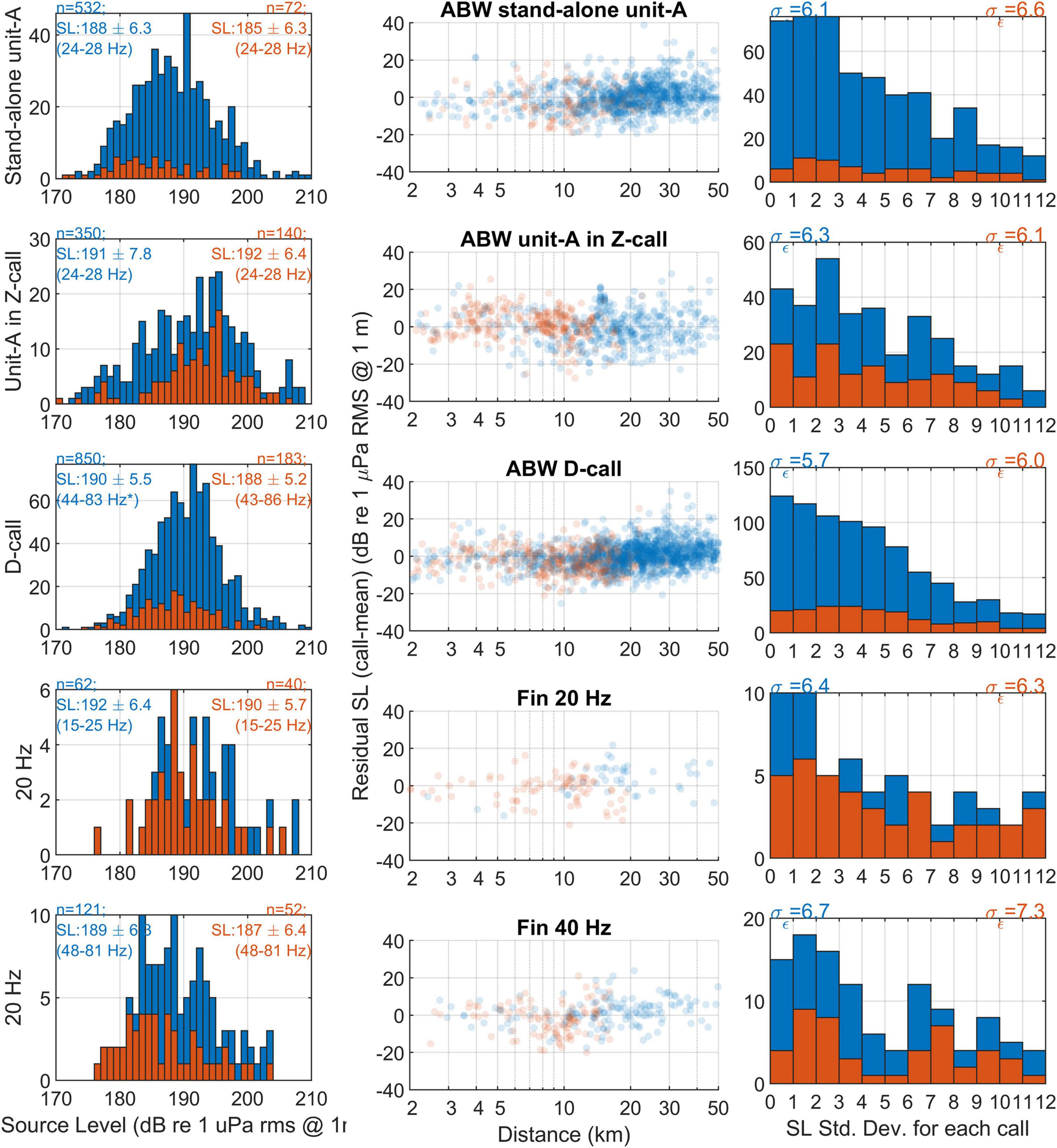
Figure 8. Left column: histograms of source levels of Antarctic blue whale and fin whale calls derived from spatially mixed TL model with source depth of 25 m for unit-A in Z-call, 20 m for stand-alone unit A and D-calls, and 15 m for 20 Hz and 40 Hz calls. Middle: Scatter plot of residual SL (SL_call - mean) as a function of distance for this TL model and whale depth. Right: distribution of standard deviation of measurement errors, σ_∈, from each individual call. In all columns, blue colour is used for the full dataset, and orange colour indicates the subset of data where intersection angle of triangulations were within 45° of a right angle and thus expected to be free of bias arising from limited angular precision.

Discussion

Comparison With Other Studies

For models where whale depths for each call type corresponded closely to those reported in previous studies (20 m depth for stand-alone unit-A and D-calls, 25 m for unit-A in Z-calls, 15 m for fin whale 20 and 40 Hz calls), mean SL measured in our study were all within 4 dB of each other. Our modelled SLs at our best estimate of whale depth for each call type were broadly similar to previous estimates in the Antarctic (Figure 8 and Table 1). Our estimates of SL of unit-A within a Z-call was 2 dB higher than previous estimates which both had a mean of 189 dB (Širović et al., 2007; Bouffaut et al., 2021), however, they are all within standard deviations of these other measurements. Our estimates of stand-alone unit-A of 188 dB is the first estimate of SL for this call. Compared to SL of unit-A produced within a Z-call it is 3 dB lower than our estimate from this study, and 1 dB below previous studies (Širović et al., 2007; Bouffaut et al., 2021). Our estimate of a mean SL of 192 dB for fin 20 Hz pulses was 3 dB higher than previous estimates of 189 dB made in the Antarctic and elsewhere (Širović et al., 2007; Weirathmueller et al., 2013), but again within standard deviations. Our estimate of SL of 190 for D-calls was considerably higher than calls that were measured in the North Atlantic (Berchok et al., 2006; Akamatsu et al., 2014). Thode et al. (2000) presented source spectrograms of 3 D-calls with spectral densities between 160 and 170 dB re 1 μPa Hz^–1 from 40 to 80 Hz. Converting these to comparable units by adding 10log₁₀(B), where bandwidth, B = 40 Hz, we obtain an SL of 176–186 dB. Our estimate of 190 is 4 dB above the high end of that range. Our SL of 189 dB for fin whale 40 Hz downsweeps are the first published estimate of SL for this call type in the Southern Hemisphere. These appear to be similar to the higher of the two measurements reported in the Northern Hemisphere (Wiggins and Hildebrand, 2020).

Though we have focused on the calls of Antarctic blue and fin whales on their Antarctic feeding grounds, our method for estimating SL from sonobuoy detections should be generally applicable to other call types and environments – provided that there is sufficient environmental information to model TL with fidelity. Due to only having coarse information of seabed geoacoustics from a survey two decades prior, we opted not to include shallow water localisation in our results. Our inclusion of only deep-water detections could potentially result in censoring bias if whales change SL in response to water depth. However, Miksis-Olds et al. (2019) provide an illustrative example of the difficulties of SL estimation in shallow water without sufficient knowledge of seabed geoacoustics, so SL of blue and fin calls in shallow water remains a knowledge gap for future studies to address.

The only component of our method that is not general-purpose is our localisation and detection matching algorithm, which makes use of direction of arrival via the sonobuoys acoustic vector sensors. However, use of bearings in our localisation algorithm only served to simplify the logistics of deploying our arrays by allowing for localisations from as few as two sensors and by simplifying time-synchronisation since signals from all sonobuoys were recorded simultaneously on the same analog-to-digital converter using the same clock. In comparison TDOA methods typically require 3, if not more, omnidirectional sensors for effective localisation (Møhl et al., 2001; Spiesberger, 2001; Thode et al., 2006; Baumgartner et al., 2008; Miller and Dawson, 2009), and also often require additional hardware or software-processing for accurate time synchronisation (Møhl et al., 2001; Thode et al., 2006). Assuming that there is sufficient hardware to obtain a localisation (via bearings, TDOA, or some combination of the two), then our remaining methods, e.g., for measuring RL and estimating TL, can all be applied more broadly to any relatively narrow-band low-frequency sounds in almost any marine environment without modification. For calls that have larger bandwidth than those of blue and fin whales, broadband propagation modelling may need to be considered (see Helble et al., 2013 for an example of how such methods might be developed and applied). Furthermore, the general-purpose methods we presented are not mutually exclusive with other localisation algorithms. Thus, future studies could investigate the use of multipath, either independently (Bouffaut et al., 2021) or alongside bearings and TDOAs and propagation modelling (Nosal and Frazer, 2007) in order to better estimate range, depth, bottom composition, and measurement error.

Regardless of geoacoustic model, and regardless of whale depth, the variability in our SL was larger than previous estimates of ABW unit-A, similar to variability reported for blue whale D-calls, in the middle of the pack for fin whale 20 Hz pulses, and higher than the two estimates of SL for 40 Hz pulses (Table 1). This suggests that the precision of our SL estimates is either lower than some of the other methods, or there is more natural variation in SL (or whale calling depth) than has been captured in previous studies of Southern Hemisphere whales. The Gaussian distribution of SL for the signals measured in this study suggests that there could be a natural range of SL produced by blue and fin whales and further that this range may naturally vary with animal depth. This makes sense from a physiological perspective since every 10 m of depth results in an increase of 1 atm (100 kPa) of pressure, potentially constraining the SL of an air-based sound source as has been proposed for blue whales (Aroyan et al., 2000; Dziak et al., 2017).

Sources of Variability and Error

The variability in our SL estimates comprises natural variability in the source level as produced by the animals, as well as errors in our measurements and models. Quantifying the amount of natural variability both within individuals and among different whales would be biologically interesting. However, within our results, we are unable to separate natural variability from errors in our measurements and models because variability from measurement error, σ_∈ was similar in magnitude to the total variability across all calls σ. The main sources of measurement and modelling error in our study include: errors in measuring received level, errors in localisation, and mismatch of TL models with reality.

Errors in Received Level Measurement

By following a strict protocol in determining the start, stop and frequency band of each detection and excluding calls that contain obvious noise sources we have reduced the measurement error on our RLs as much as possible. The theoretical limit for our RL measurements is the acoustic calibration of the DIFAR omnidirectional sensor, and this is only specified accurate to within ±3 dB.

Localization Error

Localization errors arise from inaccurate sonobuoy locations (e.g., due to buoys drifting away from deployment location), and inaccurate/imprecise bearings. To provide accurate locations relative to the array, sonobuoys are designed (with a drogue and low windage at the surface) to drift at the same speed and direction so long as they are in the same water mass. Thus, assuming our array deployments were in the same water mass, the main source of differential drift between buoys arises from the difference in deployment times. During the ENRICH voyage, that mean difference in deployment times between sonobuoys that formed a pair was 2.4 h. While the low self-noise levels of RV Investigator (Duncan et al., 2015) throughout the voyage made a great platform for listening for blue and fin whale sounds, it also restricted our options for calibrating the sonobuoy compass (Miller et al., 2016), and estimating drift using ship noise (Miller et al., 2018). Since estimation of SL depends heavily on accurate knowledge of the relative and absolute locations of both source and receivers, we believe this is the most limiting source of error. Furthermore, localization errors will compound errors in modelling of TL since environmental parameters will be incorrect if locations are not correct. While localization errors ultimately limit the precision of our SL estimates, our investigation of bias arising from near-parallel bearings suggested that limited angular precision of sonobuoys was not a major source of bias in our study. Mean SLs from our full dataset were within +1 to −3 dB of our “unbiased” subset of calls (where intersection angle of bearings were all within 45° of right-angles). Thus, bias from limited precision of bearings appears to be smaller than errors arising from incorrectly modelled whale-depth (up to 20 dB) or geoacoustic model (up to 7 dB). Future studies using sonobuoys with in-built GPS positioning would alleviate localization errors due to drift. However, GPS-enabled sonobuoys are not yet regularly available for use by the marine bioacoustics community.

Modelling Errors

While ray-tracing has been used in a few studies to model TL of low-frequency, long-travelling blue whale calls (Širović et al., 2007; Shabangu et al., 2020; Bouffaut et al., 2021), the parabolic equation method we used is a more appropriate and tractable approach for scenarios, such as the ENRICH voyage, where variable bathymetry must be taken into account (Lurton, 2010; Etter, 2012; Farcas et al., 2016). The use of a numerical method based on the parabolic equation, along with real-world sound speed profiles means that there is no need to separately model phenomena such as the Lloyd’s Mirror effect (discussed in detail for this context by Bouffaut et al., 2021). Instead, these phenomena should become emergent properties of a numerical model, with the Lloyd’s Mirror effect, in particular, commonly used as a benchmark of the accuracy of most numerical methods (Jensen et al., 2011).

Since the parabolic equation method has been validated as accurate, and recommended as the most appropriate model for our scenario (Etter, 2012; Farcas et al., 2016), errors in our models of TL are believed to predominantly arise from mismatch between the model parameters and the actual environment rather than from the mathematics of the model itself. Our strategy for controlling this source of error was to model TL for each bearing independently using the best available information. The sound-speed profiles in our models came from in-situ CTD casts, usually on the same day and not too distant from most of our detections. In-situ sound-speed profiles should be more accurate and representative of in-situ propagation than reliance on climatologies such as the world-ocean atlas, or GDEM-V (Mountain et al., 2013; Boyer et al., 2018). The etopo1 bathymetry (Amante and Eakins, 2009) that we used had 1 arc-minute spatial resolution. While higher resolution bathymetry does exist for some portions of our voyage (e.g., the area along the ENRICH voyage track), we suspect diminishing-to-null improvement from using better bathymetry because the accuracy of the absolute source and receiver locations is limited by the accuracy of measured bearings, sonobuoy drift and compass calibrations (as explained above).

Even without addressing localization errors, there is potential to improve our estimates of SL if a more accurate geoacoustic model of the seafloor were available. Modelling the seabed as sand resulted in TL measurements that were on-average 4–7 dB lower than modelling the seabed as clay, and 3–6 dB lower than a spatial mix of sand and clay across all call types (Figure 7). The spatially mixed model following Census of Seafloor Sediments was intended to represent our best guess of seabed geoacoustic properties. However, this set of models had nearly three times as many sediments modelled as clay than sand, so ultimately yielded results similar to the clay model, but with greater variability in TL than either of the single-sediment models. We suggest that this increased variability appropriately reflects some of the uncertainty in our geoacoustic modelling of the seabed.

The last potential source of error arises from error in the modelled calling depth of the whale. Though potentially a localization error, it is listed here because our localizations are 2D and whale depth is a parameter used in our models of TL. Previous studies of calling depth of blue and fin whales indicate that most calls are produced between 15 and 30 m deep, and here we assume that this is true in the Antarctic (Thode et al., 2000; Stimpert et al., 2015; Lewis et al., 2018; Bouffaut et al., 2021). More precise knowledge of calling depth would improve the accuracy of our SL estimates. The median difference in TL across all calls between assuming a calling depth of 20 m compared to 30 m was 3.7 dB (s.d. = 1.4 dB). Thus, calling depth could account for a large proportion of the variability we observed in estimated SL. The variance in the difference in TL between different calling depths was small compared to the difference itself. This suggests that for understanding RL and detection probability as a function of distance for the oceanographic conditions in our study area, a combination of assumed call depth and estimated SL is important. Hence estimates of SL should also specify the assumed calling depth. Future studies could also investigate the integration of multipath localisation methods alongside our methods to estimate calling depth from the acoustic and environmental data (Nosal and Frazer, 2007; Bouffaut et al., 2021).

Advantages of Using Sonobuoys for Source Level Measurements

While there are clearly limitations with the precision of SL estimates made using sonobuoys, a key advantage is that sonobuoys deployed as part of a dedicated cetacean research program provide more opportunities to estimate SL than tags on individual animals (small sample size), dipping hydrophone recordings (which rely on assumptions about the underwater behaviour of animals seen at the surface) or even single fixed hydrophones (where precise locations of calling whales are generally unavailable). Our SL for Antarctic blue whale sounds were estimated from a much larger number of calls than previous studies, and a similar number of fin whale calls as previous Southern Hemisphere studies, even though fin whales were not the primary research focus during the voyage. In addition to a higher number of calls, our estimates came from a larger number of recording sessions/different days, a typical proxy for number of individual animals.

Conclusion

We have demonstrated a viable method of estimating source levels of baleen whale calls from arrays of DIFAR sonobuoys. Application of this method to recordings of Antarctic blue and fin whales from an Antarctic voyage provided the first estimates of the SL of blue whale D-calls from the Antarctic, and the first Southern Hemisphere estimate of SL of fin whale 40 Hz downsweeps. Additionally, this dataset comprises the largest sample of Antarctic blue whale song calls used for SL estimation to-date. Our estimates of SL for blue and fin whale calls were similar in magnitude, but in some cases had more variability than previous studies. The additional variability could potentially arise from natural variability (e.g., from using a larger number of calls from a larger number of individuals), but is also likely due to localization errors and limited environmental inputs into models of TL. Despite these constraints, the contribution of a statistically robust distribution of SL for multiple call types from two species is of value with regards to estimating the relative density of animals from single hydrophones. Understanding the natural variability within a population will lead to more accurate, if less precise call density estimates. At the same time, the variability highlights the limitations of density estimation based on relatively few inputs and suggests that while such estimates are valuable, they need to be considered in the context of currently limited understanding of biological and environmental variation.

Data Availability Statement

The datasets presented in this study can be found in online repositories. The names of the repository/repositories and accession number(s) can be found below: ENRICH voyage data: NCMI Information and Data Centre – https://www.cmar.csiro.au/data/trawler/survey_details.cfm?survey=IN2019%5FV01; ENRICH sonobuoy data: Australian Antarctic Data Centre – https://data.aad.gov.au/metadata/records/AAS_4600_ENRICH_Sonobuoy_Data (Miller et al., 2021b).

Ethics Statement

The animal study was reviewed and approved by the Australian Government, Department of Environment and Energy, under Cetacean Permit 17-0004 under the Environment Protection and Biodiversity Conservation Act 1999 (EPBC); Permit AMLR 18-19-4101-INVESTIGATOR under the Antarctic Marine Living Resources Conservation Act 1981; and a notice of Determination and Authorisation under the Antarctic Treaty (Environment Protection) Act 1980 (ATEP) issued on September 27, 2018.

Author Contributions

BM, SC, RL, EM, AŠ, and KS: concept and methods. BM, SC, EM, AŠ, and KS: collect and process data. EB, MD, BM, AŠ, and KS: funding. MD, EB, and BM: voyage management. BM and RL: additional analysis. BM, SC, RL, KS, EM, AŠ, and EB: write and edit manuscript.

Funding

This work was conducted as part of the Australian Antarctic Program under Australian Antarctic Science Projects 4101, 4102, and 4600. Participation of KS and AŠ in this work was funded in part by IWC-SORP grant “Acoustic Ecology of Foraging Antarctic Blue Whales in the Vicinity of Antarctic Krill Studied During AAD Interdisciplinary Voyage Aboard the RV Investigator” and NSF-OPP award 1745930. Thanks to the hard-working and very professional crew of RV Investigator, and thanks to the CSIRO Marine National Facility (MNF) for its support in the form of sea time on RV Investigator, support personnel, scientific equipment, and data management. All data and samples acquired on the voyage are made publicly available in accordance with MNF Policy.

Conflict of Interest

The authors declare that the research was conducted in the absence of any commercial or financial relationships that could be construed as a potential conflict of interest.

Publisher’s Note

All claims expressed in this article are solely those of the authors and do not necessarily represent those of their affiliated organizations, or those of the publisher, the editors and the reviewers. Any product that may be evaluated in this article, or claim that may be made by its manufacturer, is not guaranteed or endorsed by the publisher.

Acknowledgments

Thanks to Karen Westwood for voyage management during planning, and to Nat Kelly for designing the ENRICH transects and for discussions on how the passive acoustics work would fit into the broader voyage objectives. Thanks to Steve Whiteside, Mark Milnes, Kym Newberry, and all the Australian Antarctic Division Science Technical Support personnel, whose contributions and excellent support provided for the success of this work and the voyage. Thanks to the IWC-SORP Acoustic Trends Steering Group for sharing their thoughts and support in planning the passive acoustics work during the voyage.

References

Akamatsu, T., Rasmussen, M. H., and Iversen, M. (2014). Acoustically invisible feeding blue whales in Northern Icelandic waters. J. Acoust. Soc. Am. 136, 939–944. doi: 10.1121/1.4887439

CrossRef Full Text | Google Scholar

Amante, C., and Eakins, B. W. (2009). ETOPO1 1 Arc-Minute Global Relief Model: Procedures, Data Sources and Analysis. NOAA Technical Memorandum NESDIS NGDC-24. Washington, DC: National Geophysical Data Center, NOAA. doi: 10.7289/V5C8276M

CrossRef Full Text | Google Scholar

Andrews-Goff, V., Olson, P. A., Gales, N. J., and Double, M. C. (2013). Satellite Telemetry Derived Summer Movements of Antarctic Blue Whales. Report SC/65a/SH03 submitted to the Scientific Committee of the International Whaling Commission. Jeju Island: International Whaling Commission.

Google Scholar

Aroyan, J., McDonald, M. A., Webb, S. C., Hildebrand, J. A., Clark, D., Laitman, J. T., et al. (2000). “Acoustic models of sound production and propagation,” in Hearing by Whales and Dolphins, eds W. W. L. Au, A. N. Popper, and R. R. Fay (New York, NY: Springer), 409–469.

Google Scholar

Baumgartner, M. F., Freitag, L., Partan, J., Ball, K. R., and Prada, K. E. (2008). Tracking large marine predators in three dimensions: the real-time acoustic tracking system. IEEE J. Ocean. Eng. 33, 146–157. doi: 10.1109/JOE.2007.912496

CrossRef Full Text | Google Scholar

Bell, E. M. (2021). Annual Report of the Southern Ocean Research Partnership (IWC-SORP) 2020/21. Paper Submitted to Scientific Committee of the International Whaling Commission SC68C, 90. Cambridge: International Whaling Commission.

Google Scholar

Berchok, C. L., Bradley, D. L., and Gabrielson, T. B. (2006). St. Lawrence blue whale vocalizations revisited: characterization of calls detected from 1998 to 2001. J. Acoust. Soc. Am. 120:2340. doi: 10.1121/1.2335676

CrossRef Full Text | Google Scholar

Bouffaut, L., Landrø, M., and Potter, J. R. (2021). Source level and vocalizing depth estimation of two blue whale subspecies in the western Indian Ocean from single sensor observations. J. Acoust. Soc. Am. 149, 4422–4436. doi: 10.1121/10.0005281

CrossRef Full Text | Google Scholar

Boyer, T. P., Garcia, H. E., Locarnini, R. A., Zweng, M. M., Mishonov, A. V., Reagan, J. R., et al. (2018). World Ocean Atlas 2018. NOAA Natl. Centers Environ. Information. Available online at: https://accession.nodc.noaa.gov/NCEI-WOA18 (accessed August 3, 2021).

Google Scholar

Branch, T. A. (2007). Abundance of Antarctic blue whales south of 60 S from three complete circumpolar sets of surveys. J. Cetacean Res. Manag. 9, 253–262.

Google Scholar

Branch, T. A., and Butterworth, D. S. (2001). Estimates of abundance south of 60^° S for cetacean species sighted frequently on the 1978/79 to 1997/98 IWC/IDCR-SOWER sighting surveys. J. Cetacean Res. Manag. 3, 251–270.

Google Scholar

Branch, T. A., Stafford, K. M., Palacios, D. M., Allison, C., Bannister, J. L., Burton, C. L. K., et al. (2007). Past and present distribution, densities and movements of blue whales Balaenoptera musculus in the Southern Hemisphere and northern Indian Ocean. Mamm. Rev. 37, 116–175. doi: 10.1111/j.1365-2907.2007.00106.x

CrossRef Full Text | Google Scholar

Brancolini, G., and Harris, P. (2000). Post-Cruise Report AGSO Survey 217?: Joint Italian/Australian Marine Geoscience Expedition Aboard the R.V. Tangaroa to the George Vth Land Region of East Antarctica during February-March, 2000: Australian National Antarctic Research Expeditions Project no. 1044, Wilkes Land Glacial History (WEGA). Canberra, ACT: Commonwealth of Australia.

Google Scholar

Buchan, S. J., Gutierrez, L., Balcazar-Cabrera, N., and Stafford, K. M. (2019). Seasonal occurrence of fin whale song off Juan Fernandez, Chile. Endanger. Species Res. 39, 135–145. doi: 10.3354/esr00956

CrossRef Full Text | Google Scholar

Calderan, S., Black, A., Branch, T., Collins, M., Kelly, N., Leaper, R., et al. (2020). South Georgia blue whales five decades after the end of whaling. Endanger. Species Res. 43, 359–373. doi: 10.3354/esr01077

CrossRef Full Text | Google Scholar

Charif, R. A., Mellinger, D. K., Dunsmore, K. J., Fristrup, K. M., and Clark, C. W. (2002). Estimated source levels of fin whale (Balaenoptera physalus) vocalizations: adjustments for surface interference. Mar. Mamm. Sci. 18, 81–98. doi: 10.1111/j.1748-7692.2002.tb01020.x

CrossRef Full Text | Google Scholar

Chen, C.-T., and Millero, F. J. (1977). The sound speed in seawater. J. Acoust. Soc. Am. 62, 1129–1135.

Google Scholar

Clark, C. W., Ellison, W. T., Southall, B. L., Hatch, L., Van Parijs, S. M., Frankel, A. S., et al. (2009). Acoustic masking in marine ecosystems: intuitions, analysis, and implication. Mar. Ecol. Prog. Ser. 395, 201–222. doi: 10.3354/meps08402

CrossRef Full Text | Google Scholar

Collins, M. D. (2002). User’s Guide for RAM Version 1.0 and 1.0p. Available online at: http://oalib.hlsresearch.com/AcousticsToolbox/ (accessed August 2, 2021).

Google Scholar

Cooke, J. G. (2018a). Balaenoptera musculus ssp. Intermedia. IUCN Red List Threat. Species, e.T41713A50226962. Available online at: https://dx.doi.org/10.2305/IUCN.UK.2018-2.RLTS.T41713A50226962.en (accessed August 25, 2021).

Google Scholar

Cooke, J. G. (2018b). Balaenoptera physalus (Fin whale). Balaenoptera physalus. Available online at: https://dx.doi.org/10.2305/IUCN.UK.2018-2.RLTS.T2478A50349982.en (accessed August 25, 2021).

Google Scholar

Double, M. C. (2019). Euphausiids and Nutrient Recycling in Cetacean Hotspots (ENRICH) Voyage Report. Report in preparation. Kinsgston, TAS: Australian Antarctic Division.

Google Scholar

Duncan, A. (2005). Acoustics Toolbox User interface adn Post processor (AcTUP). Available online at: http://cmst.curtin.edu.au/products/underwater/ (accessed August 2, 2021).

Google Scholar

Duncan, A., Kloser, R., and Sherlock, M. (2015). “Measurements of underwater noise from the RV investigator,” in Proceedings of Acoustics 2015, (Hunter Valley, NSW: Australian Acoustical Society), 1–9.

Google Scholar

Dutkiewicz, A., Müller, R. D., O’Callaghan, S., and Jónasson, H. (2015). Census of seafloor sediments in the world’s ocean. Geology 43, 795–798. doi: 10.1130/G36883.1

CrossRef Full Text | Google Scholar

Dziak, R. P., Haxel, J. H., Lau, T.-K., Heimlich, S., Caplan-Auerbach, J., Mellinger, D. K., et al. (2017). A pulsed-air model of blue whale B call vocalizations. Sci. Rep. 7:9122. doi: 10.1038/s41598-017-09423-7

PubMed Abstract | CrossRef Full Text | Google Scholar

Edwards, E. F., Hall, C., Moore, T. J., Sheredy, C., and Redfern, J. V. (2015). Global distribution of fin whales Balaenoptera physalus in the post-whaling era (1980-2012). Mamm. Rev. 45, 197–214. doi: 10.1111/mam.12048

CrossRef Full Text | Google Scholar

Etter, P. C. (2012). Advanced applications for underwater acoustic modeling. Adv. Acoust. Vib. 2012:214839. doi: 10.1155/2012/214839

CrossRef Full Text | Google Scholar

Farcas, A., Thompson, P. M., and Merchant, N. D. (2016). Underwater noise modelling for environmental impact assessment. Environ. Impact Assess. Rev. 57, 114–122. doi: 10.1016/j.eiar.2015.11.012

CrossRef Full Text | Google Scholar

Gedamke, J., and Robinson, S. M. (2010). Acoustic survey for marine mammal occurrence and distribution off East Antarctica (30-80^°E) in January-February 2006. Deep Sea Res. 2 Top. Stud. Oceanogr. 57, 968–981. doi: 10.1016/j.dsr2.2008.10.042

CrossRef Full Text | Google Scholar

Greene, C. R. J., McLennan, M. W., Norman, R. G., McDonald, T. L., Jakubczak, R. S., and Richardson, W. J. (2004). Directional frequency and recording (DIFAR) sensors in seafloor recorders to locate calling bowhead whales during their fall migration. J. Acoust. Soc. Am. 116, 799–813. doi: 10.1121/1.1765191

CrossRef Full Text | Google Scholar

Hall, M. (2005). “Sound propagation through the Antarctic Convergence Zone and comments on three major experiments,” in Proceedings of Acoustics 2005, Busselton, WA, 475–479.

Google Scholar

Helble, T. A., D’Spain, G. L., Hildebrand, J. A., Campbell, G. S., Campbell, R. L., and Heaney, K. D. (2013). Site specific probability of passive acoustic detection of humpback whale calls from single fixed hydrophones. J. Acoust. Soc. Am. 134, 2556–2570. doi: 10.1121/1.4816581

CrossRef Full Text | Google Scholar

Herr, H. (2021). Recovery Status and Ecology of Southern Hemisphere fin Whales. IWC-SORP Website. Available online at: http://www.marinemammals.gov.au/sorp/southern-hemisphere-fin-whales (accessed August 18, 2021).

Google Scholar

ISO (2017). ISO Standard ISO/DIN 18405:2017 Underwater Acoustics — Terminology. ed. ISO/TC 43/SC 3 Underwater Acoustics. Geneva: ISO.

Google Scholar

Jackson, J., Kennedy, A., Moore, M., Andriolo, A., Bamford, C., Calderan, S., et al. (2020). Have whales returned to a historical hotspot of industrial whaling? The pattern of southern right whale Eubalaena australis recovery at South Georgia. Endanger. Species Res. 43, 323–339. doi: 10.3354/esr01072

CrossRef Full Text | Google Scholar

Jensen, F. B., Kuperman, W. A., Porter, M. B., and Schmidt, H. (2011). Computational Ocean Acoustics, 2nd Edn. New York, NY: Springer New York. doi: 10.1007/978-1-4419-8678-8

CrossRef Full Text | Google Scholar

Lenth, R. (1981). On finding the source of a signal. Technometrics 23, 149–154. doi: 10.1080/00401706.1981.10486257

CrossRef Full Text | Google Scholar

Lewis, L. A., Calambokidis, J., Stimpert, A. K., Fahlbusch, J., Friedlaender, A. S., McKenna, M. F., et al. (2018). Context-dependent variability in blue whale acoustic behaviour. R. Soc. Open Sci. 5:180241. doi: 10.1098/rsos.180241

PubMed Abstract | CrossRef Full Text | Google Scholar

Lurton, X. (2010). An Introduction to Underwater Acoustics: Principles and Applications, 2nd Edn. London: Springer Science & Business Media.

Google Scholar

Maranda, B. H. (2001). Calibration Factors for DIFAR Processing. Technical Memorandum DREA TM 2001-197. Dartmouth, NS: Defence Research Establishment Atlantic Canada.

Google Scholar

Miksis-Olds, J. L., Harris, D. V., and Heaney, K. D. (2019). Comparison of estimated 20-Hz pulse fin whale source levels from the tropical Pacific and Eastern North Atlantic Oceans to other recorded populations. J. Acoust. Soc. Am. 146, 2373–2384. doi: 10.1121/1.5126692

CrossRef Full Text | Google Scholar

Miller, B. S., Barlow, J., Calderan, S., Collins, K., Leaper, R., Olson, P., et al. (2015). Validating the reliability of passive acoustic localisation: a novel method for encountering rare and remote Antarctic blue whales. Endanger. Species Res. 26, 257–269. doi: 10.3354/esr00642

CrossRef Full Text | Google Scholar

Miller, B. S., Balcazar, N., Nieukirk, S., Leroy, E. C., Aulich, M., Shabangu, F. W., et al. (2021a). An open access dataset for developing automated detectors of Antarctic baleen whale sounds and performance evaluation of two commonly used detectors. Sci. Rep. 11:806. doi: 10.1038/s41598-020-78995-8

PubMed Abstract | CrossRef Full Text | Google Scholar

Miller, B. S., Calderan, S., Miller, E., Širović, A., and Stafford, K. M.. (2021b). Recordings of underwater sound and detections of marine mammals from sonobuoys deployed during 2019 ENRICH Voyage, Ver. 1. Australian Antarctic Data Centre. doi: 10.26179/w901-b438 (accessed December 1, 2021).

CrossRef Full Text | Google Scholar

Miller, B. S., Calderan, S., Gillespie, D., Weatherup, G., Leaper, R., Collins, K., et al. (2016). Software for real-time localization of baleen whale calls using directional sonobuoys: a case study on Antarctic blue whales. J. Acoust. Soc. Am. 139, EL83–EL89. doi: 10.1121/1.4943627

CrossRef Full Text | Google Scholar

Miller, B. S., Calderan, S., Miller, E. J., Širović, A., Stafford, K. M., Bell, E., et al. (2019). “A passive acoustic survey for marine mammals conducted during the 2019 Antarctic voyage on euphausiids and nutrient recycling in cetacean hotspots (ENRICH),” in Proceedings of ACOUSTICS 2019, (Cape Schanck, VIC: Australian Acoustical Society), 1–10.

Google Scholar

Miller, B. S., and Dawson, S. M. (2009). A large-aperture low-cost hydrophone array for tracking whales from small boats. J. Acoust. Soc. Am. 126, 2248–2256.

Google Scholar

Miller, B. S., Wotherspoon, S., Rankin, S., Calderan, S., Leaper, R., and Keating, J. L. (2018). Estimating drift of directional sonobuoys from acoustic bearings. J. Acoust. Soc. Am. 143, EL25–EL30. doi: 10.1121/1.5020621

CrossRef Full Text | Google Scholar

Miller, E. J., Potts, J. M., Cox, M. J., Miller, B. S., Calderan, S., Leaper, R., et al. (2019). The characteristics of krill swarms in relation to aggregating Antarctic blue whales. Sci. Rep. 9:16487. doi: 10.1038/s41598-019-52792-4

PubMed Abstract | CrossRef Full Text | Google Scholar

Møhl, B., Wahlberg, M., and Heerfordt, A. (2001). A large-aperture array of nonlinked receivers for acoustic positioning of biological sound sources. J. Acoust. Soc. Am. 109, 434–437. doi: 10.1121/1.1323462

CrossRef Full Text | Google Scholar

Mountain, D., Anderson, D., and Voysey, G. (2013). “The effects of sound in the marine environment (ESME) workbench: a simulation tool to predict the impact of anthropogenic sound on marine mammals,” in Proceedings of Meetings on Acoustics, (Melville, NY: Acoustical Society of America), 010051. doi: 10.1121/1.4801015

CrossRef Full Text | Google Scholar

Nosal, E.-M. M., and Frazer, L. N. (2007). Sperm whale three-dimensional track, swim orientation, beam pattern, and click levels observed on bottom-mounted hydrophones. J. Acoust. Soc. Am. 122:1969. doi: 10.1121/1.2775423

CrossRef Full Text | Google Scholar

Pawlowicz, R. (2019). M_Map: A mapping package for Matlab. Version 1.4k. Available online at: https://www.eoas.ubc.ca/~rich/map.html (accessed October 10, 2017).

Google Scholar

Payne, R., and Webb, D. (1971). Orientation by means of long range acoustic signaling in baleen whales. Ann. N. Y. Acad. Sci. 188, 110–141. doi: 10.1111/j.1749-6632.1971.tb13093.x

PubMed Abstract | CrossRef Full Text | Google Scholar

Peel, D., Bravington, M., Kelly, N., and Double, M. C. (2015). Designing an effective mark–recapture study of Antarctic blue whales. Ecol. Appl. 25, 1003–1015. doi: 10.1890/14-1169.1

CrossRef Full Text | Google Scholar

Porter, M. B. (2020). Acoustics Toolbox. Acoust. Toolbox. Available online at: http://oalib.hlsresearch.com/AcousticsToolbox/ (accessed August 2, 2021).

Google Scholar

Rankin, S., Ljungblad, D. K., Clark, C. W., and Kato, H. (2005). Vocalisations of Antarctic blue whales, Balaenoptera musculus intermedia, recorded during the 2001/2002 and 2002/2003 IWC/SOWER circumpolar cruises, Area V, Antarctica. J. Cetacean Res. Manag. 7, 13–20.

Google Scholar

Rankin, S., Miller, B., Crance, J., Sakai, T., and Keating, J. L. (2019). Sonobuoy Acoustic Data Collection during Cetacean Surveys. NOAA Technical Memorandum NMFS SWFSC614. Washington, DC: NOAA, 1–36.

Google Scholar

Rocha, R. C. Jr., Clapham, P. J., and Ivashchenko, Y. (2015). Emptying the oceans: a summary of industrial whaling catches in the 20th century. Mar. Fish. Rev. 76, 37–48. doi: 10.7755/mfr.76.4.3

CrossRef Full Text | Google Scholar

Samaran, F., Adam, O., and Guinet, C. (2010a). Detection range modeling of blue whale calls in Southwestern Indian Ocean. Appl. Acoust. 71, 1099–1106. doi: 10.1016/j.apacoust.2010.05.014

CrossRef Full Text | Google Scholar

Samaran, F., Guinet, C., Adam, O., Motsch, J.-F., and Cansi, Y. (2010b). Source level estimation of two blue whale subspecies in southwestern Indian Ocean. J. Acoust. Soc. Am. 127, 3800–3808. doi: 10.1121/1.3409479

CrossRef Full Text | Google Scholar

Shabangu, F., Andrew, R., Yemane, D., and Findlay, K. (2020). Acoustic seasonality, behaviour and detection ranges of Antarctic blue and fin whales under different sea ice conditions off Antarctica. Endanger. Species Res. 43, 21–37. doi: 10.3354/esr01050

CrossRef Full Text | Google Scholar

Širović, A., Hildebrand, J. A., and Thiele, D. (2006). Baleen whales in the Scotia sea during January and February 2003. J. Cetacean Res. Manag. 8, 161–171.

Google Scholar

Širović, A., Hildebrand, J. A., and Wiggins, S. M. (2007). Blue and fin whale call source levels and propagation range in the Southern Ocean. J. Acoust. Soc. Am. 122, 1208–1215. doi: 10.1121/1.2749452

CrossRef Full Text | Google Scholar

Širović, A., Hildebrand, J. A., Wiggins, S. M., McDonald, M. A., Moore, S. E., and Thiele, D. (2004). Seasonality of blue and fin whale calls and the influence of sea ice in the Western Antarctic Peninsula. Deep Sea Res. 2 Top. Stud. Oceanogr. 51, 2327–2344. doi: 10.1016/j.dsr2.2004.08.005

CrossRef Full Text | Google Scholar

Širović, A., Hildebrand, J. A., Wiggins, S. M., and Thiele, D. (2009). Blue and fin whale acoustic presence around Antarctica during 2003 and 2004. Mar. Mamm. Sci. 25, 125–136. doi: 10.1111/j.1748-7692.2008.00239.x

CrossRef Full Text | Google Scholar

Širović, A., Williams, L. N., Kerosky, S. M., Wiggins, S. M., and Hildebrand, J. A.. (2013). Temporal separation of two fin whale call types across the eastern North Pacific. Mar. Biol. 160, 47–57. doi: 10.1007/s00227-012-2061-z

PubMed Abstract | CrossRef Full Text | Google Scholar

Spiesberger, J. L. (2001). Hyperbolic location errors due to insufficient numbers of receivers. J. Acoust. Soc. Am. 109, 3076–3079. doi: 10.1121/1.1373442

CrossRef Full Text | Google Scholar

Stimpert, A. K., DeRuiter, S. L., Falcone, E. A., Joseph, J., Douglas, A. B., Moretti, D. J., et al. (2015). Sound production and associated behavior of tagged fin whales (Balaenoptera physalus) in the Southern California Bight. Anim. Biotelem. 3:23. doi: 10.1186/s40317-015-0058-3

CrossRef Full Text | Google Scholar

Thode, A. M., D’Spain, G. L., and Kuperman, W. A. (2000). Matched-field processing, geoacoustic inversion, and source signature recovery of blue whale vocalizations. J. Acoust. Soc. Am. 107, 1286–1300.

Google Scholar

Thode, A. M., Gerstoft, P., Burgess, W. C., Sabra, K. G., Guerra, M., Stokes, D. M., et al. (2006). A portable matched-field processing system using passive acoustic time synchronization. IEEE J. Ocean. Eng. 31, 696–710. doi: 10.1109/JOE.2006.880431

CrossRef Full Text | Google Scholar

Urick, R. J. (1983). Principles of Underwater Sound, 3rd Edn. New York, NY: McGraw-Hill.

Google Scholar

Van Opzeeland, I., Samaran, F., Stafford, K., Findlay, K., Gedamke, J., Harris, D., et al. (2013). Towards collective circum-Antarctic passive acoustic monitoring: the southern ocean hydrophone network (SOHN). Polarforschung 83, 47–61.

Google Scholar

Wang, D., Huang, W., Garcia, H., and Ratilal, P. (2016). Vocalization source level distributions and pulse compression gains of diverse baleen whale species in the Gulf of Maine. Remote Sens. 8, 1–20. doi: 10.3390/rs8110881

CrossRef Full Text | Google Scholar

Watkins, W. A., Tyack, P., Moore, K. E., and Bird, J. E. (1987). The 20-Hz signals of finback whales (Balaenoptera physalus). J. Acoust. Soc. Am. 82, 1901–1912. doi: 10.1121/1.395685

CrossRef Full Text | Google Scholar

Weirathmueller, M. J., Wilcock, W. S. D., and Soule, D. C. (2013). Source levels of fin whale 20 Hz pulses measured in the Northeast Pacific Ocean. J. Acoust. Soc. Am. 133, 741–749. doi: 10.1121/1.4773277

CrossRef Full Text | Google Scholar

Wiggins, S. M., and Hildebrand, J. A. (2020). Fin whale 40-Hz calling behavior studied with an acoustic tracking array. Mar. Mamm. Sci. 36, 964–971. doi: 10.1111/mms.12680

CrossRef Full Text | Google Scholar