Automated Detection, Classification and Counting of Fish in Fish Passages With Deep Learning

1. Introduction

Fish are an essential part of marine ecosystems as well as human culture and industry. Fish are a major component of the diet of more than 3 billion people in the world (Vianna et al., 2020). However, pollution, overfishing, and habitat destruction result in population decrease, extinction, or replacement of species. Monitoring the frequency and abundance of fish species is therefore necessary to inform conservation and regulatory efforts that ensure healthy ecosystems and fish stocks (Blemel et al., 2019; Hilborn et al., 2020). Moreover, the number and distribution of different fish species can provide useful information about ecosystem health and can be used for tracking environmental change (Rathi et al., 2017). Techniques such as fish tagging, catch-and-release fishing, and video and image analysis can determine relative abundance and track population changes of fish.

Fishermen and researchers commonly use fish tagging to monitor the growth of different fish populations. For decades, a variety of marine and freshwater animals have been tagged externally with electronic tags. For smaller fish species, surgical implantation of tags is required. However, tagging some species of fish may be impossible, illegal, or prohibitively expensive. Endangered fish, for example, cannot be legally tagged because they are protected from human harm. As a result, this complicates and restricts scientific research of endangered fish species, as well as regulatory monitoring of endangered fish species.

Sonar and video data combined with recent advances in machine learning (LeCun et al., 2015) provide a potential alternative to invasive fish tags for monitoring at risk fish. Many monitoring approaches use hydroacoustic sensors to detect fish (e.g., Capoccioni et al., 2019) but are limited to comparing relative biomass over time or detecting large fish schools due to limited resolution. In addition, relative biomass approaches require complex filtering to remove noise from non-fish sources such as tidal entrained air which would otherwise appear to be large numbers of fish. High resolution imaging sonar such as Dual-frequency Identification Sonar (DIDSON) and Adaptive Resolution Imaging Sonar (ARIS), have lately emerged as a feasible alternative to tagging for monitoring fish behavior (Moursund et al., 2003; Tušer et al., 2014; Martignac et al., 2015). In many systems, when a fish passes an acoustic sensor a camera is turned on and video recorded to limit power usage and data storage. However, these videos are typically still manually classified as containing a fish species of interest by humans (Pengying et al., 2019) as there are currently no proven automated methods for this purpose. Visual classification of fishes can also aid in tracking their movements and revealing patterns and trends in their behavior, allowing for a more in-depth understanding of the species (Rathi et al., 2017). However, this remains difficult and time-consuming (Villon et al., 2018), as well as error-prone, and requires a trained expert because it is not yet possible to automatically analyze collected videos (Spampinato et al., 2010) due to numerous challenges including luminosity variation, fish camouflage, complex backgrounds, water murkiness, low resolution, shape deformations of swimming fish, and subtle variations between some fish species (Jalal et al., 2020). Some promising results include using machine learning to generate “daytime” images using a combination of acoustic and video cameras during the night (Terayama et al., 2019).

There have been many attempts to classify fish by species using optical cameras, although to our knowledge none have yet been proved on visual sonar data from DIDSON or ARIS devices. Many approaches are based on convolutional neural networks, often with image processing techniques to filter the initial images (Rathi et al., 2017). Deep learning classification models require large amounts of labeled training data, that is images with bounding boxes or regional “masks” drawn around objects of interest with labels for the object type (e.g., Pike or Bass). Models trained on large general object datasets such as ImageNet (Russakovsky et al., 2015) for general classification tasks can be leveraged through transfer learning, the process of providing smaller amounts of domain specific labeled training data, to reduce the amount of data that must be captured and manually annotated by experts (Ali-Gombe et al., 2017). Large-scale distributed computing resources and reusable analysis pipelines are important for training deep learning models (e.g., Li et al., 2017). Fortunately, the resulting trained models can often be run in real-time on smaller embedded devices for continuous monitoring. The YOLO (you only look once) (Redmon et al., 2016) family of object detection models is designed to process video in real time and has been shown to reliably detect fish in noisy, low light, and hazy underwater images (Redmon et al., 2016; Sung et al., 2017; Jalal et al., 2020). Mask-RCNN (He et al., 2017) is an alternative model that has also shown promise for detecting and classifying fish (Tseng and Kuo, 2020). YOLO models place a “bounding box” around detected objects while Mask-RCNN and its variants place an arbitrarily shaped region “mask” on the objects that provides the potential for fine-grained analysis at the expense of some processing speed.

Methods for tracking fish can be based on covariance matrices (Spampinato et al., 2012) or by the relative position over time of detected bounding boxes or masks from models like YOLO. DeepSORT (Wojke et al., 2017) is one such state of the art model, adapted from the earlier SORT algorithm (Bewley et al., 2016). The Hungarian algorithm (Kuhn, 1955) and Kalman filters (Kuhn, 1955) are applied to track objects by comparing new positions of YOLO detections to velocity-based predictions from previous detections. However, this two-step process relies on accurate detections from the detector model (Bathija and Sharma, 2019) and performance suffers if the YOLO or other model is inaccurate. Tracking multiple objects simultaneously requires multiple such predictions and needs high accuracy to avoid swapping object labels (“identity switches”) (Wojke et al., 2017). Some models have been applied to tracking fish (Agarwal et al., 2016; Held et al., 2016; Ning et al., 2017) but require a hardcoded distance function for determining image-based position and velocity that may not be appropriate for some underwater situations or camera angles. The recent Norfair Python library for real-time object tracking (Alori et al., 2021) is a customizable lightweight library that can be integrated with YOLO or other object detection models and custom distance functions. To our knowledge, Norfair has not yet been tested for tracking fish from underwater video.

To overcome these challenges, we applied deep neural network algorithms to video data from both cameras and imaging sonar to develop automated fish detection and classification techniques. The Ocean Aware project, funded by Canada's Ocean Supercluster and led by Innovasea, plans to build, and commercialize world-class solutions for tracking fish health and innovative approaches to assessment. The main aim of this project is to get a clearer understanding of the nature and movement of fish species in realtime to inform regulation and mitigation of human impacts on at risk fish. As part of this Ocean Aware project, our research focuses on acoustic and video camera data processing techniques that aid in the detection, classification, and tracking of fish.

We tested the feasibility of using two different deep learning models, YOLOv3 (Redmon and Farhadi, 2018) and Mask-RCNN (He et al., 2017), for the automatic detection of fish and classification of eight species of fish. We tested detection and classification on a public high resolution DIDSON imaging sonar dataset captured from the Ocqueoc River in Michigan, USA (McCann et al., 2018b). Moreover, we applied image augmentation techniques to optimize classification performance. We then integrated the Norfair (Alori et al., 2021) tracking algorithm in combination with YOLOv4 (Bochkovskiy et al., 2020) to track and count fish. We tested fish tracking on a public video dataset captured by optical cameras from the Wells Dam fish ladder on the Columbia River in Washington State, USA (Xu and Matzner, 2018). Although there has been extensive research in the literature identifying particular fish such as eel vs. non-eel and seal vs. fish, to our knowledge this is the first successful application of deep learning for classifying multiple fish species with high resolution imaging sonar.

Our contributions include:

• Designing a workflow to label image bounding boxes with the help of Innovasea employees in preparation for deep learning,

• Applying two deep learning models, YOLOv3 and Mask-RCNN, for fish detection and species classification, demonstrating that deep learning models can indeed detect and correctly classify fish species from high quality visual acoustic data,

• Applying augmentation techniques to achieve higher classification accuracy on an unbalanced dataset of eight different species of fish,

• Integrating the Norfair tracking algorithm with YOLOv4 to track fish in video data, and

• Optimizing parameters of the Norfair tracker for low frame rate video.

2. Materials and Methods

2.1. Evaluating Machine Learning Models

2.1.1. Evaluating Object Detection and Classification Tasks

Evaluating machine learning models such as the YOLOv3 and Mask-RCNN models for fish detection and classification requires several different terms and metrics (Padilla et al., 2020).

These models assign each detection a confidence score representing the confidence of both the detection and classification. For example Figure 1 shows a classification of fish with 91 percent certainty. To avoid spurious low-confidence detections, one applies a confidence threshold (typically 0.5) under which detections are ignored.

FIGURE 1

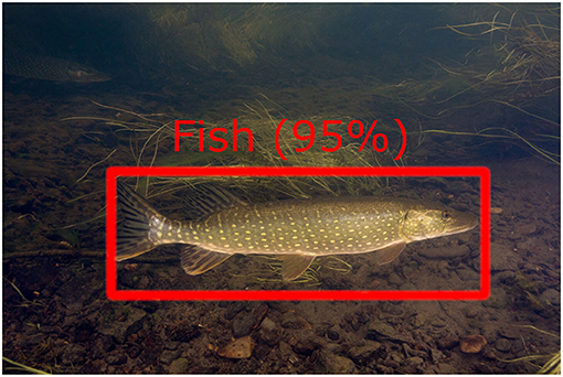
Figure 1. Example of fish detection and confidence score.

The bounding box or region mask proposed by a model may not exactly match the boundaries of an object so we need to define a similarity measure between detection regions. The intersection over union (IOU) between two detection regions (e.g., a bounding box or mask) is the area of the intersection divided by the area of the union of the predicted region and the ground-truth region. When using object detection methods we set an IOU threshold such as 0.3, 0.4, or 0.5 to determine if an object has been correctly detected or not. An overview of IOU is shown in Figure 2.

FIGURE 2

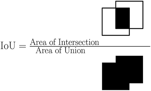
Figure 2. Overview of intersection over union.

When evaluating an image frame the proposed bounding boxes are matched to the ground truth bounding boxes. Correctly detected objects are called true positives (TP), defined as an object detected with the given IOU threshold, confidence threshold, and correct classification. Incorrectly detected objects are called false positives (FP), defined as objects detected but below the IOU threshold or with the wrong classification. Missed detections are called false negatives (FN), defined as objects with no predicted bounding box or a detection below the confidence threshold. There may be multiple or no objects in each image frame so the concept of true negatives is not typically used to evaluate multiple object detection and classification.

Precision (Equation 1) is the number of true positives divided by the sum of true positives and false positives. Detections in precise models are likely to be correct detections. Recall (Equation 2) is the number of true positives divided by the sum of true positives and false negatives. Models with high recall tend to find most objects.

$\begin{array}{ll}\text{Precision}=\frac{TP}{TP+FP}& (1)\end{array}$

$\begin{array}{ll}\text{Recall}=\frac{TP}{TP+FN}& (2)\end{array}$

There is a trade-off between these two concepts. Detections are likely to be correct from precise models at the expense of potentially missing low confidence detections. On the other hand, models with high recall tend to find most objects but may have a large number of false positives. Precision and recall may be analyzed using a precision-recall graph, with various model parameters resulting in different balances, but this can be difficult to optimize.

To optimize detection and classification models, a single metric, the average precision (AP) (Equation 3), balances both precision and recall and is based on calculating the area under a precision-recall curve. We order the ground truth objects by IOU and take a weighted sum of precision at each recall threshold with a weight based on the increase in recall. To put this another way, the average precision is the weighted sum of the precision values for the most precise detection, the two most precise detections, the three most precise detections and so on. Finally, the mean average precision (mAP) (Equation 4) is the mean of the average precision values over each classification type. Note that, despite the name, mean average precision measures both precision and recall and is the standard metric for evaluating object detection and classification models.

$\begin{array}{ll}\text{AP}={\displaystyle \sum _{k=0}^{K=n-1}}\left[\text{recall}(k)-\text{recall}(k+1)\right]*\text{precision}(k)& (3)\end{array}$

where n is the number of ground truth objects.

$\begin{array}{ll}\text{mAP}=\frac{1}{j}{\displaystyle \sum _{i=1}^j}A{P}_i& (4)\end{array}$

with AP_i being the average precision of the ith class and j the total number of classes being evaluated.

2.1.2. Evaluating Object Tracking

To evaluate the effectiveness of object tracking we need to additionally consider the duration of tracking, cases of mistaken identity and the frequency of tracking interruptions. We applied a set of criteria standardized in the CVPR19 challenge (Dendorfer et al., 2019), which are based on the CLEAR metrics proposed by Stiefelhagen et al. (2006) and track quality measures introduced by Wu and Nevatia (2006).

An object is considered mostly tracked (MT) if successfully tracked for at least 80% of frames where the object appears. An object tracked in less than 80% but at least 20% of frames is considered partially tracked (MT). Objects tracked in less than 20% of frames are called mostly lost (ML).

Identity switching (IDSW) refers to the number of times a tracked trajectory changes its matched ground-truth identity. This can occur when multiple objects are near each other and quickly change trajectories. Frequent identity switching can complicate analysis even when objects are mostly tracked.

The number of times a ground truth trajectory is interrupted is known as fragmentation. In other words, fragmentation is counted every time a trajectory status shifts from tracked to untracked, and then tracking is resumed at a later time. Fragmented detections can be unreliable.

The most widely used metric for evaluating object tracking is the multiple object tracking accuracy (MOTA). This metric considers three types of errors: false positives, missed targets, and identity switches. The formula for calculating MOTA is shown in Equation (5).

$\begin{array}{ll}{\text{MOTA}}_t=1-\frac{{\displaystyle {\sum }_t}({\text{FN}}_t+{\text{FP}}_t+{\text{IDSW}}_t)}{{\displaystyle {\sum }_t}{\text{GT}}_t}& (5)\end{array}$

where IDSW_t is the identity switches, respectively, for time t, GT_t is the number of ground truth objects, FN_t is the number of false negatives (missed targets), and FP_t the number of false positives.

2.2. Datasets

2.2.1. Dataset for Fish Detection and Classification

To evaluate our two models for fish detection and classification we used a dataset of DIDSON high resolution visual acoustic video captured from the Ocqueoc River in Michigan, USA (McCann et al., 2018b). The data in this dataset are stored in two formats: a raw acoustic format as collected from the DIDSON device and a binary format that contains images of the visualized acoustic data. We used the raw data in our analysis. Each raw video file is 30 min in duration, with 105 raw DIDSON files from 2013 and 95 from 2016. In total there are approximately 100 h of video. We extracted 524 clips with known species targets. Table 1 summarizes the number of videos for each species in this dataset. Note that the species distribution of this data is very unbalanced with up to 190 videos of the most frequent species, Lamprey, but only one video of Largemouth bass.

TABLE 1

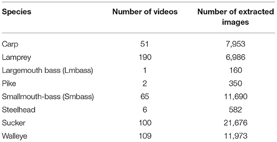
Table 1. Number of videos and extracted images of each species in the Ocqueoc River DIDSON dataset.

The Ocqueoc dataset is annotated by fisheries experts and includes spreadsheets with textual information about the position, frames, and trajectories of the identified fish species. Much of this dataset was gathered over two months in 2016 with a DIDSON visual sonar camera as well as two optical video cameras positioned to overlap the DIDSON field of view. The optical camera data was manually inspected and observed fish were cross-referenced with DIDSON data to create short videos of 5 to 20 s containing the known target. The combination of optical and sonar cameras provides high confidence species classifications on DIDSON videos.

2.2.1.1. Image Extraction

Object detection and classification models require precise labeled bounding boxes or masks which this dataset does not include. To match the requirements of our deep learning models, we converted the video files to sets of labeled images.

The raw acoustic DIDSON videos are stored in a proprietary “DDF” format. We used the DIDSON-V5 software provided by Sound Metrics to convert the DDF format files to standard AVI video files. Most videos from this dataset use a frame rate of 7 frames per second but some had lower frame rates. We extracted standardized image frames at 4 frames per second from the videos. The videos and images are annotated with the distance in meters from the DIDSON acoustic camera (see Figure 3).

FIGURE 3

Figure 3. Sample image frame captured from DIDSON visual sonar with a fish in view roughly 6 m from the camera.

2.2.1.2. Image Labeling

Training deep learning algorithms requires that, we have bounding boxes or masks that indicate the ground truth location of the objects we wish to detect. The Ocqueoc River DIDSON dataset was not annotated with bounding boxes so we used the LabelImg tool (Tzutalin, 2015) to draw bounding boxes around a subset of the images in the dataset in the YOLO format needed to train YOLO models. We prepared a small subset of labeled images for reference and then three Innovasea employees labeled a larger subset of images. Labeling images is time consuming and this step required 72 h of total labeling time. Labeling the entire dataset would take hundreds of hours. Creating custom masks would be even more labor-intensive so we reused the bounding boxes for evaluating Mask-RCNN as well by converting the YOLO format labels to the Pascal-VOC format.

One concern when training a machine learning model is “overfitting,” that is, training the model to memorize the training set rather than learning how to complete the specified task. To reduce the potential for overfitting while also generating a representative subset with different fish and conditions from this large dataset, images were only labeled every few frames (subsetting the extracted frames). This is to reduce the potential that two nearly identical images will appear in both the training and test sets.

2.2.1.3. Train and Test Sets

Following the completion of the pre-processing steps, the images containing fish have text files generated while labeling. However, there were no text files for the images that do not contain any fish. We wrote a Python script to create text files for these types of images.

After creating text files, all of these images are organized into folders based on the species. A Python script was written to extract 80% of the images randomly as the train set and 20% as the test set randomly, and then shuffled their order in these sets to reduce training bias. Table 2 shows an overview of the count of each species included in the train and test sets, which is taken into account for both the YOLOv3 and Mask-RCNN models. We also note the percentage of image frames for each species that do contain images of the fish. Note that the species distributions are very unbalanced in this dataset, ranging from only 160 total images associated with Largemouth Bass to 2741 images associated with Lamprey, which were a focus of the study that collected this data. The species distributions are somewhat similar but not exactly the same as those from the raw video data, depending on the number of videos that were labeled and the number of frames skipped by the image labelers. In addition, the percentage of images associated with each species that actually contained fish varied from 25% (Largemouth Bass) to 86.4% (Sucker) in the training set. This distribution was roughly similar in the test set. Variation in the number of fish species, biased sampling, and biased annotation can all impact the ability of a trained machine learning model to classify different species.

TABLE 2

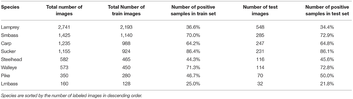
Table 2. Overview of train and test sets for training and evaluating YOLOv3 and Mask-RCNN, including the number of images for each species overall, in the training set and testing set as well as the percentage of the training and testing set images associated with those species that do contain fish.

2.2.2. Dataset for Fish Tracking

To evaluate fish tracking with Norfair we used a public dataset of optical cameras from the Wells Dam fish ladder on the Columbia River in eastern Washington state, USA (Xu and Matzner, 2018). Fish were recorded through a fish passage viewing window in the Wells Dam. These videos include Chinook, Jack Chinook, and Sockeye species. The frame rate was exactly 30 frames per second, and the video image size was exactly 1280 × 960 pixels. A total of 24,000 frames are available, with 13,405 of them containing fish. Images in this dataset are well labeled and no additional pre-processing of this data was required.

2.2.2.1. Train and Test Set

Our main goal when testing Norfair was to evaluate performance with various types of camera data recorded at various frame rates. This evaluation can help inform hardware choices and instrumentation decisions for data collection at other fish passage sites. We first split the 24,000 frames of video in the Wells Dam Camera dataset into 19,200 images for training and 4800 images for testing by randomly selecting videos to have no overlap of videos between the train and test sets.

We applied YOLOv4 and Norfair on down-sampled videos with varied frame rates per second, namely 20, 10, and 5 fps, to understand the impact of frame rate on fish tracking performance. For this evaluation, we down-sampled the training videos to 20 frames per second using a Python script, yielding 12,800 images (tracking training set 1). We then subsampled half of these images, yielding the equivalent of 6,400 images from 10 fps video (tracking training set 2). Finally, we subsampled again to obtain 3,200 images equivalent to 5 fps video (tracking training set 3).

We similarly downsampled and subsampled the test videos, resulting in three test sets with 3,200 frames of 20 fps video, 1,600 frames of 10 fps video, and 800 images of 5 fps video.

2.3. Machine Learning Models

2.3.1. YOLOv3 Detection and Classification Model

The YOLO (you only look once) family of object detection and classification models are effective models optimized for fast detections suitable for real time detection on embedded devices. We will summarize some of the features and architecture of the YOLOv3 model but see (Redmon and Farhadi, 2018) for the full details of the model. Standardized implementations and source code for YOLOv3 in the Python programming language are provided on GitHub by its creator.

The YOLOv3 architecture consists of a feature extractor and detector. The feature extractor is a 53 layer convolutional neural network called Darknet-53 which extracts features from images at three different scales suitable for large, medium and small objects relative to the image size. These features are provided to the detector network which predicts confidence values for more than 20,000 possible bounding boxes of various sizes. An algorithm called non-max suppression is applied to identify the best (if any) non-overlapping candidate object detections.

2.3.2. Mask-RCNN Detection and Classification Model

The RCNN (region-based convolutional neural network) family of object detection and classification models are an alternative architecture that can detect more general object masks than simple bounding boxes. Mask-RCNN (He et al., 2017) is the RCNN family's fourth model and an update to the previous Faster-RCNN model (Ren et al., 2015).

Mask-RCNN is divided into two stages, a backbone stage and head stage. The backbone stage uses a combination of a feature pyramid network (Lin et al., 2017) and ResNet-101 (He et al., 2016) as well as a region proposal network (Ren et al., 2015) and ROI (Region of interest) (Girshick, 2015) alignment layer for proposing regions which contains objects. The ResNet101 feature pyramid network extracts features from the raw image, analogous to the DarkNet stage of YOLOv3. Then the region proposal network applies a sliding window to these features to propose bounding box regions that may contain images. The head stage contains fully connected neural network layers which apply classification, bounding box prediction and mask prediction using the proposed object regions from the first stage.

As with YOLOv3, a standard implementation of Mask-RCNN and source code are provided by the authors in the Python programming language.

2.3.3. YOLOv4 Object Detection and Classification Model

As we discussed above, YOLOv3 contains mainly two components, a backbone feature extractor based on darknet53 and detection blocks which are used for bounding box localization and classification. YOLOv4 (Bochkovskiy et al., 2020) adds additional components for more accurate bounding box detection. It has three main stages, a feature extractor known as CSP (Cross-Stage-Partial-Connections) Darknet53 (Wang et al., 2020), a neck that connects the backbone to the head with a spatial pyramid pooling additional module (SPP) (He et al., 2015) and PANet path-aggregation-network (Liu et al., 2018), and a head that is identical to YOLOv3.

Reference implementations of YOLOv4 were not yet available when we completed the first part of this work comparing YOLOv3 to Mask-RCNN. We thus evaluated the recently released YOLOv4 only for fish tracking with Norfair.

2.4. Norfair Object Tracking Library

For fish tracking, we used the Norfair tracking library (Alori et al., 2021) in combination with YOLOv4 (Bochkovskiy et al., 2020). Norfair is a lightweight Python library for real-time object tracking that can be customized. Norfair is designed to add tracking capabilities to any object detection model using a few lines of code. Multiple new object detection models are introduced each year, as evident by the introduction of YOLOv4 during this research, so we sought a tracking method that can be applied to newer models.

For Norfair to operate, one must provide input in the form of detections made by the detector; in our case, YOLOv4 is used as the detector, which first makes detections on the images or videos and then passes those detections per frame to Norfair for object tracking.

Norfair operates by predicting each point's future location based on its previous positions and estimated velocity using a Kalman Filter. It attempts to align the previous set of locations with the detector's newly observed points using Euclidian distance or an arbitrary user-supplied distance function.

Norfair does not require training but has a number of customizable parameters that may need to be optimized for different use cases. The distance_function is the function used for calculating the distance between newly observed objects and previous detections. The distance_threshold defines the maximum distance at which a match will occur. The tracker can not fit detections or tracked items that are further away than this threshold. The tracking library maintains an initeria counter that tracks how frequently a given detection is matched to an object. The inertia counter increases with each match and decreases when there is no match. If the interia counter decreases below hit_inertia_min (default 10) then the object is no longer tracked. The inertia counter does not increase beyond hit_inertia_max (default 25) to maintain rapid responses to the disappearance of long duration tracked objects.

One final parameter is of particular interest for operating with low frame rate video. To avoid spurious detections, potential objects are followed until they have been observed for initialization_delay frames. If this parameter is too small then spurious detections will be recorded. If too large then short duration detections will be ignored.

Source code for Norfair is provided by Tryolabs in the Python programming language.

2.5. Training the Models

2.5.1. Training the YOLOv3 Model

We used convolution weights that have been pre-trained on the ImageNet (Russakovsky et al., 2015) dataset for training. The model was pre-trained on a large dataset with 80 different object classes. Applying a pre-trained model to a dataset with a different format (e.g., image dimensions, number of classification classes, etc.) requires modifying some parameters in the yolov3.config configuration file (pjreddie, 2018). yolov3.config is the file where YOLOv3 model network architecture parameters are stored.

The first change we made in the yolov3.config file was specifying the number of classes for classification which is 8 in our case. The batch value, which indicates how many images and labels are used in the forward pass to compute a gradient and update the weights via backpropagation, was set to 64. This batch value was selected according to the capacity of the NVIDIA Tesla V100 graphics processing unit (GPU) we used for training. The Subdivision parameter indicates that the batch should be divided again into blocks of images, which we set to 16. The width and height parameters, which indicate that every image will be resized to fit the network size during training and testing, are set to 608,608 which is a recommended network size for accurate detection and classification (Redmon and Farhadi, 2018). Max_batches parameters are set to (numberofclasses) × 2000, since we have 8 classes in our dataset, this was 16,000. The steps parameter should be set to 80 and 90 percent of Max_batches, so in our case, it was 12,800,14,400. The filter parameter indicates the number of output feature maps and is calculated as (classes + 5) × 3, which in our case is 39.

After the dataset and configuration file were prepared, we applied Google Colab Pro for training, using an NVIDIA Tesla V100 GPU compute processor with 16GB of RAM. The model was trained for 2,000 epochs, taking approximately 8 h.

2.5.2. Training the Mask-RCNN Model

We used convolution weights that have been pre-trained on the MS-COCO (Microsoft Common Objects in Context) (Lin et al., 2014) dataset for training. The model was pre-trained on a large dataset with about 80 different object classes, but to use it for our purposes, we need to change some parameters in the mask_rcnn.config file (cclauss, 2019).

We first set the parameter Images_per_GPU which was set to 4 based on the memory size of our GPU. The Number_of_classes parameter was set to 9 as we have 8 classes of objects in our dataset and need 1 additional class for the background. The backbone network architecture parameter was set to ResNet-101, which is the Convolutional Network architecture we utilized in the first step of Mask-RCNN. This can be chosen as either ResNet-50 or ResNet-101. We selected the larger model because it produces the best mAP when combined with Mask-RCNN according to He et al. (2017). Image_Min_Dim and Image_Max_Dim were set to 608,608.

After the dataset and configuration file were prepared, we applied Google Colab Pro for training, using an NVIDIA Tesla V100 GPU compute processor with 16GB of RAM. The model was trained for 2,000 epochs, as with YOLOv3, taking approximately 2 days.

2.5.3. Training the YOLOv4 Model (Fish Tracking)

We used convolution weights that have been pre-trained on the ImageNet dataset for training. The pretrained model was trained on a large dataset that contains about 80 classes of objects, but in order to use it for our purposes of tracking fish with Norfair, we need to change some settings in the yolov4.config configuration file (pjreddie, 2018).

The first adjustment to the yolov4.config file was the number of classes, which we set to 1 for fish tracking. In contrast to our detection and classification tests, here we only need the detector to classify objects as fish or not fish. The batch value, indicating how many images and labels are used in the forward pass to compute a gradient and update the weights via backpropagation, was set to 64 which was selected according to the capacity of the NVIDIA Tesla V100-GPU used for training. The subdivision parameter indicates that the batch should be divided again into blocks of images, and was set to 16. The width and height parameters, which indicate that every image will be resized to fit the network size during training and testing, were set to 608,608 as this is the best network size for obtaining best accuracy using YOLOv4 according to Bochkovskiy et al. (2020). Max_batches paramaters should be (numberofclasses) × 2000, so since we have 1 class in our dataset, it was set to 2000. The steps parameter should be set to 80 and 90 percent of the max batches, so in our case, we used 1600,1800. The filter parameter indicates the number of output feature maps and is calculated as (classes + 5) × 3, which in our case was 18.

Along with these settings, we applied data augmentation parameters such as hue, saturation, exposure, and random rotation, as discussed below. After the dataset and configuration file were prepared, we applied Google Colab Pro to train the model using an NVIDIA Tesla V100-GPU computing processor with 16GB of RAM. The training was conducted for 1,000 epochs after which we saved the generated model weights for testing. This took approximately 4 h.

3. Results

3.1. Fish Detection and Classification

We applied the two selected deep learning models YOLOv3 and Mask-RCNN for fish detection and classification to the Ocqueoc River DIDSON dataset. The initial results were encouraging but not sufficient for use, as is typical when applying general machine learning models to a new domain. We examined a moderate subset of the input images and fish from the test set which were not detected or were misclassified by our initial trained models, grouping them into the categories clearly visible, partially visible, and edge objects. We then applied data augmentation techniques to artificially increase the size of our dataset and enable the models to better handle detecting and classifying the fish which were not clearly visible.

3.1.1. Initial Results of YOLOv3

We evaluated the mean average precision (mAP) of YOLOv3 on the DIDSON visual acoustic data with IOU thresholds of 0.4 and 0.5. At an IOU threshold of 0.5 the model achieved an mAP of 0.29. With a less strict detection criteria, an IOU threshold of 0.4, the model achieved an mAP of 0.41. This mAP increase suggests that the model may be detecting the general vicinity of the fish but is not finding their position accurately.

We also examined individual performance of YOLOv3 on each species in the dataset (Table 3). This analysis includes the number of true and false positives as well as the average precision for each species with IOU detection thresholds of 0.4 and 0.5. In general, we observed the worst performance in species with the least training samples (Largemouth Bass IOU = 0.4,AP = 0, 160 images and Steelhead IOU = 0.4,AP = 0.28, 582 images). However, the model performed poorly on some species with a large number of training samples (Lamprey IOU = 0.4,AP = 0.36, 2,741 images) and the model performed well on some species with a small number of training samples (Walleye IOU = 0.4, AP = 0.7, 573 images). Fish shape as well as the relative number of training images which actually contain fish (e.g., Lamprey with only a 36.6% rate of positive samples) may be contributing factors to these results.

TABLE 3

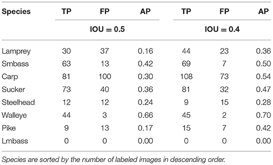
Table 3. Results of the YOLOv3 model on each species in the Ocqueoc River DIDSON dataset with IOU thresholds of 0.4 and 0.5.

3.1.2. Initial Results of Mask-RCNN

We also evaluated the mean average precision (mAP) of Mask-RCNN on the DIDSON visual acoustic data with IOU thresholds of 0.4 and 0.5. At an IOU threshold of 0.5 the model achieved an mAP of 0.18. The mAP with an IOU threshold of 0.4 was 0.32. As with YOLOv3, This mAP increase suggests that the model may be detecting the general vicinity of the fish but is not finding their position accurately. Moreover, Mask-RCNN performed worse than YOLOv3 on average for this dataset.

We also examined individual performance of Mask-RCNN on each species in the dataset (Table 4). This analysis includes the number of true and false positives as well as the average precision for each species with IOU detection thresholds of 0.4 and 0.5. We saw similar patterns as with YOLOv3, namely that species with few samples were difficult to detect and classify. Mask-RCNN performed slightly better than YOLOv3 with some species, including Carp, Largemouth Bass, and Pike. However, Mask-RCNN performed the same or worse as YOLOv3 at detecting and classifying most of the species, particularly Lamprey (AP = 0.06).

TABLE 4

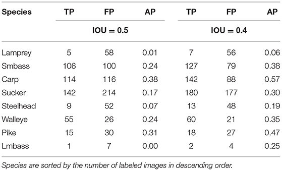
Table 4. Results of the Mask-RCNN model on each species in the Ocqueoc River DIDSON dataset with IOU thresholds of 0.4 and 0.5.

3.1.3. Evaluation of Difficult Cases

The initial overall performance of both YOLOv3 and MASK-RCNN models on our dataset was not particularly impressive. To understand this failure, we randomly selected 1,000 images from the test set to evaluate more closely. Our initial trained YOLOv3 and Mask-RCNN models were tested on these 1,000 images with an IOU threshold of 0.5. The 804 images which contained objects not detected at an IOU threshold of 0.5 were then run with IOU thresholds 0.1, 0.2, 0.3, and 0.4. Upon examination we categorized these images into three categories, that is, containing fish that were clearly visible (Figure 4), edge objects (Figure 5), or partially visible (Figure 6). In total there were 58 clearly visible images, 702 partially visible images, and 44 edge object images.

FIGURE 4

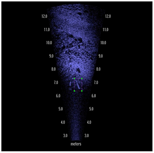
Figure 4. Example image where the fish is clearly visible from DIDSON visual sonar.

FIGURE 5

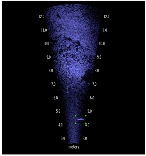
Figure 5. Example image where the fish is at the edge of the DIDSON visual sonar image.

FIGURE 6

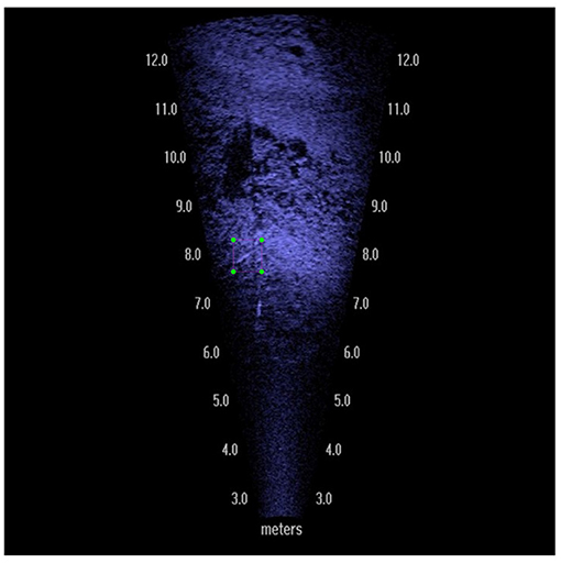
Figure 6. Example image where the fish is partially visible.

We observed that most failures were a result of partially visible objects. With partial visibility, the machine learning models often detected the fish at low IOU values with bounding boxes near but very different dimensions than our labeled ground truth boxes (Figure 7).

FIGURE 7

Figure 7. Example image where a partially visible fish is detected with an IOU of 0.3, below the threshold. The green box indicates the labeled ground truth and the red box indicates the bounding box predicted by YOLOv3.

3.1.4. Image Augmentation

At this stage, we hypothesized that our models were suffering from a combination of insufficient training examples and partially visible training examples. One of the best techniques for improving model performance in these conditions is to apply image augmentation techniques. Image augmentation modifies the test set images in various ways, generating additional training examples. The specific image augmentation techniques chosen can help the models better generalize and handle challenging conditions. We selected image-based transformations to help teach the model to identify fish at different orientations and in darker regions of the visual sonar-based images. Modern machine learning models like YOLOv3 and Mask-RCNN can integrate several different common augmentations which must be selected based on the dataset. Selecting inappropriate augmentations can increase training time and even reduce accuracy.

In particular, we applied saturation, contrast, hue, and rotation augmentations. Every augmentation was applied during training to each training image with random variation based the following parameters. The number of training samples per epoch was the same without and with augmentation.

Saturation modifies the color intensity. Larger values apply greater variance. We used a saturation range of [0 to 1.5], which is applied randomly to images when training the model.

Exposure determines the amount of black or white that is added to colors. The higher the value, the greater the variance, possibly making it appear as if the images were over-or under-exposed. We applied an exposure range of [0 to 1.5].

Hue Hue can be thought of as the “shade” of the colors in an image. We applied a Hue range of [0 to 0.5]. The Hue augmentation changes the color channels of an input image at random, causing a model to explore several color schemes for objects and scenes in the image. This strategy is important for ensuring that a model does not memorize the colors of a given object or scene.

Random Rotation changes the angle of objects present in the images. Objects can be skewed in either direction. We applied a rotation range of [–90 to 90 degrees]. Rotation augmentations may help the models learn to detect fish at different angles or partially visible and may also reduce reliance on the boundary shape of the DIDSON images.

Note that although DIDSON images are a representation of sensor return values and, therefore, do not contain color information naturally, the images as presented to YOLOv3 and Mask-RCNN are color images and the models benefit from additional modified training examples which enable them to learn to use more robust information from the images.

3.1.5. Final Results of YOLOv3

Applying image augmentation during training greatly improved the results of YOLOv3 on the Ocqueoc River DIDSON dataset. The results with an IOU threshold of 0.5 improved from 0.29 mAP to 0.59 mAP. The results with an IOU threshold of 0.4 improved from 0.41 mAP to 0.73 mAP.

The per-species detection and classification results were similarly improved (Table 5). We can see that YOLOv3 had a higher average precision on Walleye with an IOU threshold of 0.5, yet achieved a higher average precision for Smallmouth bass with an IOU threshold of 0.4, demonstrating that model detection performance varies with IOU. We also observe that the number of false positive values for each species is higher for an IOU threshold of 0.5 than for 0.4, demonstrating that the YOLOv3 model prediction of bounding box changes as the IOU value increases. Most encouraging was that the average precision on Largemouth Bass increased from 0 to 0.56 with an IOU threshold of 0.5, demonstrating that increasing the number of training images allows us to detect and classify some species of fish even with few training samples.

TABLE 5

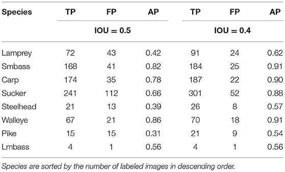
Table 5. Results of the YOLOv3 model with image augmentation on each species in the Ocqueoc River DIDSON dataset with IOU thresholds of 0.4 and 0.5.

3.1.6. Final Results of Mask-RCNN

Applying image augmentation during training also improved the results of MASK-RCNN on the Ocqueoc River DIDSON dataset. The results with an IOU threshold of 0.5 improved from 0.18 mAP to 0.54 mAP. The results with an IOU threshold of 0.4 improved from 0.32 mAP to 0.62 mAP.

As with YOLOV3, the per-species detection and classification results with MASK-RCNN were greatly improved (Table 6).

TABLE 6

Table 6. Results of the MASK-RCNN model with image augmentation on each species in the Ocqueoc River DIDSON dataset with IOU thresholds of 0.4 and 0.5.

3.1.7. Fish Detection and Classification Results

The highest mAP achieved by YOLOv3 and Mask-RCNN was 0.73 and 0.62, respectively. These results demonstrate that it is feasible to detect and classify fish species using visual acoustic data from high resolution acoustic cameras like the DIDSON devices deployed on the Ocqueoc River. YOLOv3 achieved a higher mAP in our dataset and with our chosen parameters, suggesting that YOLO models may perform better on this task. As a result, we focused on the newly introduced YOLOv4 for our later tests on fish tracking with Norfair. In addition, the processing rate of video frames was faster with YOLOv3 (24 fps) than with Mask-RCNN (8 fps).

We also observed that these detection and classification models can achieve good average precision on species when supplied with ample training examples such as in this dataset with Carp, Smallmouth Bass and Walleye when compared to species with fewer images such as Largemouth Bass, Pike, and Steelhead. Sufficient training examples will need to be collected to use these models on rare fish, although image augmentation techniques can reduce the number of training examples needed.

4. Fish Tracking

We combined YOLOv4 with Norfair for fish tracking. We trained three different YOLOv4 models, one on each of our subsampled training sets designed to mimic video at 20, 10, and 5 fps. We evaluated the performance of fish tracking (Table 7) including the overall duration of tracking, number of false positives and negatives, ID switches, fragmentation and multiple object tracking accuracy. Note that these results report tracking duration for each detected class and, thus, for all fish combined in this dataset.

TABLE 7

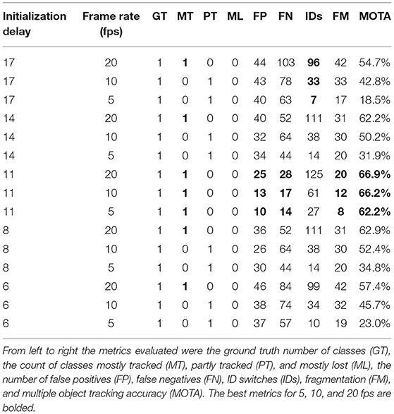
Table 7. Norfair fish tracking results on video with 5, 10, and 20 fps, using initialization delays ranging from 6–17.

In general, fish were more difficult to track on the low frame rate data as evidence by the low MOTA values. Note that the low frame rate data naturally contains 1/4 of the frames of video and so has relatively high levels of false positives, false negatives and fragmentation. As such, one must be careful when comparing fish tracking performance between videos with different frame rates.

The greatest MOTA attained by Norfair was 66.9% for 20 fps videos, 66.2% for 10 fps videos, and 62.2% for 5 fps videos, all at an initialization delay of 11. In general the best performance on all metrics except ID switches was obtained with an initialization delay of 11. The lower rate of ID switches at very small and very large initialization delays is likely caused by the large number of false positives at those initialization delays, suggesting that this metric needs to be considered with the context of other metrics.

Figure 8 shows a comparison of MOTA of Norfair at various frame rates. The MOTA of Norfair was highest at an initialization delay of 11, and as the initialization delay is reduced, the MOTA value decreases. MOTA values decline as fps decreases and, for all values of initialization delay, the highest MOTA is achieved for videos of 20 fps and the lowest with videos of 5 fps. We can conclude from these results that Norfair tracks fish relatively well on videos with high frame rates but poorly on low frame rate video with the default initialization delay settings of 17. Tuning the initialization delay parameter allows Norfair to also track fish in low frame rate video with similar performance to high frame rate video.

FIGURE 8

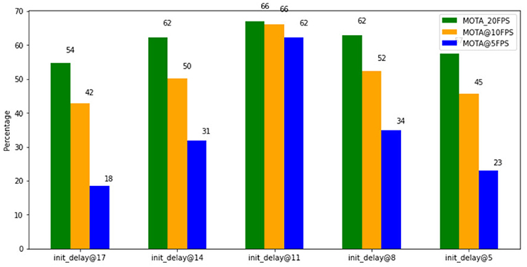
Figure 8. Comparison of MOTA of Norfair at different Intialization_delay values.

5. Discussion

The main aim of this research was to evaluate the performance of state of the art deep learning models on visual acoustic data and video camera data for detection, classification, and tracking fish. We first tested the feasibility of using deep learning for detection and classification on eight distinct species of fish captured by a high-resolution DIDSON imaging sonar in the Ocqueoc River. The dataset contains metadata observations indicating which videos and frames contained fish, their species, and text descriptions of their approximate location which were later converted into images for performing detection and classification tasks using YOLOv3 and Mask-RCNN models. To evaluate fish tracking, we used a dataset containing underwater optical videos recorded from the Wells Dam fish ladder on the Columbia River in Washington State, USA. This dataset contains images of fish which were input to a YOLOv4 model for integration with the Norfair algorithm for performing fish tracking.

The maximum mean average precision achieved by YOLOv3 for fish classification and detection was 0.73 with an IOU threshold of 0.4. In contrast, Mask-RCNN achieved 0.62 mAP at this IOU threshold. In general, our results show that we can indeed detect and classify fish by species using DIDSON imaging sonar with these deep learning models. YOLOv3 achieved a higher mAP when compared to Mask-RCNN, as well as higher AP for individual species, suggesting that YOLOv3 may be a better model to deploy for real-time fish detection and classification when using acoustic data. Moreover, YOLOv3 was faster in terms of processing image frames per second with a rate of 24 fps in comparison to the 8 fps of Mask-RCNN. As such, YOLO family models are recommended for deployment on embedded devices requiring real-time processing.

Infrequently sampled fish were difficult to classify so we recommend having at least 400 training examples for each species of fish to obtain accurate species classifications. More training instances may be needed if attempting to classify very similar species of fish or much larger sets of species than the eight we classified here. Image augmentation techniques including saturation, exposure, hue, and random rotation were needed to achieve reasonable average precision values on visual acoustic data and with unbalanced species distributions. In general, an evaluation of difficult classification cases and optimization techniques like image augmentation are needed to achieve useful performance when attempting to apply a general purpose machine learning model to a new domain or type of data.

After evaluating models for detecting and classifying fish species, we briefly investigated the task of tracking and counting fish. For this purpose, we integrated the recently released YOLOv4 model with the Norfair tracking library. Different deployments often use different video equipment or settings to save money, power and storage. In particular, organizations may have large historical collections of low frame rate video captured from older equipment that requires automated analysis. As such we downsampled videos of fish to obtain equivalent videos at different frame rates. We explored varying the Norfair initialization delay parameter, which controls the number of detections of an object required to begin tracking, as a method to optimize tracking performance on low frame rate video. The greatest MOTA attained by Norfair was 66.9% for 20 fps videos, 66.2% for 10 fps videos, and 62.2% for 5 fps videos at an initialization delay of 11. Our results were much worse at lower and higher initialization delay values, including the default parameter of 17. Our results suggest that YOLOv4 plus Norfair has promise for fish tracking and that tuning the initialization delay can recover performance on low frame rate video.

5.1. Limitations

• Image labeling is a slow error-prone task but large amounts of labeled data are needed to train accurate and robust supervised models like the type of models we evaluated here. We only labeled a subset of the Ocqueoc River DIDSON dataset in our tests and it would take a large amount of effort to label the entire dataset manually. Moreover, inaccurate labels may reduce the performance of deep learning models.

• Although we were able to achieve good classification performance on visual acoustic images, we observed that this is a challenging task. Fish are not always clearly visible in the images and there is a lot of background noise, so one should expect lower average precision than can be obtained from optical cameras. However, this tradeoff may be worth pursuing because acoustic sensors and cameras can be used in low light or deep water.

• We were only able to perform limited testing of fish tracking on the public datasets available to us. In particular, we observed a number of identity switches which may make it difficult to accurately count fish or, in particular, analyze their trajectories. Moreover, there are a large number of metrics needed to evaluate fish tracking and it remains unclear how to thoroughly compare performance between videos captured with different frame rates.

5.2. Future Work

• Human annotation has long been recognized as a limiting factor to design, training and testing of deep learning models. Newer self-supervised vision transformer models such as the recent DINO (Distillation with no labels) (Caron et al., 2021) model from Facebook might help reduce this limiting factor. Self-supervised models learn a representation of images or other data that can be applied to training models with fewer (or no?) labeled training samples. Reducing or automating the work of labeling datasets for deep learning would greatly expand the use and availability of deep learning models for specialized domains such as fish classification.

• We observed that image clarity of DIDSON sonar images had a direct impact on performance of deep learning models for fish detection and species classification We applied several augmentation methods which greatly improved performance. Developing and testing new augmentation methods purpose built for acoustic data could improve performance and reduce the number of training samples needed. Similarly, other computer vision techniques could enhance the images before processing and improve performance.

• Automatic tuning strategies could reduce or eliminate the requirement to manually tune tracking parameters such as the Norfair initialization delay parameter. Moreover, we tested only a small subset of the possible models for detection, classification and tracking and many more deep learning models are introduced every year. Our goal here was simply evaluating the feasibility of these techniques so we do not claim that the models tried here are necessarily optimal. Thus, we recommend evaluating other models and on larger datasets to obtain a better understanding of how deep learning can be applied to the tasks of detecting, classifying, and tracking fish.

In summary, we demonstrated that deep learning models are now a viable approach for detecting and classifying fish using visual acoustic data. Challenges remain to be solved including reducing or sidestepping the time and effort needed to label large high quality datasets. We found that data augmentation strategies play a key role in improving the models detection and classification performance by increasing the number of training samples and teaching the model to handle more challenging partially visible fish. The Norfair library worked well for tracking fish on video camera data, and tweaking the initialization delay parameter allowed us to apply Norfair to track fish in low frame rate video.

Data Availability Statement

Publicly available datasets were analyzed in this study. This data can be found at: McCann et al. (2018a) and EyeSea (2018).

Author Contributions

VK wrote the data processing code, labeled the initial subset of the Ocqueoc River DIDSON dataset, conducted the experiments, conducted the analysis, and created the figures. CW wrote the first draft of the manuscript, based on VK's thesis. All authors contributed to manuscript revision, read and approved the submitted version, and conception and design of the study.

Funding

This research was supported by the Mitacs Accelerate Program (IT22090) with joint funding from Mitacs and Innovasea. Computations were performed on Google Colab Pro and the DeepSense high-performance computing platform. Publication costs were supported by Innovasea and DeepSense. The work of LT was undertaken, in part, thanks to funding from the Canada Research Chairs program and NSERC.

Conflict of Interest

MR, FS, and JQ were employed by the company Innovasea. VK conducted this research while a student at Dalhousie University but was employed by Innovasea after graduation. No offer of employment, express or implied, was made conditional on any outcomes of this research. The authors declare that this study received funding from the Mitacs Accelerate program with co-funding provided by Innovasea. Innovasea was involved in the study as described in the Author Contributions and Acknowledgments.

The remaining authors declare that this research was conducted in the absence of any commercial or financial relationships that could be construed as a potential conflict of interest.

Publisher's Note

All claims expressed in this article are solely those of the authors and do not necessarily represent those of their affiliated organizations, or those of the publisher, the editors and the reviewers. Any product that may be evaluated in this article, or claim that may be made by its manufacturer, is not guaranteed or endorsed by the publisher.

Acknowledgments

We wish to thank Innovasea staff Aubrey Ingraham, Jeff Garagan, and Tim Hatt for labeling the larger subset of the Ocequeoc River DIDSON dataset. We also want to acknowledge the support of DeepSense staff Jason Newport, Lu Yang, Geetika Bhatia and Mahbubur Rahman who contributed suggestions and computing support. This work is based on VK's thesis Kandimalla (2021).

References

Agarwal, V. K., Sivakumaran, N., and Naidu, V. (2016). Six object tracking algorithms: a comparative study. Indian J. Sci. Technol. 9, 1–9. doi: 10.17485/ijst/2016/v9i30/99017

PubMed Abstract | CrossRef Full Text | Google Scholar

Ali-Gombe, A., Elyan, E., and Jayne, C. (2017). “Fish classification in context of noisy images,” in International Conference on Engineering Applications of Neural Networks (Athens: Springer), 216–226.

Google Scholar

Alori, J., Descoins, A., Ríos, B., and Castro, A. (2021). tryolabs/norfair: v0.3.1. doi: 10.5281/zenodo.5146254

CrossRef Full Text

Bathija, A., and Sharma, G. (2019). Visual object detection and tracking using yolo and sort. Int. J. Eng. Res. Technol. 8, 705–708.

PubMed Abstract | Google Scholar

Bewley, A., Ge, Z., Ott, L., Ramos, F., and Upcroft, B. (2016). “Simple online and realtime tracking,” in 2016 IEEE international conference on image processing (ICIP) (Phoenix, AZ: IEEE), 3464–3468.

Google Scholar

Blemel, H., Bennett, A., Hughes, S., Wienhold, K., Flanigan, T., Lutcavage, M., et al. (2019). Improved fish tagging technology: field test results and analysis. in OCEANS 2019-Marseille (Marseille: IEEE), 1–6.

Google Scholar

Bochkovskiy, A., Wang, C.-Y., and Liao, H.-Y. M. (2020). YOLOv4: optimal speed and accuracy of object detection. arXiv preprint arXiv:2004.10934.

PubMed Abstract | Google Scholar

Capoccioni, F., Leone, C., Pulcini, D., Cecchetti, M., Rossi, A., and Ciccotti, E. (2019). Fish movements and schooling behavior across the tidal channel in a mediterranean coastal lagoon: an automated approach using acoustic imaging. Fish. Res. 219, 105318. doi: 10.1016/j.fishres.2019.105318

CrossRef Full Text | Google Scholar

Caron, M., Touvron, H., Misra, I., Jégou, H., Mairal, J., Bojanowski, P., et al. (2021). “Emerging properties in self-supervised vision transformers,” in Proceedings of the IEEE/CVF International Conference on Computer Vision (ICCV), 9650–9660.

Google Scholar

cclauss (2019). Mask_RCNN. Available online at: https://github.com/matterport/Mask_RCNN/

Dendorfer, P., Rezatofighi, H., Milan, A., Shi, J., Cremers, D., Reid, I., et al. (2019). CVPR19 tracking and detection challenge: how crowded can it get? arXiv preprint arXiv:1906.04567.

Google Scholar

EyeSea (2018). DataHub. Available online at: https://data.pnnl.gov/group/nodes/dataset/12978

Girshick, R. (2015). “Fast R-CNN,” in Proceedings of the IEEE International Conference on Computer Vision (Santiago, CH: IEEE), 1440–1448.

He, K., Gkioxari, G., Dollár, P., and Girshick, R. (2017). “Mask R-CNN,” in Proceedings of the IEEE International Conference on Computer Vision (Venice: IEEE), 2961–2969.

Google Scholar

He, K., Zhang, X., Ren, S., and Sun, J. (2015). Spatial pyramid pooling in deep convolutional networks for visual recognition. IEEE Trans. Pattern Anal. Mach. Intell. 37, 1904–1916. doi: 10.1109/TPAMI.2015.2389824

PubMed Abstract | CrossRef Full Text | Google Scholar

He, K., Zhang, X., Ren, S., and Sun, J. (2016). “Deep residual learning for image recognition,” in Proceedings of the IEEE Conference on Computer Vision and Pattern Recognition (Las Vegas, NV: IEEE), 770–7.

PubMed Abstract | Google Scholar

Held, D., Thrun, S., and Savarese, S. (2016). “Learning to track at 100 fps with deep regression networks,” in European Conference on Computer Vision (Amsterdam: Springer), 749–765.

Google Scholar

Hilborn, R., Amoroso, R. O., Anderson, C. M., Baum, J. K., Branch, T. A., Costello, C., et al. (2020). Effective fisheries management instrumental in improving fish stock status. Proc. Natl. Acad. Sci. U.S.A. 117, 2218–2224. doi: 10.1073/pnas.1909726116

PubMed Abstract | CrossRef Full Text | Google Scholar

Jalal, A., Salman, A., Mian, A., Shortis, M., and Shafait, F. (2020). Fish detection and species classification in underwater environments using deep learning with temporal information. Ecol. Inform. 57, 101088. doi: 10.1016/j.ecoinf.2020.101088

CrossRef Full Text | Google Scholar

Kandimalla, V. (2021). Deep Learning Approaches To Classify and Track at-Risk Fish Species (Master's thesis), Dalhousie University, Halifax, NS, Canada.

Google Scholar

Kuhn, H. W. (1955). The Hungarian method for the assignment problem. Naval Res. Logist. Quart. 2, 83–97. doi: 10.1002/nav.3800020109

PubMed Abstract | CrossRef Full Text | Google Scholar

LeCun, Y., Bengio, Y., and Hinton, G. (2015). Deep learning. Nature 521, 436–444. doi: 10.1038/nature14539

PubMed Abstract | CrossRef Full Text | Google Scholar

Li, L., Danner, T., Eickholt, J., McCann, E., Pangle, K., and Johnson, N. (2017). “A distributed pipeline for didson data processing,” in 2017 IEEE International Conference on Big Data (Big Data) (Boston, MA: IEEE), 4301–4306.

Google Scholar

Lin, T.-Y., Dollár, P., Girshick, R., He, K., Hariharan, B., and Belongie, S. (2017). “Feature pyramid networks for object detection,” in Proceedings of the IEEE Conference on Computer Vision and Pattern Recognition (Honolulu, HI), 2117–2125.

Google Scholar

Lin, T.-Y., Maire, M., Belongie, S., Hays, J., Perona, P., Ramanan, D., et al. (2014). “Microsoft COCO: common objects in context,” in European Conference on Computer Vision (Zürich: Springer), 740–755.

Google Scholar

Liu, S., Qi, L., Qin, H., Shi, J., and Jia, J. (2018). “Path aggregation network for instance segmentation,” in Proceedings of the IEEE Conference on Computer Vision and Pattern Recognition (Salt Lake City, UT), 8759–8768.

Google Scholar

Martignac, F., Daroux, A., Bagliniere, J.-L., Ombredane, D., and Guillard, J. (2015). The use of acoustic cameras in shallow waters: new hydroacoustic tools for monitoring migratory fish population. a review of didson technology. Fish Fish. 16, 486–510. doi: 10.1111/faf.12071

CrossRef Full Text | Google Scholar

McCann, E., Li, L., Pangle, K., Johnson, N., and Eickholt, J. (2018a). FigShare. Available online at: https://doi.org/10.6084/m9.figshare.c.4039202

McCann, E., Li, L., Pangle, K., Johnson, N., and Eickholt, J. (2018b). An underwater observation dataset for fish classification and fishery assessment. Sci. Data 5, 1–8. doi: 10.1038/sdata.2018.190

PubMed Abstract | CrossRef Full Text | Google Scholar

Moursund, R. A., Carlson, T. J., and Peters, R. D. (2003). A fisheries application of a dual-frequency identification sonar acoustic camera. ICES J. Mar. Sci. 60, 678–683. doi: 10.1016/S1054-3139(03)00036-5

CrossRef Full Text | Google Scholar

Ning, G., Zhang, Z., Huang, C., Ren, X., Wang, H., Cai, C., and He, Z. (2017). Spatially supervised recurrent convolutional neural networks for visual object tracking. In 2017 IEEE International Symposium on Circuits and Systems (ISCAS) (Baltimore, MD: IEEE), 1–4.

Google Scholar

Padilla, R., Netto, S. L., and da Silva, E. A. (2020). “A survey on performance metrics for object-detection algorithms,” in 2020 International Conference on Systems, Signals and Image Processing (IWSSIP) (Niterói: IEEE), 237–242.

Google Scholar

Pengying, T., Pedersen, M., Hardeberg, J. Y., and Museth, J. (2019). “Underwater fish classification of trout and grayling,” in 2019 15th International Conference on Signal-Image Technology & Internet-Based Systems (SITIS) (Sorrento: IEEE), 268–273.

Google Scholar

pjreddie (2018). Darknet. Available Online at: https://github.com/pjreddie/darknet/blob/master/cfg/yolov3.cfg/

Rathi, D., Jain, S., and Indu, S. (2017). “Underwater fish species classification using convolutional neural network and deep learning,” in 2017 Ninth International Conference on Advances in Pattern Recognition (ICAPR) (Bengaluru: IEEE), 1–6.

Google Scholar

Redmon, J., Divvala, S., Girshick, R., and Farhadi, A. (2016). “You only look once: Unified, real-time object detection,” in Proceedings of the IEEE Conference on Computer Vision and Pattern Recognition (Las Vegas, NV), 779–788.

Google Scholar

Redmon, J., and Farhadi, A. (2018). YOLOv3: an incremental improvement. arXiv preprint arXiv:1804.02767.

Google Scholar

Ren, S., He, K., Girshick, R., and Sun, J. (2015). Faster r-cnn: towards real-time object detection with region proposal networks. Adv. Neural Inf. Process. Syst. 28, 91–99. doi: 10.1109/TPAMI.2016.2577031

PubMed Abstract | CrossRef Full Text | Google Scholar

Russakovsky, O., Deng, J., Su, H., Krause, J., Satheesh, S., Ma, S., et al. (2015). Imagenet large scale visual recognition challenge. Int. J. Comput. Vis. 115, 211–252. doi: 10.1007/s11263-015-0816-y

CrossRef Full Text | Google Scholar

Spampinato, C., Giordano, D., Di Salvo, R., Chen-Burger, Y.-H. J., Fisher, R. B., and Nadarajan, G. (2010). “Automatic fish classification for underwater species behavior understanding,” in Proceedings of the First ACM International Workshop on Analysis and Retrieval of Tracked Events and Motion in Imagery Streams (Firenze), 45–50.

Google Scholar

Spampinato, C., Palazzo, S., Giordano, D., Kavasidis, I., Lin, F.-P., and Lin, Y.-T. (2012). “Covariance based fish tracking in real-life underwater environment,” in VISAPP (2) (Rome), 409–414.

Google Scholar

Stiefelhagen, R., Bernardin, K., Bowers, R., Garofolo, J., Mostefa, D., and Soundararajan, P. (2006). “The clear 2006 evaluation,” in International Evaluation Workshop on Classification of Events, Activities and Relationships (Southampton: Springer), 1–44.

Google Scholar

Sung, M., Yu, S.-C., and Girdhar, Y. (2017). “Vision based real-time fish detection using convolutional neural network,” in OCEANS 2017-Aberdeen (Aberdeen: IEEE), 1–6.

PubMed Abstract | Google Scholar

Terayama, K., Shin, K., Mizuno, K., and Tsuda, K. (2019). Integration of sonar and optical camera images using deep neural network for fish monitoring. Aquacult. Eng. 86:102000. doi: 10.1016/j.aquaeng.2019.102000

CrossRef Full Text | Google Scholar

Tseng, C.-H., and Kuo, Y.-F. (2020). Detecting and counting harvested fish and identifying fish types in electronic monitoring system videos using deep convolutional neural networks. ICES J. Mar. Sci. 77, 1367–1378. doi: 10.1093/icesjms/fsaa076

CrossRef Full Text | Google Scholar

Tušer, M., Frouzová, J., Balk, H., Muška, M., Mrkvička, T., and Kubečka, J. (2014). Evaluation of potential bias in observing fish with a didson acoustic camera. Fish. Res. 155, 114–121. doi: 10.1016/j.fishres.2014.02.031

CrossRef Full Text | Google Scholar

Tzutalin (2015). Labelimg. Available online at: https://github.com/tzutalin/labelImg

Vianna, G. M., Zeller, D., and Pauly, D. (2020). Fisheries and policy implications for human nutrition. Curr. Environ. Health Rep. 7, 1–9. doi: 10.1007/s40572-020-00286-1

PubMed Abstract | CrossRef Full Text | Google Scholar

Villon, S., Mouillot, D., Chaumont, M., Darling, E. S., Subsol, G., Claverie, T., et al. (2018). A deep learning method for accurate and fast identification of coral reef fishes in underwater images. Ecol. Inform. 48, 238–244. doi: 10.1016/j.ecoinf.2018.09.007

CrossRef Full Text | Google Scholar

Wang, C.-Y., Liao, H.-Y. M., Wu, Y.-H., Chen, P.-Y., Hsieh, J.-W., and Yeh, I.-H. (2020). “CSPNet: a new backbone that can enhance learning capability of CNN,” in Proceedings of the IEEE/CVF Conference on Computer Vision and Pattern Recognition Workshops (Seattle, WA), 390–391.

Google Scholar

Wojke, N., Bewley, A., and Paulus, D. (2017). “Simple online and realtime tracking with a deep association metric,” in 2017 IEEE International Conference on Image Processing (ICIP) (Beijing: IEEE), 3645–3649.

Google Scholar

Wu, B., and Nevatia, R. (2006). “Tracking of multiple, partially occluded humans based on static body part detection,” in 2006 IEEE Computer Society Conference on Computer Vision and Pattern Recognition (CVPR'06), Vol. 1, (New York, NY: IEEE), 951–958.

Google Scholar

Xu, W., and Matzner, S. (2018). “Underwater fish detection using deep learning for water power applications,” in 2018 International Conference on Computational Science and Computational Intelligence (Las Vegas, NV: IEEE), 313–318.

Google Scholar