A hyperspectral image reconstruction algorithm based on RGB image using multi-scale atrous residual convolution network

1. Introduction

RGB image is a color image composed of red, green and blue channels. Hyperspectral image is an image composed of dozens or hundreds of channels, which is divided in detail in the dimension of spectrum, as shown in Figure 1A. Hyperspectral images not only contain image information, but also can be expanded in the spectral dimension. For a certain substance, different spectral wavelengths may correspond to different values, and the spectral curve of the substance can be obtained, as shown in Figure 1B. Therefore, hyperspectral images provide richer spectral information than RGB images. Targets with different components and attributes may have similar appearances, but their spectral curves will be quite distinct. This means hyperspectral images have unique advantages in computer vision tasks such as target recognition and image analysis, leading to the gradual application of hyperspectral image analysis in various research fields such as remote sensing, agriculture, medicine and ocean sciences. For the latter, hyperspectral data have been used in the monitoring of marine water quality (such as total suspended solids, chlorophyll, dissolved organic matter, etc.) (Veronez et al., 2018; Peterson et al., 2020; Ying et al., 2021) and marine disasters (such as red tide, oil spills, etc.) (Guga, 2020; Qizhong et al., 2021).

FIGURE 1

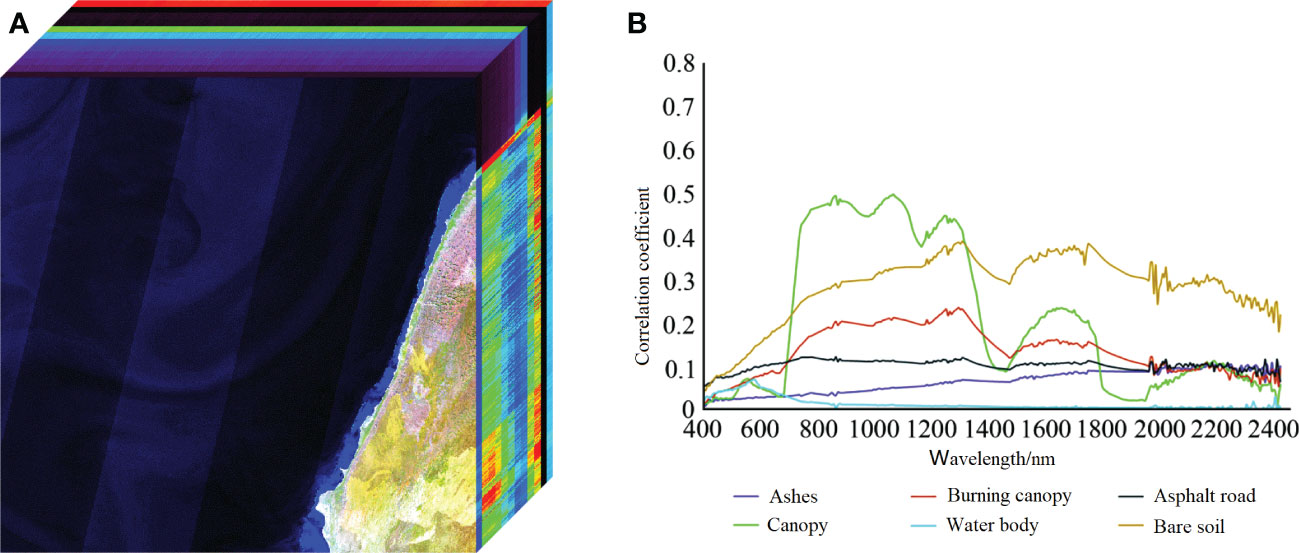
Figure 1 Hyperspectral 3D data from the Sentinel-2 satellite along the northern coast of Australia, (A) UTM zone 49S, (B) Spectral curves of different substances.

However, hyperspectral images also bring significant capture complexity, high costs (Geelen et al., 2014; Beletkaia and Pozo, 2020), or high light field requirements (Descour and Dereniak, 1995). As a result, reconstructing hyperspectral images from ubiquitous RGB images at a low cost has become a hot research topic. There is a complex correlation between the pixel values of RGB images and hyperspectral images. However, compared with hyperspectral images, RGB images provide less spectral information, which makes it very difficult to reconstruct hyperspectral images from RGB images. Therefore, reconstructing hyperspectral images from RGB images is a very challenging task.

The existing methods of reconstructing hyperspectral images from RGB images can be roughly divided into two categories: the first is to design specific systems based on ordinary RGB cameras. Goel (Goel et al., 2015) designed a hyperspectral camera using time-division multiplexing illumination source to realize reconstruction, which is a universal hyperspectral imaging system for visible light and NIR wavelength. The camera has a frame rate of 150 FPS and a maximum resolution of 1280 × 1024. Wug (Oh et al., 2016) used multiple color cameras for reconstruction, and used different spectral sensitivities of different camera sensors to reconstruct the hyperspectral images, with a resolution of 200x300 and an imaging time of 2 minutes. However, these methods rely on strict environmental conditions or additional equipment. The second method is to directly model the mapping relationship between RGB images and hyperspectral images of ordinary cameras by using the correlation and a large volume of training data. Because this mapping is highly nonlinear, machine learning methods are usually employed.

Some early work (Farnaz et al., 2008; Arad and Benshahar, 2016) expressed this problem as a weighted combination of basis functions, using principal component analysis to extract the basis function from hyperspectral data sets. Other studies use sparse coding to reconstruct hyperspectral data from RGB images (Antonio, 2015; Jia et al., 2017; Aeschbacher et al., 2017). Nguyen et al. (2014) proposed to use radial basis function networks to learn the mapping from RGB image to hyperspectral image, reduce the impact of illumination on network performance, and do white balance processing on the input image. Arad et al. (Antonio, 2015) constructed a new hyperspectral dataset of natural scenes and used it to build a sparse spectral dictionary and its corresponding RGB projection to reconstruct hyperspectral images from RGB images.

Recently, a number of studies have explored end-to-end mapping of the relationship between RGB images and hyperspectral images through neural networks (Shoeiby et al., 2018a; Shoeiby et al., 2018b; Kaya et al., 2019). Galliani, Alvarez Gila, Liu et al. (Galliani et al., 2017; Alvarezgila et al., 2017; Pengfei et al., 2020) applied convolutional neural network and GAN to hyperspectral image reconstruction. By using multi-scale feature pyramid module in GAN, the correlation between local and global features is established. Good reconstruction results have been achieved. Xiong et al. (2017) proposed an HSCNN network for reconstructing hyperspectral images from RGB images and compressed measurements. In order to simplify the sampling process. – proposed an HSCNN-D network, which achieved good reconstruction results. proposed a novel adaptive weighted attention network, which is mainly composed of multiple double residual attention blocks with long and short jump connections. Information on the spatial context is captured through second-order nonlocal operations, and it has more accurate reconstruction effect than HSCNN-D model on noiseless RGB images. proposed a 4-layer hierarchical regression network (HRnet) with Pixelshuffle layer as the interaction between layers. It uses residual dense blocks to extract features, and uses residual global blocks to build attention, which achieves better reconstruction results on real RGB images. Tao Huang et al. (2021) proposed a method to reconstruct a 3-channel HIS spectral image from a single channel 2D compressed image. This method is based on the maximum a posteriori (MAP) estimation framework using a learned Gaussian Scale Mixture (GSM) priori. It has good reconstruction results on both synthetic and real datasets. Yuanhao Cai et al. (2022) proposed a new Multi stage Spectral wise Transformer (MST++) efficient spectral reconstruction method based on Transformer. The Spectral Wise Multi head Self identification (S-MSA) with spatial sparsity and spectral self similarity is used to form the Spectral Wise Attention Block (SAB). Then, SAB establishes a single-stage spectral converter (SST), which is cascaded by several SSTs, and gradually improves the reconstruction quality from coarse to fine.

Although these studies have found effective methods to convert RGB images into hyperspectral data, they all have shortcomings such as low reconstruction accuracy, complex network structure and high computational cost. Hyperspectral reconstruction in marine environment generally covers visible, near infrared, mid infrared wave bands. However, the existing methods are aimed at the visible or near infrared wave band. Therefore, we need to design a new hyperspectral reconstruction algorithm suitable for the marine environment, make full use of the spatial characteristics of the marine environment, and achieve more accurate hyperspectral reconstruction.

Reconstructing hyperspectral images from RGB images can yield hyperspectral data at a low cost, which is conducive to expanding access to hyperspectral data, and giving full play to the unique advantages of hyperspectral data in computer vision analysis tasks, including in the marine sciences. Although the reconstruction methods based on deep learning have achieved good results, they make insufficient utilization of RGB image spatial features. To solve this problem, we propose a novel multi-scale atrous convolution residual network (MACRN) to reconstruct hyperspectral images from RGB images. The model uses convolution layers with different atrous rates to extract the features of the image at multiple scales and obtain the feature representation of different granularity. We posit that the feature representation of the fused feature map will be more precise and accurate, enhancing the extraction of spatial features from the image. On the basis of ensuring the integrity of local details, more abundant context information will be added, reducing discrepancies between the reconstructed hyperspectral image and the real data.

2. Methods and materials

2.1. Data collection

We used hyperspectral images from Sentinel-2 remote sensing satellite to test our reconstruction algorithm. The original data include remote sensing images of 12 spectral bands in the range of 443-2190nm, namely 443nm, 490nm, 560nm, 665nm, 705nm, 740nm, 783nm, 842nm, 945nm, 1375nm, 1610nm, and 2190nm. The image size was 10800 × 10800 pixels. We generated RGB images for training and testing from hyperspectral images of Sentinel-2, including RGB images without noise (Clean data) and RGB images with noise (Realworld data).

We directly obtained Clean data from hyperspectral data and the CIE spectral response function.

We derived Realworld data by adding noise (Gaussian noise) to the RGB image synthesized by the unknown spectral response function to better simulate the real world scenarios.

We generated 440 training, 10 verification, and 10 test images for each dataset. Figure 2A shows the two types of RGB images in the dataset, which show some differences in color representation. Figure 2B shows the hyperspectral data for the 443 nm, 490 nm, 783 nm and 1375 nm bands.

FIGURE 2

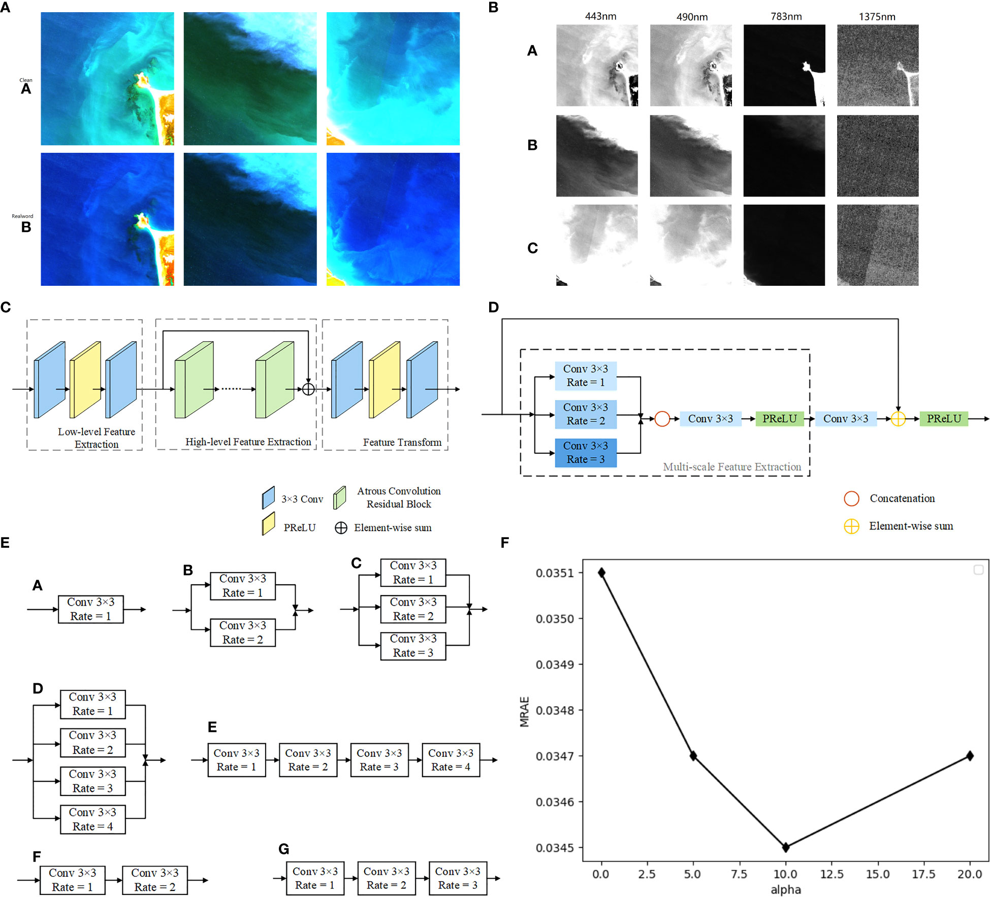
Figure 2 (A) A comparison of the two datasets used in this study ((a) ‘Clean’ and (b) ‘Realworld’) at three locations ((8600, 9300), (10000, 4500), (10300, 900) in UTM zone 52S). (B) Single band hyperspectral data for the 443nm, 490nm,783nm,1375nmbands at (a) coordinates (8600, 9300) (b) (10000, 4500and (c) (10300, 900), all in UTM zone 52S. (C) Overall Structure of MACRN. (D) Structure of the Multi-scale ACRB. (E) Seven kinds of ACRB, (a) C1, (b) C1C2, (c) C1C2C3, (d) C1C2C3C4, (e) C1C2C3C4_S, (f) C1C2_S, (g) C1C2C3_S. (F) Effect of different α values on model reconstruction error.

During MACRN model training, the size of hyperspectral data and RGB image sample pair is 64 × 64 pixels. Overlap area size is 32 pixels when clipping. We performed data enhancement operations such as rotation and mirroring them. The enhancement processing is to rotate within the range of 0° - 180°, the rotation angle is 45°, and make a horizontal flip at each angle at the same time. After enhancement, 1 group 482 × 512 sample pairs generated 3120 groups 64 × 64 sample pairs.

2.2. Problem description

Electromagnetic waves within a certain wavelength range irradiate object surfaces. Because different objects have varying reflectivity to electromagnetic waves of different wavelengths, imaging devices capture the reflection spectra of those surfaces and render images through the conversion of the imaging device. We can express the formation process of the image with Eq. (2.1).

$\begin{array}{ll}{I}_k={\displaystyle {\int }_{\Omega }}E\left(\lambda \right)S{\left(\lambda \right)\text{Φ}}_k\left(\lambda \right)d\lambda & \text{(2.1)}\end{array}$

Where, I_k is the radiant energy recorded by the image sensor k, E(λ) is the spectral energy distribution of the illumination source, S(λ) is the spectral reflectance of the object surface, Φ_k(λ) is the spectral response function of sensor k at the incident wavelength, λ is the wavelength. If the value of λ is an electromagnetic wavelength in the visible light range of 400nm to 700nm, then k corresponds to the image sensors in the R, G and B bands, and we get an RGB image.

The spectral radiation value R(λ) of the target can be obtained by multiplying E(λ) and S(λ); Thus, Eq. (2.1) can be transformed into Eq. (2.2).

$\begin{array}{ll}{I}_k={\displaystyle {\int }_{\Omega }}R{\left(\lambda \right)\text{Φ}}_k\left(\lambda \right)d\lambda & \text{(2.2)}\end{array}$

Discretizing Eq. (2.2) yields:

$\begin{array}{ll}{I}_k={\displaystyle {\sum }_{n}R{\left({\lambda }_n\right)\text{Φ}}_k\left({\lambda }_n\right)}& \text{(2.3)}\end{array}$

Where, λ_n represents the sampled bands. In our study, n has a value of 12 and corresponds to the wavelength range of 443nm to 2190nm.

Therefore, when I_k is known, find R(λ_n). It is a highly uncertain problem to reconstruct the hyperspectral radiation values of 12 bands from RGB images.

We can see that there are huge challenges in how to reconstruct high-precision hyperspectral images from RGB images. Particularly tricky are the problems of insufficient utilization of spatial features of the RGB images, and the unknown spectral response function of the sample data.

We propose a multi-scale atrous convolution residual network (MACRN) model as a solution for obtaining more features of different granularity without introducing too many parameters, with the aim of reconstructing hyperspectral images with greater accuracy.

2.3. Deep learning network

Multiscale network can extract features at different scales, but it also has a high computing cost, and its requirements for computing devices continue to improve. In order to solve this problem, we replace the ordinary convolution kernel with the atrous convolution, which balances the computational cost while extracting multi-scale features.

The overall structure of our multi-scale atrous convolution residual network (MACRN) is shown in Figure 2C. MACRN includes three main parts: low-level feature extraction, high-level feature extraction, and feature transformation.

2.3.1. Low-level feature extraction

The module is composed of a 3 × 3 convolution layer, a PReLU activation function and a 3 x 3 convolution layer. We use it to extract low-level features from the input RGB images, and its expression is shown in Eq. (2.4).

$\begin{array}{ll}y=W_{2}PReLU\left(W_{1}x\right)& \text{(2.4)}\end{array}$

where x is the input, y is the output of the low-level feature extraction, W₁,W₂ is the weight matrix of the two convolution layers in the module, and PReLU is the PReLU activation function.

2.3.2. High-level feature extraction

The module is composed of multiple cascading atrous convolution residual blocks (ACRB). The network is formed through the stacking of multiple modules to extract the high-level features of the input RGB image. The specific structure of the ACRB will be described in detail in Section 2.3. The output of the low-level feature extraction is connected by the global residual and added element by element to the output of the cascaded ACRB to form the final high-level feature set, which can prevent the phenomenon of gradient dispersion and gradient explosion in the deep network architecture. This process is expressed in Eq. (2.5).

$\begin{array}{ll}z=y+f_{ACRB}^N\left(\dots \left(f_{ACRB}^1\left(y\right)\right)\right)& \text{(2.5)}\end{array}$

where, z is the output of the depth feature extraction module, f_ACRB(·) is the atrous convolution residual block, and N is the number of atrous convolution residual blocks.

2.3.3. Feature transformation

The composition of the feature transformation module is the same as that of low-level feature extraction, which is also composed of a 3 x 3 convolution layer, PReLU activation function and a 3 x 3 convolution layer. This module realizes feature transformation and channel integration. The final reconstructed hyperspectral image is formed, and its expression is shown in Eq. (2.6).

$\begin{array}{ll}output=W_{4}PReLU\left(W_{3}z\right)& \text{(2.6)}\end{array}$

where, output is the final output of the whole network, i.e., the hyperspectral image reconstruction result. W₃,W₄ represents two convolution layers respectively, and PReLU represents the PReLU activation function.

2.4. Multi-scale atrous convolution residual block

Currently, most methods for hyperspectral image reconstruction using image blocks have a significant dependence on spatial features ^[33]. When the spatial arrangement of the original image is broken, the reconstruction error often increases greatly, which shows that spatial features play a very important role in the process of hyperspectral image reconstruction. Therefore, the hyperspectral reconstruction error can be further reduced by improving the utilization of spatial features in RGB images.

An important parameter in convolution layers is the size of the convolution kernel, also known as the receptive field, which determines the size of the local area that can be sampled during each iteration. A too small convolution kernel can only extract small local features, while a too large convolution kernel can greatly increase the amount of required computation. Therefore, in order to better extract the spatial features of the image without increasing the computational cost of the network, we use the multi-scale ACRB, which has multiple atrous convolution layers with different atrous rates to control the receptive field. The module can extract the multi-scale spatial features of the image, and then splice the feature maps at different scales to form a multi-scale feature layer. Its structure is shown in Figure 2D.

First, the input characteristic map passes through three 3 x 3 convolution layers with different atrous rates (e.g. the atrous rates for the layers are set to 1, 2 and 3 respectively) to obtain the characteristic f₁, f₂, f₃ at different scales. Then, f₁, f₂, f₃ is spliced together in the channel dimension and integrated through a 3 x 3 convolution layer. Then, the fused multi-scale features are obtained by feature transformation through a PReLU activation function and a 3 x 3 convolution layer. The expression is shown in Eq. (2.7)

$\begin{array}{ll}u=W_6\left(PReLU\left(W_5\left(concat\left[f_1,f_2,f_3\right]\right)\right)\right)& \text{(2.7)}\end{array}$

where, u is the output of the multi-scale feature extraction module in the atrous convolution residual block, W₅,W₆ represents two convolution layers, PReLU represents the PReLU activation function, and concat [,·], represents the channel dimension splicing operation.

To prevent gradient dispersion and gradient explosion, we used a jump connection in the atrous convolution residual block to add the module input and the extracted multi-scale features element by element. The model uses the network fitting residual instead of directly learning the identity mapping function, and its expression is shown in Eq. (2.8).

$\begin{array}{ll}{v}^{\left(n\right)}=PReLU\left(u+v^{\left(n-1\right)}\right)& \text{(2.8)}\end{array}$

where, v⁽ⁿ⁾ is the output of the nth ACRB.

To choose the appropriate multiscale module construction strategy and verify the effectiveness of the results, we designed seven ACRBs with different structures for experiments. We named them C1, C1C2, C1C2C3, C1C2C3C4, C1C2C3_S, C1C2_S, C1C2C3C4_S (Figure 2E).

Through experimental analysis, C1C2C3 proved to be the most effective in our experimental analysis and was used as the basic structure for the multi-scale feature extraction module.

2.5. Loss function

We divided RGB image samples into two sets according to their spectral response functions. The first set was made up of RGB image samples generated using the CIE color function as the spectral response function. We called these images ‘Clean’ data because no noise was added. The second type of data set is called Realworld data, which uses other camera sensitivity functions as spectral response functions and adds noise. The noise type is Gaussian noise, SNR is 30-40dB.

2.5.1. Realworld data

Since the spectral response function in the Realworld data is unknown, the loss function only needs to consider the difference between the reconstructed hyperspectral image and the real hyperspectral image.

RMSE is generally used as the loss function when calculating the error between the predicted image and the real image in the image processing task, given that the image brightness levels of different bands of hyperspectral images are usually quite varied. In the process of calculating the root mean square error, the weight difference between the high brightness region and the low brightness region of the image may be too large. To avoid this situation and balance the deviation between different bands, we use Eq. (2.9) as the loss function of our hyperspectral image reconstruction algorithm:

$\begin{array}{ll}{l}_H=\frac{1}{N}{\displaystyle \sum _{i=1}^n\left(\left|I_R^{(i)}-I_G^{(i)}\right|/I_G^{(i)}\right)}& \text{(2.9)}\end{array}$

where, N represents the total number of pixels, I_R represents the reconstructed spectral radiation value, and I_G represents the spectral radiation value of the actual hyperspectral image.

2.5.2. Clean data

Since the spectral response function Ф for the Clean data is the CIE color function, the loss function needs to take into account the difference between the reconstructed hyperspectral image and the real hyperspectral image, as well as the difference between the RGB images generated by mapping the two types of images to RGB space.

If the spectral response function Ф is known and the RGB image does not contain noise, we can use the function Ф as a priori information to project the reconstructed hyperspectral image into RGB space according to the function Ф. We use Eq. (2.10) to calculate the average absolute error between it and the input RGB image as the loss function.

$\begin{array}{ll}{l}_R=\frac{1}{N}{\displaystyle \sum _{i=1}^n\left(\left|I_R^{(i)}-I_G^{(i)}\right|\right)}& \text{(2.10)}\end{array}$

where, $I_R^{(i)}$ represents the RGB projection of the reconstructed hyperspectral data by matrix multiplication with Ф and $I_G^{(i)}$ represents the RGB projection of real hyperspectral data by matrix multiplication with Ф.

2.5.3. Overall loss function

The overall loss function of our hyperspectral reconstruction model includes l_H and l_R, and its expression is shown in Eq. (2.11)

$\begin{array}{ll}l=l_H+\alpha l_R& \text{(2.11)}\end{array}$

where α is a variable parameter.

We analyzed the influence of different values of α in the loss function Eq. (2.11) of MACRN on the final reconstruction results. Set the value of α to 0, 1, 5, 10 and 20 for experiments, and the results are shown in Figure 2F. It can be seen from the figure that when α is 10, the reconstruction error is the minimum. Therefore, we set the value of α to 10.

3. Results

3.1. Model parameters

Both the low-level feature extraction module and the feature conversion module of MACRN had 256 convolution cores in each convolution layer, while the atrous convolution residual block had 128 in each convolution layer. The images output by the four atrous convolution layers were spliced together to obtain the channel number of the total characteristic image with 512 channels. Then, the number of channels was condensed down to 256 through a convolution layer with 256 convolution cores and a total of six stacked ACRBs.

The batch size for the model training was 16. An Adam optimizer was used for training, with a first-order attenuation index of β₁ = 0.9, a second-order attenuation index of β₂ = 0.9, and a fuzzy factor of ε = 10^-8. The learning rate was initialized to 0.0001, and the polynomial function attenuation strategy was used to gradually reduce the learning rate during the training process.

3.2. Quantitative analysis of ACRB

To determine how the number of atrous convolution residual blocks (ACRB) affects the hyperspectral image reconstruction model, we constructed five hyperspectral reconstruction networks with different depths with the number of ACRB ranging from four to eight, which were chosen considering the poor feature extraction ability of the low-level network. The test results are shown in Figure 3A.

FIGURE 3

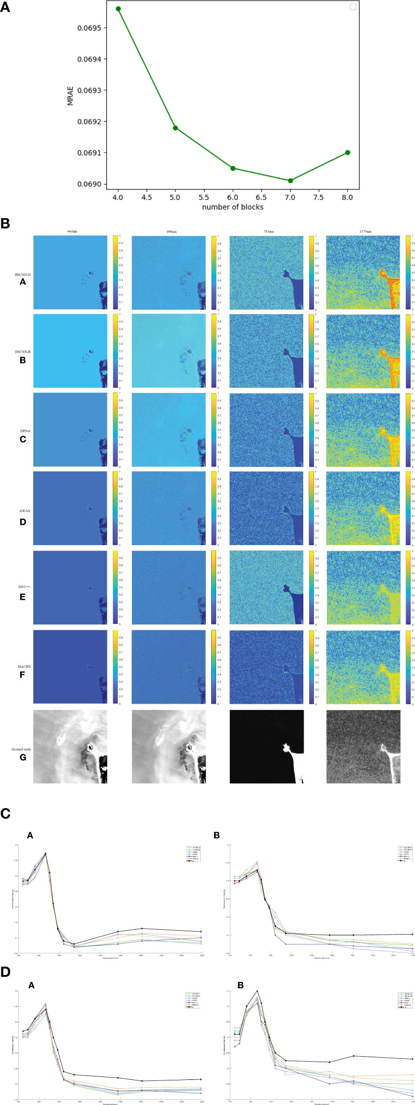
Figure 3 (A) Reconstruction error of different ARCB numbers. (B) Error image (heat map) of hyperspectral image reconstructions and real hyperspectral images of (from left to right) the 443 nm, 490 nm, 783 nm and 1375 nm bands by the (a) HSCNN-D, (b) HSCNN-R, (c) HRNet, (d) AWAN, (e) MACRN models run on images from the Clean dataset, compared to (f) the true hyperspectral data of the same locations. (C) Spectral response curve from the HSCNN-D, HSCNN-R, HRNet, AWAN, MACRN models run on Clean data and true observed data from Sentinel-2 (gt for ground truth) for two points from the images shown in Figure 3.2, (a) coordinates (312, 315) and (b) (764, 494). (D) Spectral response curves from HSCNN-D, HSCNN-R, HRNet, AWAN, MACRN run on Realworld data, and observed data (gt) from two points from Figure 3.2, (a) coordinates (312,315) and (b) (764,494).

In Figure 3A, MRAE (Mean Relative Absolute Error) is a commonly used index to evaluate spectral reconstruction effect, and RMSE (Root Mean Square Error) is used as an auxiliary evaluation standard.

The reconstructed MRAE error reached the minimum at seven ACRB (Fig. 3.1). However, there was very little difference between six and seven ACRBs, so in order to minimize the number of parameters and reduce the complexity of the model, the number of stacks for the ACRB is set to 6.

3.3. Clean data reconstruction

In order to evaluate how the MACRN model against to other reconstruction algorithms, we compared it to HSCNN-R (Shi et al., 2018), HSCNN-D (Shi et al., 2018), HRNet (Zhao et al., 2020), AWAN (Li et al., 2020), MST++ (Cai et al., 2022). To ensure the fairness of the experiment, all models were run under the same experimental conditions, using the same training and test sets.

The MACRN model obtained the lowest error value on the Clean data (Table 1). The HSCNN-R model had the shortest running time, but a large error rate. The AWAN model had the second fastest running time, but MACRN was almost as quick. In conclusion, the MACRN performs well in spectral reconstruction of Clean data.

TABLE 1

Table 1 Comparison of reconstruction results of various models run on the Clean dataset.

Figure 3B shows the a heat map (error image) of the hyperspectral images reconstructed from the Clean data for the six models and the real hyperspectral image (Ground truth) in the bands of 443 nm, 490 nm, 783nm and 1375nm.

The error of the reconstructed hyperspectral image in the bands of 443 nm, 490 nm and 783nm was small, while the error in the 1375 nm band was large (Figure 3B). Overall, MACRN produced a high quality reconstruction.

Figure 3C shows the spectral response curves drawn at two spatial positions from the hyperspectral images reconstructed by Clean data of five models. The reconstructed spectral curves of MACRN closely matched the real spectral curves, demonstrating its accuracy in spectral reconstruction relative to the other four models (Figure 3C).

3.4. Realworld data reconstruction

From the Realworld data, MACRN exhibited the smallest errors of the six models (Table 2). HSCNN-R again had the shortest running time, but its reconstruction error was large. The running time of MACRN was close to that of HRNet.

TABLE 2

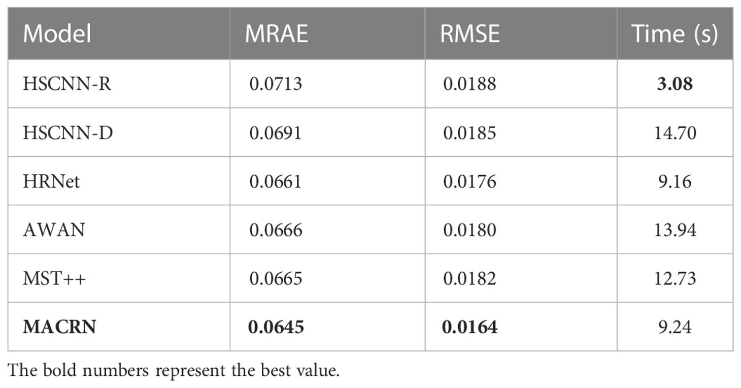
Table 2 Comparison of reconstruction results of various models run with the Realworld dataset.

Figure 3D shows the spectral response curves drawn at two spatial positions from the hyperspectral images reconstructed from Realworld data of five models.

All models had higher error rates when run with Realworld data than with Clean data (Fig. 3.4). Compared with other methods, MACRN had the closest fit to the true values (Figure 3D).

The MACRN realizes hyperspectral spectral reconstruction in 443nm - 2190nm band, with less computation and high reconstruction accuracy. On the Realworld dataset, the reconstruction error MARE index is less than 0.0645, the reconstruction error RMSE index is less than 0.0164, and the reconstruction time is less than 9.24S. On the Clean dataset, the reconstruction error MARE index is less than 0.0328, the reconstruction error RMSE index is less than 0.0114, and the reconstruction time is less than 8.58S.

To sum up, for both Clean data and Realworld data sets, the performance of MACRN hyperspectral reconstruction algorithm was relatively stable, and offered good hyperspectral reconstruction relative to other models.

4. Discussion

Tables 1 and 2 show that the calculation cost of MACRN reconstruction algorithm is small. Figures 3C, D show that the error between the reconstructed spectral curve of MACRN and the actual spectral curve is small. In the visible light band, the MACRN reconstruction error has no difference with MST++ (Cai et al., 2022) and AWAN (Li et al., 2020), and is close to the true value. However, in the near infrared band, the MACRN reconstruction accuracy is significantly better than other spectral reconstruction algorithms. Although MST++ (Cai et al., 2022) based on spatial sparsity and spectral self similarity won the first in the RGB spectral reconstruction challenge in 2022. However, MST++ ignored some spatial details and did not consider the near-infrared and mid infrared band features. Therefore, the hyperspectral reconstruction result of MST++ is obviously inferior to those of MACRN in the near infrared and mid infrared bands. This fully shows that ACRB of MACRN captures more spatial details, and the loss function of MACRN is more consistent with the characteristics of the near infrared and mid infrared spectrum.

In the detection application of marine water quality (such as chlorophyll-a, dissolved organic matter, solid suspended solids, etc.), it is easier to find target differences in the near-infrared band, and the reconstruction algorithm that can accurately reconstruct the target’s near-infrared band spectrum has a greater application prospect. For example, in marine oil pollution detection (Guga, 2020), because hyperspectral images can obtain a large amount of nearly continuous narrowband spectral information in the visible, near infrared, mid infrared and thermal infrared bands. The hyperspectral images can not only effectively distinguish oil film and water, but also infer the type and time of oil leakage from the different spectral absorption characteristics of offshore oil film. We use the MACRN algorithm to construct hyperspectral images, which can easily and quickly detect and identify objects based on the spectral characteristics. Therefore, the MACRN hyperspectral reconstruction algorithm has the characteristics of low reconstruction cost and high reconstruction accuracy, and its advantages in marine spectral reconstruction are more obvious.

5. Conclusion

The reconstruction of high-precision hyperspectral images from RGB images is important for expanding the use of hyperspectral analysis in the marine sciences. Currently, most algorithms of reconstructing hyperspectral images from RGB images use convolution neural networks, which is problematic because the receptive field of the convolution kernel is at a small, fixed scale, and thus can only learn the features at a single scale, offers low utilization of information from a global context, and lacks global vision.

We designed a hyperspectral image reconstruction algorithm based on a multi-scale atrous convolution residual network (MACRN), which can better solve one of the problems. The algorithm extracts multi-scale features under different receptive fields, makes full use of the rich colors of RGB images and the spatial structure associated with the colors, and adds richer contextual information, ensuring the integrity of local details. Our hyperspectral reconstruction experiment using Sentinel-2 satellite data from the northern coast of Australia shows that the algorithm can effectively reduce hyperspectral reconstruction errors and deliver hyperspectral image reconstruction of high-precision RGB images with low computational costs.

Data availability statement

The original contributions presented in the study are included in the article/supplementary material. Further inquiries can be directed to the corresponding author.

Author contributions

All authors listed have made a substantial, direct, and intellectual contribution to the work and approved it for publication.

Acknowledgments

This research is supported by Sichuan Science and Technology Program (2022NSFSC0020), Chengdu Science and Technology Program (2022-YF09-00019-SN), and the Chengdu Research Base of Giant Panda Breeding (NO. 2020CPB-C09, NO. 2021CPB-B06). We would like to thank Dr. Annalise Elliot at the University of Kansas for her assistance with English language and grammatical editing of the manuscript.

Conflict of interest

The authors declare that the research was conducted in the absence of any commercial or financial relationships that could be construed as a potential conflict of interest.

Publisher’s note

All claims expressed in this article are solely those of the authors and do not necessarily represent those of their affiliated organizations, or those of the publisher, the editors and the reviewers. Any product that may be evaluated in this article, or claim that may be made by its manufacturer, is not guaranteed or endorsed by the publisher.

References

Aeschbacher J., Wu J., Timofte R. (2017). “In defense of shallow learned spectral reconstruction from rgb images,” in International Conference on Computer Vision Workshops. (Venice, Italy: ICCVW) 471–479.

Google Scholar

Agahian F., Arnirshahi S. A., Amirshahi S. H. (2008). Reconstruction of reflectance spectra using weighted principal component analysis. Color Res. Appl. 33 (5), 360–371. doi: 10.1002/col.20431

CrossRef Full Text | Google Scholar

Alvarezgila A., Weijer J., Garrote E. (2017). “Adversarial networks for spatial context-aware spectral image reconstruction from rgb,” in 2017 IEEE International Conference on Computer Vision Workshops (ICCVW). (Venice, Italy: ICCVW). 480–490.

Google Scholar

Antonio R. (2015). “Single image spectral reconstruction for multimedia applications,” in Proceedings of the 23rd ACM international conference on Multimedia. (Brisbane: ASSOC Computing Machinery, Australia) 251–260.

Google Scholar

Arad B., Benshahar O. (2016). “Sparse recovery of hyperspectral signal from natural RGB images,” in European Conference on Computer Vision. (Amsterdam, Netherlands: Springer-Verlag Berlin) 19–34.

Google Scholar

Beletkaia E., Pozo J. (2020). More than meets the eye: Applications enabled by the non-stop development of hyperspectral imaging technology. PhotonicsViews 17 (1), 24–26. doi: 10.1002/phvs.202070107

CrossRef Full Text | Google Scholar

Cai Y., Lin J., Lin Z. (2022). MST++: Multi-stage spectral-wise transformer for efficient spectral reconstruction. CVPR. doi: 10.1109/CVPRW56347.2022.00090

CrossRef Full Text | Google Scholar

Descour M., Dereniak E. (1995). Computed-tomography imaging spectrometer: experimental calibration and reconstruction results. Appl. optics 34 (22), 4817–4826. doi: 10.1364/AO.34.004817

CrossRef Full Text | Google Scholar

Galliani S., Lanaras C., Marmanis D., Baltsavias E., Schindler K. (2017). Learned spectral super-resolution[EB/OL]. ArXiv 03–28. doi: 10.48550/arXiv.1703.09470

CrossRef Full Text | Google Scholar

Geelen B., Tack N., Lambrechts A. (2014). Acompact snapshot multispectral imager with a monolithically integrated per-pixel filter mosaic. Advanced Fabrication Technol. Micro/Nano Optics&Photonics VII Int. Soc. Optics Photonics, (Osaka, Japan) 661–674. doi: 10.1117/12.2037607

CrossRef Full Text | Google Scholar

Goel M., Whitmire E., Mariakakis A, Saponas T. S., Joshi N., Morris D., et al. (2015). “Hypercam: hyperspectral imaging for ubiquitous computing applications,” in Proceedings of the 2015 ACM International Joint Conference on Pervasive and Ubiquitous Computing (Osaka, Japan) 145–156.

Google Scholar

Guga S. (2020). Extraction of marine oil spill information by hyperspectral mixed pixel decomposition. Inner Mongolia Sci. Technol. and Economy 02, 84–89.

Google Scholar

Huang T., Dong W., Yuan X. (2021)Deep Gaussian scale mixture prior for spectral compressive imaging. 2021 IEEE/CVF Conference on Computer Vision and Pattern Recognition (CVPR).

Google Scholar

Jia Y., Zheng Y. Q., Gu L., Subpa-Asa A., Lam A., Sato Y., Sato I., et al. (2017). “From rgb to spectrum for natural scenes via manifold-based mapping,” in Proceedings of the IEEE International Conference on Computer Vision. (Venice, Italy: ICCV) 4705–4713.

Google Scholar

Kaya B., Can Y., Timofte R. (2019). “Towards spectral estimation from a single rgb image in the wild,” in 2019 IEEE/CVF International Conference on Computer Vision Workshop. (Seoul, South Korea: ICCVW) 3546–3555.

Google Scholar

Li J. J., Wu C. X., Song R, Li Y. S., Liu F. (2020). “Adaptive weighted attention network with camera spectral sensitivity prior for spectral reconstruction from RGB images,” in 2020 IEEE/CVF Conference on Computer Vision and Pattern Recognition Workshops (CVPRW). (ELECTR Network) 1894–1903.

Google Scholar

Nguyen R., Prasad D., Brown M. (2014). “Training-based spectral reconstruction from a single RGB image,” in European Conference on Computer Vision. (Zurich, Switzerland) 186–201.

Google Scholar

Oh S. W., Brown M. S., Pollefeys M., Kim S. J. (2016). “Do it yourself hyperspectral imaging with everyday digital cameras,” in Computer Vision and Pattern Recognition, (Las Vegas Seattle, WA). 1063–1069.

Google Scholar

Pengfei L., Huaici Z., Peixuan Li (2020). Hyperspectral images reconstruction using adversarial networks from single RGB image. Infrared Laser Eng. 49 (S1), 143–150. doi: 10.3788/IRLA20200093

CrossRef Full Text | Google Scholar

Peterson K. T., Sagan V., Sloan J. J. (2020) Deep learning-based water quality estimation and anomaly detection using landsat-8/Sentinel-2 virtual constellation and cloud computing. GISCIENCE Remote Sens. 202, 510–525. doi: 10.1080/15481603.2020.1738061

CrossRef Full Text | Google Scholar

Qizhong Z., Endi Z., Yejian W., Farong G. (2021). Recognition of ocean floor manganese nodules by deep kernel fuzzy c-means clustering of hyperspectral images. J. Image Graphics 26 (08).

Google Scholar

Shi Z., Chen C., Xiong Z. W., Liu D., Wu F. (2018). “Hscnn+: Advanced cnn-based hyperspectral recovery from rgb images,” in 2018 IEEE/CVF Conference on Computer Vision and Pattern Recognition Workshops. (Salt Lake City, UT: CVPRW) 1052–1058.

Google Scholar

Shoeiby M., Robles-Kelly A., Timofte R., Zhou R. F., Lahoud F., Susstrunk S., et al. (2018a). “Pirm2018 challenge on spectral image super-resolution: Methods and results,” in The European Conference on Computer Vision (ECCV) Workshops. (Munich, Germany) 56–371.

Google Scholar

Shoeiby M., Robles-Kelly A., Wei R., Timofte R. (2018b). “Pirm2018 challenge on spectral image super-resolution: Dataset and study,” in The European Conference on Computer Vision (ECCV) Workshops. (Munich, Germany) 276–287.

Google Scholar

Veronez M. R., Kupssinsku L. S., Guimaraes T. T. (2018). Proposal of a method to determine the correlation between total suspended solids and dissolved organic matter in water bodies from spectral imaging and artificial neural networks. SENSORS. doi: 10.3390/s18010159

CrossRef Full Text | Google Scholar

Xiong Z. W., Shi Z., Li H. Q., Wang L. Z., Liu D., Wu F., et al. (2017). “HSCNN: CNN-based hyperspectral image recovery from spectrally undersampled projections,” in 2017 IEEE International Conference on Computer Vision Workshops (ICCVW), Venice, Italy. 518–525.

Google Scholar

Ying H. T., Xia K., Huang X. X. (2021). Evaluation of water quality based on UAV images and the IMP-MPP algorithm. Ecol. Inf. 61, 101239. doi: 10.1016/j.ecoinf.2021.101239

CrossRef Full Text | Google Scholar

Zhao Y., Po L., Yan Q. (2020). “Hierarchical regression network for spectral reconstruction from RGB images,” in IEEE/CVF Conference on Computer Vision and Pattern Recognition Workshops (CVPRW). (ELECTR Network) 1695–1704.

Google Scholar