Offshore wind farms changed the spatial distribution of chlorophyll-a on the sea surface

Introduction

The construction of OWFs plays an important role in reducing carbon emissions (Li et al., 2022), so there has been large-scale construction of OWFs in recent years. However, the development of OWFs has impacts on marine organisms (Andersson, 2011; Tricas and Gill, 2011; Coates et al., 2014; Raoux et al., 2017; Oh et al., 2021; Pollock et al., 2021), marine water quality (Kamermans et al., 2018), birds (Furness et al., 2013) and sediments (De Borger et al., 2021). In particular, OWFs adversely affect the marine ecological environment and the behavior, physiology, growth and survival of marine organisms (Methratta and Dardick, 2019; Mavraki et al., 2020). Previous studies have played a very positive role in promoting the sustainable development of OWFs. That is, changes in local marine dynamics at the turbine base may affect the behavior, distribution and physiological state of marine animals (Methratta and Dardick, 2019), and local climate changes may be caused by fan operation. OWFs ultimately affect the marine environment and marine ecosystem by changing the local climate and marine dynamics (Degraer et al., 2020; van Berkel et al., 2020). However, due to the complexity of dynamic marine monitoring and the diversity of marine environment evaluation indicators, it is difficult to accurately evaluate the impact of wind farms on marine ecosystems and the marine environment. Therefore, a more detailed analysis of the impacts of OWFs on representative factors of the marine environment may play an important role in better understanding the impacts of wind farms on marine ecosystems (Fishman and Graedel, 2019; Pryor et al., 2020).

Chlorophyll-a (Chl-a) is one of the main dye in phytoplankton and an indicator of marine primary productivity and an important parameter for evaluating the degree of marine water quality and organic pollution (Zhang et al., 2019; Wang et al., 2020). The spatial distribution pattern of seawater Chl-a is a reflection of basic marine spatial information and determines the distribution status and production capacity of offshore living resources at different spatial levels (Zhang et al., 2019; Callbeck et al., 2021). Therefore, the evaluation of the impact of OWFs on the spatial distribution pattern of Chl-a would be of significance.

Benassai et al. (2014) used MERIS data when determining the correlation between the OWFs in Europe and the sustainability index and found an increasing trend in the concentration of Chl-a in the vicinity of the OWF in the North Sea (Benassai et al., 2014). Floeter et al. (2017) also found that the concentration of Chl-a near the North Sea OWF increased by combining the measured Chl-a with a MODIS image. Additionally, they proposed that the increase in Chl-a concentration near OWFs was probably the result of the upwelling of lower phytoplankton (Floeter et al., 2017). This prior research is helpful to determine the impact of OWFs on marine ecology. However, the Chl-a of OWFs is greatly affected by tidal currents and waves and verification of these findings, for example with high spatial resolution, through numerous studies and considering global OWF distribution areas, is lacking. Therefore, the present study used Landsat data from 1990 to 2021 to calculate the Chl-a concentration of typical OWFs around the world and applied this to determine the impact of OWFs on the spatial distribution of Chl-a on the sea surface.

Data and methods

Data resources

Landsat 5 and Landsat 8 data: From Landsat 5 and Landsat 8 data from the Google Earth Engine (GEE) platform from 1990 to 2021, remote sensing images with cloud cover of less than 5% were selected. These included 423 Landsat 5 images from 1990 to 2012 and 259 Landsat 8 images from 2013 to 2021.

Offshore wind farms (OWF) locations: A global OWF dataset was developed using geospatial technology and advanced mathematical operations on the GEE platform using earth observation Sentinel 1 SAR time-series imagery. It was verified that the extraction accuracy of this data set exceeded 99% (Zhang et al., 2021).

Study area

OWFs in Europe and China were selected as the research object. These OWFs were divided according to their construction date. The OWFs in Europe were denoted WF1–WF36 and those in China were denoted WF37–WF38. The total number of Offshore wind turbines(OWTs) in the OWFs was 4263, accounting for 85.4% of global OWTs (Díaz and Guedes Soares, 2020). The location of the study area is shown in Figure 1.

FIGURE 1

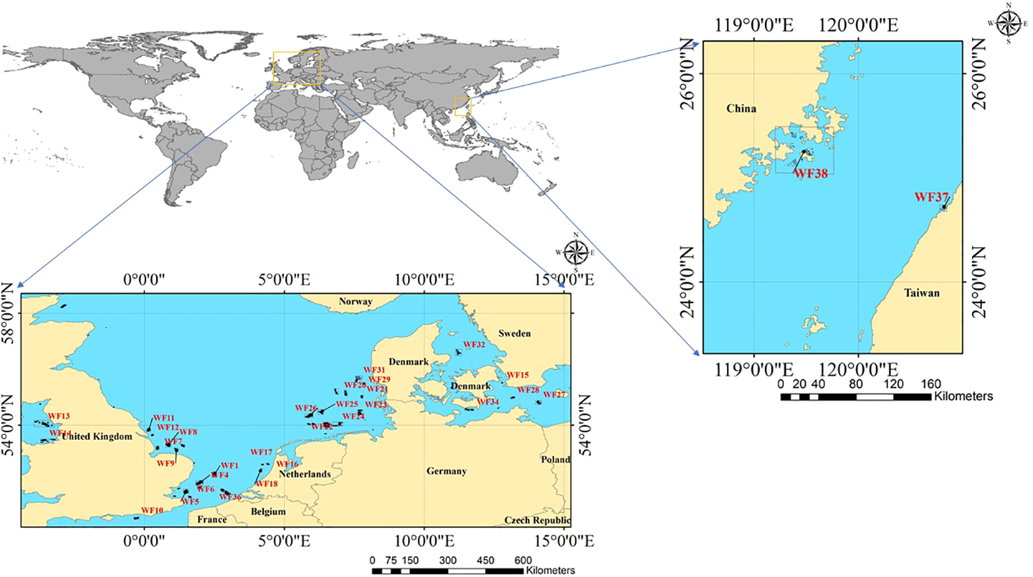
Figure 1 Location map of OWFs.

Methods

Calculation of Chl-a

OC2 algorithm and HU color index (CI) algorithm are used in this paper. When Chl-a > 0.3 mg·m^–3, the O’Reilly band ratio OC2 algorithm was used, as shown in equation (1) (O’Reilly et al., 2000).

$\begin{array}{ll}\begin{array}{l}Ch{l}_{OC2}={10}^y\\ \text{y}={\text{a}}_0+{\text{a}}_{1}x+{\text{a}}_2{x}^2+{\text{a}}_3{x}^3+{\text{a}}_4{x}^4\\ \text{x}={\text{log}}_{10}\left(\frac{{\text{Rrs(λ}}_{blue})}{{\text{Rrs(λ}}_{green})}\right)\end{array}& (1)\end{array}$

The OC2 algorithm is a fourth-order polynomial relationship between a ratio of Rrs and Chl-a. The terms a₀–a₄ are derived from the NASA Ocean Color website (https://oceancolor.gsfc.nasa.gov/atbd/chlor_a/) and were a₀ = 0.1977, a₁ = –1.8117, a₂ = 1.9743, a₃ = –2.5635 and a₄ = –0.7218 in the Landsat sensor.

When 0 mg·m^–3< Chl-a ≤ 0.25 mg·m^–3, the HU color index (CI) algorithm was used, as shown in equation (2) (Hu et al., 2012).

$\begin{array}{ll}Ch{l}_{\text{CI}}={10}^{-0.4909+191.659*CI}& (2)\end{array}$

Here, Chl_CI is the concentration of Chl-a calculated by HU color index (CI) algorithm, as shown in equation (3). (Hu, 2011)

$\begin{array}{ll}\text{CI}={\text{Rrs(λ}}_{green})-[{\text{Rrs(λ}}_{blue})+({\text{λ}}_{green}-{\text{λ}}_{blue})/({\text{λ}}_{red}-{\text{λ}}_{blue})*\left({\text{Rrs(λ}}_{red})-{\text{Rrs(λ}}_{blue})\right)]& (3)\end{array}$

The CI value in equation (2) is derived from equation (3). (Hu, 2011) Rrs is the surface reflectance, where λ_blue, λ_green and λ_red are the instrument-specific wavelengths closest to 443, 555 and 670 nm, respectively; these correspond to the blue, green and red wavelength bands λ_blue, λ_green and λ_red in the Landsat satellite, respectively.

When 0.25 mg·m^–3< Chl-a ≤ 0.3mg·m^–3, a hybrid algorithm of the two algorithms was used, as shown in equation (4).

$\begin{array}{ll}Chl–a=\text{α}\times Ch{l}_{OC2}+\beta \times Ch{l}_{CI}& (4)\end{array}$

Here, α = (Chl_CI – 0.25)/(0.05) and β = (0.3 – Chl_CI)/(0.05) (Hu et al., 2012). Finally, equation (5) for calculating the Chl-a of the sea surface was obtained.

$\begin{array}{ll}\begin{array}{l}Chl–a=Ch{l}_{\text{CI}}[for0<{\text{Chl}}_{CI}\le 0.25mg{m}^{-3}]\\ Ch{l}_{OC2}\text{ [}forCh{l}_{CI}>0.3mg{m}^{-3}]\\ \text{α}\times Ch{l}_{OC2}+\beta \times Ch{l}_{\text{CI}}\text{ [}for0.25<Ch{l}_{CI}\le 0.3mg{m}^{-3}]\end{array}& (5)\end{array}$

This refinement was restricted to relatively clear water and the general impact was to reduce artifacts and biases in clear-water chlorophyll retrievals due to residual glint, stray light, atmospheric correction errors, and white or spectrally-linear bias errors in Rrs. In this algorithm, the value range was first determined by the Chl-a concentration calculated by CI algorithm, and then the algorithm was selected to calculate according to different value ranges.

The OC2 and CI algorithms not only have high accuracy, but also can smooth and smooth the transition in different Chl-a ranges(https://oceancolor.gsfc.nasa.gov/atbd/chlor_a/). After that, the algorithm was adopted by multiple studies, and the CI algorithm performed better in low-concentration Chl-a (< 0.25 mg•m^-3). Brewin et al. evaluated the inversion precision of Chl-a in the Red Sea using this algorithm, and found that the precision and accuracy of the algorithm in the Red Sea were comparable to those in the global ocean (Brewin et al., 2013). Seegers et al. compared the global oceanic Chl-a data acquired by different algorithms and adopted the in-situ measurement data set of Chl-a for verification, and found that the error between the results of HU algorithm and OC algorithm was the lowest (Seegers et al., 2018). In addition, many studies show that the Chl-a algorithm based on CI in this paper further reduces the instrument noise and the error caused by atmospheric correction (Brewin et al., 2016; Wang and Son, 2016). Therefore, we believe that the Chl-a algorithm used in this paper is reasonable and can obtain accurate results.

Global Moran’s I

The global Moran’s index (I) is a rational number. After variance normalization, its value will be normalized to between –1.0 and 1.0 (Moran, 1950). Values in the [–1,0] interval have a negative spatial correlation and values in the [0,1] interval have a positive spatial correlation. The larger the value, the higher the spatial correlation. Moran’s I is calculated using equation (6).

$\begin{array}{ll}I=\frac{n}{{\displaystyle {\sum }_{i=1}^n{\displaystyle {\sum }_{j=1}^n{w}_{ij}}}}\times \frac{{\displaystyle {\sum }_{i=1}^n{\displaystyle {\sum }_{j=1}^n{w}_{ij}(y_i-\overline{y})(y_j-\overline{y})}}}{{\displaystyle {\sum }_{i=1}^n{(y_i-\overline{y})}^2}}& (6)\end{array}$

Here, n is the total number of regional units. y_i and y_jare random variables that are the attribute values in geographic units i and j; in this study, i and j were the Chl-a concentration values of the geographic unit. y is the average value of the sample attribute values of n spatial units; that is, the average Chl-a concentration in the whole OWF. w_ijis the weight matrix of geographical units adjacent to each other; that is, the spatial weight value (Anselin, 2019).

Local Moran’s I

The local Moran’s I was used to analyses the impact of OWFs on Chl-a concentration in their region. The calculation of the local Moran’s index passed the significance test (p ≤ 0.05) and output the results, which were divided into four types:high-value (HH) clustering, low-value (LL)clustering and abnormal values (HL) where the high value is mainly surrounded by low value, and abnormal value (LH) where the low value is mainly surrounded by high value (Khosravi et al., 2018). In this study, HH and LL patterns represented spatial aggregates of Chl-a with high and low values at the center, respectively. HL mode represents Chl-a outliers with high values mainly surrounded by low values and the LH mode represented Chl-a outliers with low values mainly surrounded by high values.

The local Moran’s I of region i is calculated using equation (7).

$\begin{array}{ll}{I}_i=\frac{(y_i-\overline{y})}{\frac{1}{n}{\displaystyle \sum {(y_i-\overline{y})}^2}}{\displaystyle \sum _{i\ne j}^n{w}_{ij}(y_j-\overline{y})}& (7)\end{array}$

Here, n is the total number of Chl-a pixels in the OWFs’ areas. y_i and y_j are the attribute values of the i^th geographical unit and the j^th geographical unit; that is, the concentration of Chl-a. y is the average value of the sample attribute values of n spatial units; that is, the average Chl-a concentration in the whole OWF area. w_ij is the spatial weight value (Anselin, 1995).

Using the O’Reilly band ratio OC2 algorithm and HU CI algorithm, the Chl-a concentrations of the Landsat 5 and Landsat 8 data from the GEE platform were calculated (https://code.earthengine.google.com/chla). All Landsat data have been atmospheric corrected. These calculated results were exported to the local computer and the global Moran’s I and local Moran’s I were then calculated using ArcGIS10.7.

Results

Spatial autocorrelation of Chl-a in OWFs increased

According to the construction date of the OWFs, the global Moran’s I was divided into pre-construction and post-construction. The mean and standard deviation of the global Moran’s I before and after construction are shown in Figure 2. The average value of the global Moran’s I increased by different degrees after the wind farms are built. The global Moran’s I increased for 97.3% of all OWFs. Compared with before the construction, the global Moran’s I after the construction of the OWFs had a maximum value of 0.665 and a minimum value of 0.003. Therefore, it was concluded that the construction of the OWFs has an impact on the spatial distribution pattern of Chl-a.

FIGURE 2

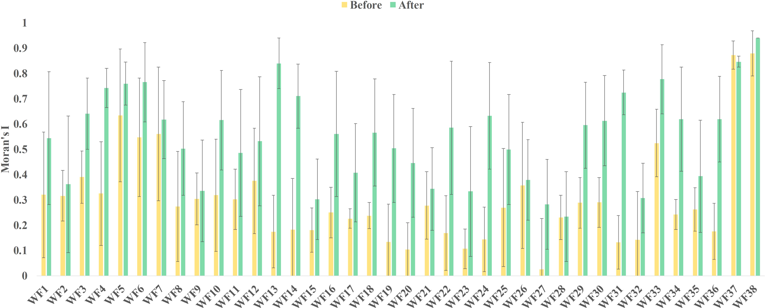
Figure 2 Mean change in global Moran’s I before and after OWF construction.

Aggregation of Chl-a at OWFs

Based on the global Moran’s I, the local Moran’s I results of 38 study areas were compared and analyzed. The number of pixels of high-value clustering (HH) and low-value clustering (LL) in each study area were counted and it was found that the spatial distribution pattern of Chl-a at 73.7% OWFs and the number of HH and LL pixels had increased significantly, as shown in Figure 3. A comparison of the average values of HH and LL before and after OWF construction revealed that the number of HH pixels increased by 90.7% while the number of LL pixels increased by 68.9%. This indicated that HH and LL increased in the spatial distribution pattern of Chl-a concentration and that HH increased more than LL for these OWFs. Therefore, it appeared that the construction of OWFs resulted in significant aggregations of Chl-a.

FIGURE 3

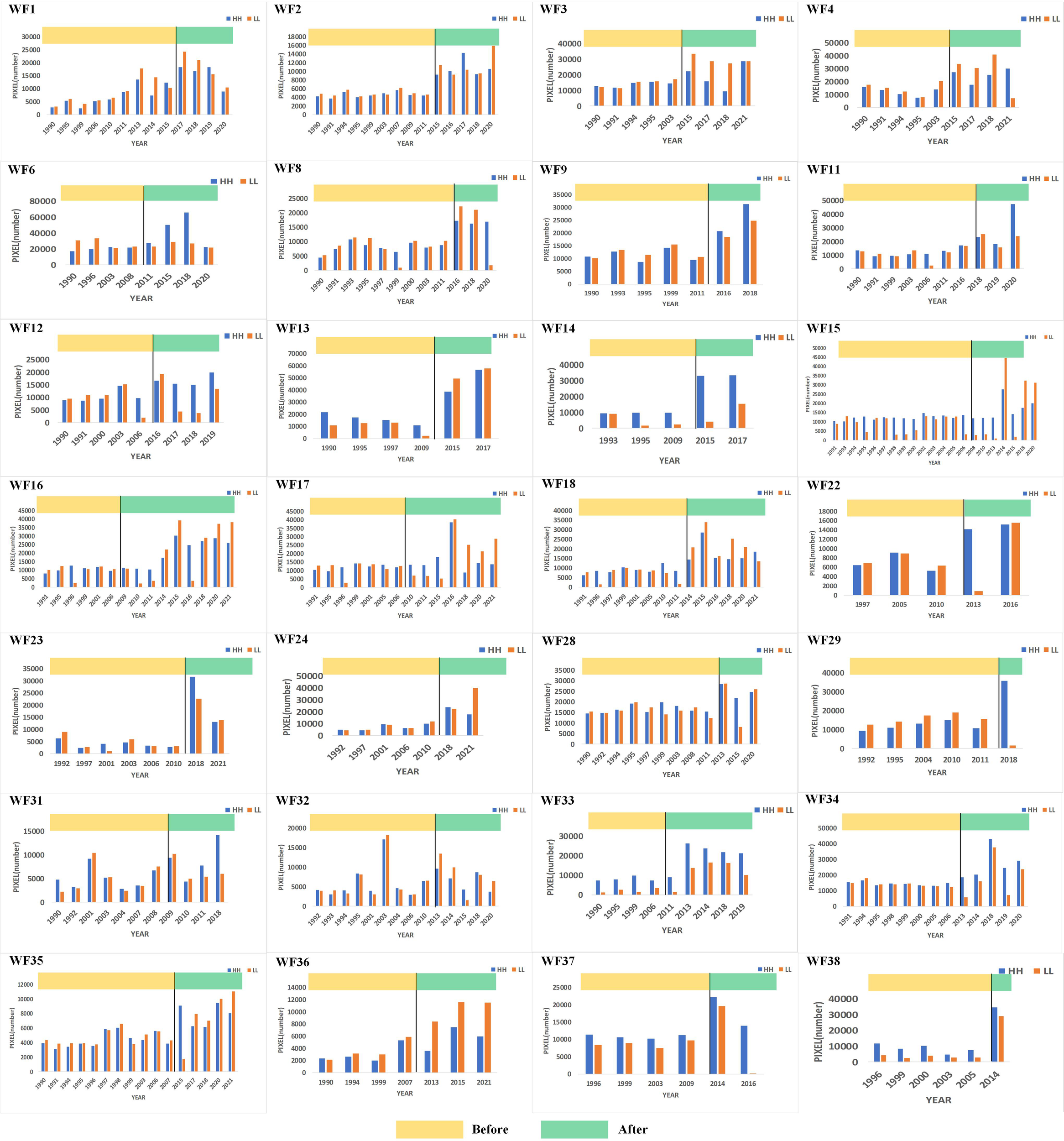
Figure 3 Spatial distribution pattern of Chl-a showing obvious aggregation before and after OWF construction.

To determine the spatial aggregation changes of Chl-a before and after OWF construction, the local Moran’s I aggregation pattern of the above OWFs was also compared, some typical OWFs as shown in Figure 4. The aggregation of Chl-a changed significantly after OWF construction compared with that before OWF construction. The distribution of HH and LL pixels before OWF construction was scattered but, after OWF construction, HH and LL pixels were aggregated. This indicated that high and low concentrations of Chl-a accumulated spatially. Therefore, through the above comparative analysis, it was concluded that the construction of OWFs affected the spatial distribution pattern of Chl-a.

FIGURE 4

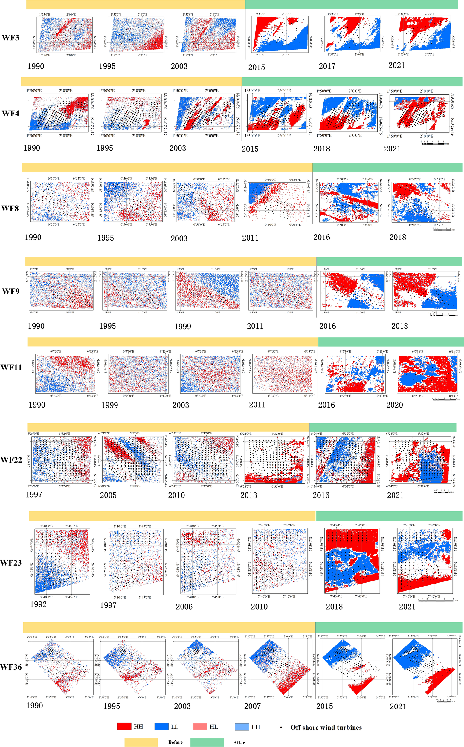
Figure 4 The local Moran’s I aggregation pattern before and after OWF construction.

The local Moran’s I analysis results of the 28 OWFs revealed that there was a higher concentration of Chl-a after OWF construction than before. Not only was there an increase in the number of HH and LL pixels but HH and LL pixels also had more concentrated spatial distribution patterns than before construction. Therefore, it was concluded that OWF construction led to the aggregation of Chl-a.

Areas with no significant aggregation of Chl-a

According to the local Moran’s I results, there were 10 OWFs where Chl-a did not show significant aggregation. Therefore, the same method as used above was used to compare the changes in the local Moran’s I within these OWFs. The results are shown in Figure 5.

FIGURE 5

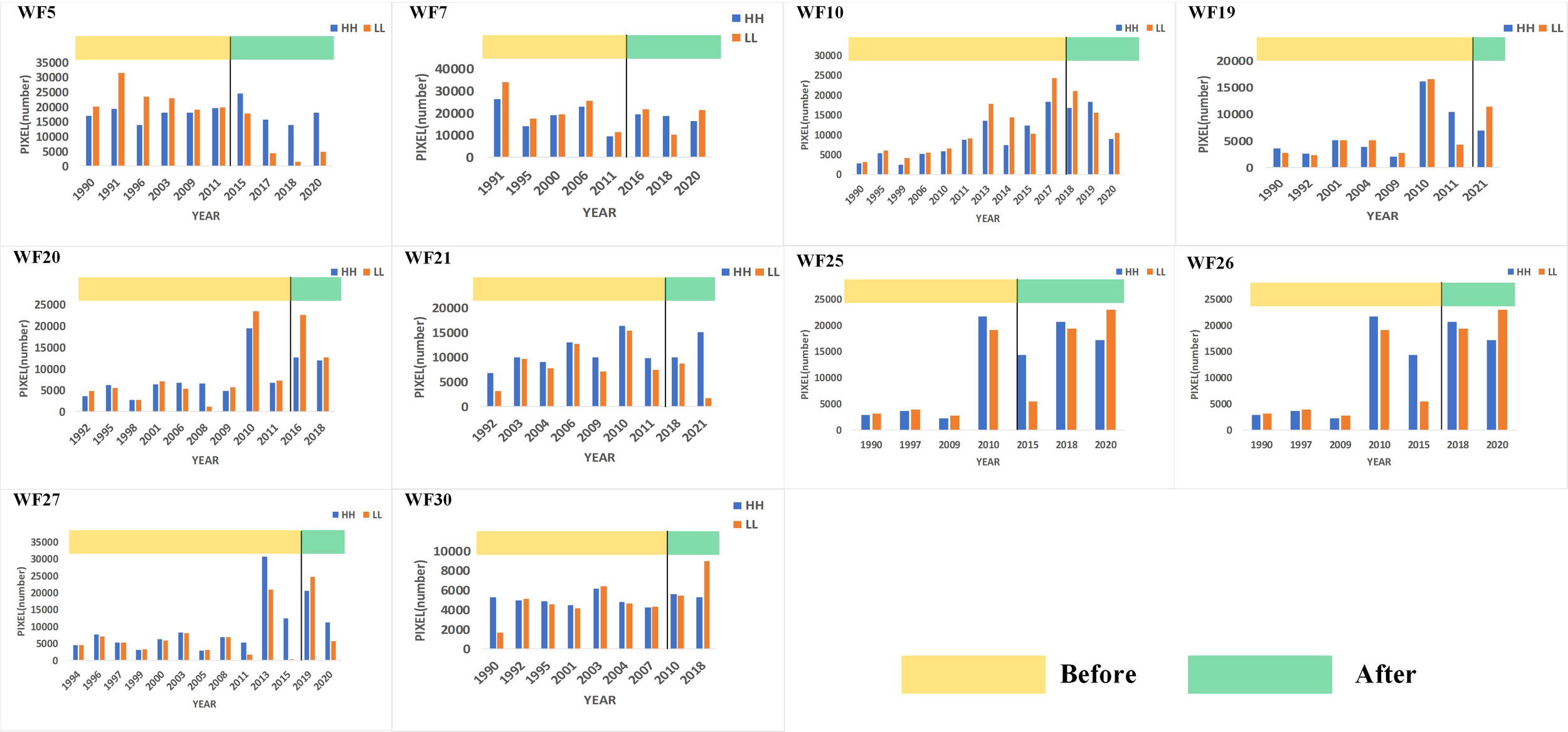
Figure 5 Spatial distribution pattern of Chl-a showing no obvious changes after OWF construction.

The changes in the number of HH and LL pixels had no unified trend and no significant increase in the number of HH and LL pixels was found (Figure 5). There was no obvious change in the spatial distribution pattern of Chl-a before and after OWF construction and even a decrease in the number of HH and LL pixels was observed after the construction of some OWFs, such as WF5. To further explore this phenomenon, spatial HH and LL changes based on the local Moran’s I were compared, some typical OWFs as shown in Figure 6.

FIGURE 6

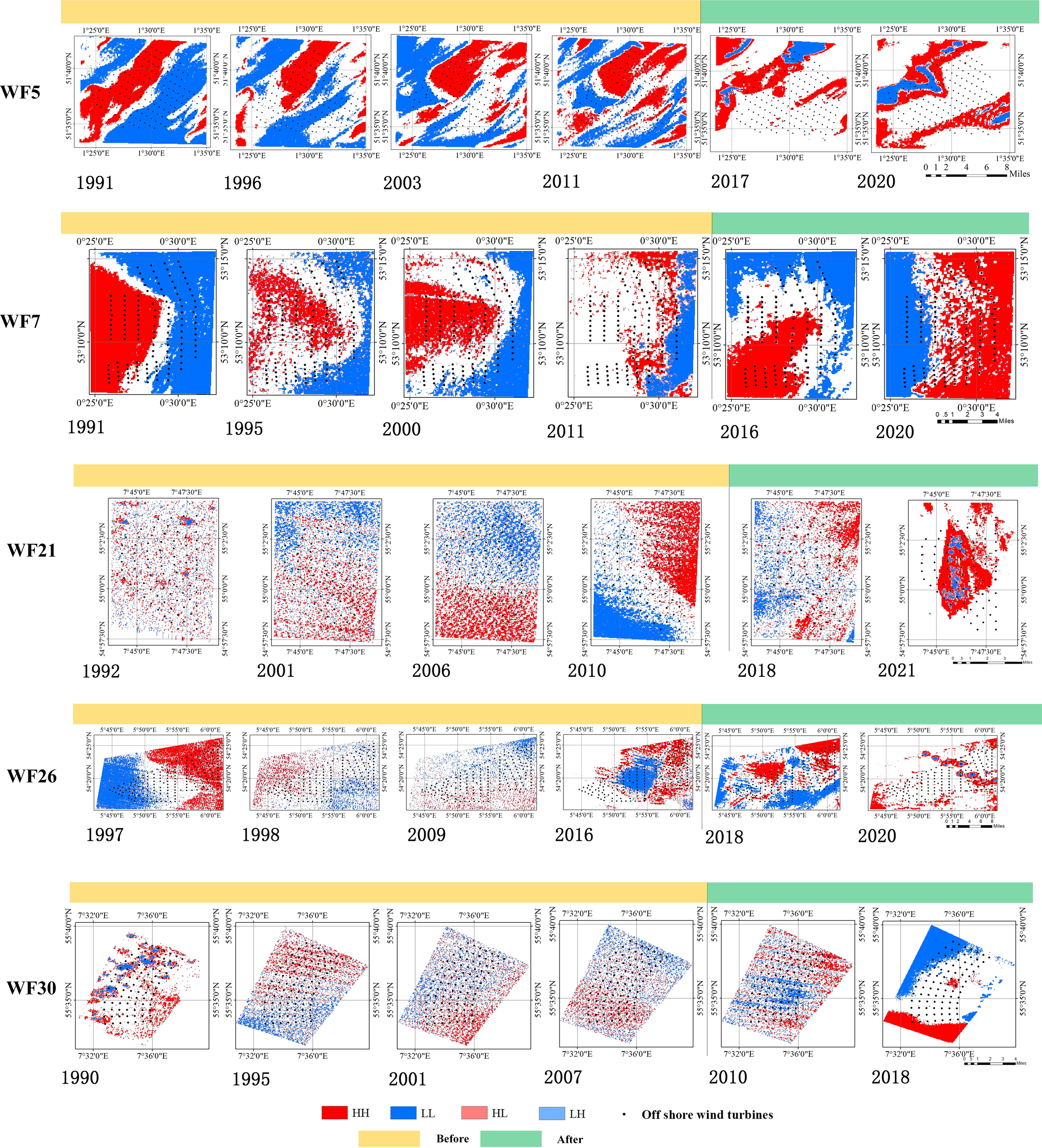
Figure 6 Local Moran’s I with no obvious change areas after OWF construction.

For WF19, WF20, WF21, WF25, WF26, WF27 and WF30, no significant HH or LL Chl-a spatial aggregation after OWF construction was found: the HH and LL picture elements still had decentralized distributions. For WF5, WF7 and WF10, there was greater HH and LL Chl-a spatial aggregation before OWF construction. Even after the construction of WF5, the number of internal HH and LL pixels decreased. This irregular spatial variation of Chl-a concentration indicated that the construction of these OWFs did not cause significant concentrations of HH and LL.

Through the above analysis, the changes in Chl-a concentrations for all OWFs were determined. Across 38 study areas, the spatial distribution pattern of Chl-a concentration at 28 OWFs showed aggregation after the OWF construction, accounting for 73.7% of the total number of OWFs. For the other 10 OWFs, accounting for 26.3% of the total number of OWFs, no significant trends in the spatial distribution patterns of Chl-a concentration were found. Therefore, it was concluded that the construction of OWFs has a certain impact on Chl-a concentration, which is manifest as the aggregation of HH and LL.

Discussion

Reasons for Chl-a aggregation

The global Moran’s I results revealed that the spatial autocorrelation of Chl-a concentration increased after the construction of 37 out of the 38 OWFs. This indicated that the increase in Chl-a spatial autocorrelation was related to OWF construction. The construction of an OWF changed the Chl-a concentration in the region; that is, the phytoplankton in the region was affected. However, the increase in spatial autocorrelation did not mean that the Chl-a concentration had increased or decreased; rather, it was only a reflection of the spatial correlation between concentrations.

The local Moran’s I results revealed that HH and LL Chl-a concentrations occurred. That is, there were both high-concentration Chl-a concentration areas and low-concentration Chl-a concentration areas near the OWFs. It is thought that an increase in Chl-a concentration is due to an increase in the mean photosynthetic active radiation underwater and a decrease in nutrient concentration, resulting in pronounced eutrophication (McQuatters-Gollop et al., 2007; Alvarez-Fernandez and Riegman, 2014). Studies have also shown that the hard substrate of the OWT attracts many benthic organisms, turning the area into their habitat. This in turn causes local changes in phytoplankton—such as algae—in the seawater (Gill et al., 2018; Michaelis et al., 2019; Voet et al., 2022) and changes the spatial distribution pattern of Chl-a in the area. Additionally, the eddy currents generated during the operation of the turbines in the OWFs cause an increase in the turbulence in the upper and middle seawater layers, which leads to the upwelling of nutrients and phytoplankton in the seawater and finally results in significant discontinuous changes in the phytoplankton concentration in the vicinity of the OWFs (Floeter et al., 2015). This effect is also related to the size of the OWTs (Tweddle et al., 2016). The aggregation of HH Chl-a concentrations may be because phytoplankton, such as algae, cover individual OWFs (Pedersen et al.), or due to the increase of phytoplankton upwelling in the thermocline. The reason for LL aggregation is the gathering of fish and shellfish near OWFs. The aggregation of these marine predators, which feed on phytoplankton, results in a decrease in the Chl-a concentration, but this often occurs in a small-scale spatial range (Wilhelmsson and Malm, 2008; Krone et al., 2013). In the present study, the Chl-a concentration in the vicinity of the OWFs did not simply increase or decrease but showed high-value and low-value aggregation in the spatial distribution. Therefore, this effect needs further study.

According to the results of the present study, before and after the construction of the OWFs in 10 regions, there was no identifiable trend in the spatial distribution of Chl-a within the region. Of these OWFs, WF19, WF20, WF21, WF25, WF26 and WF30 are in the southeast of the North Sea in Europe. From the research results on the spatial-temporal evolution trend of Chl-a in the North Atlantic Ocean, it is possible that the evolution trend in offshore Chl-a may be affected by ocean currents and become part of multi-decade changes. As these OWFs are far offshore compared to other OWFs, they are more likely to be affected by the North Atlantic Ocean currents (Queste et al., 2013; Zhang et al., 2018).

In addition, the region with no obvious trend in the spatial distribution in this study coincided with low PH areas in the North Sea, which resulted in a decrease in phytoplankton and a decrease in Chl-a concentration (Artioli et al., 2012). Low Chl-a concentrations combined with significant changes in ocean currents resulting in no significant accumulation of Chl-a in the spatial distribution pattern in the above regions.

Impacts of OWFs on marine ecosystems

The number of OWFs around the world is increasing. To reduce carbon emissions and make efficient use of wind energy, a clean energy source, the global development of offshore wind power technology is rapidly progressing. But the development of offshore wind power will bring certain ecological impacts. In this paper, the marine environment is evaluated by using the Chl-a retrieved from remote sensing images. this method is of great significance to the ecosystem value (Wang et al., 2021), coastal ecological change (Chen et al., 2022), land use monitoring (Chen et al., 2021), and so on.The results of this study revealed that the construction of OWFs caused HH and LL spatial concentrations of Chl-a. This indicated that the OWFs affected the distribution of phytoplankton, with areas of increased phytoplankton biomass aggregation (HH) and areas of decreased phytoplankton biomass aggregation (LL). Because of this aggregation of phytoplankton near OWFs, the feasibility of the co-location of OWFs and aquaculture has been explored via numerous studies. This approach is based on the belief that the co-location of aquaculture with OWFs would consume increased Chl-a concentrations (Pogoda et al., 2011; Jansen et al., 2016; von Thenen et al., 2020) and provide a mutually beneficial solution with positive impacts on the marine ecosystem.

Conclusion

The development of offshore wind energy contributes to goals such as saving energy and reducing carbon emissions. However, as thousands of offshore wind turbines enter the oceans, determining their ecological impact is also important. In this study, changes in the concentration of Chl-a—which is closely related to the marine ecosystem—were selected to determine the impact of the construction of OWFs on the marine ecological environment. Through a comparative analysis of the spatial distribution pattern and spatial autocorrelation of Chl-a before and after the construction of OWFs, it was found that the OWFs resulted in a concentration of the spatial distribution pattern of Chl-a and the co-occurrence of HH and LL concentrations in each OWF area. These results indicated that there were increased and decreased risks relating to the concentration of seawater Chl-a arising from the construction of OWFs.

With the booming development of offshore wind power, not only will many OWTs enter the sea in the future but the decommissioning and dismantling of OWTs will also occur. Minimizing the negative impact of the construction and dismantling of OWTs on the marine ecological environment is of great significance for the sustainable development of offshore wind power. Determining the spatial variation of Chl-a could provide insights into the impacts of the development of offshore wind power in the future and be conducive to designing and formulating a reasonable installation or removal plan to obtain the optimal environmental effect.

Data availability statement

The raw data supporting the conclusions of this article will be made available by the authors, without undue reservation.

Author contributions

LuZ:Writing – original draft, Data curation, Methodology, Formal analysis. LG:Conceptualization, Supervision, Methodology, Writing –review & editing, Conceptualization, Formal analysis. LiZ:Writing - Review & editing, Data curation. WL:Writing - Review & editing, Data curation. All authors contributed to the article and approved the submitted version.

Funding

This research received financial support from the National Natural Science Fund of China(42271266,42071385), the National Natural Science Fund of Shandong Province (ZR2021MD051), Yantai Science and Technology Innovation Development Plan Project(2022MSGY062), the Open Project Program of Shandong Marine Aerospace Equipment Technological Innovation Center, Ludong University(Grant No.MAETIC2021-12).

Conflict of interest

The authors declare that the research was conducted in the absence of any commercial or financial relationships that could be construed as a potential conflict of interest.

Publisher's note

All claims expressed in this article are solely those of the authors and do not necessarily represent those of their affiliated organizations, or those of the publisher, the editors and the reviewers. Any product that may be evaluated in this article, or claim that may be made by its manufacturer, is not guaranteed or endorsed by the publisher.

References

Alvarez-Fernandez S., Riegman R. (2014). Chlorophyll in north Sea coastal and offshore waters does not reflect long term trends of phytoplankton biomass. J. Sea Res. 91, 35–44. doi: 10.1016/j.seares.2014.04.005

CrossRef Full Text | Google Scholar

Andersson M. H. (2011). Offshore wind farms-ecological effects of noise and habitat alteration on fish (Stockholm University: Department of Zoology).

Google Scholar

Anselin L. (1995). Local indicators of spatial association–LISA. Geographical Anal. 27 (2), 93–115. doi: 10.1111/j.1538-4632.1995.tb00338.x

CrossRef Full Text | Google Scholar

Anselin L. (2019). “The Moran scatterplot as an ESDA tool to assess local instability in spatial association,” in Spatial analytical perspectives on GIS (England: Routledge) 111–126.

Google Scholar

Artioli Y., Blackford J. C., Butenschön M., Holt J. T., Wakelin S. L., Thomas H., et al. (2012). The carbonate system in the north Sea: Sensitivity and model validation. J. Mar. Syst. 102-104, 1–13. doi: 10.1016/j.jmarsys.2012.04.006

CrossRef Full Text | Google Scholar

Benassai G., Mariani P., Stenberg C., Christoffersen M. (2014). A sustainability index of potential co-location of offshore wind farms and open water aquaculture. Ocean Coast. Manage. 95, 213–218. doi: 10.1016/j.ocecoaman.2014.04.007

CrossRef Full Text | Google Scholar

Brewin R. J. W., Dall'Olmo G., Pardo S., van Dongen-Vogels V., Boss E. S. (2016). Underway spectrophotometry along the Atlantic meridional transect reveals high performance in satellite chlorophyll retrievals. Remote Sens. Environ. 183, 82–97. doi: 10.1016/j.rse.2016.05.005

CrossRef Full Text | Google Scholar

Brewin R. J. W., Raitsos D. E., Pradhan Y., Hoteit I. (2013). Comparison of chlorophyll in the red Sea derived from MODIS-aqua and in vivo fluorescence. Remote Sens. Environ. 136, 218–224. doi: 10.1016/j.rse.2013.04.018

CrossRef Full Text | Google Scholar

Callbeck C. M., Ehrenfels B., Baumann K. B., Wehrli B., Schubert C. J. (2021). Anoxic chlorophyll maximum enhances local organic matter remineralization and nitrogen loss in lake Tanganyika. Nat. Commun. 12 (1), 1–11. doi: 10.1038/s41467-021-21115-5

PubMed Abstract | CrossRef Full Text | Google Scholar

Chen H., Chen C., Zhang Z., Lu C., Wang L., He X., et al. (2021). Changes of the spatial and temporal characteristics of land-use landscape patterns using multi-temporal landsat satellite data: A case study of zhoushan island, China. Ocean Coast. Manage. 213, 105842. doi: 10.1016/j.ocecoaman.2021.105842

CrossRef Full Text | Google Scholar

Chen C., Liang J., Xie F., Hu Z., Sun W., Yang G., et al. (2022). Temporal and spatial variation of coastline using remote sensing images for zhoushan archipelago, China. Int. J. Appl. Earth Observation Geoinformation 107, 102711. doi: 10.1016/j.jag.2022.102711

CrossRef Full Text | Google Scholar

Coates D. A., Deschutter Y., Vincx M., Vanaverbeke J. (2014). Enrichment and shifts in macrobenthic assemblages in an offshore wind farm area in the Belgian part of the north Sea. Mar. Environ. Res. 95, 1–12. doi: 10.1016/j.marenvres.2013.12.008

PubMed Abstract | CrossRef Full Text | Google Scholar

De Borger E., Ivanov E., Capet A., Braeckman U., Vanaverbeke J., Grégoire M., et al. (2021). Offshore windfarm footprint of sediment organic matter mineralization processes. Front. Mar. Sci. 8. doi: 10.3389/fmars.2021.632243

PubMed Abstract | CrossRef Full Text | Google Scholar

Degraer S., Carey D. A., Coolen J. W., Hutchison Z. L., Kerckhof F., Rumes B., et al. (2020). Offshore wind farm artificial reefs affect ecosystem structure and functioning. Oceanography 33 (4), 48–57. doi: 10.5670/oceanog.2020.405

CrossRef Full Text | Google Scholar

Díaz H., Guedes Soares C. (2020). Review of the current status, technology and future trends of offshore wind farms. Ocean Eng. 209, 107381. doi: 10.1016/j.oceaneng.2020.107381

CrossRef Full Text | Google Scholar

Fishman T., Graedel T. (2019). Impact of the establishment of US offshore wind power on neodymium flows. Nat. Sustainability 2 (4), 332–338. doi: 10.1038/s41893-019-0252-z

CrossRef Full Text | Google Scholar

Floeter J., Callies U., Dudeck T., Eckhardt A., Gloe D., Hufnagl M., et al. (2015). “Assessing bio-physical effects of offshore wind farms on the north Sea pelagic ecosystem using a TRIAXUS ROTV,” in EGU General Assembly Conference Abstracts, 4082. (Vienna, Austria:EGU General Assembly 2015).

Google Scholar

Floeter J., van Beusekom J. E. E., Auch D., Callies U., Carpenter J., Dudeck T., et al. (2017). Pelagic effects of offshore wind farm foundations in the stratified north Sea. Prog. Oceanography 156, 154–173. doi: 10.1016/j.pocean.2017.07.003

CrossRef Full Text | Google Scholar

Furness R. W., Wade H. M., Masden E. A. (2013). Assessing vulnerability of marine bird populations to offshore wind farms. J. Environ. Manage. 119, 56–66. doi: 10.1016/j.jenvman.2013.01.025

PubMed Abstract | CrossRef Full Text | Google Scholar

Gill A., Birchenough S., Jones A., Judd A., Jude S., Payo A., et al. (2018). Implications for the marine environment of energy extraction in the sea (England:Routledge Taylor and Francis Group London and New York).

Google Scholar

Hu C. (2011). An empirical approach to derive MODIS ocean color patterns under severe sun glint. Geophysical Res. Lett. 38 (1), L01603. doi: 10.1029/2010GL045422

CrossRef Full Text | Google Scholar

Hu C., Lee Z., Franz B. (2012). Chlorophyll aalgorithms for oligotrophic oceans: A novel approach based on three-band reflectance difference. J. Geophysical Research: Oceans 117 (C1), C01011. doi: 10.1029/2011JC007395

CrossRef Full Text | Google Scholar

Jansen H. M., Van Den Burg S., Bolman B., Jak R. G., Kamermans P., Poelman M., et al. (2016). The feasibility of offshore aquaculture and its potential for multi-use in the north Sea. Aquaculture Int. 24 (3), 735–756. doi: 10.1007/s10499-016-9987-y

CrossRef Full Text | Google Scholar

Kamermans P., Walles B., Kraan M., Van Duren L. A., Kleissen F., van der Have T. M., et al. (2018). Offshore wind farms as potential locations for flat oyster (Ostrea edulis) restoration in the Dutch north Sea. Sustainability (Switzerland) 10, 308. doi: 10.3390/su10113942

CrossRef Full Text | Google Scholar

Khosravi Y., Bahri A., Tavakoli A. (2018). Spectral analysis of spatial relationship between surface wind speed (SWS) and Sea surface temperature (SST) in Oman Sea. Phys. Geogr. Res. Q. 50 (3), 473–489. doi: 10.22059/JPHGR.2018.245219.1007137

CrossRef Full Text | Google Scholar

Krone R., Gutow L., Joschko T. J., Schröder A. (2013). Epifauna dynamics at an offshore foundation – implications of future wind power farming in the north Sea. Mar. Environ. Res. 85, 1–12. doi: 10.1016/j.marenvres.2012.12.004

PubMed Abstract | CrossRef Full Text | Google Scholar

Li Z., Tian G., El-Shafay A. S. (2022). Statistical-analytical study on world development trend in offshore wind energy production capacity focusing on great Britain with the aim of MCDA based offshore wind farm siting. J. Cleaner Production 363, 132326. doi: 10.1016/j.jclepro.2022.132326

CrossRef Full Text | Google Scholar

Mavraki N., Degraer S., Vanaverbeke J., Braeckman U. (2020). Organic matter assimilation by hard substrate fauna in an offshore wind farm area: a pulse-chase study. ICES J. Mar. Sci. 77 (7-8), 2681–2693. doi: 10.1093/icesjms/fsaa133

CrossRef Full Text | Google Scholar

McQuatters-Gollop A., Raitsos D. E., Edwards M., Pradhan Y., Mee L. D., Lavender S. J., et al. (2007). A long-term chlorophyll dataset reveals regime shift in north Sea phytoplankton biomass unconnected to nutrient levels. Limnology Oceanography 52 (2), 635–648. doi: 10.4319/lo.2007.52.2.0635

CrossRef Full Text | Google Scholar

Methratta E. T., Dardick W. R. (2019). Meta-analysis of finfish abundance at offshore wind farms. Rev. Fisheries Sci. Aquaculture 27 (2), 242–260. doi: 10.1080/23308249.2019.1584601

CrossRef Full Text | Google Scholar

Michaelis R., Hass H. C., Mielck F., Papenmeier S., Sander L., Gutow L., et al. (2019). Epibenthic assemblages of hard-substrate habitats in the German bight (south-eastern north Sea) described using drift videos. Continental Shelf Res. 175, 30–41. doi: 10.1016/j.csr.2019.01.011

CrossRef Full Text | Google Scholar

Moran P. A. P. (1950). Notes on continuous stochastic phenomena. Biometrika 37 (1/2), 17–23. doi: 10.2307/2332142

PubMed Abstract | CrossRef Full Text | Google Scholar

Oh H.-T., Chung Y., Jeon G., Shim J. (2021). Review of the marine environmental impact assessment reports regarding offshore wind farm. Fisheries Aquat. Sci. 24 (11), 341–350. doi: 10.47853/FAS.2021.e33

CrossRef Full Text | Google Scholar

O’Reilly J. E., Maritorena S., Siegel D. A., O’Brien M. C., Toole D., Mitchell B. G., et al. (2000). Ocean color chlorophyll a algorithms for SeaWiFS, OC2, and OC4: Version 4. SeaWiFS postlaunch calibration validation analyses Part 3, 9–23. Available at:https://www.academia.edu/10355556/Ocean_color_chlorophyll_a_algorithms_for_SeaWiFS_OC2_and_OC4_Version_4?auto=citations&from=cover_page.

Google Scholar

Pedersen J., Leonhard S. B., Klaustrup M., Hvidt C. B.. (2006) Benthic communities at horns rev before, during and after con-struction of horns rev offshore wind farm (Spain:TETHYS).

Google Scholar

Pogoda B., Buck B. H., Hagen W. (2011). Growth performance and condition of oysters (Crassostrea gigas and ostrea edulis) farmed in an offshore environment (North Sea, Germany). Aquaculture 319 (3), 484–492. doi: 10.1016/j.aquaculture.2011.07.017

CrossRef Full Text | Google Scholar

Pollock C. J., Lane J. V., Buckingham L., Garthe S., Jeavons R., Furness R. W., et al. (2021). Risks to different populations and age classes of gannets from impacts of offshore wind farms in the southern north Sea. Mar. Environ. Res. 171, 105457. doi: 10.1016/j.marenvres.2021.105457

PubMed Abstract | CrossRef Full Text | Google Scholar

Pryor S. C., Barthelmie R. J., Bukovsky M. S., Leung L. R., Sakaguchi K. (2020). Climate change impacts on wind power generation. Nat. Rev. Earth Environ. 1 (12), 627–643. doi: 10.1038/s43017-020-0101-7

CrossRef Full Text | Google Scholar

Queste B. Y., Fernand L., Jickells T. D., Heywood K. J. (2013). Spatial extent and historical context of north Sea oxygen depletion in august 2010. Biogeochemistry 113 (1), 53–68. doi: 10.1007/s10533-012-9729-9

PubMed Abstract | CrossRef Full Text | Google Scholar

Raoux A., Tecchio S., Pezy J.-P., Lassalle G., Degraer S., Wilhelmsson D., et al. (2017). Benthic and fish aggregation inside an offshore wind farm: Which effects on the trophic web functioning? Ecol. Indic. 72, 33–46. doi: 10.1016/j.ecolind.2016.07.037

CrossRef Full Text | Google Scholar

Seegers B. N., Stumpf R. P., Schaeffer B. A., Loftin K. A., Werdell P. J. (2018). Performance metrics for the assessment of satellite data products: an ocean color case study. Optics Express 26 (6), 7404–7422. doi: 10.1364/OE.26.007404

PubMed Abstract | CrossRef Full Text | Google Scholar

Tricas T., Gill A. B. (2011). Effects of EMFs from undersea power cables on elasmobranchs and other marine species (U.S:Bureau of Ocean Energy Management).

Google Scholar

Tweddle J. F., Murray R., Gubbins M., Scott B. E. (2016). Do offshore wind farms influence marine primary production? Am. Geophysical Union 2016, HI51A–HI506. Available at:https://hdl.handle.net/20.500.12594/11211.

Google Scholar

Van Berkel J., Burchard H., Christensen A., Mortensen L. O., Petersen O. S., Thomsen F. (2020). The effects of offshore wind farms on hydrodynamics and implications for fishes. Oceanography 33 (4), 108–117. doi: 10.5670/oceanog.2020.410

CrossRef Full Text | Google Scholar

Voet H. E. E., Van Colen C., Vanaverbeke J. (2022). Climate change effects on the ecophysiology and ecological functioning of an offshore wind farm artificial hard substrate community. Sci. Total Environ. 810, 152194. doi: 10.1016/j.scitotenv.2021.152194

PubMed Abstract | CrossRef Full Text | Google Scholar

Von Thenen M., Maar M., Hansen H. S., Friedland R., Schiele K. S. (2020). Applying a combined geospatial and farm scale model to identify suitable locations for mussel farming. Mar. pollut. Bull. 156, 111254. doi: 10.1016/j.marpolbul.2020.111254

PubMed Abstract | CrossRef Full Text | Google Scholar

Wang L., Chen C., Xie F., Hu Z., Zhang Z., Chen H., et al. (2021). Estimation of the value of regional ecosystem services of an archipelago using satellite remote sensing technology: A case study of zhoushan archipelago, China. Int. J. Appl. Earth Observation Geoinformation 105, 102616. doi: 10.1016/j.jag.2021.102616

CrossRef Full Text | Google Scholar

Wang M., Son S. (2016). VIIRS-derived chlorophyll-a using the ocean color index method. Remote Sens. Environ. 182, 141–149. doi: 10.1016/j.rse.2016.05.001

CrossRef Full Text | Google Scholar

Wang L., Xu M., Liu Y., Liu H., Beck R., Reif M., et al. (2020). Mapping freshwater chlorophyll-a concentrations at a regional scale integrating multi-sensor satellite observations with Google earth engine. Remote Sens. 12 (20), 3278. doi: 10.3390/rs12203278

CrossRef Full Text | Google Scholar

Wilhelmsson D., Malm T. (2008). Fouling assemblages on offshore wind power plants and adjacent substrata. Estuarine Coast. Shelf Sci. 79 (3), 459–466. doi: 10.1016/j.ecss.2008.04.020

CrossRef Full Text | Google Scholar

Zhang T., Tian B., Sengupta D., Zhang L., Si Y. (2021). Global offshore wind turbine dataset. Sci. Data 8 (1), 191. doi: 10.1038/s41597-021-00982-z

PubMed Abstract | CrossRef Full Text | Google Scholar

Zhang M., Zhang Y., Shu Q., Zhao C., Wang G., Wu Z., et al. (2018). Spatiotemporal evolution of the chlorophyll a trend in the north Atlantic ocean. Sci. Total Environ. 612, 1141–1148. doi: 10.1016/j.scitotenv.2017.08.303

PubMed Abstract | CrossRef Full Text | Google Scholar

Zhang C., Zhou H., Cui Y., Wang C., Li Y., Zhang D. (2019). Microplastics in offshore sediment in the yellow Sea and east China Sea, China. Environ. pollut. 244, 827–833. doi: 10.1016/j.envpol.2018.10.102

PubMed Abstract | CrossRef Full Text | Google Scholar