 Najeem Shajahan
 David R Barclay
 Ying-Tsong Lin
- 1Department of Oceanography, Dalhousie University, Halifax, NS, Canada
- 2Applied Ocean Physics and Engineering Department, Woods Hole Oceanographic Institution, Woods Hole, MA, United States
The performance of a hydrophone array can be evaluated by its coherent gain, which depends on the spatial correlation of both the signal of interest and the background noise between different array elements, where one hopes to maximize the former while minimizing the latter with array signal processing. In this paper, a computational vertical noise coherence map of the first zero-crossing is generated near Alvin Canyon, south of Martha’s Vineyard, Massachusetts, to study its dependence on the spatial variation in bathymetry, water column sound speed and sediment type. A two and three-dimensional Parabolic Equation propagation model based on reciprocity theory were used for the simulation. The results showed that the seabed parameters have the greatest impact on vertical noise coherence at the array location in the Alvin Canyon area, when compared to 3-D bathymetric and water column sound speed profile variability, especially in the shallower water. The analysis reveals the ideal spacing for a vertical hydrophone array for better signal detection in acoustic experiments. In the continental shelf and slope regions, the ideal spacing lies between 3λ⁄8 in deep water and λ⁄2 in shallow water, and for areas with strong bathymetric variations the ideal spacing can be determined by comprehensive numerical models.
1 Introduction
Signal detection in a poorly characterized and noisy ocean environment is a challenging problem. Hydrophone arrays are commonly used to improve signal detection against background ambient noise. They are used in active and passive SONAR, transmission loss (TL) experiments, seismic operations, and a variety of passive acoustic monitoring applications. The performance of an array can be evaluated by its array gain (AG) which is the improvement in signal-to-noise ratio (SNR) of the array relative to a single sensor, or the difference between signal gain (SG) and noise gain (NG) in dB (Urick, 1967). The response of the array to noise is expressed in NG which depends on the spatial characteristics of ambient noise field (Buckingham, 1981). Thus, the spatial coherence of ambient noise is directly related to the AG.
Analysis of the space-time correlation property of ambient noise received on an array provides the spatial coherence. It is a normalized quantity dependent on the ocean environmental properties and the type of noise source. Typically, the sources of ambient noise in the ocean can be broadly classified as natural and man-made (Wenz, 1962). Wind-induced breaking wave, rain fall, and biological sources are the common sources of natural ambient noise. Ship traffic, sonar operations, and offshore exploration and constructions are the prominent sources of man-made noise in the ocean. Among these sources, the wind-generated sound is omnipresent and the primary contributor to ambient noise in the ocean. Because of the random nature of the signals generated at the ocean surface, the prediction of noise field requires detailed knowledge of the properties of the sound propagation environment. Many of the measurement and modelling studies of spatial coherence are location specific and used as a tool for noise-based inversion of the ocean environment (Buckingham, 1979; Hamson, 1980; Buckingham and Jones, 1987; Carbone et al., 1998; Muzi et al., 2016; Shajahan et al., 2020).
The two familiar models of spatial coherence are the isotropic and the surface noise models developed by Cron and Sherman (Cron and Sherman, 1962). The isotropic model considers the noise field as statistically independent plane waves propagating in all directions uniformly while the surface noise model assumes sources to be distributed on an infinite plane just below the surface of the ocean. Although the surface noise model agrees well with deep water measurements (Barclay and Buckingham, 2013a; Barclay and Buckingham, 2013b), the model does not include sound propagation characteristics such as refraction, attenuation, and boundary reflections. Kuperman-Ingenito introduced a noise model for spatial coherence in a stratified media by considering noise sources as monopoles distributed just below the ocean surface (Kuperman and Ingenito, 1980). Buckingham similarly presented an analytical solution for the vertical coherence of surface-generated noise applicable in an isovelocity shallow water waveguide (Buckingham, 1980). A simple closed-form solution for vertical coherence based on ray theory was developed by Harrison and found to be very effective in noise-based inversion applications (Harrison, 1996). These models are all capable of computing the stationary second order statistics of the noise field under various simplifying assumptions, among the most pronounced are an axially-symmetric and range-independent bathymetry and sound speed profile. Carey introduced a computational theory for noise spatial correlation and directionality by simulating a single snapshot of the pressure field at the sensors using a PE propagation model with randomly distributed noise sources (Carey et al., 1990; Carey and Evans, 2011)
Knowledge of the mesoscale spatial variation of vertical coherence and the relative influence of environmental factors is required for the design of element spacing of arrays or conversely, predicting array performance. However, the isotropic and surface noise models have difficulty modelling the continental shelf and slope regions, especially around strong bathymetric features such as submarine canyons. Also, the properties of the waveguide can affect noise propagation causing anisotropy in the noise field and the spatial coherence. Accurate fine-scale spatial measurements (resolution 10’s of km2) of vertical noise coherence over a large area are difficult to obtain due to high experimental effort and cost to make the acoustic measurement while also characterizing the ocean environment. This motivates a need for predictive models of noise coherence. Besides that, modelling the spatial properties of noise, both the spatial variability and spatial correlations is a useful prerequisite for the successful execution of active and passive acoustic experiments and operations. Predictions of noise correlation may be used to inform sonar array design (e.g. receive element spacing and operating frequency) while knowledge of spatial variability may be used to optimally choose the array location.
In this paper, a map of the vertical coherence of ambient noise is generated showing its first zero-crossing, and its dependence on environmental factors is analyzed on spatial scales greater than 100 km2. The study region was chosen around Alvin Canyon, south of Martha’s Vineyard, Massachusetts. A PE sound propagation model based on reciprocity theory was used for the simulation of the noise field (Barclay and Lin, 2019). The simulation results will provide a quantitative estimate AG relative to different sound propagation conditions and model configurations. The rest of the manuscript is organized as follows: Section 2 presents the basic theory of spatial coherence and AG. Section 3 shows the method for modelling ambient noise using a 3-D PE model and the description of the environmental inputs used in the simulation. In section 4, the simulation results of vertical coherence and array gain for different test cases are described. Finally, the conclusions based on the analysis are given in section 5.
2 Theory- array gain and vertical coherence
The array gain is determined using the following simple relationship,
where SG and NG are reported in dB. The AG of a linear array with discrete hydrophones can be expressed in terms of cross-correlation coefficient as
where ΓS is the correlation coefficient of the signal, ΓN is the correlation coefficient of the noise field, and n and m are the indices of the sensors along the array. When the noise is incoherent and the signal has a unit correlation between array elements, the array performance increases logarithmically with the number of hydrophones. When the noise is partially coherent, the array performance degrades depending on the coherence of noise signals. The overall array performance in general depends on the degree of coherence existing between noise signals received at different hydrophones across the array.
Two common reference models of spatial coherence are used to describe noise coherence with closed form expressions. The isotropic model considers the superposition of plane waves uniformly distributed over all directions. The normalized correlation function for the isotropic noise model can be expressed as a sinc function:
where k is the wavenumber and d is the spacing between array elements, independent of the orientation.
The surface noise model developed by Cron-Sherman is more realistic compared to the isotropic noise model and is primarily used for deep-water applications. The model assumes only downward travelling noise in a semi-infinite, non-attenuating, homogeneous half-space ocean with azimuthal symmetry. Based on the above assumptions, the vertical noise coherence function can be expressed in the closed form expression (Buckingham, 2013)
According to Cox, in a homogeneous noise field, the real part of coherence for surface-generated noise represents the symmetry in the noise field about the horizontal while the imaginary part represents the asymmetry (Cox, 1973). The real (blue solid line) and imaginary (blue dashed line) components of coherence for an isotropic noise field as a function of the ratio between hydrophone spacing and wavelength (d⁄λ) are shown in Figure 1. The real part of coherence falls to zero at half-wavelength spacings (λ⁄2). If we use isotropic assumption in Eq. 2 with λ⁄2 spacing for an array, AG increases logarithmically with the number of hydrophones. The imaginary part of the isotropic noise model is zero due to the symmetry in the noise field.
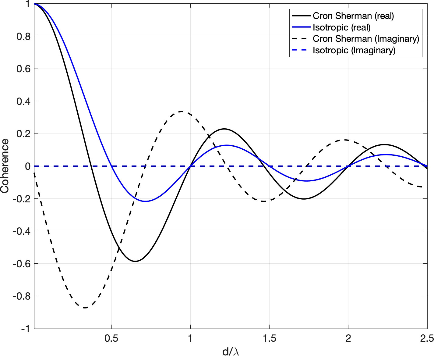
Figure 1 The real and imaginary vertical noise coherence according to the isotropic and Cron-Sherman models. Buckingham, M. J. (2013).
The real (black solid line) and imaginary (black dashed line) component of coherence for the Cron-Sherman model are also shown in Figure 1. The complex coherence function given in Eq. 4 shows the anisotropic nature of noise directionality. In general, the coherence is higher for Cron-Sherman model, especially at the first λ⁄2 spacing. When the signal coherence is constant, this increase in noise coherence may cause a degradation in the AG compared to the prediction made using isotropic noise field model. Thus, the position of the first zero-crossing of the real part of coherence is a critical parameter in designing the spacing between sensors for sonar applications.
The position of the first zero-crossing can vary depending on the sound speed profile, sediment type, bathymetry, and horizontally propagating distant sound in the measurement location (Buckingham and Jones, 1987; Carbone et al., 1998; Shajahan et al., 2020). The environmental influence on the noise coherence can be analyzed by mapping the first zero-crossing in space. In this work, the position of the first zero-crossing of the Cron-Sherman model is used as a canonical deep-water reference and where the relative departure from this spacing for different cases is mapped and investigated.
3 Mapping ambient noise vertical coherence
3.1 Three-dimensional ambient noise field modelling
The ambient noise field can be considered as a superposition of pressure fields due to individual sources. Normally, for wind-generated noise, the sources are assumed to be distributed just below the surface with a specific source intensity per unit area. Common analytical noise models consider a statistical distribution of individual sources and the cross-spectral density for a range-independent environment is obtained by integrating over range and azimuth (Harrison,1996; Cron and Sherman, 1962; Buckingham, 1980). An alternate approach adapted here is to use a sound propagation model to calculate the pressure field from surface distributed sources. The parabolic-equation (PE) approximation of the full wave equation is a convenient way to determine the acoustic field due to distant sources in a range-dependent environment (Tappert, 1974). In this case, the PE model exploits the principle of reciprocity following the acoustic wave Green’s function equation. The pressure field is identical regardless of the direction of propagation between two points, so the positions of sources and receivers may be interchanged for computational convenience. The complex pressure field computed at a receiver depth just below the surface at zs for an omnidirectional source at z1 can be used to determine the received signal at z1 for a layer of sources placed at zs (note the interchanged source and receiver positions). Thus, in the case of wind-generated noise, where the total received field is sum of all the contributions from individual sources in the horizontal plane just below the surface, the noise power at depth z1 in a cylindrical grid (r,β) can be obtained as,
where P(ω,zs(rq,βp)|z1)≡P(ω,z1|zs(rq,βp)) according to the principle of reciprocity and is the complex acoustic Green’s function in the model domain, zs is essentially the noise source depth, ω is the angular frequency, rq=r0+qΔrq is the discretized range of the qth noise source, βp=pΔβ is the bearing of the pth radial, and |σ(rq,βp)2| is the ensemble average of the noise source strength. ΔβΔrrq is the cylindrical coordinate element area over which the noise sources have been integrated. The cross spectral density (CSD) can be computed by placing a second source at depth z2 and combining the two computed fields to yield
where the * denotes the complex conjugate.
A detailed description of the reciprocal PE noise model method has been previously given (Barclay and Lin, 2019). The accuracy of this reciprocal PE noise model has also been validated against benchmark solutions of an analytical noise coherence model in a shallow water Pekeris waveguide and Cron-Sherman formula in deep water (Deane et al., 1997; Barclay and Lin, 2019). By keeping the sources at positions z1 and z2, the complex pressure field can be calculated for the model domain. Once the power spectrum and cross-spectrum are computed, the normalized cross-spectral density, or coherence, can be determined by
An axially independent two-dimensional (Nx2-D) and a 3-D PE model using the split-step Fourier algorithm with a wide-angle PE approximation was used to calculate the pressure fields in this study (Lin et al., 2013; Lin et al., 2015). The 3-D model solves the forward propagating PE equation simplified from the Helmholtz wave equation by neglecting backward propagating energy in a cylindrical coordinate system with a one-way marching algorithm originating from the source position, allowing horizontal propagation between radial marching directions.
3.2 Environmental input parameters
The main input parameters required for the 3-D PE model in this study are spatially varying bathymetry, water column sound speed and seabed sediment geoacoustic properties. The model domain was selected near Alvin Canyon, south of Martha’s vineyard, Massachusetts. This location was chosen due to the characteristics of the acoustic waveguide (vertical and horizontal variability in sound speed and sediment property) and rapidly changing bathymetry. The two major submarine canyons present in the region were the Alvin Canyon at the longitude 70.5°CW and the Atlantis Canyon at 70.25°CW. The bathymetric variations in the model domain were significant to study the 3-D effect (horizontal refraction) of sound propagation on the vertical noise coherence. The water column stratification of the region was also complex due to the presence of shelf break front, warm-core eddies, freshwater influence and internal wave activity (Zhang and Gawarkiewics, 2015). The location contains a large variety of propagation environments such as shallow water with hard and soft sediment, deep water, and complicated shelf break. Moreover, many modern acoustics experiments like SW-06 (Shallow water 06) and SBCEX-2017 (SeaBed Characterization EXperiment) were conducted in the region to understand the effect of complex environment on acoustic propagation (Tang et al., 2007; Barclay et al., 2019; Wilson et al., 2020; Bonnel et al., 2021).
The sediment type of the region was obtained from the US geological survey data base (Reid et al., 2005) Hamilton’s sediment model for the continental slope environment was used to estimate the geoacoustic properties of each sediment sample from the database (Hamilton, 1980; Jensen et al., 2011). Compressional sound speed, density, and bottom loss were estimated and the map of compressional sound speed and bottom loss for the study region is given in Figures 2A, B respectively. The environmental model assumed a planar sea surface with total internal reflection. Bathymetric data, shown in Figure 2C, were drawn from the Global Multi Resolution Topography (GMRT) database with 45 m resolution in latitude and 70 m resolution in longitude (Ryan et al., 2009). The data assimilated Regional Ocean Modeling System (ROMS) Experimental System for Predicting Shelf and Slope Optics (ESPreSSO) model output was used to extract average water temperature and salinity covering the study region (Rutgers Ocean Modelling Group). Sound speed profiles are derived using the Mackenzie equation from temperature and salinity for November 2016 due to the presence of warm core ring in the months of spring and summer (Mackenzie, 1981; Zhang and Gawarkiewics, 2015). The sound speed map at 50 m depth for the model domain is shown in Figure 2D. Below the mixed-layer, most of the grid points followed a downward refracting sound speed profile which is the characteristics of a typical winter profile of the study region. The variation in sound speed as a function of depth from a deep water grid point is shown in Figure 2E.
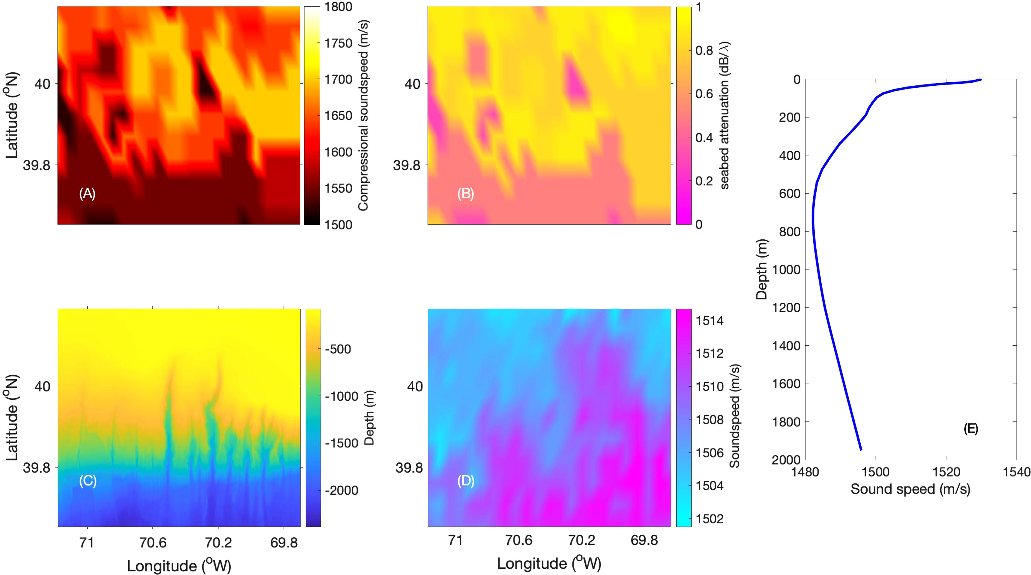
Figure 2 The environmental properties of the model domain (A) seabed compressional sound speed (B) seabed attenuation (C) bathymetry (D) water column sound speed at 50 m depth and (E) a deep water sound speed profile.
4 Results and discussions
The numerical simulations were performed to understand the relative effect of various levels of environmental variability on the vertical noise coherence and noise gain. For computational efficiency, the simulations were performed for a single frequency of 50 Hz over a model grid resolution of 6×6 km, and later the zero-crossing point of the noise coherence will be computed following the dimensionless independent variable d/Λ as depicted in Figure 1. Also, a homogeneous surface generated ambient noise field is assumed (Buckingham, 1980). A vertical array of 40 0-dB model sources with 1 m spacing spanning the water column from 40 to 79 m depths were used to compute the sound pressure just below the sea surface for a horizontal range of 10 km. By invoking the principle of reciprocity, the power spectrum, cross-spectrum and coherence of surface-generated noise between all the elements of the vertical array (originally a source array, but now a receiver array after applying reciprocity) were computed using Eqs. 5, 6, and 7 respectively.
The numerical simulations were carried out for four test cases with different environmental variations. These cases were chosen to study the individual effects of environmental inputs on noise coherence separately. In Case 1, a 2-D PE model was used to simulate noise coherence at every one degree of bearing to generate an N×2-D noise field. The N×2-D environment considers only the bathymetric variation in the radial direction and neglects the transverse variation of the seafloor and any other out-of-vertical-plane sound propagation between radials. The water column sound speed at each grid point was taken as constant for this first case. The dominant component of surficial sediment in the study region was fine sand. Thus, the same geoacoustic properties were used for the seabed at each grid point with a compressional sound speed Cb= 1650m/s, density ρ=1900kg/m3 and attenuation αb =0.8 dB⁄λ.
Case 2 examined the bathymetry induced horizontal refraction by replacing the N×2-D model with a 3-D model with the environmental inputs being the same as in case 1. Case 3 studied the effects caused by the sound speed profile by replacing the constant sound speed in the water column with a local range-independent sound speed c(z). In Case 4, the combined effect of bathymetry, sound speed profile and sediment properties on ambient noise vertical coherence was examined. Table 1 summarizes the four test cases and their respective environmental inputs.
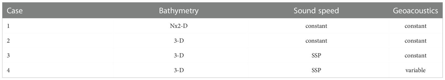
Table 1 Test cases and corresponding environmental input parameters.
The relative change in the first zero-crossing coherence point from the Cron-Sherman model for Cases 1 and 2 and their difference are shown in Figure 3. The bathymetric data of the study domain are shown as isobath contours in each coherence map. Both cases considered constant sound speed in the water column and identical sediment properties at each grid point in the model domain. Thus, this comparison solely focuses on the effect of range-dependent topography. The N×2-D simulation does not include transverse coupling of sound energy across the vertical plane. On the other hand, the 3-D PE model incorporates sound focusing and defocusing due to horizontal refraction. Examination of Figures 3A, B shows that the relative change for Cases 1 and 2 is higher than 50% in shallow water (< 200 m) for both cases. This result clearly suggests the inaccuracy of the Cron-Sherman model in representing the noise field in shallow waters. The proximity of the seabed can introduce interaction of sound with the ocean boundaries resulting in bottom reflected arrivals at the sensors. Moreover, the sandy bottom type used for the simulation may cause horizontal propagation of noise below the critical angle as a result of total internal reflection. Both these factors can contribute to the symmetry in the noise field resulting in an increase in the first zero-crossing coherence point compared to the Cron-Sherman model.
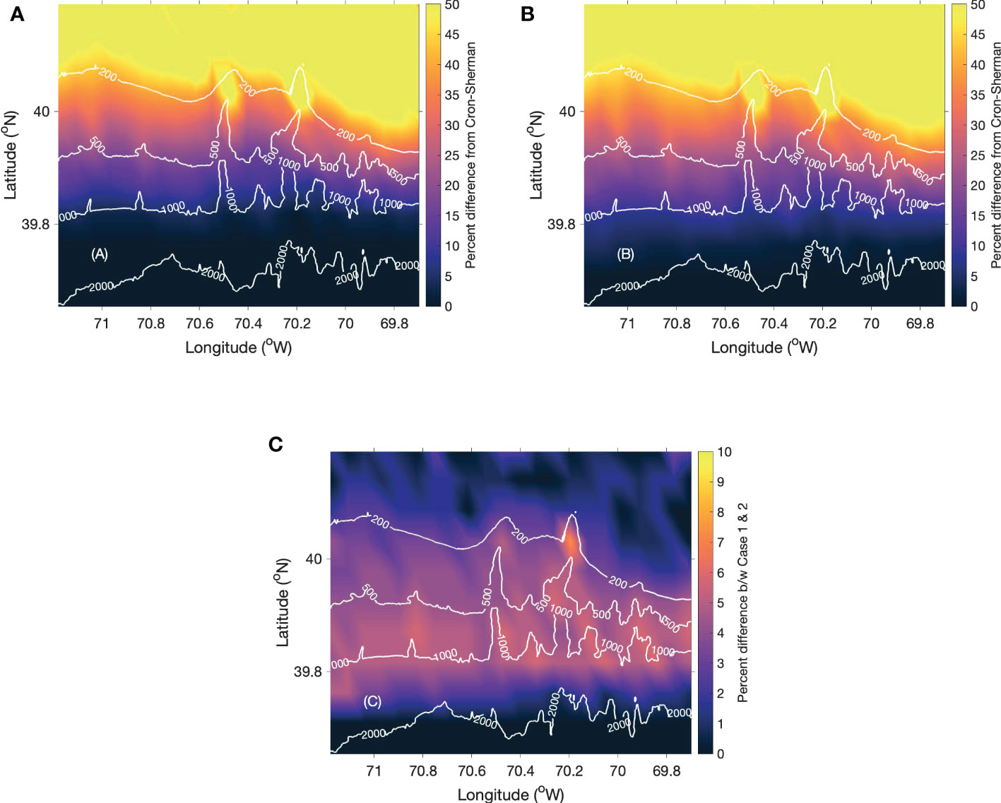
Figure 3 The percentage difference between the Cron-Sherman and computational vertical noise coherence model’s first zero-crossing point for (A) Case 1, (B) Case 2 and (C) the difference between Cases 1 and 2.
The relative change approaches 0% for Case 1 in regions with depth greater than 1000 m. This shows the agreement between the N×2-D simulation and the Cron-Sherman model in deep water regions. However, Case 2 shows a 10-15% increase in zero-crossing coherence point between 1000 and 2000 m while above 2000 m the coherence map agrees well with the surface noise model. The difference between Cases 1 and 2, shown in Figure 3C, shows the importance of 3-D propagation effects in regions of variable bathymetry, especially between the 200 and 2000 m isobaths. The rapidly changing bathymetry in the continental slope regions can induce horizontal refraction and sound focusing resulting in a 10-15% difference between 2-D and 3-D modelling.
The relative change in percentage from the Cron-Sherman model for Cases 2 and 3 are shown in Figures 4A, B respectively. The constant sound speed is replaced by a sound speed profile at each grid point in Case 3. In comparison with Case 2, the shallow water regions of Case 3 showed a decrease in the relative change up to 30%. The first zero-crossing coherence point of the deep-water regions for Case 3 matches with the Cron-Sherman model result. The interaction of sound with the seabed is larger for a downward refracting sound speed profile when compared to a constant sound speed water column. As sound interacts more with the seabed, the increased bottom loss may cause asymmetry in the noise field and most of the energy remains at the surface. As a result, the relative change in shallow waters for Case 3 is less compared to Case 2. The difference between Cases 2 and 3 is shown in Figure 4C. This analysis clearly shows the importance of an accurate sound speed profile in the simulation of the spatial characteristics of ambient noise (Barclay and Buckingham, 2013a; Barclay and Buckingham, 2014).
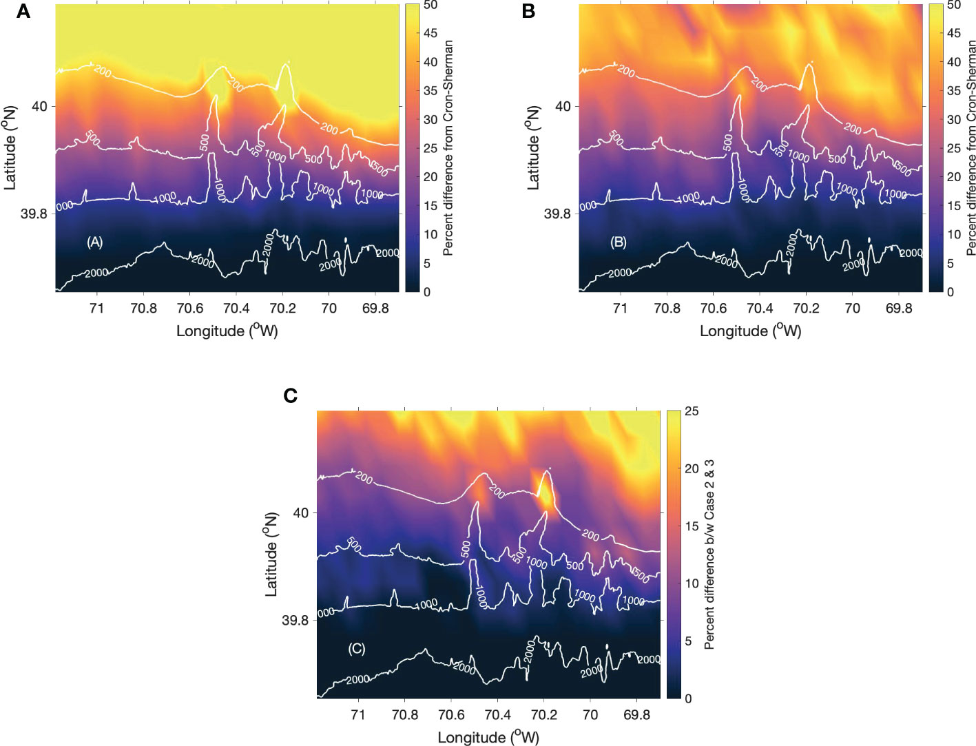
Figure 4 The percentage difference between the Cron-Sherman and computational vertical noise coherence model’s first zero-crossing point for (A) Case 2, (B) Case 3 and (C) the difference between Cases 2 and 3.
In Case 4, all the three spatially varying properties were used to simulate the spatial coherence at each grid point and the noise coherence map was generated using the 3-D propagation model. The relative change for cases 3 and 4 are shown in Figures 5A, B respectively. The noise coherence map of Case 4 is similar to that of case 3 except for some regions in shallow water where the relative change in Case 4 falls to zero as shown in Figure 5B. The map of the sediment compressional sound speed given in Figure 2C indicates that the sediment composition in those regions was clayey silt. Bottom reflection loss mainly depends on the type of sediment. Clayey silt more effectively absorbs the sound energy compared to larger grained sediments. The negative gradient in sound speed profile in shallow water also enhances the interaction with the bottom. As a result, the noise field is dominated by downward travelling sound similar to the assumption of the Cron-Sherman model. Figure 5C shows that the bottom type can cause a difference of up to 40% in the noise coherence map. Identical to the other cases, the noise map for case 4 mostly follows the Cron-Sherman model and the sediment type does not affect the zero-crossing coherent point in deep water. The analysis shows that sediment type is the critical shallow water parameter for an accurate model of the noise field and spatial coherence (Yang and Yoo, 1997; Jensen et al., 2011).
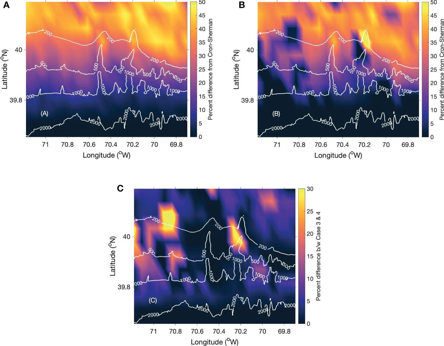
Figure 5 The percentage difference in the first zero-crossing coherence point for (A) Case 3, (B) Case 4 and (C) the difference between Cases 3 and 4.
To demonstrate the influence of spatial variation in environmental properties on signal detection, a map of NG was generated for a 10-element hydrophone array with λ⁄8 spacing coherently summed (with the beam steered broadside). According to Eq. 1, a decrease in NG enhances the overall array performance, while an increase degrades the performance. NG maps were generated using the simulated vertical coherence. Two transects along the latitude as shown in Figure 6 were chosen to study the variation in noise gain from shallow water to deep-water. The first transect (transect a) was away from the canyon axis with a gradually decreasing bathymetry from the continental shelf to deep water. A second transect (transect b) close to the axis of the Alvin canyon was chosen to study the influence of bathymetric variation. The estimated NG of both transects and corresponding bathymetry are shown in Figures 7A, B respectively. NG estimates using the isotropic (black dashed line) and the Cron-Sherman (green dashed line) model are also plotted to compare with the test cases.
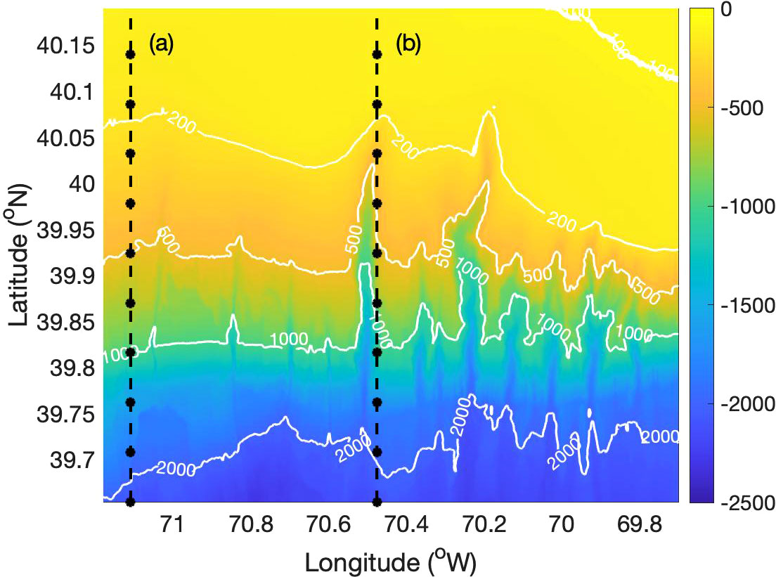
Figure 6 The two transects along latitude (A, B) and the bathymetry of the study region.
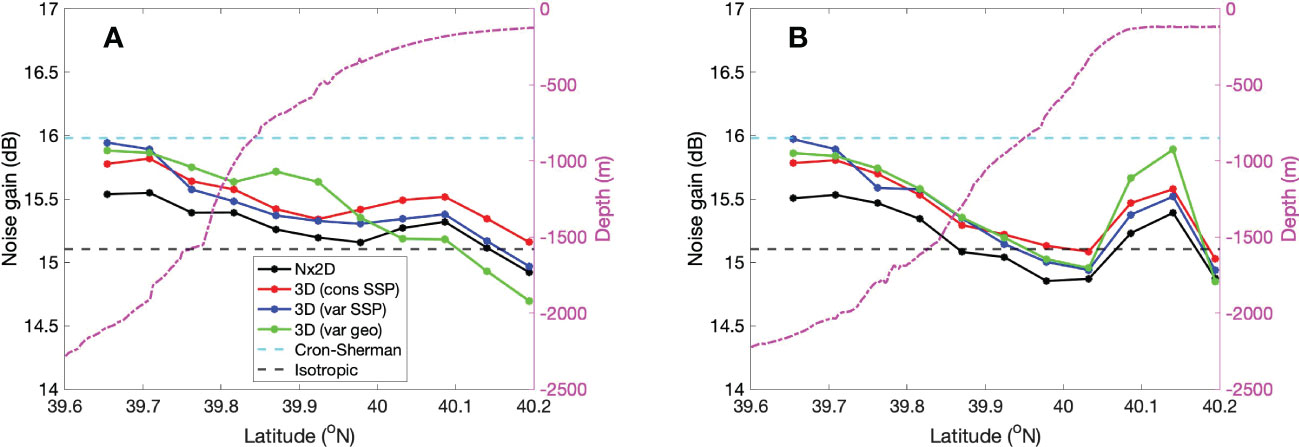
Figure 7 The Noise Gain estimate for a 10-element hydrophone array for (A) transect a and (B) transect b.
In Figure 7A, the NG increases from shallow to deep water in all four test cases. Most of the estimates for transect lie between the isotropic and the Cron-Sherman model with Case 4 showing the largest variation in gain. It can be observed that the NG estimate for test cases in deep water (lower latitude) matches with the Cron-Sherman model and the gain mostly follows the isotropic model in shallow water (higher latitude). The second transect is shown in Figure 7B also followed a similar trend as transect b, except for a slight increase in NG at the head of the canyon. This could be due to the sound focusing caused by changes in the bathymetry at the head.
Lastly, the NG analysis can be used for choosing the ideal spacing of hydrophone arrays for better signal detection in active and passive acoustic experiments by minimizing the NG. Based on the above analysis, it can be inferred that the ideal spacing for a hydrophone array is λ⁄2 in shallow water, which follows the simple isotropic model, and 3λ⁄8 in deep water. However, in regions with varying bathymetry such as continental slope and shelf-break the ideal spacing lies between 3λ⁄8 and λ⁄2 and can be determined by comprehensive numerical models.
5 Conclusions
In sonar performance analysis, AG is a significant factor in determining the signal detection capability. AG not only depends on the coherence of the signal but also on the spatial coherence of ambient noise received between different array elements. Thus, an accurate representation of the ambient noise field is necessary for better signal detection. The simple analytical models of surface-generated noise coherence may not be applicable in complex environments with spatial variation in water column sound speed, bathymetry, geoacoustic properties, and possible 3D propagation effects. Therefore, numerical models can be used in these environments for the accurate representation of the noise field for sonar performance analysis.
In this work, the influence of environment on surface generated ambient noise coherence on a spatial scale of 100 km2 has been analyzed using Nx2-D and 3-D PE models. Range dependent bathymetry, sound speed profile and sediment type were the environmental parameters used for the simulation of the noise field. The four test cases subject to different environmental variability and realism were considered to study the relative influence of waveguide properties on noise coherence. The comparison of noise maps for Nx2-D and 3-D environments showed that the effect of bathymetry induced horizontal refraction is the least compared to the other factors in benign seafloor areas. In shallow water, the sound speed profile is an important factor for accurately representing the noise field. Noise spatial coherence is also found to be more sensitive to seabed acoustic properties in shallow water compared to deep-water regions. Deep water regions are the least affected by the variations in environmental properties. Thus, the Cron-Sherman surface noise model is good enough to represent the spatial coherence in deep water. Furthermore, the analysis of NG estimates revealed the ideal spacing for hydrophone arrays in the continental shelf, slope, and deep-water regions.
Measurement of ambient noise coherence is important for sonar performance analysis and can be used to extract information about the ocean environment. This paper has introduced a method for mapping ambient noise coherence based on its first zero-crossing. Existing noise mapping methods use sound pressure levels to represent the spatial dependence of ambient noise and find application in identifying regions of anthropogenic noise impact (Erbe at al., 2012; Farcas et al., 2020). The reliability of these noise level maps depends on the accuracy of the source spectrum level for wind-generated noise. The numerical method introduced here may also be applied in a similar way, and the use of vertical coherence for mapping is independent of source strength and spectral shape, which can be an advantage over mapping using noise level. Noise coherence maps are also a useful tool to visualize the influence of spatially varying environmental properties on array performance. Although the model domain in this study was restricted to a region near Alvin canyon, the methods and conclusions drawn from the results can be used for designing hydrophone arrays in other similar shelf break areas.
Lastly, an interesting future work will be to produce a noise coherence map that identifies regions of anthropogenic noise influence by combining an ambient noise model, a 3-D sound propagation model and Automatic Identification System (AIS) ship position data to further inform sonar system design. This information can also be used to frame mitigation strategies to identify regions where anthropogenic noise has a high impact on the natural soundscape.
Data availability statement
Publicly available datasets were analyzed in this study. This data can be found here: Rutgers Ocean Modelling Group. ESPRESSO ocean modelling from Rutgers ROMS group. available at: http://www.myroms.org/espresso.
Author contributions
NS: Conceptualization, numerical modelling and analysis, and writing the original draft. DRB & Y-TL: Conceptualization, manuscript reviewing and editing, and numerical modelling. All the listed authors have contributed to the work and approved it for publication.
Funding
NS would like to thank Transatlantic Ocean System Science and Technology (TOSST) for his graduate fellowship. DB is supported by the Natural Science and Engineering Research Council Canada Research Chair and Discovery Grant programs. Y-TL is supported by the Office of Naval Research (ONR), USA under Grant N00014-21-1-2416.
Conflict of interest
The authors declare that the research was conducted in the absence of any commercial or financial relationships that could be construed as a potential conflict of interest.
Publisher’s note
All claims expressed in this article are solely those of the authors and do not necessarily represent those of their affiliated organizations, or those of the publisher, the editors and the reviewers. Any product that may be evaluated in this article, or claim that may be made by its manufacturer, is not guaranteed or endorsed by the publisher.
References
Barclay D. R., Bevans D. A., Buckingham M. J. (2019). Estimation of the geoacoustic properties of the new England mud patch from the vertical coherence of the ambient noise in the water column. IEEE J. Ocea. Eng. 45, 51–59. doi: 10.1109/JOE.2019.2932651
Barclay D. R., Buckingham M. J. (2013a). Depth dependence of wind-driven, broadband ambient noise in the Philippine Sea. J. Acoust. Soc Am. 133, 62–71. doi: 10.1121/1.4768885
Barclay D. R., Buckingham M. J. (2013b). The depth-dependence of rain noise in the Philippine Sea. J. Acoust. Soc Am. 133, 2576–2585. doi: 10.1121/1.4799341
Barclay D. R., Buckingham M. J. (2014). On the spatial properties of ambient noise in the Tonga trench, including effects of bathymetric shadowing. J. Acoust. Soc Am. 136, 2497–2511. doi: 10.1121/1.4896742
Barclay D. R., Lin Y.-T. (2019). Three-dimensional noise modeling in a submarine canyon. J. Acous. Soc Am. 146, 1956–1967. doi: 10.1121/1.5125589
Bonnel J., Dosso S. E., Knobles D. P., Wilson p. (2021). Transdimensional inversion on the new England mud patch using high-order modes. S. IEEE J. Ocean. Eng. 47, 607–619. doi: 10.1109/JOE.2021.3075824
Buckingham M. J. (1979). Array gain of a broadside vertical line array in shallow water. J. Acoust. Soc Am. 65, 148–161. doi: 10.1121/1.382257
Buckingham M. J. (1980). A theoretical model of ambient noise in a low-loss, shallow water channel. J. Acoust. Soc Am. 67, 1186–1192. doi: 10.1121/1.384161
Buckingham M. J. (1981). Spatial coherence of wind-generated noise in a shallow ocean channel. J. Acoust. Soc Am. 70, 1412–1420. doi: 10.1121/1.387096
Buckingham M. J. (2013). Theory of the directionality and spatial coherence of wind-driven ambient noise in a deep ocean with attenuation. J. Acous. Soc Am. 134, 950–958. doi: 10.1121/1.4812270
Buckingham M. J., Jones S. A. (1987). A new shallow-ocean technique for determining the critical angle of the seabed from the vertical directionality of the ambient noise in the water column. J. Acous. Soc Am. 81, 938–946. doi: 10.1121/1.394573
Carbone N. M., Deane G. B., Buckingham M. J. (1998). Estimating the compressional and shear wave speeds of a shallow water seabed from the vertical coherence of ambient noise in the water column. J. Acous. Soc Am. 103, 801–813. doi: 10.1121/1.421201
Carey W. M., Evans R. B., Davis J. A., Botseas G. (1990). Deep-ocean vertical noise directionality. IEEE J. Ocean. Eng. 15, 324–334. doi: 10.1109/48.103528
Cox H. (1973). Spatial correlation in arbitrary noise fields with application to ambient noise. J. Acoust. Soc Am. 54, 1289–1301. doi: 10.1121/1.1914426
Cron B. F., Sherman C. H. (1962). Spatial correlation functions for various noise models. J. Acoust. Soc Am. 34, 1732–1736. doi: 10.1121/1.1909110
Deane G. B., Buckingham M. J., Tindle C. T. (1997). Vertical coherence of ambient noise in shallow water overlying a fluid seabed. J. Acoust. Soc Am. 102, 3413–3424. doi: 10.1121/1.419583
Erbe C., MacGillivray A., Williams R. (2012). Mapping cumulative noise from shipping to inform marine spatial planning. J. . Acoust. Soc Am. EL 132, EL423–EL428. doi: 10.1121/1.4758779
Farcas A., Powell C. F., Brookes K. L., Merchant N. D. (2020). Validated shipping noise maps of the northeast Atlantic. Sci. Total Environ. 735, 139509. doi: 10.1016/j.scitotenv.2020.139509
Hamilton E. L. (1980). Geoacoustic modeling of the sea floor. J. Acoust. Soc Am. 68, 1313–1340. doi: 10.1121/1.385100
Hamson R. M. (1980). The theoretical gain limitations of a passive vertical line array in shallow water. J. Acoust. Soc Am. 68, 156–164. doi: 10.1121/1.384642
Harrison C. H. (1996). Formulas for ambient noise level and coherence. J. Acoust. Soc Am. 99, 2055–2066. doi: 10.1121/1.415392
Jensen F. B., Kuperman W. A., Porter M. B., Schmidt H. (2011). Computational ocean acoustics (New York: Springer Science & Business Media).
Kuperman W. A., Ingenito F. (1980). Spatial correlation of surface generated noise in a stratified ocean. J. Acoust. Soc Am. 67, 1998–1996. doi: 10.1121/1.384439
Lin Y.-T., Duda T. F., Emerson C., Gawarkiewicz G., Newhall A. E., Calder B., et al. (2015). Experimental and numerical studies of sound propagation over a submarine canyon northeast of Taiwan. IEEE J. Ocean. Eng. 40, 237–249. doi: 10.1109/JOE.2013.2294291
Lin Y. T., Duda T. F., Newhall A. E. (2013). Three-dimensional sound propagation models using the parabolic-equationapproximatin and the splt-step Fourier method. J. Comput. Acoust. 21, 1250018. doi: 10.1142/S0218396X1250018X
Mackenzie K. V. (1981). Discussion of sea-water sound speed determinations. J. Acoust. Soc Am. 70, 801–806. doi: 10.1121/1.386919
Muzi L., Siderius M., Nielsen P. L. (2016). Frequency based noise coherence-function extension and application to passive bottom-loss estimation. J. Acous. Soc Am. 140, 1513–1524. doi: 10.1121/1.4962229
Reid J. M., Reid J. A., Jenkins C. J., Hastings M. E., Williams S. J., Poppe L. J. (2005). “usSEABED: Atlantic coast offshore surficial sediment data release,” in US Geological survey data series, vol. 118. . doi: 10.3133/ds118
Rutgers Ocean Modelling Group ESPRESSO ocean modelling from Rutgers ROMS group. Available at: http://www.myroms.org/espresso.
Ryan W., Carbotte S., Coplan J., O’Hara S., Melkonian A., Arko R., et al. (2009). Global multi-resolution topography (GMRT) synthesis data set. G-cubed 10 (3), Q03014. doi: 10.1029/2008GC002332
Shajahan N., Barclay D. R., Lin Y.-T. (2020). Quantifying the contribution of ship noise to the underwater sound field. J. Acoust. Soc Am. 148, 3863–3872. doi: 10.1121/10.0002922
Tang D., Moum J. N., Lynch J. F., Abbot P., Chapman R., Dahl P. H., et al. (2007). Shallow water ‘06. Oceanography. 20 (4), 156–167. doi: 10.5670/oceanog.2007.16
Tappert F. D. (1974). Parabolic equation method in underwater acoustics. J. Acoust. Soc Am. 55, S34. doi: 10.1121/1.1919661
Wenz G. M. (1962). Acoustic ambient noise in the ocean: Spectra and sources. J. Acoust. Soc Am. 34, 1936–1956. doi: 10.1121/1.1909155
Wilson P. S., Knobles D. P., Neilsen T. B. (2020). Guest editorial an overview of the seabed characterization experiment. IEEE J. Ocean. Eng. 45, 1–13. doi: 10.1109/JOE.2019.2956606
Yang T. C., Yoo K. (1997). Modeling the environmental influence on the evrtical coherence of ambient noise in shallow water. J. Acous. Soc Am. 101, 2541–2554. doi: 10.1121/1.418496
Keywords: noise mapping, coherence, array gain, noise gain, Parabolic Equation model
Citation: Shajahan N, Barclay DR and Lin Y-T (2022) Mapping of surface-generated noise coherence. Front. Mar. Sci. 9:1016702. doi: 10.3389/fmars.2022.1016702
Received: 11 August 2022; Accepted: 08 December 2022;
Published: 19 December 2022.
Edited by:
Eric Delory, Oceanic Platform of the Canary Islands, SpainReviewed by:
Mathieu Colin, Netherlands Organisation for Applied Scientific Research, NetherlandsOrlando Rodríguez, University of Algarve, Portugal
Copyright © 2022 Shajahan, Barclay and Lin. This is an open-access article distributed under the terms of the Creative Commons Attribution License (CC BY). The use, distribution or reproduction in other forums is permitted, provided the original author(s) and the copyright owner(s) are credited and that the original publication in this journal is cited, in accordance with accepted academic practice. No use, distribution or reproduction is permitted which does not comply with these terms.
*Correspondence: Najeem Shajahan, TmFqZWVtLlNAZGFsLmNh
†Present address: Najeem Shajahan, Wildlife Conservation Society Canada, Whitehorse, YT, Canada