Exploring the use of Transition Path Theory in building an oil spill prediction scheme

1 Introduction

The physical and chemical characteristics of oil accidentally spilled in the ocean, as this evolves under the action of the currents and winds, interact with the environment undergoing a number of physical and biogeochemical transformations collectively referred to as “weathering” (Spaulding, 2017). An example of a popular modeling framework that fully accounts for these effects (e.g (Pérez Brunius et al., 2021; Romo-Curiel et al., 2022) is the oil spill module of the OpenDrift software package (Dagestad et al., 2018). The input for this and similar oil spill models, such as GNOME (General NOAA Oil Modeling Environment) (Beegle-Krause, 2001), is given by the three-dimensional currents produced by some ocean general circulation numerical model and the near-surface winds produced by a numerical model of the same type, but for the atmosphere. The current is recommended to include, to attain a great deal of realism, a representation of the wave-induced drift varying with depth (Röhrs et al., 2015), which contributes to the mixing of an oil slick below the surface, whereas the wind drag does it mainly while the slick is on the surface (Drivdal et al., 2014). Weathering is represented through a series of sophisticated parametrizations accounting for evaporation, dissolution, dispersion, emulsification, biodegradation, oxidation, and sedimentation (Röhrs et al., 2018).

The output from the above oil spill models is a multitude of oil parcel trajectories that emerge from the spill site, whether directly located at the ocean surface (e.g., when a disabled vessel discharges oil in the ocean) or at the ocean floor (e.g., due to the blowout of a rig). If there is interest to predict the location where these trajectories will hit, for instance, a near coastal area, the oil spill models above and similar ones will invariably rely on forecasted currents plus wave-induced drift and winds.

Clearly, in the first place, the success of such a prediction will depend on the reliability of the forecasts. Second, arguably it is the oil paths that contribute the most to the bulk transport from the spill site into the coastline that one wants to frame as this can help direct cleanup efforts most effectively and efficiently than on generally convoluted individual oil parcel trajectories.

Our goal here is twofold. First, we propose an oil spill modeling framework specifically designed to isolate such trajectories that make the bulk oil mass transport. Second, we propose a specific application thereof that can help improve the reliability of the forecasts.

The modeling framework is rooted in the Transition Path Theory (E and Vanden-Eijnden, 2006; W and Vanden-Eijnden, 2010) of complex systems. Widely known as TPT, it provides rigorous statistical means for highlighting the dominant pathways connecting a source and a target in the phase space of a dynamical system. That is, instead of studying the individual complicated paths connecting them, TPT concerns their average behavior and shows their dominant transition channels. TPT produces a much cleaner picture, and hence is much easier to interpret, allowing one to frame the relative contribution of a myriad of competing paths in the presence of stochasticity.

The oil spill evolution problem is a quite natural quarry for TPT, with a well-defined source—the oil spill site—and target—a nearby coastline or marine ecosystem (e.g., a coral reef barrier) that is targeted to be protected—in a generally turbulent flow environment.

TPT was originally conceived to study molecular systems (Metzner et al., 2009; Noé et al., 2009; Meng et al., 2016; Liu et al., 2019; Thiede et al., 2019; Strahan et al., 2021). Such applications involve reactions, which, to develop fully, must overcome barriers in the energy landscape. However, TPT applications have now grown way beyond those that motivated its conception. Indeed, TPT has been recently used to investigate tipping atmospheric phenomena such as sudden stratospheric warmings (Finkel et al., 2020; Finkel et al., 2021). However, departing from the rare event framing setting is possible and motivated by the fact that in other types of applications, particularly fluid mechanics as the focus here, there is a basic interest of understanding how two regions (of the flow domain) are most effectively connected. With this idea in mind, TPT has been used in oceanography to bring additional insight into pollution (Miron et al., 2021) and macroalgae pathways in the ocean (Beron-Vera et al., 2022a), as well as paths of the upper (Drouin et al., 2022) and lower (Beron-Vera et al., 2022b; Miron et al., 2022) limbs of the meridional overturning circulation in the Atlantic Ocean.

The insight provided by the TPT applications, particularly those pertaining to oceanography, cannot be overemphasized. Indeed, TPT was able to frame pollution sources along coastlines as well as pathways into the great garbage patches in the centers of the subtropical gyres (Miron et al., 2021). This has implications for activities such as ocean cleanup as the revealed transition pollution routes provide targets, alternative to the great garbage patches themselves, to aim those efforts. In addition, TPT has shown that heterogeneous sampling may be behind the impossibility of revealing a deep boundary current around the subpolar North Atlantic for overflow water (Beron-Vera et al., 2022b; Miron et al., 2022). Moreover, TPT was able to reveal an alternative pathway of Sargassum from the west coast of Africa into the Intra-Americas Seas to the one that satellite imagery is able to capture (Beron-Vera et al., 2022a).

These encouraging results give us enough confidence to apply TPT to the oil evolution problem. We more specifically explore the use of TPT in building an oil spill prediction scheme that relies on surfaced oil parcel trajectory information up to the time of the prediction. This aims to improve the forecasts. That is, the scheme assumes that time-resolved validated model velocities are available up to the present time when the prediction is made. No assumption is made on the availability of forecasted velocities from numerical models. The basic assumption is that environmental conditions, namely, near-surface ocean currents and winds, prior to the prediction instant prevail for some time past this instant. The scheme, however, enables updating the predictions over time as new velocity information becomes available, which may include velocity data as inferred from high-frequency radars (Graber et al., 1997; Shay et al., 2006; Röhrs et al., 2015). This idea was put forth in (Olascoaga and Haller, 2012) to predict sudden changes in the shape of the oil slick from the Deepwater Horizon spill, yet using an approach different from the one proposed here based on TPT. The setup for TPT is a Markov chain on boxes resulting from discretizing of the oil parcel motion. Such a setup has been used in (Pérez Brunius et al., 2021), but to describe general oil spill scenarios based on climatological velocities. Because TPT is applied on trajectories, forecasting might be improved even further by incorporating the information provided by satellite-tracked trajectories of surface drifting buoys deployed in the region occupied by the oil, as advocated by Coelho et al. (2015), but directly, without being assimilated into an ocean circulation model.

The rest of the paper is organized as follows. In Section 2.1, we review the formulas of TPT for autonomous, i.e., time-homogeneous, discrete-time Markov chains. Section 2.2 presents the proposed extension of the standard TPT setup for the case of oil spills. The TPT-based prediction scheme is presented in Section 2.3. In Section 3, we test the scheme assuming a hypothetical spill in the northwestern Gulf of Mexico (Section 3.1) and by considering the Deepwater Horizon oil spill (Section 3.2). Finally, in Section 4, we present a summary of the paper along with several ideas as to how to improve the proposed prediction scheme.

2 Methods

2.1 Transition path theory for Markov chains

Let X_n denote the position of a random walker at discrete time nT, n∈ℤ, T>0 , in a closed two-dimensional domain 𝒟 covered by N disjoint boxes {B₁,…,B_N} . [For simplicity, we will avoid using a different notation for the covering of 𝒟 . Also, X_n∈B_i and i:B_i∈𝒟 (or similar) will be simplified to X_n=i and i∈𝒟 , respectively.] Then, $\mathrm{Pr}(X_{n+1}=j)={\sum }_{i\in \mathcal{D}}{P}_{ij}\mathrm{Pr}(X_n=i)$, where

$\begin{array}{ll}{P}_{ij}:=\mathrm{Pr}(X_{n+1}=j|X_n=i),{\sum }_{j\in \mathcal{D}}{P}_{ij}=1\forall i\in \mathcal{D},& (1)\end{array}$

which describes the proportion of probability mass in B_i that flows to B_j during T , called a transition time step. The row-stochastic matrix P=(P_ij)_i,j∈𝒟 is called the transition matrix of the (two-sided) autonomous, discrete-time Markov chain {X_n}_n∈ℤ. We assume that the process is ergodic and mixing with respect to the stationary distribution π=(π_i)_i∈𝒟. Namely, a componentwise positive vector on 𝒟 , seen as an N -dimensional state (vector) space, is invariant and limiting. Normalized to a probability vector, i.e., such that ${\sum }_{i\in \mathcal{D}}{\pi }_i=1$, π satisfies π=πP=vP^∞ for any probability vector v (on 𝒟 ). For details, cf (Norris, 1998).

TPT provides a rigorous characterization of the ensemble of trajectory pieces, flowing out last from a region 𝒜⊂𝒟, followed by going to a region ℬ⊂𝒟, disconnected from A . Such trajectory pieces are called reactive trajectories. This terminology (E and Vanden-Eijnden, 2006; W and Vanden-Eijnden, 2010) originates in chemistry, where 𝒜 (ℬ ) is identified with the reactant (product) of a chemical transformation. The fluidic interpretation of reactive trajectories is of trajectories of diffusive tracers that contribute to the bulk transport between 𝒜 and ℬ , which can be thought as a source and a sink or target, respectively.

REMARK 1. For a diffusive tracer to fit the above interpretation, its evolution must be described by a stationary stochastic process, i.e., an advection–diffusion equation with a steady velocity. This can be seen by discretizing its Lagrangian motion using, for instance, Ulam’s method (e.g Kovács and Tél, 1989; Koltai, 2010), which consists in projecting the probability density of finding a tracer on a given spatial location at a discrete time instant onto a finite-dimensional vector space spanned by indicator functions on boxes, which, covering the flow domain, are normalized by their area (Miron et al., 2019a). The boxes represent the states of the autonomous, discrete-time Markov chain that the diffusive tracer parcels wander about.

The main objects of TPT are the forward, $q^{+}={(q_i^{+})}_{i\in \mathcal{D}}$, and backward, $q^{-}={(q_i^{-})}_{i\in \mathcal{D}}$, committor probabilities. These give the probability of a trajectory initially in box B_i to first enter ℬ and last exit 𝒜 , respectively. The committors are fully determined by P and π by solving two linear algebraic systems with appropriate boundary conditions.

Specifically,

$\begin{array}{ll}{t}_{\mathcal{S}}^{+}:=\inf \{nT\ge 0:X_n\in \mathcal{S}\},\inf \varnothing :=\infty ,& (2)\end{array}$

is the (random) first entrance time of a set S⊂𝒟. The forward committor is

$\begin{array}{ll}{q}_i^{+}:=\mathrm{Pr}(t_{ℬ}^{+}\langle t_{\mathcal{A}}^{+}|X_0=i).& (3)\end{array}$

Note that $q_{i\in \mathcal{A}}^{+}=0$ and $q_{i\in ℬ}^{+}=1$. For i ∈ 𝒟 \ (𝒜 ∪ ℬ),

$\begin{array}{ll}{q}_i^{+}={\displaystyle \sum _{i\in \mathcal{D}}}{P}_{ij}{q}_j^{+}.& (4)\end{array}$

In turn,

$\begin{array}{ll}{t}_{\mathcal{S}}^{-}:=\sup \{nT\le 0:X_n\in \mathcal{S}\},\inf \varnothing :=-\infty ,& (5)\end{array}$

which is a stopping time, but for the reversed chain $X_n^{-}:=X_{-n}$, i.e., the one that traverses the original Markov chain backward in time, i.e., $X_n^{-}:X_{-n}$. The reversed chain’s transition matrix, $P^{-}={(P_{ij}^{-})}_{i,j\in \mathcal{D}}$, where

$\begin{array}{ll}{P}_{ij}^{-}:=\mathrm{Pr}(X_{n+1}^{-}=j|X_n^{-}=i)=\mathrm{Pr}(X_n=j|X_{n+1}=i)=\frac{{\pi }_j}{{\pi }_i}{P}_{ji},& (6)\end{array}$

since Pr (X_n=i)=π_i , the chain is in stationarity. The time-reversed transition matrix P⁻ is ergodic and mixing and has the same stationary distribution π as P . The backward committor,

$\begin{array}{ll}{q}_i^{-}:=\mathrm{Pr}(t_{ℬ}^{-}\langle t_{\mathcal{A}}^{-}|X_0=i).& (7)\end{array}$

In this case,

$\begin{array}{ll}{q}_i^{-}={\displaystyle \sum _{i\in \mathcal{D}}}{P}_{ij}{q}_j^{-}& (8)\end{array}$

for i ∈ D \ (A ∪ ℬ), subject to $q_{i\in ℬ}^{-}=0$ and $q_{i\in \mathcal{A}}^{-}=1$.

Four main statistics of the ensemble of reactive trajectories are expressed using the committor probabilities:

1. The reactive probability distribution, ${\pi }^{\mathcal{A}ℬ}={({\pi }_i^{\mathcal{A}ℬ})}_{i\in \mathcal{D}}$, where ${\pi }_i^{\mathcal{A}ℬ}$ is defined as the joint probability that a trajectory is in box B_i while transitioning from 𝒜 to ℬ . This is computed as (Metzner et al., 2009; Helfmann et al., 2020)

$\begin{array}{ll}{\pi }_i^{\mathcal{A}ℬ}=q_i^{-}{\pi }_i{q}_i^{+}.& (9)\end{array}$

2. The reactive probability flux, $f^{+}={(f_{ij}^{+})}_{i,j\in \mathcal{D}}$, where $f_{ij}^{+}$ gives the net flux of trajectories going through B_i and B_j in one time step on their direct way from 𝒜 to ℬ , indicates the dominant transition channels from 𝒜 to ℬ . According to Noé et al. (2009) and Helfmann et al. (2020), this is computed as:

$\begin{array}{ll}{f}_{ij}^{+}:=\max \left\{f_{ij}^{\mathcal{A}ℬ}-f_{ji}^{\mathcal{A}ℬ},0\right\},f_{ij}^{\mathcal{A}ℬ}=q_i^{-}{\pi }_i{P}_{ij}{q}_j^{+}.& (10)\end{array}$

3. The reactive rate of trajectories leaving 𝒜 or entering ℬ , defined as the probability per time step of a reactive trajectory to leave A or enter ℬ , is computed as (Metzner et al., 2009; Helfmann et al., 2020)

$\begin{array}{ll}{k}^{\mathcal{A}ℬ}:={\displaystyle \sum _{i:\in \mathcal{A},j\in \mathcal{D}}{f}_{ij}^{\mathcal{A}ℬ}\equiv \sum _{i\in \mathcal{D},j\in ℬ}}{f}_{ij}^{\mathcal{A}ℬ}.& (11)\end{array}$

Divided by the transition time step T , k^Aℬ is interpreted as the frequency of transition paths leaving 𝒜 or entering ℬ (Miron et al., 2021).

4. Finally, the reaction duration, t^Aℬ , of a transition from 𝒜 to ℬ is obtained by dividing the probability of being reactive by the reactive rate, interpreted as a frequency (Helfmann et al., 2020):

$\begin{array}{ll}{t}^{\mathcal{A}ℬ}:=\frac{{\sum }_{i\in \mathcal{D}}{\pi }_i^{\mathcal{A}ℬ}}{k^{\mathcal{A}ℬ}/T}.& (12)\end{array}$

2.2 Adapting transition path theory to the oil spill problem

Let x(t) represent a very long oil parcel trajectory visiting every box of the covering of 𝒟 . Assume that this not different from any other trajectory, namely, it represents a realization of a stationary random process. Then, x(t) and x(t+T) at any t>0 provide observations for X_n and X_n+1 , respectively. Under these conditions, we can approximate P_ij via counting transitions between covering boxes, viz.,

$\begin{array}{ll}{P}_{ij}\approx \frac{\#\left\{x(t)\in B_i,x(t+T)\in B_j\right\}}{\#\left\{x(t)\in B_i,\right\}}\mathrm{,\; t}:\text{any.}& (13)\end{array}$

In general, the domain 𝒟 potentially affected by an oil spill will represent some portion of the ocean. This makes 𝒟 an open flow domain. In such a case, P cannot be row-stochastic, which requires an adaptation of TPT. To achieve the required adaptation, we first replace P by a row-stochastic transition matrix $\tilde{P}$ defined by

$\begin{array}{ll}\tilde{P}:=\left(\begin{array}{ccc}P& {\mathbf{\text{p}}}^{\mathcal{D}\to \omega }& 0\\ {\mathbf{\text{p}}}^{\mathcal{D}\leftarrow \omega }& 0& 0\\ {\mathbf{\text{p}}}^{\mathcal{O}\leftarrow ℛ}& 0& p^{ℛ\to ℛ}\end{array}\right)& (14)\end{array}$

on the extended (N+2) -dimensional state space

$\begin{array}{ll}\tilde{\mathcal{D}}:=\mathcal{D}\cup \omega \cup ℛ& (15)\end{array}$

Here, ω denotes a virtual state, called a two-way nirvana state, which absorbs probability mass imbalance in D and sends it back to the chain. More precisely, in Eq. 14,

$\begin{array}{ll}{\mathit{p}}^{\mathcal{D}\to \omega }={(1-{\displaystyle \sum _{j\in \mathcal{D}}}{P}_{ij})}_{i\in \mathcal{D}}& (16)\end{array}$

gives the outflow from 𝒟 , while p^D←ω gives the inflow, which can be constructed, as we do below, using reentry information available from trajectory data outside 𝒟 . In turn, ℛ is another virtual state, called an oil reservoir state, from which the chain drains probability mass through the oil spill site 𝒪⊂𝒟 . That is,

$\begin{array}{ll}{\mathbf{\text{p}}}^{\mathcal{O}\leftarrow ℛ}=\frac{{\mathbf{1}}_{\mathcal{O}}}{\left|\mathcal{O}\right|}(1-p^{ℛ\to ℛ}),& (17)\end{array}$

so that ${\sum }_{i\in \mathcal{D}}{p}_i^{\mathcal{O}\leftarrow ℛ}+p^{ℛ\to ℛ}=1$. [The notation 1_S is used to mean a vector on (the N -dimensional space given by the covering of) 𝒟 with ones in the entries corresponding to (subcovering) 𝒮⊂𝒟 and zeros elsewhere]. Below, we will expand on how to set p^ℛ→ℛ. As in the standard TPT setup presented in Section 3.1, the stochastic process described by $\tilde{P}$ in Eq. 14 is assumed to be in stationarity. The stationary distribution on $\tilde{\mathcal{D}}$ is denoted $\tilde{\pi }$. (Herein, a tilde is used to emphasize that the quantity in question is computed using the extended Markov chain on $\tilde{\mathcal{D}}$.) A caveat to note is that the Markov process on $\tilde{\mathcal{D}}$ cannot be strictly ergodic because ℛ is never visited by a trajectory unless it starts there. Yet, this does not rule out the existence of a well-defined $\tilde{\pi }$ (unless p^ℛ→ℛ=0, in which case $\tilde{\pi }{|}_{ℛ}=0$, and hence $\tilde{\pi }$ will not be strictly componentwise positive).

Now, arguably, it is the oil that reaches the coastline or any region one may want to protect what really matters, irrespective whether oil trajectories visit the spill site many times in between. Call this region 𝒫 ⊂ 𝒟. The former cannot be achieved by simply setting 𝒜=𝒪 and ℬ = 𝒫.

PROPOSITION 1. To achieve the desired effect, which requires a slight deviation from the standard TPT setting, one must set 𝒜 =ℛ ∪ ω and ℬ = 𝒫 for the computation of ${\tilde{q}}^{+}$ for extended chain on $\tilde{\mathcal{D}}$, while 𝒜=ℛ and ℬ=𝒫∪ω for the computation of ${\tilde{q}}^{-}$(on $\tilde{\mathcal{D}}$).

Indeed, placing the source in ℛ enables oil paths visiting 𝒪 , and including ω as indicated prevents trajectories from escaping the flow domain, thereby highlighting the portion that flows into through 𝒟 (Figure 1). The TPT formulas in Section 2.1 remain the same with the above choices of $\mathcal{A}\subset \tilde{\mathcal{D}}$ and $ℬ\subset \tilde{\mathcal{D}}$, and, of course, the use of $\tilde{P}$ and $\tilde{\pi }$ in place of P and π , respectively, in them.

FIGURE 1

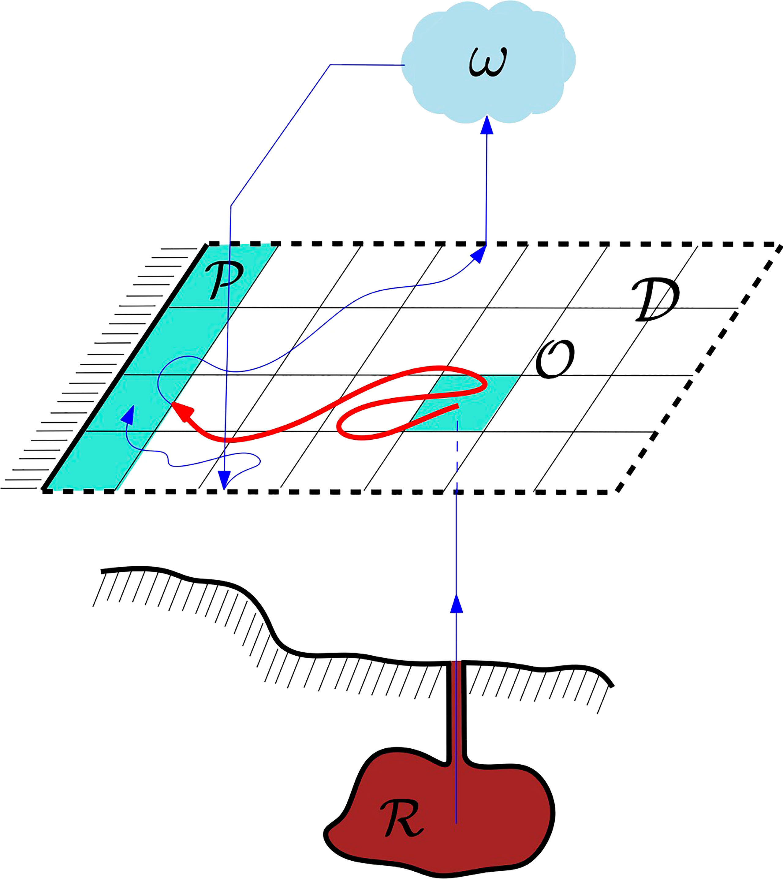
Figure 1 The framework for the TPT-based prediction scheme is an autonomous, discrete-time Markov chain on a state space given by the box covering of a two-dimensional, open ocean domain, 𝒟, augmented by two virtual boxes or states. One state, called a two-way nirvana state and denoted by ω , compensates for probability mass imbalances due to the openness of 𝒟. The other state, called an oil reservoir state and denoted by ℛ, injects probability mass into the chain through the spill site, 𝒪⊂𝒟. Highlighted in red is the restriction to 𝒟 of a reactive trajectory connecting ℛ with 𝒫 ⊂ 𝒟, a region that is targeted to be protected, chosen to be the shoreline in the cartoon. Such a trajectory flows last from ℛ and next goes to 𝒫, while being constrained to stay in 𝒟, once it enters 𝒟. So defined, a reactive trajectory of oil may return back many times to the spill site before reaching the protected area. TPT provides a statistical characterization of the ensemble of reactive trajectories, highlighting the dominant paths of oil into 𝒫. The reentry into 𝒟 from ω uses information available from trajectory data outside 𝒟. There are many reentry doors; we depict, for illustrative purposes, the trajectory through one such doors.

Inclusion of a two-way nirvana state is not new, as it was first applied by Miron et al. (2021) to treat transition paths of marine debris into the subtropical oceans’ great garbage patches. Additional TPT applications involving this type of closure include those detailed in Refs (Beron-Vera et al., 2022a; Beron-Vera et al., 2022b; Drouin et al., 2022; Miron et al., 2022). The use of an oil reservoir state is novel in TPT.

2.3 A proposal for using transition path theory to predict oil paths and arrival

We propose to apply TPT such that it makes use of available oil trajectories up to the present, to make a prediction beyond, so it does not rely on forecasted oil trajectories. This follows precedent work (Olascoaga and Haller, 2012), which was able to predict sudden changes in the shape of the oil slick during the Deepwater Horizon spill. The expectation is that such a type of prediction should be superior than that based on forecasted velocities, which are not validated by data as is the case of hindcast velocities from an analysis system. Moreover, when available, the scheme enables the use of velocities inferred from high-frequency radar measurements and even trajectories of appropriate satellite-tracked surface drifting buoys.

The proposed prediction scheme more specifically consists in applying TPT using trajectories over a few time steps prior to the prediction time, say t₀=n₀T . That is, we propose to compute the closed transition matrix $\tilde{P}$ for the augmented Markov chain on $\tilde{\mathcal{D}}$, as given by Eq. 14, and the various TPT statistics from it according to Proposition 1, by making use of all trajectories available over t∈{(n₀−m)T,…,(n₀−1)T,n₀T} for some m≤n₀ . This way, a prediction for the spilled oil distribution on t=(n₀+1)T , in direct transition into the region to be protected, P, is obtained. The skeleton thereof will be provided by the two-dimensional vector field taking values at discrete positions x_i , where x_i is the center of box B_i∈𝒟 , given by

$\begin{array}{ll}J(x_i):={\displaystyle \sum _{j\in \mathcal{D}}}{\tilde{f}}_{ij}^{+}e(i,j),& (18)\end{array}$

where e(i,j) is the (two-dimensional) unit vector pointing from x_i to x_j, the center of box B_j∈𝒟 . The above is a visualization means of reactive probability flux, proposed in (Helfmann et al., 2020). We will refer to Eq. 18 as the reactive current at position x_i . The prediction can be updated, as we will do in the examples we provide below, by computing TPT using trajectories within time windows sliding over the prediction time t₀ (or n₀).

In the present exploratory work, the oil evolution in every case will be obtained by pushing forward a probability vector on $\tilde{\mathcal{D}}$ with support in ℛ at time t=0 , namely,

$\begin{array}{ll}\tilde{o}(0)=\frac{{\tilde{1}}_{ℛ}}{\left|ℛ\right|},& (19)\end{array}$

under right multiplication by a nonautonomous version of the augmented chain transition matrix $\tilde{P}$ in Eq. 14. Denoted by $\tilde{P}(n)$ to make explicit its dependence on t=nT , this will be constructed by accounting for the start time t in the estimation of P in Eq. 13. To add a bit of extra realism, we will set p^ℛ→ℛ in Eq. 14 to

$\begin{array}{ll}{p}^{ℛ\to ℛ}(n)=\frac{1}{N-n+1},& (20)\end{array}$

representing an oil reservoir that is drying over the time interval t∈{0,T,2T,…,NT} . Indeed, when n=N , p^ℛ→ℛ=1 , meaning that the probability mass flux into the ocean domain 𝒟 through the oil spill site 𝒪 is nil. That is, the reservoir ℛ has completely dried out by t=NT. This assumption may be adapted based on any information available about how quickly the oil reservoir may be expected to empty or a spilling oil well may be capped. The total accumulated oil, which flows out from ℛ into D through O in an uninterruptedly but decaying in time manner, at discrete time t=nT will be given by $o(n)=\tilde{o}(n){|}_{\mathcal{D}}$ , where

$\begin{array}{ll}\tilde{o}(n)=\tilde{o}(0)\left(\text{Id }+{\displaystyle \sum _{k=0}^{n-1}}{\displaystyle \prod _{l=k}^{n-1}}\tilde{P}(l)\right).& (21)\end{array}$

Note that $\tilde{o}(n)$, and hence o(n), does not need to be a probability vector, and the units in which o(n) is measured are determined by the units assigned to $\tilde{o}(0)$.

To incorporate the effects of a drying oil reservoir in the TPT prediction step, the autonomous transition matrix $\tilde{P}$ used in that step will have to be constructed using p^ℛ→ℛ in Eq. 14 as the average value of over the corresponding time interval.

The idea of using trajectory information up to the present prevents us from using the extension of TPT for time-inhomogeneous Markov chains proposed in (Helfmann et al., 2020), as it might be thought to be more suitable for a prediction scheme in a naturally time-varying environment. The reason is that, as formulated, nonautonomous TPT requires unavailable trajectory information and knowledge of when P will be hit by transition paths.

A final comment is reserved to the oil trajectories themselves. If u(x,t) denotes the surface ocean velocity, as output from an ocean circulation model, and u₁₀(x,t) is the wind velocity at 10 m above the sea surface, as produced by some atmospheric circulation model, the oil trajectories will here be obtained by integrating

$\begin{array}{ll}\dot{x}=u(x,t)+\alpha u_{10}(x,t),0<\alpha \ll 1,& (22)\end{array}$

for many initial conditions over a domain including the ocean domain D of interest; thus, reentry information, namely, that required to evaluate p^O←ω in Eq. 14, is available. Equation 22 is a minimal law for oil parcel motion (Abascal et al., 2009; Abascal et al., 2012). It exclusively accounts for the wind action on oil parcels, neglecting weathering effects. Typically employed values of α range from 2% to 4% (ASCE, 1996).

3 Results

3.1 Hypothetical oil spill in the Trion field

We begin by applying our proposed TPT-based prediction scheme to a hypothetical oil spill in the Trion field, located within the Perdido Foldbelt, a geological formation in the northeastern Gulf of Mexico with an important oil reservoir for ultradeepwater drilling under development (Offshore Technology, 2020). This will be done by considering two different velocity representations.

In the first representation, u in Eq. 22 is chosen to be given by a daily climatology of surface velocity constructed from velocities over 18 years (1995–2012) produced by a free-running regional configuration for the Gulf of Mexico at 1/36^∘ horizontal resolution (Jouanno et al., 2016) of the ocean component of the Nucleus for European Modelling of the Ocean (NEMO) system (Madec and the NEMO team, 2016). This dataset was used in (Gough et al., 2019) to investigate persistent passive tracer transport patterns using so-called climatological Lagrangian coherent structures (cLCSs) (Duran et al., 2018). A main finding was the presence of a mesoscale hook-like cLCS providing a barrier for cross-shelf transport nearly year-round. Consistent with the motion of historical satellite-tracked drifting buoys, with the majority of them including a drogue, albeit shallow (cf (Miron et al., 2017) for details), synthetic drifters originating beyond the shelf were found to be initially attracted to this cLCS as they spread anticyclonically and eventually over the deep ocean. In (Gough et al., 2019), it is noted that this should have implications for the mitigation of contaminant accidents such as oil spills. This picture, however, may be altered for oil, as this is expected to be influenced by the wind action, which, in (Gough et al., 2019), was not accounted for when winds are strong. To evaluate their effect, we need a representation for u₁₀ in Eq. 22, which is chosen to be provided by daily climatological wind velocity at 10 m height from the European Centre for Medium-Range Weather Forecasts (ECMWF) atmospheric reanalysis ERA-Interim (Dee et al., 2011).

In Figure 2, we present our first set of results. These are based on the use of trajectories obtained by numerically integrating Eq. 22 with the daily climatological NEMO + ECMW velocity data above, using a fourth-order Runge–Kutta scheme with cubic interpolation in space and time. The integrations, reinitialized every day along the month of February, span T=1 day. We consider initial conditions distributed uniformly over an ocean domain larger (by 1^∘ to the east and south) than that one (𝒟) contained inside [98^∘ W, 93^∘ W] × [24 ^∘ N, 30 ^∘ N], shown in Figure 2. To evaluate the transition matrix on 𝒟, using Eq. 13, we cover 𝒟 with boxes of about 1/6^∘ side, including roughly 100 test points per box when trajectories initialized once are only considered. The transition time step T=1 day guarantees sufficient loss of memory into the past for the Markovian assumption to hold; indeed, the typical decorrelation timescale on ocean surface is not longer than 1 day as estimated from drogue drifting buoys (LaCasce, 2008) and is likely to be even shorter when the wind action is accounted for. Stationarity of the Markov chain on the extended domain $\tilde{\mathcal{D}}$ is checked numerically. That is, we check that the largest eigenvalue of the transition matrix $\tilde{P}$ has multiplicity 1, and is equal to 1, to numerical precision. However, in the computation of P, namely, the transition matrix on the open domain 𝒟, we make sure to allow as much communication as possible along the corresponding Markov chain by applying Tarjan’s (Tarjan, 1972) algorithm on the associated directed graph, as we have done in earlier work [e.g (Miron et al., 2017; Miron et al., 2019a; Miron et al., 2019b; Beron-Vera et al., 2020]. This can result in some boxes of the covering of the ocean domain to be excluded, particularly when dealing with observed (satellite-tracked) trajectories, as we consider in Section 3.2 below.

FIGURE 2

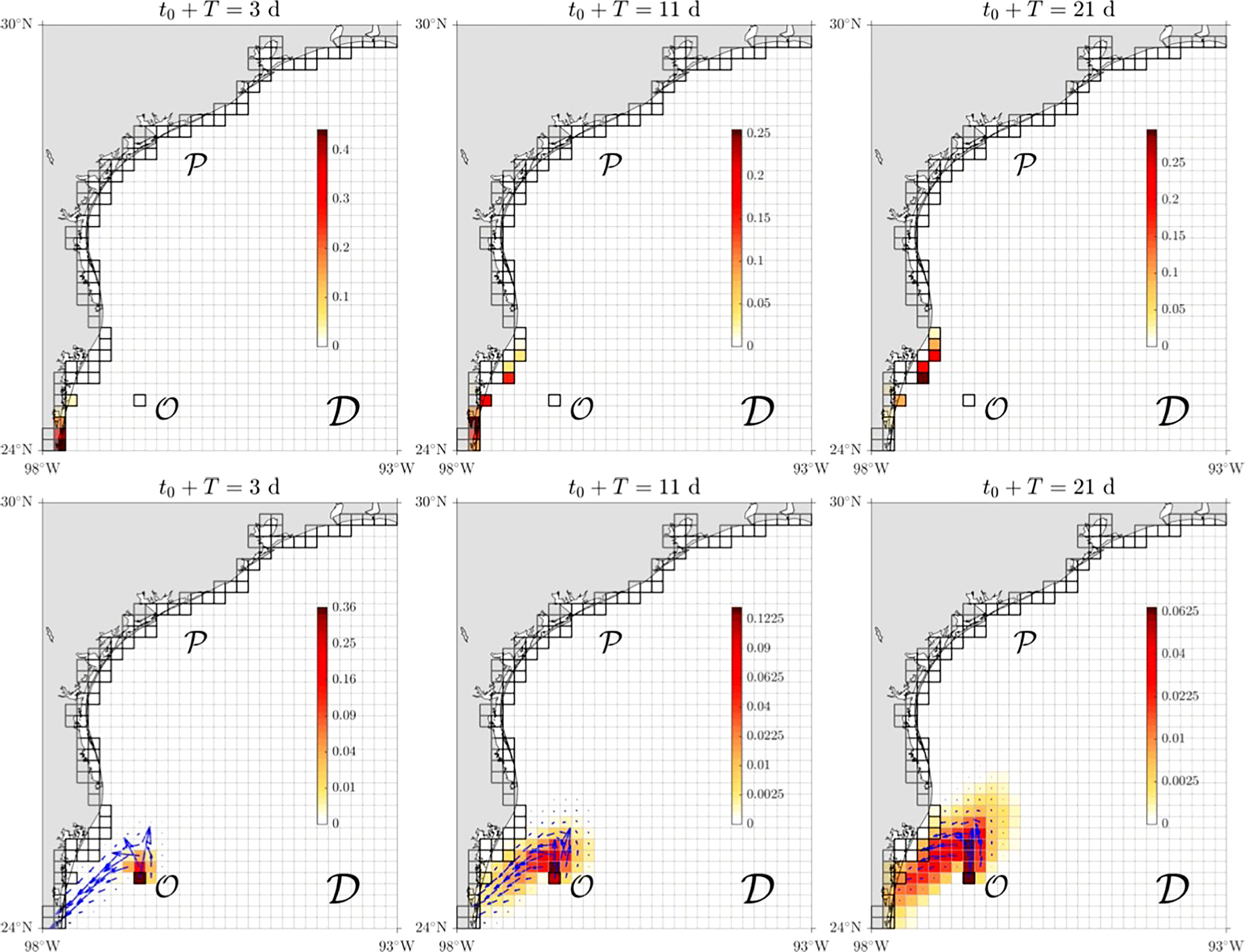
Figure 2 (Top panels) Based on the daily climatological NEMO + ECMW oil velocity model, predictions on time t=t₀ of (normalized) reactive rates of arrival of transition paths, through the open northwestern Gulf of Mexico domain 𝒟 and into the coastline (𝒫), of oil emerging from a hypothetical open well in the Trion field (𝒪), located within the Perdido Foldbelt, since t=0, corresponding to February 1. The transition time step, T=1 day. (Bottom panels) Relative distribution of accumulated oil on t=t₀+T, overlaid with predicted (on t=t₀ ) reactive currents, indicating transition oil paths into 𝒫.

With 𝒪, the oil spill site, taken to be a box of the covering of 𝒟 closest to the Trion field and 𝒫, the region to be protected, taken to be the coastal boxes, the top row of Figure 2 shows the predicted reactive rate of (oil) trajectories entering each box of 𝒫 for selected times since since 1 February when the oil spill is hypothetically initiated. Specifically, we show this normalized to a probability vector on 𝒟, viz.,

$\begin{array}{ll}\mathbf{k }:={\displaystyle \sum _{i\in P}\frac{{\tilde{k}}^{R{B}_i}}{{\displaystyle {\sum }_{i\in P}{\tilde{k}}^{R{B}_i}}}{{\mathbf{1}}_{B_i}|}_p,{\tilde{k}}^{R{B}_i}={\displaystyle \sum _{l\in D}{\tilde{f}}_{li}={\displaystyle \sum _{l\in D}{\tilde{f}}_{il},} i\in 𝒫,}}& (23)\end{array}$

where the TPT computation follows Proposition 1. More precisely, in the TPT calculation, we apply Proposition 1 for each i ∈ 𝒫, i.e., with P replaced by i ∈ 𝒫. The transition matrix of the augmented chain in $\tilde{\mathcal{D}}$, given by Eq. 14, is computed using trajectories over t∈{t₀−2T,t₀−T,t₀} for every t₀ in Figure 2. The coastal boxes that are predicted to be most affected by the oil spill correspond to those where components of k in Eq. 23 take the largest values. Note, in this case, that the predicted coastal boxes that will be most affected change over time, moving from the boxes corresponding to the Mexican state of Tamaulipas north toward the international border with the United States. This is consistent with the updated reactive current predictions and, most importantly, with the portion of the simulated spilled oil distribution directed into the coastline. This is depicted in the bottom row of Figure 2. More specifically, the heatmap in each panel is of $o(n_0+1)=\tilde{o}(n_0+1){|}_{\mathcal{D}}$, with $\tilde{o}(n)$ given in Eq. 21, but normalized to a probability vector, giving the relative distribution of oil that has accumulated on 𝒟 at time t=t₀+T=(n₀+1)T. Overlaid on each heatmap are the predicted reactive currents (Eq. 18) on each t₀. These are seen to anticipate, T=1 day in advance, the motion of the oil directed into the coastline quite well. An important observation is that the main factor responsible for this motion is the wind action on the oil, which makes it bypass the cross-shelf transport barrier for passive tracers shown (Gough et al., 2019) to be supported nearly year-round by the climatological NEMO surface ocean velocity field. Indeed, the winter season is dominated by “nortes” (Gómez Ramírez and Reséndiz Espinosa, 2002). These are strong, predominantly northerly winds suddenly produced after the passage of a cold front, which, imprinted in the daily climatology, promote the accumulation of the oil toward the coastline.

In addition to predicting the transition paths of oil into the coastline, TPT can give a prediction for the arrival time of the oil. Using the reaction duration formula (Eq. 12), but on the extended Markov chain on $\tilde{\mathcal{D}}$ and for each i ∈ 𝒫, as done to compute the reaction rate (Eq. 23), we compute on t₀=2 days, the first time a prediction can be made, that

$\begin{array}{ll}\underset{i\in P}{\min }\left\{{\tilde{t}}^{R{B}_i}\right\}=\underset{i\in P}{\min }\left\{\frac{{{\displaystyle {\sum }_{l\in \tilde{D}}\tilde{\pi }}}_l^{\mathcal{R}{B}_i}}{{\tilde{k}}^{R{B}_i}/T}\right\}\approx 14days.& (24)\end{array}$

early prediction turns out be somewhat longer than the actual arrival time to the coast, which happens approximately 11 days after the (simulated) oil started. This assessment is rough, based on when oil probability mass is found for the first time in a coastal box, independent of how much. With this in mind, early prediction (Eq. 24) is not that off at all, but one may wonder if it could be updated with time, i.e., as newer data become available. This is hopeless using Eq. 12, as it computes the duration of the whole reaction from source to target, which are fixed in space. However, the desired update of the arrival time prediction may indeed be accomplished. We discuss how in the last section.

The second representation for u in Eq. 22 that we consider is provided by hourly surface ocean velocity output from the HYCOM (HYbrid-Coordinate Ocean Model) + NCODA (Navy Coupled Ocean Data Assimilation) Gulf of Mexico 1/25^∘ Analysis (GOMu0.04/expt_90.1m000) (Chassignet et al., 2007). For u₁₀ in Eq. 22, we use three-hourly wind velocity, 10 m above the sea surface, from the National Centers for Environmental Prediction (NCEP) operational Global Forecast System (GFS) analysis and forecast at 1/4^∘ horizontal resolution (National Centers for Environmental Prediction et al., 2015). In neither case did we consider forecasted velocities; instead, we considered a record, from 22 July 2022 through 8 August 2022, of hindcast velocities, i.e., as produced by the systems while they assimilated observations “on the fly” to make the forecasts. The TPT setup for the HYCOM + NCEP oil velocity is similar to that for the climatological NEMO + ECMWF oil velocity. For instance, trajectory integrations are reinitialized daily and span T=1 day, and the number of boxes of the domain partition is similar to a comparable number of test points per box. Unlike the climatological case, the time origin (t=0 ) of the oil spill simulation corresponds to a specific day of the current year, chosen to be 22 July 2022. The simulation extends out to 8 August 2022. Covering a summer time period, it is not affected by “nortes” wind events, which prevail in winter. The results are shown in Figure 3. As can be expected, an important difference with those shown in Figure 2 is a stronger influence of the cross-shelf transport barrier for passive tracers on the distribution of the simulated oil, which, while eventually reaching the coastline, starts to develop a hook-like shape pointing into the open ocean by t=16 days, similar to that described in (Gough et al., 2019). This happens after part of the oil is trapped in an anticyclonic circulation. The predicted arrival location on t₀=2 days falls quite close to the arrival location, which takes place between the southern Texas cities of Corpus Christi and Galveston on t≈9 days. The early prediction (on t₀=2 days) of arrival time is t≈6 days, which is shorter than the arrival time, calling for an update.

FIGURE 3

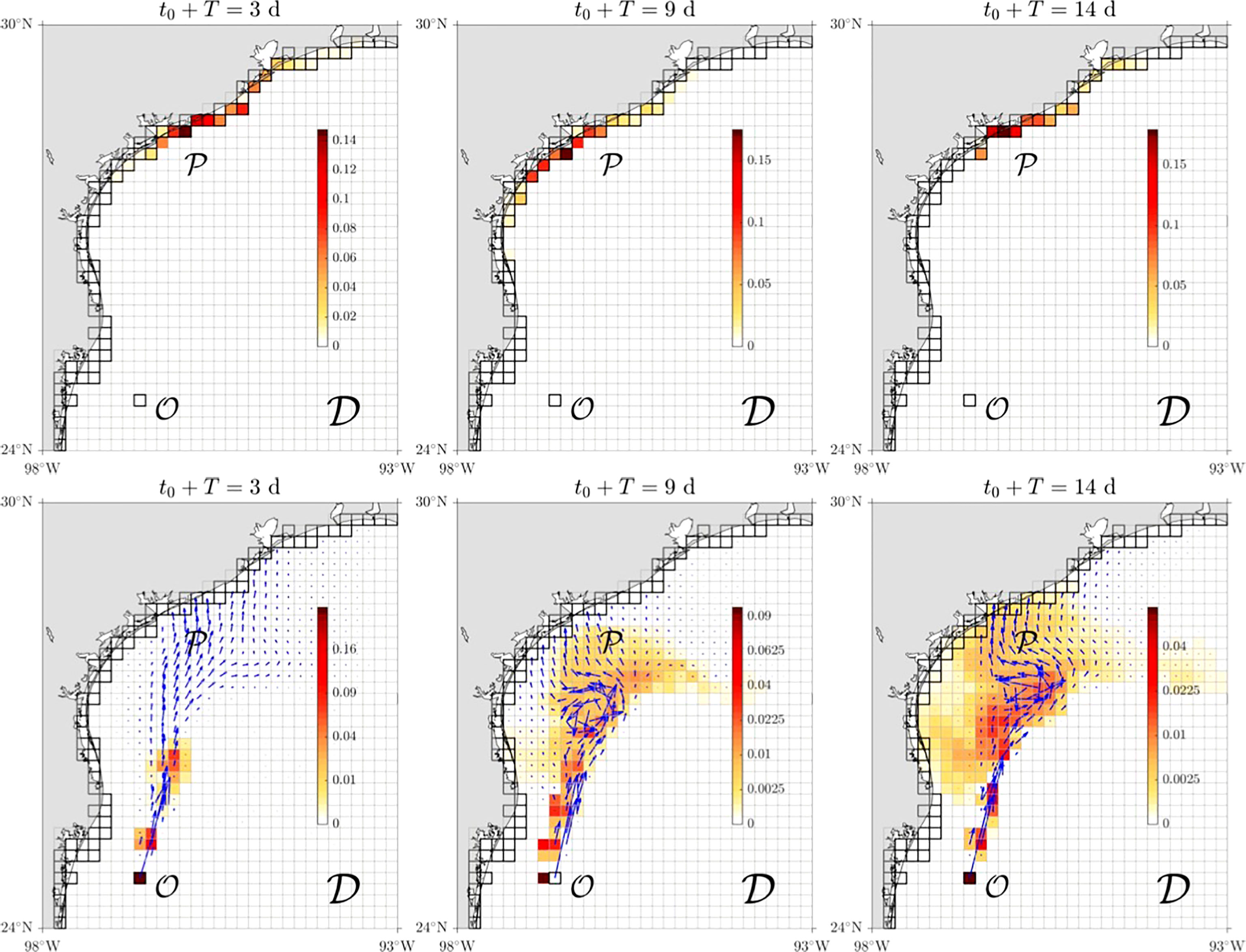
Figure 3 As in Figure 2, but based on the HYCOM + NCEP oil velocity model and t=0 corresponding to 22 July 2022.

Overall, the above results provide support to our proposed TPT-based oil spill prediction scheme, based on the assumption that the motion prior to the prediction time is representative of motion beyond it, for some time, which we test against observations in the section that follows.

3.2 The Deepwater Horizon oil spill

The basic assumption on which the TPT-based oil prediction scheme builds on, namely, that environmental conditions prior to the prediction time can be prolonged beyond it, for some time, is here tested using oil arrival time estimates for the Deepwater Horizon spill (Crone and Tolstoy, 2010). Shown in the heatmap in the center panel of Figure 4, the arrival time estimates are inferred using available satellite images of the oil slick, as produced by the National Oceanic and Atmospheric Administration (NOAA) National Environmental Satellite Data and Information Service (NESDIS) Marine Pollution Surveillance Program (Streett, 2011). The time origin is 22 April 2010, when the Macondo well started to spill oil due to the sinking of the mobile offshore rig after an explosion caused by a blowout 2 days before (Crone and Tolstoy, 2010). The value assigned to each colored pixel corresponds to the first time (in days) the oil visited that pixel.

FIGURE 4

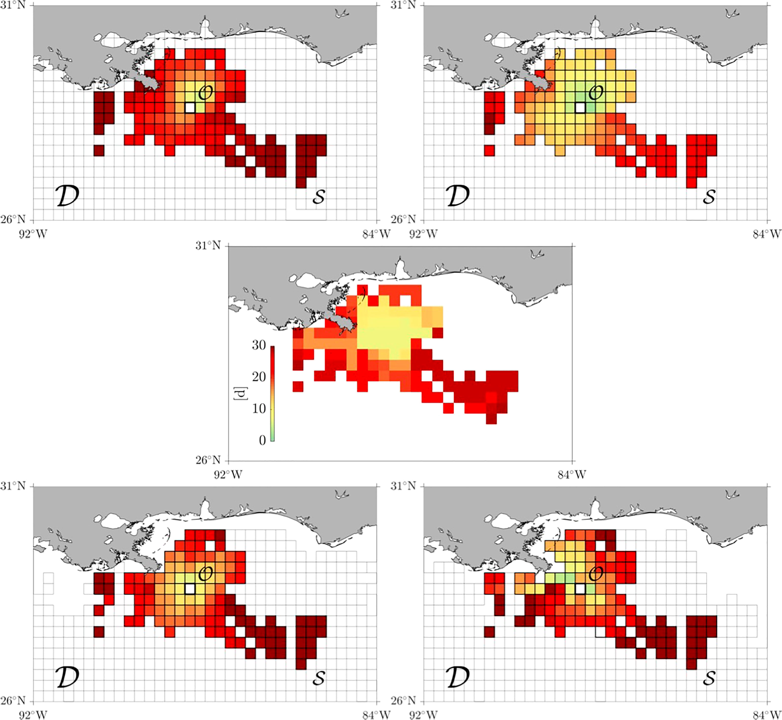
Figure 4 Estimated from satellite images of the Deepwater Horizon oil slick, time to first find oil on the surface of the ocean since 22 April 2010, when the spill started to spill from the Macondo well (center panel), along with the reaction duration of transition paths into each box of the subset 𝒮 of the domain covering 𝒟 that most closely intersects the region visited by the surfaced oil according to trajectories integrated from surface NCOM velocities (top left panel) and the latter with the addition of 3% NOAA/NCEI windage (top right panel) over a period of 7 days prior to the first time oil was found on the ocean surface on 29 April 2010, and trajectories produced by historical satellite-tracked surface drifters with drogue present (bottom left panel) and absent (bottom right panel).

Four TPT-based estimates, based on four different Markov chains, of the arrival time are shown in Figure 4, two in the top panels and two in bottom panels. More specifically, these are reaction durations (Eq. 12) into each box (B_i) of the set S of the domain covering (𝒟) that most closely intersects the region in the center panel of Figure 4 where the oil was observed to be occupied in the satellite imagery. More specifically, we show

$\begin{array}{ll}t:={{\displaystyle \sum _{i\in \mathcal{S}}}{\tilde{t}}^{ℛB_i}{\mathbf{1}}_{B_i}|}_{\mathcal{S}},& (25)\end{array}$

computed using Proposition 1 with P replaced by i∈S. The Markov chains are constructed as follows.

For the top panels of Figure 4, we use T= 1 -day-long trajectories integrated from Eq. 22 in the interval 22 April 2010 through 29 April 2010, the day when the satellite images record reveal oil on the surface for the first time (since the spill started, on 22 April 2010). For both panels, we use u in Eq. 22 represented by daily surface ocean velocities produced by the experimental real-time Intra-Americas Sea Nowcast/Forecast System (IASNF) at 1/25^∘ horizontal resolution, which is based on the U.S. Naval Coast Ocean Model (NCOM) (Ko et al., 2003). In turn, the wind (u₁₀) velocity representation is obtained from daily 1/4^∘ horizontal resolution winds at 10 m from the NOAA/National Centers for Environmental Information (NCEI) Blended Sea Winds product (Zhang et al., 2006). The difference between the top left and right panels is that in the former, the oil model velocity uses α=0 , i.e., the wind effect is shut off, and in the latter, α=0.03, as we have set above. The size of each box of the covering is 1/25^∘×1/25^∘, and the number of test points per box is (roughly) 100.

For the bottom panels of Figure 4, we consider pieces of length T=1 day of historical, i.e., available since 1992 to date, satellite-tracked trajectories of surface drifting buoys from the NOAA Global Drifter Program (GDP) (Lumpkin and Pazos, 2007) with the following distinction: in the left panel, we consider drifters that have their (15-m-long) drogues (sea anchors) attached at all times, while in the right panel, only those that do not have a drogue attached during the extent of the record (because this has been lost at the beginning of the record, after deployment, as assessed by the drogue presence algorithm of (Lumpkin et al., 2012), or because the drifter was intentionally deployed undrogued). The size of each box of the covering is. for the drogued and the undrogued drifters. The number of test points per box is small compared to that of the simulated oil trajectories, with only about test points per box.

Comparison of the top right panel of Figure 4 with the center panel reveals that our assumption that simulated trajectories up to the prediction time can be used to indeed make reliable predictions (beyond) holds quite well, at least for environmental conditions prevalent during the Deepwater Horizon spill, and during the timespan covered by the satellite imagery of the oil slick. In this case, windage in the minimal oil parcel trajectory model (Eq. 22) does not dramatically impact the TPT-based computation, as can be seen from the comparison of the top right panel with the top left panel. Recall that these use trajectories integrated over 7 days prior to the first time oil is observed on the ocean surface and that the satellite oil images record extends for 30 days. Moreover, even TPT results based on historical drifter trajectories are reasonable, irrespective of whether the drifters are drogued or undrogued, as it follows from the inspection of the bottom panels of Figure 4. These results might not come as a big surprise, as an analysis of daily climatological model velocities was successful in reproducing the “tiger tail” shape produced by the Deepwater Horizon oil slick (Duran et al., 2018). Similarly, the analysis of altimetry-derived surface ocean velocities was capable of reproducing a similar shape into which drifting buoys from the Grand Lagrangian Deployment (GLAD) organized along (Olascoaga et al., 2013).

Clearly, the above results for the Deepwater Horizon oil spill, the largest and best documented oil spill, may not be made extensible to other oil spills in other regions of the ocean and in seasons with more variable environmental conditions. Yet, they are an encouraging sign of the validity of the assumption on which our TPT-based oil prediction scheme builds on. In such more variable environments, a more sophisticated model than Eq. 22 may be needed and there is also ample space to improving the TPT setup. We highlight possible or required improvements below.

4 Summary and concluding remarks

In this paper, we have given the first steps toward building an oil spill prediction scheme based on the use of TPT for autonomous, discrete-time Markov chains on boxes, which cover a typically open flow domain, a result under an appropriate discretization of the oil motion, assumed to be described by a stationary stochastic process, namely, to obey an advection–diffusion with a steady velocity. Transition paths highlight the main conduits of communication between a source and a target in the phase of a dynamical system under noise, and thus, they can be used to unveil the main routes of oil from an accidental spill in the ocean into a region that needs protection.

The basic premise of the TPT-based oil prediction scheme is that trajectory information up to the prediction time can be used to infer oil motion beyond it. The TPT setup deviates from the standard TPT setup in that one needs to cope with the openness of ocean flow domain where a spill takes place, which is accounted for by the addition of a virtual box (state) that compensates for probability mass imbalances, and also with a way to represent the injection of oil in to the open flow domain, which is done via the addition of another virtual state representing an oil reservoir. The scheme was tested by considering a hypothetical oil spill in the Trion field, located within the Perdido Foldbelt in the northwestern Gulf of Mexico, and the Deepwater Horizon oil spill, giving good signs of its validity.

Several improvements to the proposed scheme are possible or required. These should help increase the quality of the predictions, particularly under environmental conditions that are more variable than those of the situations considered here.

• In the examples considered, the prediction time increment, say Δt₀ , was chosen to be equal to the transition time step (T). For the Markovianity assumption to be fulfilled, T should not be taken shorter than 1 day, the typical Lagrangian decorrelation time in the surface ocean. However, there is no restriction on the choice of Δt₀ , and the frequency of prediction updates may be higher than daily.

• In a similar manner to the prediction of transition paths of oil into the region one desires to protect being updated over time, the duration of the paths should also be updated, as it is not just where oil will end that needs to be known, but when it will arrive at the protected area. This will require one to compute the reaction duration into the target region from any place in between it and the source. Mathematically, this is given by the expectation of the random time to first enter the target conditioned on starting on any box (state) of the chain while the trajectory is reactive. A collection of such boxes can be chosen to be those where the updated reaction distribution (Eq. 9), which tells one where the reactive flux bottlenecks are, acquires the largest values. There is currently no TPT formula that accounts for this in the case of the Markov chain setting of this paper. For diffusion processes, a related statistic is derived in (Finkel et al., 2021).

• Another aspect that we have not accounted for is oil beaching. This is an additional source of openness of the flow domain. Beaching has been incorporated in a physically consistent manner in the problem of plastic pollution (Miron et al., 2021). Such a solution does not seem appropriate for the oil problem, and beaching may necessarily result in a nonstationary Markov chain. The nonautonomous extension of TPT in (Helfmann et al., 2020) does not require the Markov chain to be stationary, which may provide a resolution to this aspect. However, nonautonomous TPT requires trajectory information past the prediction time, and thus, a different strategy to cope with beaching will need to be designed.

• Last but not least is the oil parcel trajectory model. We have considered the minimal possible model, which only accounts for windage in a bulk manner. The typically used windage accounts for the effects of wave-induced Stokes drift, which may be explicitly added to the ocean surface velocity with the corresponding reduction of the windage. The Stokes drift may be obtained from a wave model. The full ocean surface plus wave-induced drift is measured, partially at least (Graber et al., 1997; Röhrs et al., 2015), by high-frequency radars, which, when available, may be easily incorporated. Additional improvements may be provided by the Maxey–Riley theory for floating material on the ocean surface (Beron-Vera et al., 2019; Olascoaga et al., 2020), which includes a law for windage depending on buoyancy in closed form, or consideration of the output from an oil spill trajectory model like OpenDrift, which accounts for weathering effects, as noted in the Introduction. The trajectories produced by the minimal model or improvements thereof may be combined with trajectories of satellite-tracked appropriate drifting buoys, if these are deployed in the area where the oil spill takes place.

Data availability statement

The ECMWF/ERA Interim wind renanalysis can be obtained from https://apps.ecmwf.int/datasets/data/interim-full-daily/levtype=sfc/. The Gulf of Mexico HYCOM+NCODA analysis data are available at https://www.hycom.org/data/gomu0pt04/expt-90pt1m000. The NCEP/GFS wind data can be retrieved from https://www.ncei.noaa.gov/products/weather-climate-models/global-forecast. Digitized versions of the observed surface ocean oil distribution images during the Deepwater Horizon spill are available at https://satepsanone.nesdis.noaa.gov/pub/OMS/disasters/DeepwaterHorizon/composites/2010/. The NCOM/IASNFS output is available from https://www.northerngulfinstitute.org/edac/oceanNomads/IASNFS.php. The NOAA/NEIC wind data are available from https://coastwatch.pfeg.noaa.gov/erddap/griddap/ncdcOwClm9505.html. The NOAA/GDP drifter data are available at https://www.aoml.noaa.gov/phod/gdp/.

Author contributions

All authors listed have made a substantial, direct, and intellectual contribution to the work and approved it for publication.

Funding

Support for this work was provided by Consejo Nacional de Ciencia y Tecnología (CONACyT)–Secretaría de Energía (SENER) as part of the Consorcio de Investigación del Golfo de México (CIGoM).

Acknowledgments

We thank Luzie Helfmann and Péter Koltai for discussions on adapting TPT to the oil spill problem, and Joaquin Triñanes for making the Deepwater Horizon oil spill imagery available to us.

Conflict of interest

The authors declare that the research was conducted in the absence of any commercial or financial relationships that could be construed as a potential conflict of interest.

Publisher’s note

All claims expressed in this article are solely those of the authors and do not necessarily represent those of their affiliated organizations, or those of the publisher, the editors and the reviewers. Any product that may be evaluated in this article, or claim that may be made by its manufacturer, is not guaranteed or endorsed by the publisher.

References

Abascal A. J., Castanedo S., Fernández V., Medina R. (2012). Backtracking drifting objects using surface currents from high-frequency (HF) radar technology. Ocean Dynamics 62, 1073–1089. doi: 10.1007/s10236-012-0546-4

CrossRef Full Text | Google Scholar

Abascal A. J., Castanedo S., Medina R., Losada I. J., Alvarez-Fanjul E. (2009). Application of HF radar currents to oil spill modelling. Mar. pollut. Bull. 58, 238–248. doi: 10.1016/j.marpolbul.2008.09.020

PubMed Abstract | CrossRef Full Text | Google Scholar

ASCE (1996). State-of-the-art review of modeling transport and fate of oil spills. J. Hydraulic Engr. 122, 594–609. doi: 10.1061/(ASCE)0733-9429(1996)122:11(594)

CrossRef Full Text | Google Scholar

Beegle-Krause J. (2001). General NOAA oil modeling environment (GNOME): A new spill trajectory model. Int. Oil Spill Conf. Proc. 2001, 865–871. doi: 10.7901/2169-3358-2001-2-865

CrossRef Full Text | Google Scholar

Beron-Vera F. J., Bodnariuk N., Saraceno M., Olascoaga M. J., Simionato C. (2020). Stability of the malvinas current. Chaos 30, 013152. doi: 10.1063/1.5129441

PubMed Abstract | CrossRef Full Text | Google Scholar

Beron-Vera F. J., Olascoaga M. J., Helfmann L., Miron P. (2022b). Sampling-dependent transition paths of Iceland–Scotland overflow water. J. Phys. Oceanogr. doi: 10.1175/JPO-D-22-0172.1

CrossRef Full Text | Google Scholar

Beron-Vera F. J., Olascoaga M. J., Miron P. (2019). Building a maxey–Riley framework for surface ocean inertial particle dynamics. Phys. Fluids 31, 096602. doi: 10.1063/1.5110731

CrossRef Full Text | Google Scholar

Beron-Vera F. J., Olascoaga M. J., Putman N. F., Trinanes J., Lumpkin R., Goni G. (2022a). Dynamical geography and transition paths of sargassum in the tropical Atlantic. AIP Adv., 105107. doi: 10.21203/rs.3.rs-1594768/v1

CrossRef Full Text | Google Scholar

Chassignet E. P., Hurlburt H. E., Smedstad O. M., Halliwell G. R., Hogan P. J., Wallcraft A. J., et al. (2007). The HYCOM (HYbrid coordinate ocean model) data assimilative system. J. Mar. Sys. 65, 60–83. doi: 10.1016/j.jmarsys.2005.09.016

CrossRef Full Text | Google Scholar

Coelho E. F., Hogan P., Jacobs G., Thoppil P., Huntley H., Haus B., et al. (2015). Ocean current estimation using a multi-model ensemble kalman filter during the grand Lagrangian deployment experiment (GLAD). Ocean Modell 87, 86–106. doi: 10.1016/j.ocemod.2014.11.001

CrossRef Full Text | Google Scholar

Crone T. J., Tolstoy M. (2010). Magnitude of the 2010 gulf of Mexico oil leak. Science, 634. doi: 10.1126/science.1195840

CrossRef Full Text | Google Scholar

Dagestad K. F., Rohrs J., Breivik O., Adlandsvik B. (2018). OpenDrift v1.0: a generic framework for trajectory modelling. Geoscientific Model. Dev. 11, 1405–1420. doi: 10.5194/gmd-11-1405-2018

CrossRef Full Text | Google Scholar

Dee D. P., Uppala S. M., Simmons A. J., Berrisford P., Poli P., Kobayashi S., et al. (2011). The ERA-interim reanalysis: configuration and performance of the data assimilation system. Quart. J. R. Met. Soc 137, 553–597. doi: 10.1002/qj.828

CrossRef Full Text | Google Scholar

Drivdal M., Broström G., Christensen K. H. (2014). Wave-induced mixing and transport of buoyant particles: application to the statfjord a oil spill. Ocean Sci. 10, 977–991. doi: 10.5194/os-10-977-2014

CrossRef Full Text | Google Scholar

Drouin K. L., Lozier M. S., Beron-Vera F. J., Miron P., Olascoaga M. J. (2022). Surface pathways connecting the south and north Atlantic oceans. Geophysical Res. Lett. 49, e2021GL096646. doi: 10.1029/2021GL096646

CrossRef Full Text | Google Scholar

Duran R., Beron-Vera F. J., Olascoaga M. J. (2018). Extracting quasi-steady Lagrangian transport patterns from the ocean circulation: An application to the gulf of Mexico. Sci. Rep. 8, 5218. doi: 10.1038/s41598-018-23121-y

PubMed Abstract | CrossRef Full Text | Google Scholar

E W., Vanden-Eijnden E. (2006). Towards a theory of transition paths. J. Stat. Phys. 123, 503–623. doi: 10.1007/s10955-005-9003-9

CrossRef Full Text | Google Scholar

Finkel J., Abbot D. S., Weare J. (2020). Path properties of atmospheric transitions: Illustration with a low-order sudden stratospheric warming model. J. Atmospheric Sci. 77, 2327–2347. doi: 10.1175/JAS-D-19-0278.1

CrossRef Full Text | Google Scholar

Finkel J., Webber R. J., Gerber E. P., Abbot D. S., Weare J. (2021). Learning forecasts of rare stratospheric transitions from short simulations. Monthly Weather Rev. 149, 3647–3669. doi: 10.1175/MWR-D-21-0024.1

CrossRef Full Text | Google Scholar

Gómez Ramírez M., Reséndiz Espinosa I. N. (2002). Seguimiento de nortes en el litoral del golfo de méxico en la temporada 1999–2000. Rev. Geográfica 131, 5–19. doi: 10.2307/40992822

CrossRef Full Text | Google Scholar

Gough M. K., Beron-Vera F. J., Olascoaga M. J., Sheinbaum J., Juoanno J., Duran R. (2019). Persistent transport pathways in the northwestern gulf of Mexico. J. Phys. Oceanogr. 49, 353–367. doi: 10.1175/JPO-D-17-0207.1

CrossRef Full Text | Google Scholar

Graber H. C., Haus B. K., Chapman R. D., Shay L. K. (1997). HF radar comparisons with moored estimates of current speed and direction: Expected differences and implications. J. Geophysical Research: Oceans 102, 18749–18766. doi: 10.1029/97JC01190

CrossRef Full Text | Google Scholar

Helfmann L., Borrell E. R., Schütte C., Koltai P. (2020). Extending transition path theory: Periodically driven and finite-time dynamics. J. Nonlinear Sci. 30, 3321–3366. doi: 10.1007/s00332-020-09652-7

CrossRef Full Text | Google Scholar

Jouanno J., Ochoa J., Pallas-Sanz E., Sheinbaum J., Andrade-Canto F., Candela J., et al. (2016). Loop current frontal eddies: Formation along the campeche bank and impact of coastally trapped waves. J. Phys. Oceanogr. 46, 3339–3363. doi: 10.1175/JPO-D-16-0052.1

CrossRef Full Text | Google Scholar

Ko D. S., Preller R. H., Martin P. J. (2003). An experimental real-time intra-americas Sea ocean Nowcast/Forecast system for coastal prediction. Proc. AMS 5th Conf. Coast. Atmospheric Oceanic Prediction Processes, 97–100.

Google Scholar

Koltai P. (2010). Efficient approximation methods for the global long-term behavior of dynamical systems – theory, algorithms and examples. Ph.D. thesis, Technical University of Munich, Munich.

Google Scholar

Kovács Z., Tél T. (1989). Scaling in multifractals: Discretization of an eigenvalue problem. Phys. Rev. A 40, 4641–4646. doi: 10.1103/PhysRevA.40.4641

CrossRef Full Text | Google Scholar

LaCasce J. H. (2008). Statistics from Lagrangian observations. Progr. Oceanogr. 77, 1–29. doi: 10.1016/j.pocean.2008.02.002

CrossRef Full Text | Google Scholar

Liu Y., Hickey D. P., Minteer S. D., Dickson A., Calabrese Barton S. (2019). Markov-State transition path analysis of electrostatic channeling. J. Phys. Chem. C 123, 15284–15292. doi: 10.1021/acs.jpcc.9b02844

CrossRef Full Text | Google Scholar

Lumpkin R., Grodsky S. A., Centurioni L., Rio M. H., Carton J. A., Lee D. (2012). Removing spurious low-frequency variability in drifter velocities. J. Atm. Oce. Tech. 30, 353–360. doi: 10.1175/JTECH-D-12-00139.1

CrossRef Full Text | Google Scholar

Lumpkin R., Pazos M. (2007). “Measuring surface currents with surface velocity program drifters: the instrument, its data and some recent results,” in Lagrangian Analysis and prediction of coastal and ocean dynamics. Eds. Griffa A., Kirwan A. D., Mariano A., Özgökmen T., Rossby T. (Cambridge University Press), 39–67.

Google Scholar

Madec G., the NEMO team (2016). NEMO ocean engine Vol. 27 (Note du Pole de modelisation de l’Institut Pierre-Simon Laplace), 386. Available at: https://www.nemo-ocean.eu/wp-content/uploads/NEMO_book.pdf.

Google Scholar

Meng Y., Shukla D., Pande V. S., Roux B. (2016). Transition path theory analysis of c-src kinase activation. Proc. Natl. Acad. Sci. 113, 9193–9198. doi: 10.1073/pnas.1602790113

CrossRef Full Text | Google Scholar

Metzner P., Schütte C., Vanden-Eijnden E. (2009). Transition path theory for Markov jump processes. Multiscale Modeling Simulation 7, 1192–1219. doi: 10.1137/070699500

CrossRef Full Text | Google Scholar

Miron P., Beron-Vera F. J., Helfmann L., Koltai P. (2021). Transition paths of marine debris and the stability of the garbage patches. Chaos, 033101. doi: 10.1063/5.0030535

PubMed Abstract | CrossRef Full Text | Google Scholar

Miron P., Beron-Vera F. J., Olascoaga M. J. (2022). Transition paths of north Atlantic deep water. J. Atmos. Oce. Tech. 39, 959–971. doi: 10.1175/JTECH-D-22-0022.1

CrossRef Full Text | Google Scholar

Miron P., Beron-Vera F. J., Olascoaga M. J., Froyland G., Pérez-Brunius P., Sheinbaum J. (2019b). Lagrangian Geography of the deep Gulf of Mexico. J. Phys. Oceanogr. 49, 269–290. doi: 10.1175/JPO-D-18-0073.1

CrossRef Full Text | Google Scholar

Miron P., Beron-Vera F. J., Olascoaga M. J., Koltai P. (2019a). Markov-Chain-inspired search for MH370. Chaos: Interdiscip. J. Nonlinear Sci. 29, 041105. doi: 10.1063/1.5092132

CrossRef Full Text | Google Scholar

Miron P., Beron-Vera F. J., Olascoaga M. J., Sheinbaum J., Pérez-Brunius P., Froyland G. (2017). Lagrangian Dynamical geography of the gulf of Mexico. Sci. Rep. 7, 7021. doi: 10.1038/s41598-017-07177-w

PubMed Abstract | CrossRef Full Text | Google Scholar

National Centers for Environmental Prediction, National Weather Service, NOAA, US Department of Commerce (2015). NCEP GFS 0.25 degree global forecast grids historical archive. doi: 10.5065/D65D8PWK

CrossRef Full Text | Google Scholar

Noé F., Schütte C., Vanden-Eijnden E., Reich L., Weikl T. R. (2009). Constructing the equilibrium ensemble of folding pathways from short off-equilibrium simulations. Proc. Natl. Acad. Sci. 106, 19011–19016. doi: 10.1073/pnas.0905466106

CrossRef Full Text | Google Scholar

Norris J. (1998). Markov Chains (Cambridge University Press).

Google Scholar

Offshore Technology (2020) Trion field, gulf of Mexico. Available at: https://www.offshore-technology.com/projects/trion-oil-field-gulf-of-mexico/.

Google Scholar

Olascoaga M. J., Beron-Vera F. J., Haller G., Trinanes J., Iskandarani M., Coelho E. F., et al. (2013). Drifter motion in the gulf of Mexico constrained by altimetric Lagrangian coherent structures. Geophys. Res. Lett. 40, 6171–6175. doi: 10.1002/2013GL058624

CrossRef Full Text | Google Scholar

Olascoaga M. J., Beron-Vera F. J., Miron P., Triñanes J., Putman N. F., Lumpkin R., et al. (2020). Observation and quantification of inertial effects on the drift of floating objects at the ocean surface. Phys. Fluids 32, 026601. doi: 10.1063/1.5139045

CrossRef Full Text | Google Scholar

Olascoaga M. J., Haller G. (2012). Forecasting sudden changes in environmental pollution patterns. Proc. Nat. Acad. Sci. U.S.A. 109, 4738–4743. doi: 10.1073/pnas.1118574109

CrossRef Full Text | Google Scholar

Pérez Brunius P., Turrent Thompson C., García Carrillo P. (2021). Escenarios oceánicos y atmosféricos de un derrame de petróleo en aguas profundas del golfo de méxico (Zenodo). doi: 10.5281/zenodo.5745572

CrossRef Full Text | Google Scholar

Röhrs J., Dagestad K. F., Asbjornsen H., Nordam T., Skancke J., Jones C. E., et al. (2018). The effect of vertical mixing on the horizontal drift of oil spills. Ocean Sci. 65, 1581–1601. doi: 10.5194/os-14-1581-2018

CrossRef Full Text | Google Scholar

Röhrs J., Sperrevik A. K., Christensen K. H., Broström G., Breivik O. (2015). Comparison of HF radar measurements with eulerian and Lagrangian surface currents. Ocean Dyn, 65, 679–690. doi: 10.1007/s10236-015-0828-8

CrossRef Full Text | Google Scholar

Romo-Curiel A., Ramirez-Mendoza Z., Fajardo-Yamamoto A., Ramírez-Leon M., García-Aguilar M., Herzka S., et al. (2022). Assessing the exposure risk of large pelagic fish to oil spills scenarios in the deep waters of the gulf of mexico. Mar. pollut. Bull. 176, 113434. doi: 10.1016/j.marpolbul.2022.113434

PubMed Abstract | CrossRef Full Text | Google Scholar

Shay L. K., Martinez-Pedraja J., Cook T. M., Haus B. K., Weisberg R. H. (2006). Surface current mapping using wellen radars. J. Atmos. Oceanogr. Tech 24, 484–503. doi: 10.1175/JTECH1985.1

CrossRef Full Text | Google Scholar

Spaulding M. L. (2017). State of the art review and future directions in oil spill modeling. Mar. pollut. Bull. 115, 7–19. doi: 10.1016/j.marpolbul.2017.01.001

PubMed Abstract | CrossRef Full Text | Google Scholar

Strahan J., Antoszewski A., Lorpaiboon C., Vani B. P., Weare J., Dinner A. R. (2021). Long- time-scale predictions from short-trajectory data: A benchmark analysis of the trp-cage miniprotein. J. Chem. Theory Comput. 17, 2948–2963. doi: 10.1021/acs.jctc.0c00933

PubMed Abstract | CrossRef Full Text | Google Scholar

Streett D. (2011). NOAA’s satellite monitoring of marine oil. Geophysical Monograph Ser 195, 9–18. doi: 10.1029/2011GM001104

Google Scholar

Tarjan R. (1972). Depth-first search and linear graph algorithms. SIAM J. Comput., 146–160. doi: 10.1137/0201010

CrossRef Full Text | Google Scholar

Thiede E. H., Giannakis D., Dinner A. R., Weare J. (2019). Galerkin approximation of dynamical quantities using trajectory data. J. Chem. Phys. 150, 244111. doi: 10.1063/1.5063730

PubMed Abstract | CrossRef Full Text | Google Scholar

W E., Vanden-Eijnden E. (2010). Transition-path theory and path-finding algorithms for the study of rare events. Annu. Rev. Phys. Chem. 61, 391–420. doi: 10.1146/annurev.physchem.040808.090412

PubMed Abstract | CrossRef Full Text | Google Scholar

Zhang H. M., Bates J. J., Reynolds R. W. (2006). Assessment of composite global sampling: Sea surface wind speed. Geophysical Res. Lett. 33, L17714. doi: 10.1029/2006GL027086

CrossRef Full Text | Google Scholar