AirSeaFluxCode: Open-source software for calculating turbulent air-sea fluxes from meteorological parameters

1 Introduction

1.1 Background & requirements

Surface heat and momentum fluxes play an important role in the Earth’s climate system, as they can affect large-scale circulation patterns in the atmosphere which in turn affect surface wind patterns which drive the general ocean circulation (Cronin et al., 2019). The quantification of heat (sensible and latent) and momentum fluxes in most applications relies on empirical parameterizations, often called bulk formulae, that relate the fluxes to relatively easily obtained mean variables such as near-surface wind speed, air and sea temperatures and humidity. These mean (or bulk) variables can be obtained from in situ measurements (Berry and Kent, 2009), satellite observations (e.g. Bentamy et al., 2017) or from reanalysis model output fields (e.g. Bosilovich et al., 2011; Dee et al., 2011; Kobayashi et al., 2015; Hersbach et al., 2020). The parameterizations take one of two equivalent forms to represent the complexities of air-sea exchange, either using transfer coefficients or by defining surface roughness lengths. The parameterizations themselves usually derive estimates of these coefficients or roughness lengths from direct measurements of the fluxes (using, e.g. the eddy covariance method which requires very precise, fast response instruments) made concurrently with measurements of the mean or bulk variables. Direct measurements of the turbulent fluxes can be highly uncertain even when made with extreme care (Bradley and Fairall, 2006), and are expensive and difficult to make so are therefore very sparse. The uncertainty inherent in direct turbulent flux measurements (Bradley and Fairall, 2006), and the limited extent to which they sample the range of important regimes (Yu, 2019), places a limit on the accuracy of the bulk parameterizations derived using those measurements (Taylor, 2000). As a result, there are large differences in the magnitude of the estimated turbulent surface fluxes (TSF) derived from different bulk formulae, particularly under high wind speeds when direct flux measurements are difficult to obtain, or very low wind speeds or in stable conditions when the underlying theory may not be applicable.

A commonly-cited requirement for climate applications is for global or basin-scale surface net fluxes on monthly to seasonal time scales to be better than 10 Wm⁻² for the heat fluxes and 0.01 Nm⁻² for the momentum flux (Taylor, 2000; Bradley and Fairall, 2006; Yu, 2019). Requirements for other applications are summarized by Bourassa et al. (2013) and Cronin et al. (2019). The net heat flux has four components: the turbulent sensible and latent heat fluxes and the net shortwave and net longwave radiation. The uncertainty in each component therefore needs to be small. For uncorrelated errors, which may be a poor assumption, an uncertainty in each component smaller than 5 Wm⁻² would meet this overall requirement. The shortwave and latent heat fluxes are usually substantially larger in magnitude than the longwave and sensible heat fluxes and component uncertainties in the range 2-7 Wm⁻² may be sufficient to meet the net heat flux requirement. However, correlations in errors are very likely. For example, errors in the wind speed will affect both sensible and latent heat fluxes calculated from the bulk parameterizations, and errors in the cloud cover in models will affect both radiative components of the net heat flux (Sanchez-Franks et al., 2018).

A major source of uncertainty in the air-sea turbulent heat fluxes is the large differences in values specified for the transfer coefficients (or roughness lengths) in the different bulk formulae parameterizations. In addition to this there are significant uncertainties caused by the various choices made when implementing any given parameterization [e.g. Brodeau et al. (2017)] and by measurement errors or other sources of uncertainty in the input variables themselves [e.g. Bradley and Fairall (2006)].

Brunke et al. (2003) examined the performance of twelve bulk flux parameterizations using ship-borne direct flux measurements and ranked them based on biases and uncertainties. They concluded that causes of poor performance included implementation issues such as the omission of convective gustiness (see Section 3.2.6 below) and the failure to include a reduction in the saturation vapor pressure to account for salinity (Section 3.2.4). More recently Brodeau et al. (2017) compared TSF from COARE 3.0 with those derived from parameterizations used by The US National Center for Atmospheric Research (NCAR) (Large et al., 1997; Large and Yeager, 2004; Large and Yeager, 2009) and the European Centre for Medium-Range Weather Forcasts (ECMWF), (ECMWF, 2014). They also ran sensitivity tests to understand which implementation choices caused the largest uncertainties in the derived fluxes. They found that most of the approximations that are common practice (e.g. constant values for air density and sea level pressure) have limited impact on the TSF when tested individually (in contrast to some of our findings in Section 3.2.1), but concluded that when approximations are considered in combination their impact can be more significant, producing zonal mean errors of up to 20%.

In this paper we present an open-source software package “AirSeaFluxCode” implemented in Python 3.6 (or higher) (Van Rossum and Drake, 2009) for the computation of surface turbulent fluxes of heat (latent and sensible) and momentum. Ten different parameterizations (Table 1) are included, each based on published descriptions or code. AirSeaFluxCode also allows users to compare the effects of different implementation choices, something which is not possible with other available code. The available documentation is summarized in Section S1.

TABLE 1

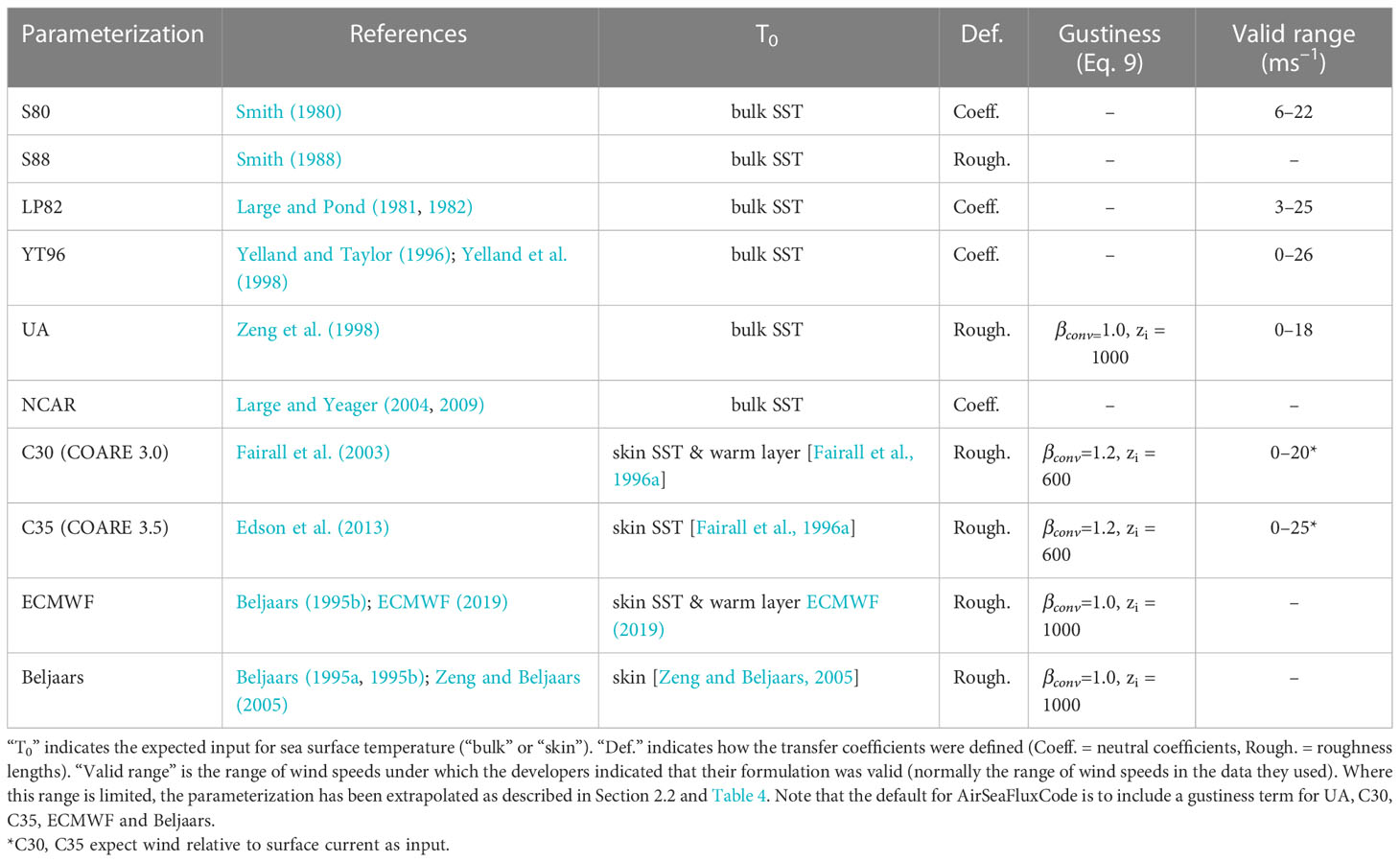
Table 1 Summary of parameterizations implemented in AirSeaFluxCode as documented or implemented by the parameterization developers.

This paper is structured as follows. Section 2 gives an overview of the parameterizations and describes the AirSeaFluxCode package. Section 3 compares the implementation of parameterizations in the AirSeaFluxCode to code provided by algorithm developers, and quantifies the effect of various implementation choices on the resulting fluxes and on the height- and stability-adjusted meteorological variables. Our conclusions, recommendations and development plans for AirSeaFluxCode form Section 4.

We use the term “parameterization” to refer to the combination of transfer coefficients, roughness lengths and stability parameters. We use “algorithm” to refer to the combination of the parameterization and the full calculation process or implementation. To aid discussion of the results we have provided a set of “significance” values chosen according to the above requirements for flux uncertainty along with an assessment of reasonable measurement uncertainties for the bulk variables, see Table 2.

TABLE 2

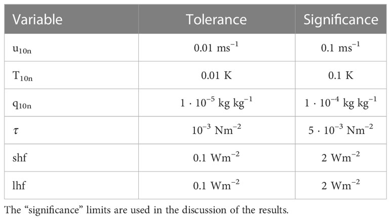
Table 2 “Tolerance” are the default values used to test for convergence.

We follow the convention of a positive flux being a gain by the ocean, so incoming shortwave radiation is positive and the other heat flux components are usually negative (representing a heat loss by the ocean). A positive wind stress represents momentum transfer from the atmosphere into the ocean.

2 Method

2.1 Summary of air-sea interaction theory

The AirSeaFluxCode software package calculates TSF from bulk measurements or other estimates of meteorological variables (near surface wind speed, air temperature, humidity) and sea surface temperature. We refer to these collectively as surface state variables (SSV) following Brodeau et al. (2017). Here we provide a brief overview of relevant air-sea interaction theory to enable an understanding of the parameterizations and the output parameters. A fuller description can be found in textbooks such as Stull (1988) or Kraus and Businger (1995).

The parameterizations differ in several different ways, including: the functions used to account for variations in near surface atmospheric stability (Section 2.2, Table 3); the values of the transfer coefficients (Section 2.2.1, Figure 1 and Table 4); the functions to calculate roughness lengths (Figure 1 and Table 5); whether the effects of convective gustiness are accounted for (Section 3.2.6, Table 1, Section S4, Table S2); the choice of the type of surface water temperature variable required as input (Table 1, Section 3.2.5); and the definition of thermodynamic variables, formulae and constants (Section 3.2.1, Table S1). The air-sea fluxes of wind stress (τ), sensible heat flux (shf) and latent heat flux (lhf) are estimated from mean atmospheric parameters using the bulk formulae:

TABLE 3

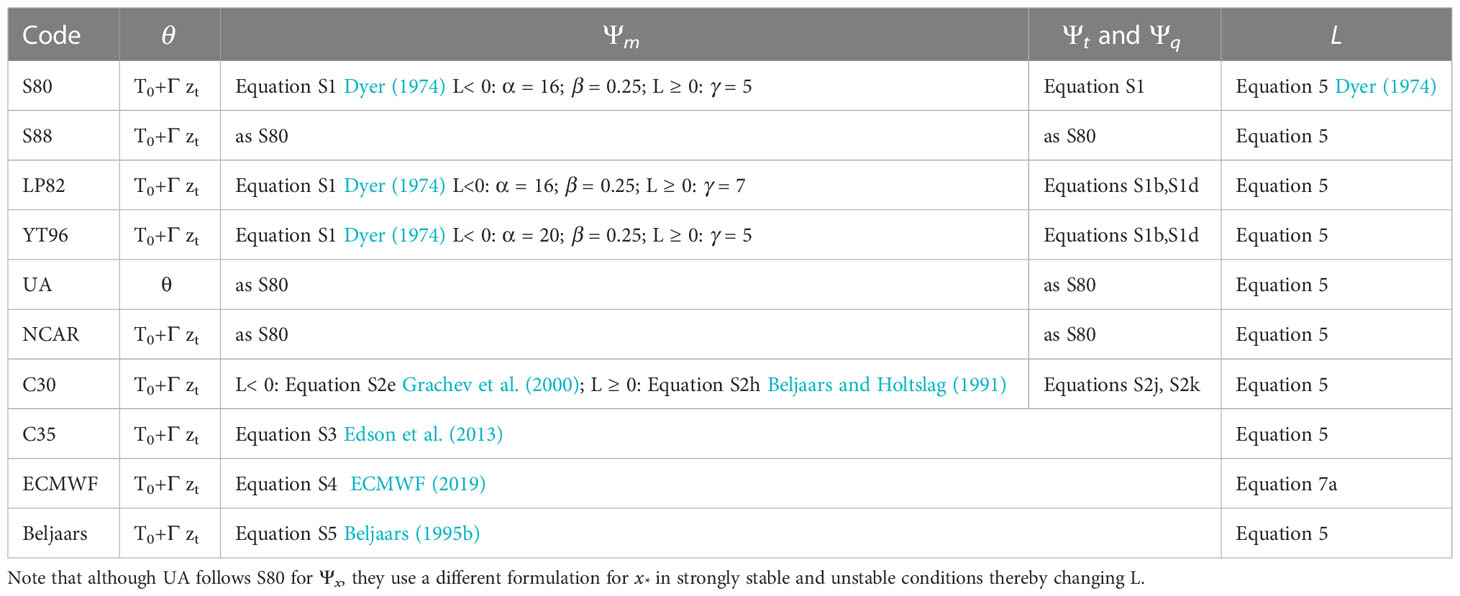
Table 3 Summary of terms used in the algorithms: Potential Temperature [θ (K), where Г is the lapse rate (Table S1)]; Stability functions for momentum (Ψ_m) and temperature (Ψ_t and Ψ_q; the equations are given in Section S6); Monin-Obukhov length [L (m)].

FIGURE 1

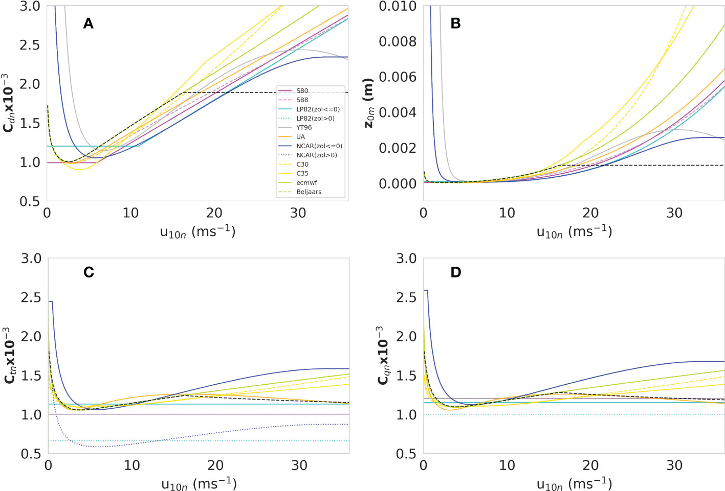
Figure 1 The ten bulk formulae parameterizations included in AirSeaFluxCode as given in the key and Table 1. The momentum flux parameterizations are given in terms of both (A) the drag coefficient at neutral stability and a reference height of 10 m, C_d10n, and (B) momentum roughness length, z_0m, regardless of their original formulation (Tables 4, 5) for ease of comparison. Ten meter neutral transfer coefficients for the (C) sensible heat flux, C_t10n, and (D) the latent heat flux, C_q10n are also shown. Note that LP82 and NCAR both provide different coefficients for the heat fluxes under stable/unstable atmospheric conditions (values for stable conditions are indicated with dotted lines). The dashed black lines show the ECMWF paramaterization as implemented in the Aerobulk code and demonstrates the effect of the limits placed on roughness lengths (these limits are not applied in the AirSeaFluxCode implementation of ECMWF, solid green line).

TABLE 4

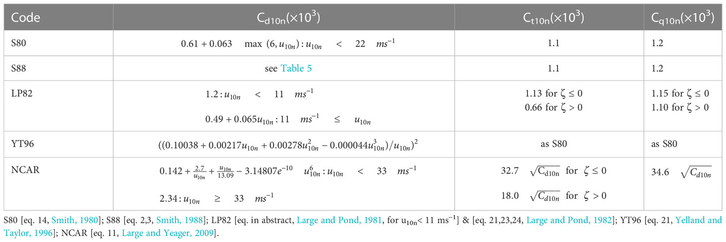
Table 4 Parameterizations defined in terms of the 10 m neutral exchange coefficients.

TABLE 5

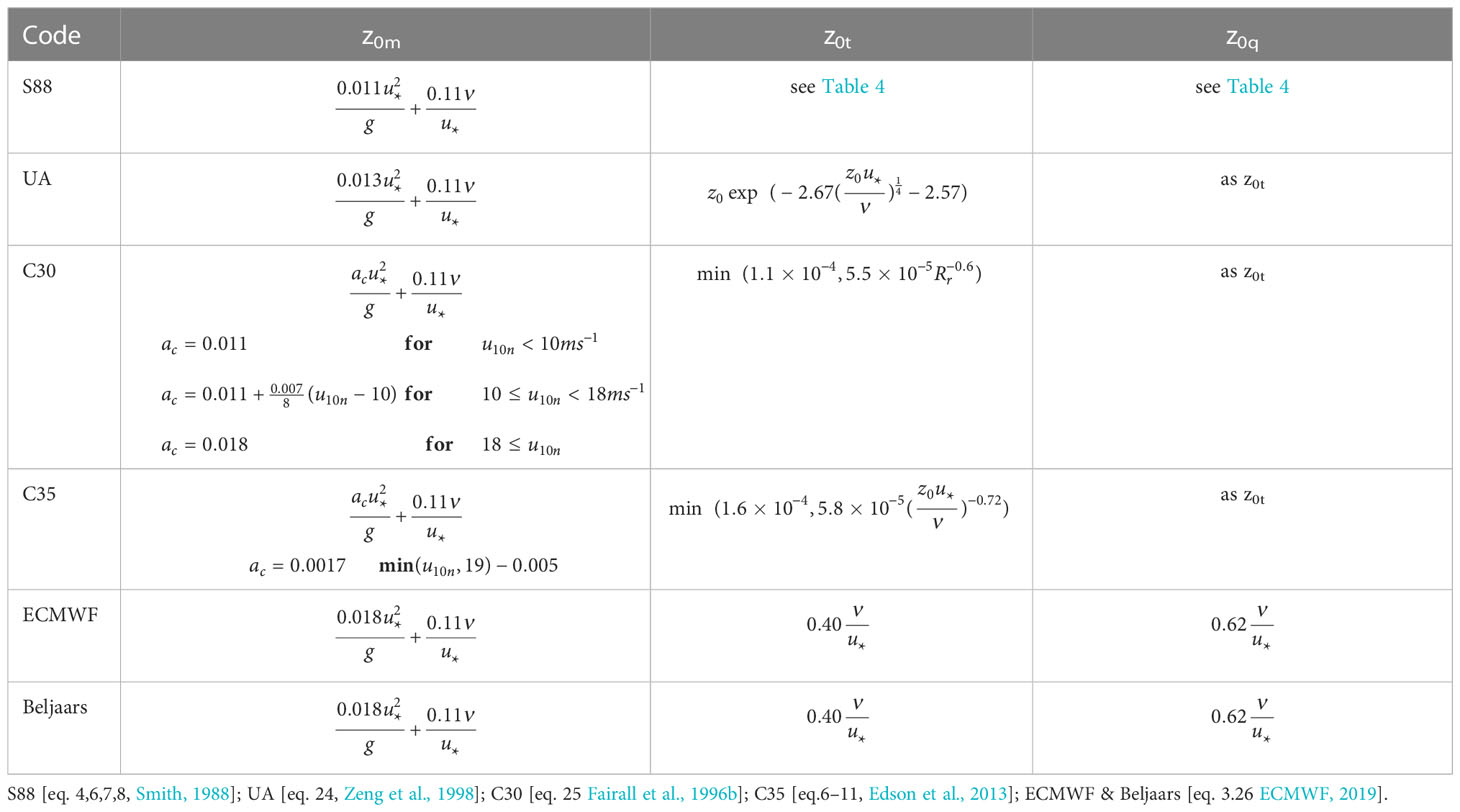
Table 5 Parameterizations defined in terms of the roughness lengths.

$\begin{array}{ll}\tau ={\rho }_0{\text{C}}_{\text{dz}}{\left({\text{u}}_{zm}-u_0\right)}^2& \text{(1a)}\end{array}$

$\begin{array}{ll}\text{shf}={\rho }_0{\text{c}}_{\text{p}}{\text{C}}_{\text{tz}}({\text{u}}_{z_m}-{\text{u}}_0)({\theta }_{{\text{z}}_t} -{\theta }_0)& \text{(1b)}\end{array}$

$\begin{array}{ll}\text{lhf}={\rho }_0{\text{L}}_{\text{v}}{\text{C}}_{\text{qz}}({\text{u}}_{{\text{z}}_m}-{\text{u}}_0)({\text{q}}_{{\text{z}}_q}-{\text{q}}_0)& \text{(1c)}\end{array}$

The transfer coefficients for momentum (C_dz, also known as the drag coefficient), heat (C_tz) and moisture (C_qz) are specific to the input measurement heights z_m, z_t and z_q. ρ₀ is the air density; c_p the specific heat capacity of dry air at constant pressure; L_v the latent heat of vaporisation; u_zm the wind speed at height z_m; u₀ the wind speed at z_0m just above the interface (see Table 5); θ_zt is the potential temperature at height z_t calculated from T_zt the air temperature at measurement (or model level) height z_t by using the dry adiabatic lapse rate (θ_zt=T_zt+Г_zt; Г=g/c_p where g is the acceleration of gravity Busch (1973)); and θ₀ is the potential temperature at height z_0t calculated from T₀ the air temperature at height z_0t; q_zq the specific humidity at height z_q; q₀ the specific humidity at height z_0q. Note that q₀ is calculated from SST as an approximation to the air temperature very close to the surface.

If it is assumed that the fluxes do not vary with height in the atmospheric layer near the ocean surface (the “constant flux layer”, order tens of meters thick), Equations (1) can also be written in terms of vertically invariant scaling parameters: the friction velocity (u_∗), the characteristic potential temperature (θ_*) and characteristic humidity (q_∗), (Equations 2):

$\begin{array}{ll}\tau ={\rho }_0{\text{u}}_{\ast }^2& \text{(2a)}\end{array}$

$\begin{array}{ll}\text{shf}={\rho }_0{\text{c}}_{\text{p}}{\text{u}}_{\ast }{\theta }_{\ast }& \text{(2b)}\end{array}$

$\begin{array}{ll}\text{lhf}={\rho }_0{\text{L}}_{\text{v}}{\text{u}}_{\ast }{\text{q}}_{\ast }& \text{(2c)}\end{array}$

Alternatively the transfer coefficients can be defined in terms of characteristic length scales, known as roughness lengths, z_0m for momentum, z_0t for temperature and z_0q for moisture, (Equations 3):

$\begin{array}{ll}{\text{C}}_{\text{dz}}={\left[\frac{k}{\left(\text{ln }\left(\frac{\text{z}}{{\text{z}}_{0\text{m}}}\right)-{\text{Ψ}}_{\text{m}}\right)}\right]}^2& \text{(3a)}\end{array}$

$\begin{array}{ll}{\text{C}}_{\text{tz}}=\frac{k^2}{\left(\text{ln }\left(\frac{\text{z}}{{\text{z}}_{0m}}\right)-{\text{Ψ}}_{\text{m}}\right)\left(\text{ln }\left(\frac{\text{z}}{{\text{z}}_{0\text{t}}}\right)-{\text{Ψ}}_{\text{t}}\right)}& \text{(3b)}\end{array}$

$\begin{array}{ll}{\text{C}}_{\text{qz}}=\frac{k^2}{\left(\text{ln }\left(\frac{\text{z}}{{\text{z}}_{0m}}\right)-{\text{Ψ}}_{\text{m}}\right)\left(\text{ln }\left(\frac{\text{z}}{{\text{z}}_{0\text{q}}}\right)-{\text{Ψ}}_{\text{q}}\right)}& \text{(3c)}\end{array}$

The stability functions (Ψ_x where x represents either m, t or q) account for the vertical gradients of wind speed, temperature and humidity under different near-surface atmospheric stability conditions. The fluxes both depend on, and modify, these near-surface atmospheric gradients. The atmosphere is typically slightly unstable as the sea is normally warmer than the air just above it. In these conditions turbulence is enhanced, mixing is increased and the vertical gradients are weaker than in neutral conditions. Conversely when the atmosphere is stable, turbulence is suppressed, mixing is weak and steeper gradients can exist. Low wind speed, stable conditions are associated with shallow surface layers as mixing is confined near to the surface: under such conditions the atmosphere at measurement height z (typically 20 m or more on a ship), may be above any constant flux layer and the flux theory will not be valid.

The values for the Ψ_x functions derive from Monin-Obukhov Similarity Theory (e.g. Dyer, 1974) and are estimated from z/L, where L is the Monin-Obukhov Length. Ψ_x is the integral of the dimensionless gradients in the atmosphere (ϕ_x, Equations 4) (Bradley and Fairall, 2006). The form of the dimensionless gradients, and hence the stability functions, varies between the different parameterizations (see Section S2, Table 3). The stability functions for the different parameterizations (Figure 2) are similar in unstable or near-neutral conditions, but markedly different for very stable conditions (roughly, z/L > 2).

FIGURE 2

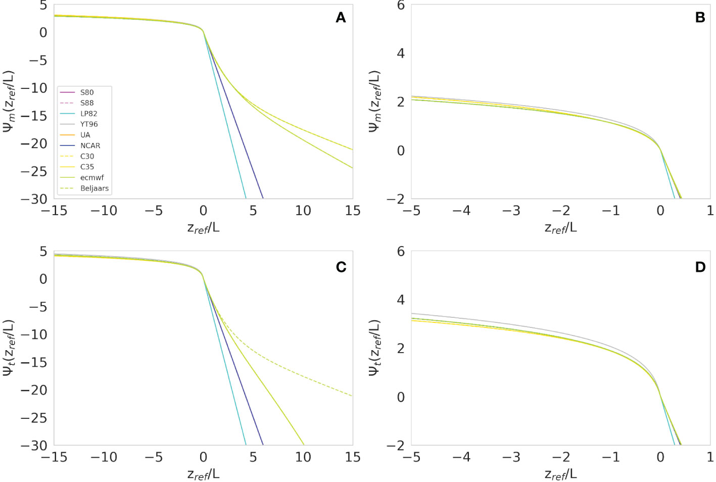
Figure 2 Stability functions versus z_ref/L_tsrv (A, B) for momentum, Ψ_m, and (C, D) heat, Ψ_t, for all bulk parameterizations provided in AirSeaFluxCode. Panels b and d are zoomed in to show the ranges of unstable conditions more clearly. Note that we have used z_ref=10 m.

$\begin{array}{ll}{\varphi }_{\text{x}}=\frac{kz}{{\text{x}}_{*}}\frac{\partial \overline{x}}{\partial z}& \text{(4a)}\end{array}$

$\begin{array}{ll}{\text{Ψ}}_{\text{x}}={\displaystyle {\int }_{{\text{z}}_{0\text{m}}}^{\text{z}}\frac{1-{\varphi }_x}{z}d\text{z}}& \text{(4b)}\end{array}$

In AirSeaFluxCode there are two options to calculate the Monin-Obukhov length (L). The first (L_tsrv) follows e.g. Smith (1980):

$\begin{array}{ll}\frac{z}{L_{\text{tsrv}}}=\frac{z\left(gk{T}_{*v}\right)}{T_{v10n}{u}_{*}^2}& (5)\end{array}$

where u_* (and similarly for θ_*  and q_∗) is calculated from Equations 6 (which are derived from Equations 1 and 2). T_*v is the scaling parameter for virtual temperature (T_v) estimated as in Equation 6d:

$\begin{array}{ll}{\text{u}}_{*}=\sqrt{{\text{C}}_{\text{dz}}}\left({\text{u}}_{{\text{z}}_m}-{\text{u}}_0\right)& \text{(6a)}\end{array}$

$\begin{array}{ll}{\theta }_{*}=\frac{{\text{C}}_{\text{tz}}}{\sqrt{{\text{C}}_{\text{dz}}}}\left({\theta }_{{\text{z}}_t}-{\theta }_0\right)& \text{(6b)}\end{array}$

$\begin{array}{ll}{\text{q}}_{*}=\frac{C_{qz}}{\sqrt{C_{dz}}}\left({\text{q}}_{{\text{z}}_q}-{\text{q}}_0\right)& \text{(6c)}\end{array}$

$\begin{array}{ll}{\text{T}}_{*\text{v}}={\theta }_{*}\left(1+0.6077q_z\right)+0.6077\theta q_{*}& \text{(6d)}\end{array}$

The second option (L_Rb) is a function of the bulk Richardson number (R_b, defined following [ECMWF, 2019, their equations 3.23–3.24]:

$\begin{array}{ll}\frac{z}{{\text{L}}_{\text{Rb}}}=R_b\frac{{\left[\ln \left(\frac{z+z_{0m}}{z_{0m}}\right)-{\Psi }_m\left(\frac{z+z_{0m}}{L_{\text{Rb}}}\right)+{\Psi }_m\left(\frac{z_{0m}}{L_{Rb}}\right)\right]}^2}{\left[\ln \left(\frac{z+z_{0m}}{z_{0t}}\right)-{\Psi }_t\left(\frac{z+z_{0m}}{L_{Rb}}\right)+{\Psi }_t\left(\frac{z_{0t}}{L_{Rb}}\right)\right]}& \text{(7a)}\end{array}$

$\begin{array}{ll}{R}_b=\left(\frac{g}{{\theta }_v}\right)\frac{z\left({\theta }_{vz}-{\theta }_{v0}\right)}{|u_{zt}{|}^2}& \text{(7b)}\end{array}$

where θ_vz and θ_v0 are the virtual temperatures at level z and at the surface, θ_v is an estimate of virtual potential temperature within the surface layer (here at z_t), and u_zt is the wind speed estimated at height z_t.

The SSV adjusted to a height z_out can be calculated either from surface values (“bottom-up”) using roughness lengths, scaling parameters and the stability functions Ψ_x (Equation 8a), or equivalently by adjusting the measured SSV (“top-down”) using just the scaling parameters and stability functions (Equation 8b). The values of the SSV that would have produced the same values of the scaling parameters (or equivalently surface roughness) in a neutral atmosphere, usually at a 10 m reference height, are referred to as “neutral values” (subscript n) and are given by either Equation 8c (“bottom-up”) or 8d (“top-down”).

$\begin{array}{ll}{x}_{zout}=x_0+\frac{x_{*}}{k}\left(\text{ln}\left(\frac{z_{out}}{z_{0x}}\right)-{\Psi }_x\left(\frac{z_{out}}{L}\right)\right)& \text{(8a)}\end{array}$

$\begin{array}{ll}{x}_{zout}=x_z-\frac{x_{*}}{k}\left(\ln \left(\frac{z_x}{z_{out}}\right)-{\Psi }_x\left(\frac{z_x}{L}\right)+{\Psi }_x\left(\frac{z_{out}}{L}\right)\right)& \text{(8b)}\end{array}$

$\begin{array}{ll}{x}_{10n}=x_0+\frac{x_{*}}{k}\text{ln}\left(\frac{10}{z_{0x}}\right)& \text{(8c)}\end{array}$

$\begin{array}{ll} x_{10n}=x_Z-\frac{x_{*}}{k}\left(\text{ln}\left(\frac{z_x}{10}\right)- {\text{Ψ}}_x\left(\frac{z_x}{L}\right)\right)& \text{(8d)}\end{array}$

At low mean horizontal wind speeds scalar TSF (i.e. sensible and latent heat) may be driven largely by vertical convective gusts. This is sometimes accounted for by including a gustiness term (u_g in ms^–1) added in quadrature to the horizontal wind components (Fairall et al., 1996b), (Equation 9, Section S4).

$\begin{array}{ll}{\text{u}}_{\text{g}}=\{\begin{array}{ll}\mathit{max}\left({\text{u}}_{{\text{g}}_{\text{min}}},{\beta }_{\text{conv}}(-\frac{g}{T}{\text{u}}_{*}{\text{T}}_{*\text{v}}{\text{z}}_{\text{i}}{)}^{\frac{1}{3}}\right)\hfill & \text{unstable or neutral conditions}\hfill \\ {\text{u}}_{{\text{g}}_{\min }}\hfill & \text{stable conditions}\hfill \end{array}& (9)\end{array}$

where β_conv is an empirical constant and z_i is an estimate of the boundary layer height, u_gmin is the minimum gust wind speed used for all stabilities. For those algorithms that originally included a gustiness term, the values of β_conv and z_i are given in Table 1. The application of the gustiness term is not appropriate to all parameterizations, particularly those that were developed without it, since the impact on the TSF can be very large (Section 3.2.6). Details on how gustiness term is applied are given in Section 2.3.

Some developers remove the effects of gustiness from some of the output parameters, but there is no consensus as to how to do this. Therefore in AirSeaFluxCode the user is provided with options to remove the effects of gustiness from some, all, or none of the TSF and u_10n and u_zout (details in Section S4 and summarized in Table S2). Note that the “bottom-up” (Equations 8a and 8c) and “top-down” (Equations 8b and 8d) approaches to height adjustment produce slightly different results when the gustiness term is included.

The algorithms require as input an estimate of the temperature of the sea surface. Some are designed for use with a bulk water temperature (typically made at depths of 1 to 10 m), whereas others require radiometric “skin” temperature, referred to here as the “cool skin” (Donlon et al., 2002). These measures are not interchangeable, and each parameterization should be used with the measure of sea temperature used in its derivation. See Section 3.2.5 and Table 1.

Finally, many of the parameterizations discussed here are based on direct measurements of the fluxes along with measured, earth-relative wind speed, therefore such parameterizations require earth-relative winds as input. In these cases, the effects of surface currents are implicitly included in the parameterization. This might be reasonable for local wind-driven currents but in regions where strong surface currents are not aligned with the prevailing winds, use of these parameterizations with earth-relative winds introduces additional uncertainties. In contrast, some parameterizations (e.g. C30 and C35) assume winds are relative to the ocean surface: in this case the user should input surface-relative winds.

2.2 AirSeaFluxCode calculation methodology

2.2.1 Transfer coefficients

Transfer coefficients are defined in one of two ways. Either the value of the coefficient at 10 m and in neutral atmospheric conditions is specified, or a roughness length is specified (z_0m for momentum, z_0t for temperature and z_0q for moisture) (see Table 1). For the latter, transfer coefficients are calculated from the roughness lengths (Equations 3), and vice versa for the former.

Most of the uncertainty in the estimated TSF is due to the wide range of values assigned to the transfer coefficient or roughness lengths particularly at high and low wind speeds (Figure 1), since differences in the fluxes are directly proportional to differences in the transfer coefficients (Equation 1). It should be noted that LP82 and NCAR (based partly on LP82) define separate heat transfer coefficients for unstable and stable conditions.

The drag coefficients, and some parameterizations of the heat transfer coefficients, vary with wind speed (Tables 4, 5). Some parameterizations (S80, LP82) were originally defined for the limited wind speed range over which direct measurements of the fluxes were obtained in the observational programs. These ranges are listed in Table 1. To apply these parameterizations to all wind speeds we have extrapolated the coefficient definitions at both low and high wind speeds (Table 4). YT96 provided a drag coefficient in terms of u_*: we convert their Equation 21 to a drag coefficient and extrapolate this at high wind speeds. This extrapolation, based on a polynomial fit, results in drag coefficients that decrease for winds over 30 ms^–1, and the authors advised against extrapolation. However, subsequent evidence (e.g. Powell et al., 2003) supports such a decrease up to ~ 50 ms^–1 and we therefore use this extrapolation here.

2.2.2 Algorithm implementation

In AirSeaFluxCode we use a consistent calculation approach across all parameterizations: where this differs from published descriptions or developer-provided code the effect of those differences on estimates of the fluxes or height-adjusted SSV are quantified (see Section 3.1, Table 6). AirSeaFluxCode estimates the transfer coefficients at the measurement height(s) and the stability-dependent flux profiles using an iterative method (Large, 1979). The flux profile relationships assume that the variable being mixed is conservative, and the adiabatic variations with pressure are accounted for using an approximate relationship for potential temperature [θ_zt ≈ T_zt + Г_zt Busch (1973), where Г is the adiabatic lapse rate (Table S1)]. A schematic of AirSeaFluxCode’s implementation is shown in Figure 3.

TABLE 6

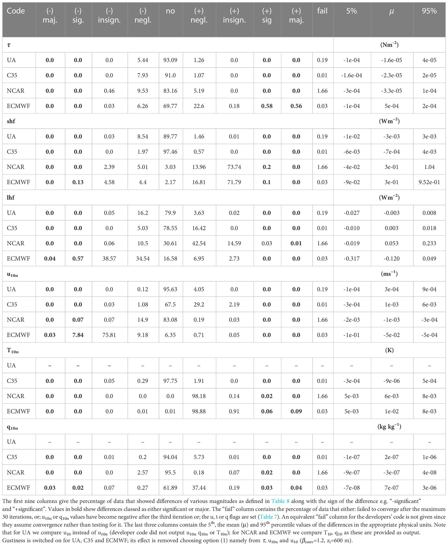
Table 6 Comparison of TSF and adjusted SSV results with those from existing software (ΔX = X_{AirSeaFluxCode}-X_Developers’).

FIGURE 3

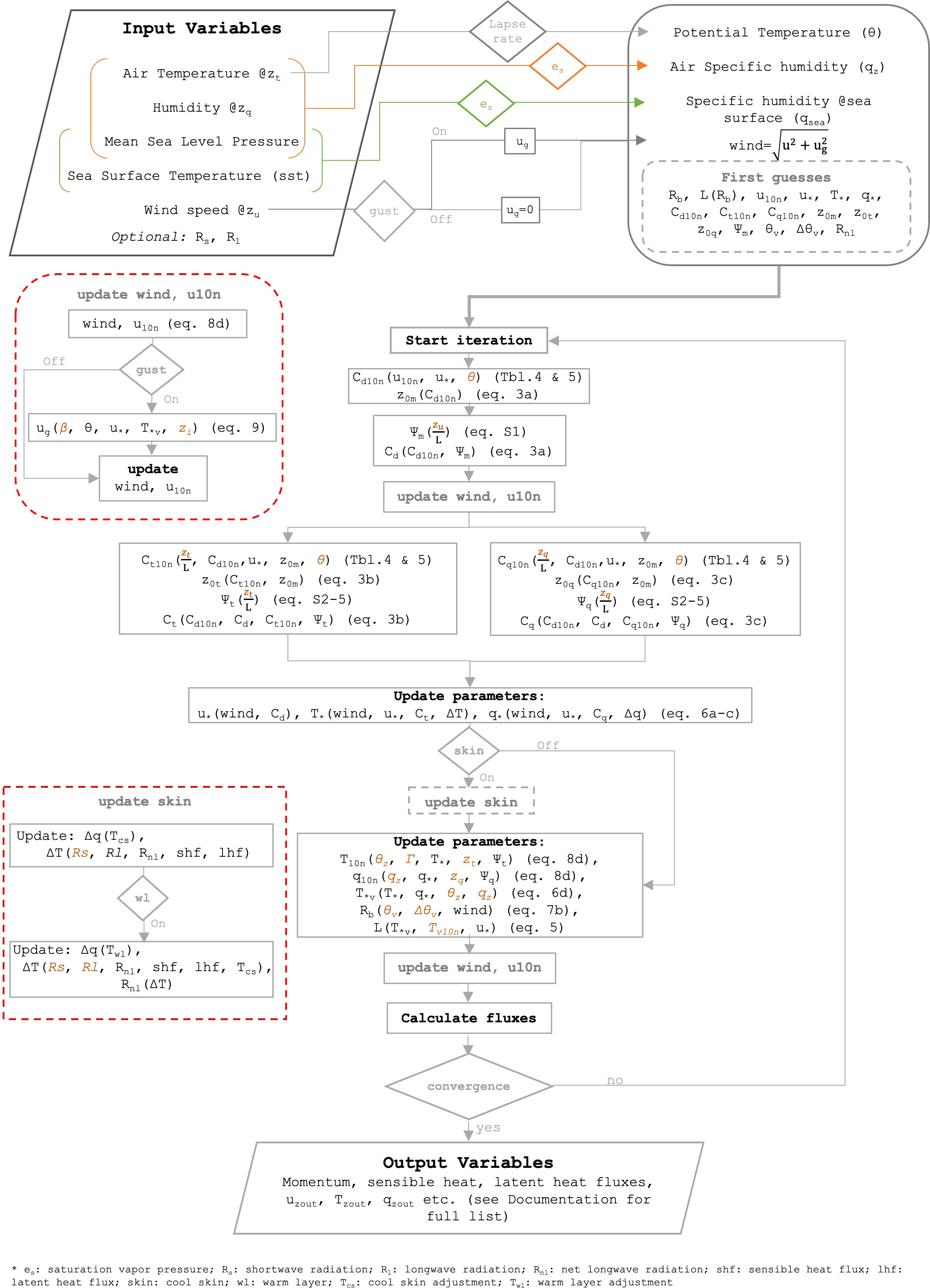
Figure 3 Schematic of AirSeaFluxCode’s implementation. The main dependencies for each variable are shown in parenthesis. Inside the parenthesis variables that are not updated during the iteration are shown in colored italics.

The user-defined output height (z_out) can be different from the reference height of 10 meters used for the definition of coefficients (see Section 2.2.1). In this paper we use 10 m for both, giving outputs of u_10n and u₁₀ (and similarly for T and q). The code calculates values at the output and reference heights top-down (Equations 8b and 8d). u₀ is not include in AirSeaFluxCode, equivalent to neglecting surface currents.

To initialize the flux calculation potential temperature at the measurement height is calculated and 10 m neutral values of the SSV are approximated by the measured values. If the specific humidity of air (q_zq) is not available it can be calculated from relative humidity (RH) or dew point temperature (T_d) using the saturation vapour pressure function (e_s, Section S5) selected by the user. The saturation specific humidity at the sea surface (q₀) is calculated at the sea surface temperature applying a 2% salt reduction (Section 3.2.4). A first guess of z/L is calculated following Grachev and Fairall (1997) using the following Equations 10:

$\begin{array}{ll}\frac{z}{L}=12R_b& \text{(10a)}\end{array}$

$\begin{array}{ll}{R}_b=\frac{g}{T_{z_t}}\frac{z_t\Delta T_v}{u_{z_m}^2}& \text{(10b)}\end{array}$

These approximations allow the calculation of C_dn and z_0m (Tables 4, 5) and friction velocity (u_*, Equation 6a). Next Ψ_x (Table 3, Section S2) can be estimated to give C_d, C_t and C_q (Equations 3).

The iteration follows the flow chart in Figure 3. If options for the calculation for gustiness or cool skin/warm layer are activated these are updated for each step.

AirSeaFluxCode tests for convergence between the current and previous iteration step by using the default tolerance limits shown in Table 2 for six variables in total: SSV adjusted to 10 m and to neutral stability (u_10n, T_10n, q_10n) and the calculated TSF (τ, shf, lhf). These default tolerance limits are set according to the minimum uncertainty that is considered feasible for each variable. The user can change the tolerance values and can also choose to test for convergence using only the TSF, or only the SSV. After convergence is achieved the height adjusted values of wind speed, temperature and specific humidity at the user defined output height (z_out) are calculated (Equation 8b). The application of the dry adiabatic lapse rate is reversed after convergence to give T_zout. If convective gustiness was switched on, its effects will be treated according to the user’s choice (selecting one of the options in Table S2) to remove it or not from the output TSF, u_10n and u_zout as described in Section S4.

The number of iterations before convergence is provided as an output (-1 indicates non-convergent points) and any values that have not converged after a user-defined maximum number of iterations have a flag “i” set (Table 7) and are set absent (NaN) unless the user requests their output. Any un-physical values of the adjusted SSV are flagged (details on all flag definitions can be found in Table 7).

TABLE 7

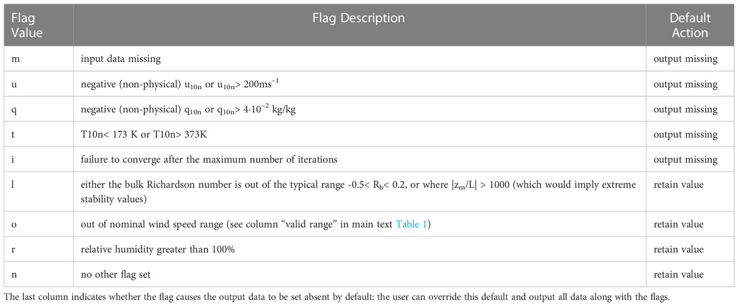
Table 7 Summary of quality control flags provided as output in AirSeaFluxCode.

2.3 AirSeaFluxCode: input parameters, assumptions, user options, and outputs

AirSeaFluxCode can be used with different sources of SSV, e.g. in situ data, satellite retrievals, model output (typically atmospheric reanalyses). In each of these cases different input parameters will be available, and this should be taken into account when selecting which parameterization to use. Typically the parameterizations have been derived from direct flux measurements made using sample periods of order 30 minutes. Any calculations based on data averaged over much longer, or much shorter periods will be more uncertain (Ledvina et al., 1993; Gulev, 1994; Cronin et al., 2006).

The parameterizations vary in complexity with some requiring additional input parameters (e.g. downwelling radiation) and some including additional terms in the calculation (e.g. convective gustiness) in an attempt to better represent the physics of air-sea exchange and/or improve the stability of the iterative calculation. Whilst some of these additions may improve algorithm performance any uncertainty in the additional parameters or terms will affect the results (Bradley and Fairall, 2006; Cronin et al., 2019). In AirSeaFluxCode we have included parameterizations where sea state was optional (but AirSeaFluxCode does not currently incorporate the option).

The minimum set of input SSV required for AirSeaFluxCode to calculate momentum and sensible heat fluxes are near surface wind speed, air temperature and sea surface temperature. Near surface humidity is also required to calculate latent heat flux. Depending on the type of humidity data available, an estimate of atmospheric pressure may also be required to calculate specific humidity. Implementation of skin temperature or warm-layer adjustments require additional parameters such as radiation. If these parameters are not available from the main data source, it may be possible to use estimates from other sources, e.g. climatology, gridded products or atmospheric reanalysis. The uncertainty in the calculated fluxes will depend on their sensitivity to each SSV and its uncertainty.

The basic definitions of each parameterization are summarized in Tables 1–5. Details of the calculation, including information on meteorological parameters such as the density of air or latent heat of vaporisation, can be found in Table S1 and in the AirSeaFluxCode Documentation [https://git.noc.ac.uk/NOCSurfaceProcesses/AirSeaFluxCode].

The input requirements, assumptions made, user options, and outputs are:

● Inputs required:

- wind speed, near surface air temperature, sea surface temperature and the type of SST (skin or bulk) are required for momentum and sensible heat fluxes. Note that C30 and C35 require wind speed and direction relative to the surface currents (rather than ground-relative) and our algorithm assumes that the necessary calculation has been performed by the user prior to input

- humidity must be input for lhf to be calculated; input humidity variable can be specific humidity (q), RH or dew point temperature (T_d)

- measurement heights are required for wind speed, air temperature, and humidity (if input)

- sea level pressure is a recommended input since it improves the accuracy of the output TSF

- if relative humidity (RH) is provided and sea level pressure is missing a default value of 1013 hPa is used (the user can provide an alternative estimate)

- choice of parameterization

- if calculating the cool skin or warm layer adjustments (when the parameterization is expecting a skin SST and the available input is bulk SST), estimates of downwelling shortwave and longwave radiation are required

- the latitude (for calculating acceleration due to gravity); if not provided a value of 45°N is used.

● User options for:

- The saturation vapor pressure function (e_s) used in humidity calculations, the default is Buck (2012). Other options are available and these are discussed in Sections 3.2.3, S5.

- The convective gustiness term, by default it is turned off except for those parameterizations that originally implemented it, i.e. UA, C30, C35, ECMWF and Beljaars.

  * The gustiness term is automatically turned on if the UA, C30, C35, ECMWF or Beljaars parameterizations are chosen and the values of the gustiness parameters (β_conv, z_i, u_gmin in Equation 9) are automatically set to 1.2, 600 m, 0.01 ms^–1 respectively. By default, the effects of gustiness are removed from τ, u_10n and u_zout following the approach taken by Fairall et al. (2003) (option (1) below and Table S2).

  * The user can over-ride the above defaults and choose to set gustiness on/off for any given parameterization. If the user switches gustiness on they must provide values for β_conv, z_i, u_gmin, and also select one of six options to remove the effects of gustiness from the output parameters using the gustiness factor (GF, the ratio of the gusty wind to measured wind, see Table S2), i.e

    option 1: apply GF to τ, u_10n and u_zout (as in Fairall et al. (2003) documentation for C35)

    option 2: apply the GF to all TSF, u_10n and u_zout

    option 3: do not remove the effects of gustiness from any parameter (i.e. GF = 1)

    option 4: apply GF only to τ (as in ECMWF code)

    option 5: similar to (option 1), but using Equations S8d, S9d for the SSV (as in UA code)

    option 6: similar to (option 1) but following the developers’ code for C35 rather than the C35 documentation

- The Monin-Obukhov length (L), calculated either using Equation 5 (default) or Equation 7a, see Section 3.2.2.

- The cool skin adjustment to calculate skin SST from input bulk SST. Three options are given when switched on: Fairall et al. (1996a) (default for C30, and C35), Zeng and Beljaars (2005) (default for Beljaars), ECMWF (2019) (default for ECMWF), see Section 3.2.5.

- The warm layer adjustment; if the cool skin adjustment is switched on, there is an option to additionally switch on a warm layer adjustment (ECMWF, 2019) (switched off by default).

- A SST flag; if the parameterization and type of sea temperature are incompatible (e.g. S80 selected with skin temperature indicated) the code will provide an error message and stop.

- The maximum number of iterations, the default is 30, and we recommend caution in reducing this below 10 (Section 3.2.7).

- The tolerances used to determine if convergence has been achieved and exit the iteration. Tolerance limits (Table 2) can be defined either for the fluxes, or for the height-adjusted parameters, or both (default).

- Convergence; by default non-converging values are set missing (NaN), but there is an option to output all values regardless of convergence and/or the presence of non-physical values for u_10n, q_10n or T_10n (see Table 7).

- The user can specify the desired output height (z_out) for the height adjusted parameters (default is 10 m)

● Outputs include:

- turbulent surface fluxes (τ, shf, lhf, Equations 1)

- wind speed, air temperature and air specific humidity adjusted to the user-specified output height (z_out, Equations 8b)

- wind speed, air temperature and air specific humidity adjusted to 10 m and neutral atmospheric conditions (Equation 8d)

- neutral transfer coefficients at 10 m and stability-dependent transfer coefficients at input height(s) (Equations 3), scaling parameters, stability functions (at measurement height and at z_out) (Equations 2), roughness lengths (Equations 3)

- the Monin-Obukhov length (Equation 5 or 7a), bulk Richardson number (Equation 7b), potential temperature

- if gustiness was switched on, gust wind speed (Equation 9), GF, and u_*gust which includes the gust effect are output

- if the cool skin/warm layer calculations are used then net longwave radiation; temperature and humidity differences due to cool skin/warm layer effect; and the thickness of the viscous skin layer (Fairall et al., 1996a; ECMWF, 2019) are output

- quality control flags, see Table 7 for details

A full list of output variables is given in the documentation supplied with AirSeaFluxCode (Section S1). The user can calculate other variables, such as evaporation, by selecting the full range of output parameters. Alternatively the user can choose a “limited” output (TSF, SSV at z_out) or a user-defined set of output variables.

3 Results

There are two different test data sets available in the AirSeaFluxCode’s repository, one based on observations from research vessels provided by the Shipboard Automated Meteorological and Oceanographic System (SAMOS, Smith et al., 2018; Smith et al., 2019) and the other sub-sampled from global hourly ERA5 (Hersbach et al., 2018; Hersbach et al., 2020), see Section S6. All the results presented in this paper use the ERA5 (Hersbach et al., 2018) test dataset which provides global coverage, a very wide variety of conditions and a full set of SSV.

In describing our results we use the following classifications (see Table 8): No effect<0.1 × tolerance (Table 2); negligible effect<tolerance; insignificant effect < significance level (Table 2, Section 1.1); significant effect<5 × significance; otherwise a major effect. Note that while some differences may be classed as significant or major, they may actually represent a fairly small percentage of the SSV or TSF itself. When larger differences are encountered we therefore consider them both as actual differences and as percentages. In some cases, we discuss differences that are classed as insignificant (based on requirements for climate applications, Section 1.1) if these differences are either unexpected or result in a systematic bias.

TABLE 8

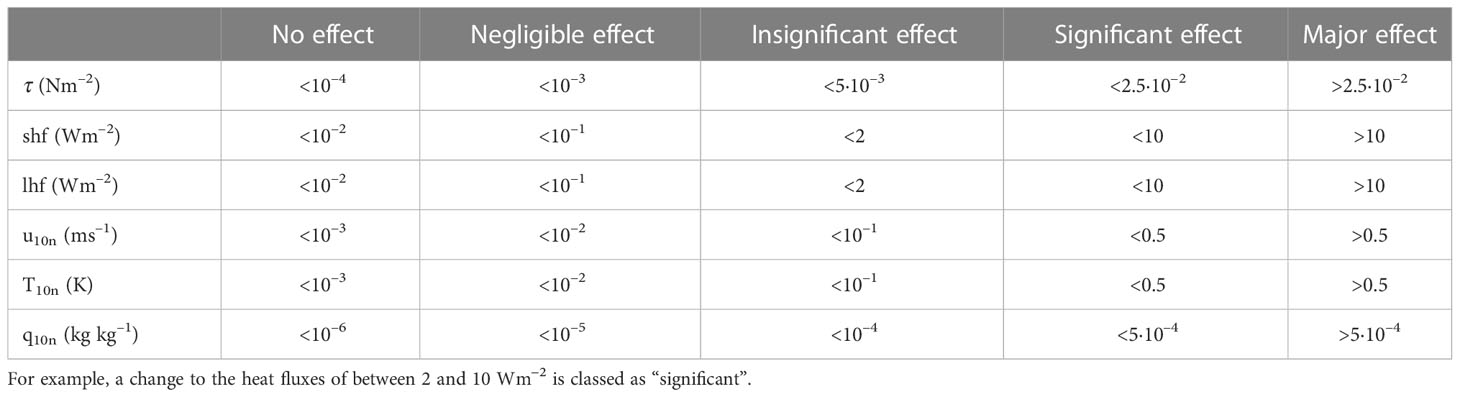
Table 8 Definition of the terms used to describe changes to TSF and SSV.

The value of the air-sea temperature difference (ΔT=T_zt-T₀) is used as an indication of atmospheric stability in the discussions below. ΔT is positive in stable conditions and negative in unstable conditions.

3.1 Comparison of AirSeaFluxCode with existing software

In this section we compare the TSF, and height- and stability-adjusted SSV output from AirSeaFluxCode with those output from four publicly available algorithms, i.e.

- UA (Zeng et al., 1998, https://seaflux.org/seaflux_data/CODE/UA/) in FORTRAN

- COARE 3. 5 (“C35” Fairall et al., 2003; Edson et al., 2013, ftp1.esrl.noaa.gov/BLO/Air-Sea/bulkalg/cor3_5 in MATLAB (MATLAB, 2018))

- NCAR (Large and Yeager, 2004; Large and Yeager, 2009, ncar ocean fluxes.f90, https://data1.gfdl.noaa.gov/nomads/forms/core/COREv2/code_v2.html). We combined the original code with that of AeroBulk’s implementation (Brodeau et al., 2017)

- ECMWF (ECMWF, 2014): we use AeroBulk’s implementation Brodeau et al., (2017) as a proxy

The results of the comparison are summarized in Table 6. Differences in implementation between AirSeaFluxCode and the developer code are described in the Supplementary Material Sections S7.1 - S7.5.

Note that in both AirSeaFluxCode and in the original developer code we use bulk sea surface temperature as input and the cool skin/warm layer adjustments are switched off even if these are switched on by default in the developer code (see Table 9). This was done in order to focus on any changes in the outputs that resulted from differences in the core flux calculations. The cool skin and warm layer adjustments are considered separately (Sections 3.2.5, S7.3).

TABLE 9

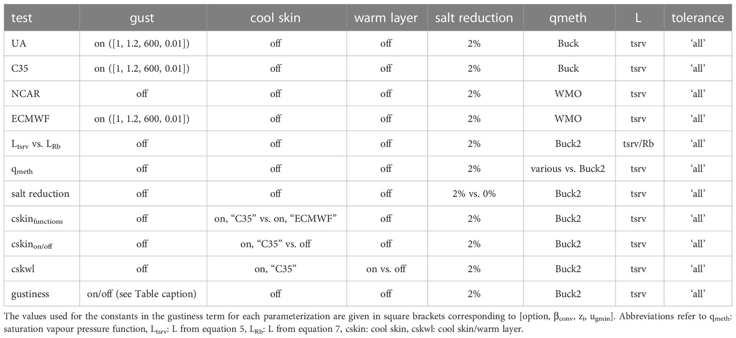
Table 9 A summary of the AirSeaFluxCode input options used in: Section 3.1 - the comparison against the original developer code where available (first four rows); Section 3.2 - test of different formulations for various parameters or optional adjustments (last 7 rows).

For UA, C35 and ECMWF we include a gustiness term following the approach of Fairall et al. (2003) (option (1) Table S2, β_conv=1.2, z_i=600 m, u_gmin=0.01 ms^–1 Equation 9) to remove the effect of gustiness from τ, u_10n and u₁₀. Note that the ECMWF developer code only removes gustiness effects from τ.

For UA and C35 we use relative humidity, calculated from the dew point temperature, as input since that is what the developer code requires. For NCAR and ECMWF the difference in the function used to calculate specific humidity from the input dew point temperature leads to a systematic difference in specific humidity and, in some cases, significant difference in the latent heat flux (Sections S7.4, S7.5). For these algorithms, for the comparison with the developer code we use the values of q_zq and q₀ that are output from Aerobulk as inputs to AirSeaFluxCode so that other differences between the two implementations can be examined.

In the comparisons with the UA and C35 developer code the differences in the TSF and SSV (if available) results are insignificant at most, thus we focus here only on interesting methodological differences. Neither of the developer codes test for convergence whereas in AirSeaFluxCode ~0.2% of data failed to converge for the UA parameterization, and just 0.01% for C35. In both cases these data occurred during low wind speed and stable conditions. Both developer codes apply slightly different methods to the removal of gust effects from u_10n or u₁₀. Rather than applying option (1) as done in AirSeaFluxCode the UA and C35 developer codes apply the equivalent of options (5) and (6) respectively. For UA this has almost no impact on u₁₀ and for C35 the differences are insignificant.

In the comparisons with NCAR (Table 6) significant or major differences in heat fluxes and SSV resulted from a combination of the treatment of thermodynamic variables (c_p and ρ₀) and the methodological differences (number of iterations and ad hoc limits applied to the roughness lengths). For shf 0.2% of differences are classed as significant (the 95^th percentile difference was about 1 Wm^–2, i.e. 3% of the absolute flux) and are positively skewed with the results from the developer code being higher across all wind speeds (by 0.35 Wm^–2 on average). For lhf a small percentage of data shows significant or major differences (0.03%, 0.01% respectively), with a maximum difference of ~15 Wm^–2. All of the major differences in lhf occurred at low wind speeds (below 2 ms^–1) and unstable conditions. In addition, in this comparison we have the highest percentage (1.66%) of data that failed using AirSeaFluxCode due to NCAR’s use of two distinct values for the heat transfer coefficients in stable and unstable conditions (see Section 3.2.7 for details).

For the SSV, the ~0.02% of differences classed as significant in either T₁₀ or q₁₀ occurred under near neutral to stable conditions, while the 0.07% of data with significant difference in u_10n occurs for wind speeds below about 5 ms^–1, mostly under stable conditions for wind speeds below 2 ms^–1.

Table S4 shows another comparison where AirSeaFluxCode was temporarily modified to adopt the NCAR developers thermodynamical options and ad hoc limits. In this case no significant differences were seen in the heat fluxes or SSV, except for just 0.01% of u_10n data. The percentage of data that failed to converge decreases very slightly.

In the comparison with ECMWF we identified differences in methodological, thermodynamical and ad hoc limits in the implementations that can produce significant/major differences in TSF and SSV:

- Most differences are associated with wind speeds greater than 17 ms^–1, and are due to the ad hoc constraint in the Aerobulk code (Figure 1) that limits z_0m to a maximum value of 0.001 m. Over 1% of data showed significant or major differences in τ; about 0.6% showed significant or major difference in lhf; 0.23% showed significant differences in shf.

- ~8% of u_10n data show significant differences across all wind speeds, including 0.03% major differences under low wind speed conditions (< 1 ms^–1). These differences are largely due to the developer code calculating u_10n “bottom-up” with gust included, see Section S7.5 for more details.

Again Table S4 shows a comparison where AirSeaFluxCode was temporarily modified to adopt the Aerobulk developers approach to implementing the ECMWF parameterization, including the ad hoc limits (described in more detail in Section S7.5). Applying the constraint on roughness lengths and stability functions, and using their definitions for c_p and ρ₀, removes all significant differences for the TSF and SSV, apart from u_10n. Applying the same approach to the calculation of the output u_10n (i.e. not removing the effects of gustiness) reduces the significant differences to just 0.01%. See Section S7.5 for further information.

3.1.1 Summary of code comparisons

Comparisons of our code with the original developer code (in a variety of coding languages) for four different parameterizations has shown that the results from AirSeaFluxCode are robust.

In the case of UA and C35 no significant differences were found in the TSF nor in the adjusted SSV (where those data were available as output from the code).

For NCAR, significant differences were seen in a very small fraction (less than 0.1%) of lhf, u_10n, T₁₀ and q₁₀ data, usually under low wind speed conditions. No significant differences were seen in τ. The shf results showed 0.2% significant differences due to the developer’s choice of function for c_p which resulted in a slight high bias in shf across all wind speeds.

For ECMWF, the developers’ use of an upper limit to z_0m had by far the largest impact on the results and caused significant or major differences in all the TSF, particularly at the higher wind speeds. A small number of additional significant differences in the shf were due to the choices for the c_p and ρ₀ parameters.

For most parameterizations, the very small fraction of data that failed to converge in AirSeaFluxCode were obtained under very low wind speed conditions. The exception to this was NCAR, where a relatively large proportion (1.66%) of data failed to converge in near-neutral conditions under moderate and high wind speeds. We examine convergence in more detail in Section 3.2.7).

3.2 Quantification of the effects due to implementation options in the code

In the following subsections we test the impacts of the various implementation choices for: the acceleration of gravity; four thermodynamic variables; the Monin-Obukhov length; saturation vapor pressure; the 2% reduction of saturation specific humidity over the sea surface to account for the effect of salinity; gustiness; cool skin/warm layer adjustments. We use the significance classifications defined in Table 2 and the ERA5-based test data set to examine the impacts of these choices on the fluxes and the height- and stability-adjusted SSV parameters.

The input option combinations used for the various tests are summarized in Table 9. In general, gustiness, cool skin and warm layer options were turned off, except when those options were being tested.

3.2.1 Thermodynamic variables and acceleration due to gravity

The effect of using a constant approximation for gravity, rather than the functional form that depends on latitude (Table S1), was negligible for all output parameters (Table S6). The effect remained negligible when the test was repeated with 1) the ship based data set that contains variable measurement heights (ranging from about 10 m to 31 m) and 2) the reanalysis data setting the measurements heights up to 50 m (not shown).

The calculation of TSF uses several thermodynamic variables which do not always have a definitive method of calculation. Here we compare constant value approximations against the functional dependencies used in AirSeaFluxCode for: specific heat of moist air (c_p) as a function of specific humidity at the sea surface; latent heat of vaporisation (L_v) as a function of sea surface temperature; air density (ρ₀) as a function of pressure and; the dry adiabatic lapse rate (Г) as a function of c_p (see Table S1). Using the constant value approximations significantly affects the TSF in some cases, but not the SSV.

c_p scales the shf (Equation 1b) but the effect on other outputs is negligible (Table S7). In the functional dependence, c_p increases with q₀. Setting c_p to a constant (1020 J kg^–1K^–1, following Brodeau et al. (2017)) means that in regions where specific humidity is relatively high (low) c_p and hence the shf are underestimated (overestimated) compared to the functional form. Up to about 1% of data (depending on the parameterization) show significant differences in shf. Using a different functional form, such as that used in Aerobulk, can also lead to significant differences in shf in up to ~0.1% of data (Table S8) compared to those from AirSeaFluxCode.

L_v scales the lhf (Equation 1c) and the effect on other outputs is negligible (Table S9). Neglecting the functional dependence of L_v on T₀ (L_v decreases with increasing air temperature) and using a constant value of (2.46 · 10⁶ J kg^–1) instead produces significant differences in lhf for about 10% of data. Use of this constant overestimates L_v and hence lhf loss in the tropics by up to 4 Wm^–2 and underestimates it at high latitudes by up to 3 Wm^–2 (Figure S1), with a mean change of about +0.5 Wm^–2 (c.f. +1.1 Wm^–2 in Brodeau et al. (2017)).

ρ₀ varies systematically by nearly 20% across the globe, being lowest in the tropics and highest at high latitudes, and scales all of the TSF (Equations 1). Using a constant ρ₀ of 1.2 kg m^–3 produces major changes in all of the TSF (Table S10). Use of a constant ρ₀ decreases τ by 0.002 Nm^–2 on average: up to 17% of data show a significant change and an additional ~2% show a major change. The maximum values of the changes are order 0.03 Nm^–2, and occur for τ values of 0.57 to 0.69 Nm^–2, i.e. they represent a ~6% change of the flux. For the shf about 6.5% of data show significant changes and a further ~0.3% show major changes. Again the changes are skewed, with the use of a constant value decreasing the heat loss by the ocean. The maximum values of the changes are order -15 Wm^–2, and occur for shf values of -185 to -164 Wm^–2, i.e. they represent a ~9% change of the flux. The impact on the lhf is even greater, with up to 50% of data showing significant changes and a further 2% or more showing major changes. When a constant is used the tropics show an increased heat loss by the ocean of up to 15 Wm^–2, and high latitudes show a decreased heat loss of similar magnitude (Figure 4). These maximum changes occur at wind speeds greater than ~6 ms^–1, a wide range of stability conditions and represent up to a 6% change in lhf (maximum differences occur for lhf ranging approximately from -250 to -230 Wm^–2).

FIGURE 4

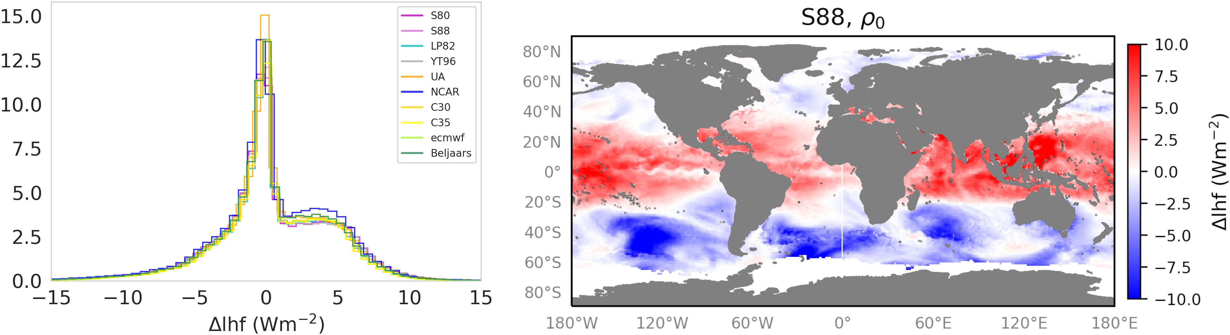
Figure 4 The impact of formulating the density of air (ρ₀) as a constant rather than a function (see Tables S1, S10). Left: histograms of the difference in latent heat flux, Δlhf= lh_ffunction-lh_fconstant (Wm^–2) for the ten parameterizations in AirSeaFluxCode. Right: the global distribution of this difference using the S88 parameterization.

If the different functional form of ρ₀ in Aerobulk is applied then no significant differences are seen, but the heat flux results are slightly skewed (Table S11).

Using a constant value for the dry adiabatic lapse rate Г has no effect on any of the TSF or SSV estimates (Table S12).

3.2.2 Monin-Obukhov length

As described in Section 2.1 AirSeaFluxCode initializes the flux calculation using the bulk Richardson number (Grachev and Fairall, 1997)(Equation 10) but includes two options for the calculation of the Monin-Obukhov length (L, Equations 5 and 7) during the iteration process. Originally, parameterizations S88, LP82, YT96 and NCAR follow the approach taken by S80 of using L_tsrv at every step. UA, C30, C35 and Beljaars calculate L_Rb initially and then iterate using L_tsrv. ECMWF uses R_b throughout. Here we test the use of L_tsrv versus L_Rb in the iteration.

The choice of L formulation on τ and shf leads to no significant differences (see Table S13) for the majority of parameterizations. The exceptions are YT96 where 0.01% of τ values show significant differences; and NCAR and LP82 where just 0.04% and 0.01% of shf results respectively show differences classed as significant. These changes occur under moderate and high wind speeds and very near-neutral conditions and are caused by the use of different heat transfer coefficients for stable and unstable conditions (Section 3.2.7). For the lhf, C30, C35, ECMWF and Beljaars show no significant changes, and the other parameterizations show significant changes in less than 1% of data. Figure S2 shows the small amount of data with significant changes typically occur underlow and moderate wind speeds, with the larger changes tending to occur during stable atmospheric conditions.

The choice of L functions has limited impact on the adjusted SSV u_10n and T_10n. For u_10n significant or major differences affect < 0.1% of the data for all parameterizations. For UA T_10n has < 0.3% significant or major differences and NCAR and S80 ≤ 0.1%. Differences for q_10n are slightly larger again: S80 and S88 have ≤ 1% significant or major differences, UA <1% and others ≤ 0.3%. The resulting z_ref/L stability values are compared in Figure S3. For all parameterizations the vast majority (98% or more) of results lie within the range -5< z/L< +2.

For most parameterizations the choice of L function has little or no impact on the failure rate. However, for LP82 and NCAR the failure rates decrease considerably when L_Rb is used: fail rates decrease from 0.99% to 0.03% for LP82 and from 1.66% to 0.18% for NCAR. For those two parameterizations the high failure rates when using L_tsrv occur for data at moderate and high wind speeds when conditions are near-neutral (Figure S4), conditions under which most algorithms converge after just a few iterations (Section 3.2.7), and are caused by the use of different heat transfer coefficients for unstable and stable conditions. The UA parameterization is the only one to show an increase in failure rate (from 0.26% to 0.47%) when L_Rb is used, since the UA stability functions are particularly sensitive to the value of L.

3.2.3 Formula to calculate saturation vapour pressure

In AirSeaFluxCode q is computed by default from RH or dew point temperature following Buck (2012), an updated version of the widely-used Buck (1981) function to calculate the saturation vapour pressure (e_s). Any required conversion of humidity variable to give q introduces uncertainties as additional variables (e.g. temperature and air pressure) are required.

Section S5 describes the 13 alternative formulations for (e_s) that are included in AirSeaFluxCode. Table S14 examines the impact of using a typical alternative formulation (WMO (2018)) instead of Buck (2012). This has almost no effect on τ and shf, nor on u_10n or T_10n (Table S14). There are no significant changes seen in lhf or q_10n but for these parameters the differences are skewed, with a mean change in the lhf of about 0.2 Wm^–2, i.e. a systematic increase of heat loss by the ocean.

Table S15 examines the impact of all 13 formulations using the S88 parameterization as an example. Nine of the 13 formulations produces no significant differences in the TSF or SSV. Of the rest, the largest differences are seen when the Preining (Vehkamäki et al., 2002) is used instead of Buck (2012). In this case, 0.33% of lhf results show significant differences and the mean change is increased to 0.54 Wm^–2. For more details see Section S5 in the Supplementary Material.

3.2.4 Calculation of q₀ at sea surface

Brunke et al. (2003) and Brodeau et al. (2017) concluded that the accuracy of the estimate of the saturation specific humidity at the sea surface (q₀) is a major source of uncertainty in the computation of TSF. Brodeau et al. (2017) show that the omission of the 2% salinity-related reduction leads to a 5%–10% increase in the lhf from the ocean globally, and that the error can become “substantial” in near-neutral to weakly stratified atmospheric surface layers.

We investigate the effect of ignoring the 2% reduction (Table S16). Neglecting the 2% reduction has no significant effect on τ, shf or T_10n parameters and ≤ 0.04% of data show a significant effect on u_10n. In contrast, the impact on the lhf is dramatic, with more than 90% of data showing significant or major changes: the mean value of the change is ~9 Wm^–2 (c.f. our significance threshold of 2 Wm^–2). The impact on q_10n is slightly less dramatic: roughly 20% of data show significant changes and the mean change is about 0.06 g kg^–1 (c.f. our significance threshold of 0.1 g kg^–1).

Figure S6A shows the frequency distribution of the changes in lhf for all 10 parameterizations: all experience changes that can exceed 20 Wm^–2. Figure S6B uses the S88 parameterization to illustrate the changes in both lhf and q₀ as a function of atmospheric stability as indicated by ΔT. The largest changes occur under near-neutral conditions associated with larger wind speeds (not shown), and hence large absolute values of lhf.

It is no longer common practice to neglect the effect of salinity reduction on q₀: none of the algorithms considered here neglects it but several examined by Brunke et al. (2003) did. However, there is uncertainty around the correct percentage reduction to use: we tested a range of reductions from 1.6% to 2.4% and quantified the effects relative to the typically-used 2% value (Figure S7). The differences occur mainly in the tropics (Figure S7) and are associated with high wind speeds (not shown). Use of a 1.9% or 2.1% value in the salt reduction term produced no significant differences in the lhf data. Reduction values of 1.8% or 2.2% give lhf differences that occasionally exceed our 2 Wm^–2 significance threshold, and reduction values of 1.6% or 2.4% result in significant changes in approximately 50% of the data.

3.2.5 Cool skin and warm layer adjustments

There are diurnally-varying temperature gradients (a “warm layer”) just below the sea surface, particularly under low wind speed and sunny conditions, where temperatures at depth are lower than those closer to the surface. However, at the very surface of the ocean the “skin” (<< 1 mm thick) is typically cooler than the underlying water (Alappattu et al., 2017) (the “cool skin”). It is the temperature contrast across the air-skin interface that will control the exchange of heat. Some parameterizations (e.g. C30, C35, ECMWF, Beljaars) were developed using skin temperatures. To apply these parameterizations using input data that only includes bulk measurements of sea temperature (typically made at depths between about 1 and 10 m) both the warm layer and cool skin adjustment are necessary. These adjustments require measurements that resolve the diurnal cycle (at least hourly, Cronin et al. (2006)) including additional input parameters of short and long-wave radiation and are a very simple representation of rather complex processes and therefore contain substantial uncertainty.

In contrast, many other parameterizations were developed using bulk sea temperature measurements (e.g. S80, S88, LP82, YT96, UA, NCAR). In this case the mean effect of any near-surface gradients (warm layer or skin) is included in the parameterization and neither adjustment should be applied. If the available bulk measurement is at a different depth to that used in the derivation of the parameterization this will add additional uncertainty, but this effect is not usually considered.

The results below demonstrate the dramatic impact of using the “wrong” water temperature measurements, or applying an adjustment to the “wrong” parameterization. As noted above the formulation of the cool skin and warm layer adjustments are themselves uncertain, so the impacts below should be considered indicative. In AirSeaFluxCode the user inputs whether skin or bulk temperature is available: the skin temperature calculation (and optionally the warm layer calculation) is activated if the chosen parameterization requires it (e.g. C35 with bulk temperature indicated). If the parameterization and temperature are incompatible (e.g. S80 selected with skin temperature indicated) the code will provide an error message and stop.

In this section we examine: 1) two different formulations (Edson et al. (2013), and ECMWF (2019)) for the cool skin adjustment (with the warm layer turned off in both cases, see Table S17); 2) the impact of turning cool skin on versus off (with the warm layer turned off in both cases) to illustrate the impact of using the “wrong estimate” for surface temperature T₀ (Table S18); and 3) the impact of turning warm layer formulation on vs off (with the cool skin on in both cases, see Table S19).

For completeness, a direct comparison was made between AirSeaFluxCode and the C35 developer code, both with the skin adjustment turned on to check the implementation of that adjustment in AirSeaFluxCode. No significant differences were seen and more than 99.95% of TSF and SSV data showed merely negligible differences (Table S5).

1. The choice of formulation for the cool skin adjustment (i.e. Edson et al., 2013; ECMWF, 2019, Table S17) results in no significant changes to the calculated τ and almost none to the shf (just 0.01% of data showed significant differences in shf for the ECMWF and Beljaars parameterizations only). For the lhf the results show significant changes (mostly negative) in 1.9% of data or less, resulting in a mean difference of about -0.2 Wm^–2 i.e. a slight decrease in heat loss by the ocean. Less than 0.14% of data show significant changes to u_10n and up to 0.08% show major changes. The impact on q_10n or T_10n affects all or most parameterizations with less than 0.3% of major changes and less than 1.5% of significant changes.

2. Turning the cool skin adjustment off compared to turning it on (ΔX=X_cskinOn-X_cskinOff) has no significant impact on τ but a dramatic impact on the heat fluxes (Table S18). For the shf, about 50% or more data show a significant change: omitting the cool skin effect increases the heat loss from the ocean by about 2 Wm^–2 on average across the whole dataset, with the difference reaching up to ~5 Wm^–2 in the 95^th percentile depending on parameterization. The impact on the lhf is even greater; about 50% of data show significant changes and an additional 15% to 27% of data show major changes. Turning the cool skin adjustment off increases heat loss from the ocean, by ~6 Wm^–2 on average and up to 15 Wm^–2 in the 95^th percentile depending on the parameterization. Figure 5 shows the changes seen in the S88 heat flux results (shf and lhf) against wind speed and ΔT (as an indication of atmospheric stability). The changes in both shf and lhf occur across all wind speeds, and are largest for the more unstable atmospheric conditions.

   Neglecting the cool skin adjustment also impacts the adjusted SSV. For u_10n ~0.7% of data show significant changes, with some parameterizations showing order 0.1% of data with major changes. For T_10n, up to about 10% of data show significant increases, and up to 0.1% show major changes. Neglecting the cool skin adjustment tends to decrease T_10n in the mean. For q_10n, 15 % to 23% of data show significant changes, with up to an additional ~0.5% showing major changes. Again the tendency is to decrease q_10n when the cool skin adjustment is turned off.

Applying the cool skin adjustment has little impact on the failure rates for most of the parameterizations. The failure rates do increase slightly for S80, S88, LP82 and NCAR but these parameterizations were developed for use with bulk T₀ and the application of the cool skin adjustment is not appropriate.

3. Applying the warm layer adjustment also impacts the heat fluxes (Table S19), but to a lesser extent than neglecting the cool skin adjustment. The warm layer adjustment has minimal impact on τ with < 0.03% of data showing significant differences. For the shf, more than 5% of data show significant changes, with a mean increase of heat loss from the ocean of about 0.4 Wm^–2, and a change of -2.5 to -1.7 Wm^–2 in the 5^th percentile depending on the parameterization. The lhf is affected to a lesser extent, with less than 3% of data showing a significant effect. There is a mean increase in heat loss from the ocean of about 0.1 Wm^–2, and changes of up to -1.1 Wm^–2 in the 5^th percentile.

   The warm layer adjustment also affects the adjusted-SSV. For u_10n about 1.5% of data show significant effects, with up to an additional 0.3% showing major effects: the tendency is to increase u_10n, but not significantly in the mean. T_10n and q_10n show similar significant or major changes, with the changes tending to (insignificantly) decrease both parameters on average. Note that applying the warm layer adjustment tends to slightly decrease the impact of the cool skin adjustment, since the former reduces difference between temperatures at depth and at the skin.

FIGURE 5

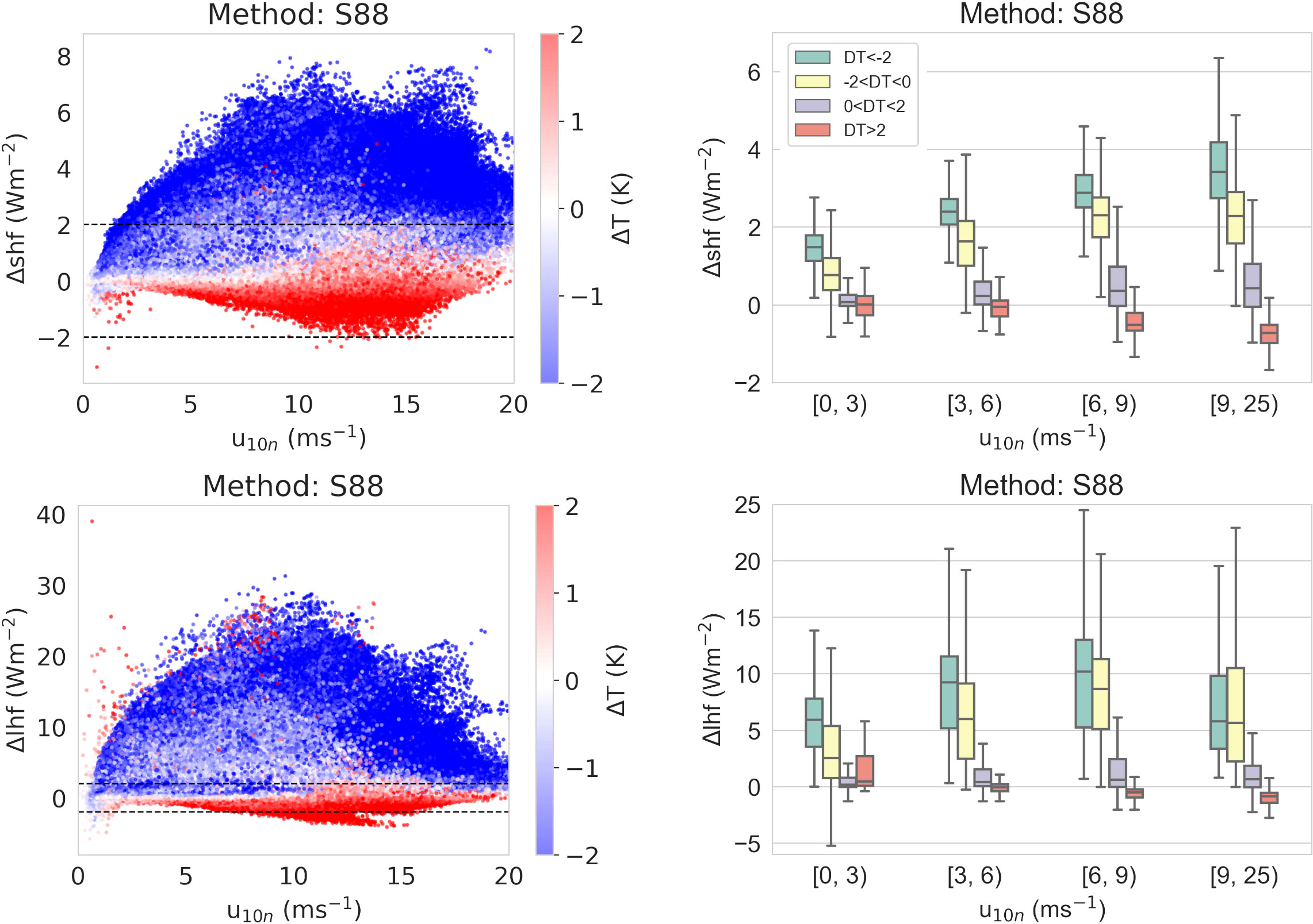
Figure 5 Left hand column: scatterplots of the effect of the cool skin adjustment on shf (top) and lhf (bottom) estimates for S88 bulk parameterization (ΔX=X_skinOn-X_skinOff), relative to u_10n and ΔT. The significance limits (Table 2) for the heat fluxes are denoted by the horizontal dashed lines. Right hand column: the corresponding box-plots of heat fluxes in relation to different ranges of u_10n and ΔT, showing the median (middle line), the inter-quartile range (25–75%, box), and the outer range (whiskers, < 25% and > 75%).

3.2.6 Gustiness

The default in AirSeaFluxCode is to exclude the gustiness term except for those parameterizations that were originally developed with such a term included (See Table 1). However, the user can over-ride the default and turn gustiness on or off for any parameterization. The user also has multiple options for removing the effects of the gustiness term from some or all output TSF, u_10n and u_zout (Table S2). Here we quantify the impact that including the gustiness term has on TSF and SSV, and also examine the various approaches to removing the effects of gustiness, by performing a suite of tests. Unless stated otherwise, the following tests use the default values for the constants in Equation 9, i.e. β_conv=1.2, z_i=600 m (as used by the developers of C30 and C35) and u_gmin=0.01 ms^–1;

a. compare gustiness term off versus on using option 3 (Table S2), i.e. the effects of gustiness are not removed from any TSF nor from u_10n or u_zout, either during the iteration or after convergence. Table S20

b. gustiness term off versus on using option 1, i.e. the effects of gustiness are removed from τ, u_10n and u_zout following the approach described by Fairall et al. (2003), Table S21

c. gustiness term off versus on using option 2, i.e. as option 1 but the effects are also removed from the sensible and latent heat fluxes, Table S22

d. changing the β_conv and z_i values to 1 and 1000m respectively, as used by the developers of the UA, ECMWF and Beljaars parameterizations, Table S23

e. increasing u_gmin from 0.01 to 0.2 ms^–1, Table S24

Table S20 shows the impact of applying the gustiness term and not removing its effects from the output TSFs and SSV as in option 3 (test a). The gustiness term is justified as being required for the production of non-zero heat fluxes in very low wind speed, convective conditions. However, the term increases all the TSF, u_*, u_10n and u_zout across almost all wind speeds and produces skewed differences (Figure S8). Depending on the parameterization, between 1.5 and 4.3% of results show significant differences in τ: these differences occur at moderate to high wind speeds. For shf up to about 0.3% of data show significant differences for all wind speeds up to about 20 ms^–1, and the mean bias is about 0.15 Wm^–2. For the lhf, up to 15% of data show significant differences across all wind speeds and the mean bias is about 1 Wm^–2 (increased heat loss by the ocean). At very low wind speeds (< 1 ms^–1) some parameterizations also see major differences in lhf in up to 0.1% of data (maximum differences vary between about 10 and 30 Wm^–2, Figure S8). SSV are also affected, with T_10n and q_10n showing major differences up to 0.13% and 0.46% respectively. As expected, applying the gustiness term affects u_10n across the whole wind speed range (by 0.05 ms^–1 on average). The largest increases occur at the low wind speeds:most parameterizations show 0.01-0.02% of data with major differences in u_10n for winds below about 1 ms^–1. For all parameterizations, applying the gustiness term slightly reduces the number of data that fail to converge.

Table S21 shows the results of removing the effect of gustiness from τ, u_10n and u_zout using option 1 (test b). τ is calculated from Equation S6c, u_10n and u₁₀ are calculated from the measured wind without the addition of the gustiness term and with u_* reduced by a factor of $\sqrt{GF}$ (Equations S8b, S9b) in the iteration and after convergence. The number of significant differences seen in τ are reduced to about 0.5% of data or less after gustiness effects are removed. No significant differences are seen in u_10n (Figure S9). Although the effects of gustiness are not removed the heat fluxes directly, the results are not identical to those in the previous test due to the removal of gust effects from the wind speed variables: the differences are, however, very minor. In comparison to not removing the effects of gustiness, removing the effects increases the failure rate very slightly for most parameterizations: this is due to u_10n becoming negative in a few cases.

Table S22 (test c) is the same as Table S21 (Figure S10) but in this case the heat fluxes have also had the effects of gustiness removed by dividing u_* by $\sqrt{GF}$ in Equations S10b, S10c. This removes all significant differences in the shf results for most parameterizations with just 0.01% showing significant differences for ECMWF and Beljaars, and the mean bias is reduced to less than 0.01 Wm^–2. Similarly, almost all significant or major differences have been removed from the lhf comparison, and the mean bias is reduced to about 0.4 Wm^–2.

The choice of values for β_conv equal 1 or 1.2 and z_i equal to 1000 m or 600 m (Table S23) has no significant effect on any of the TSF or adjusted SSV. For the lhf the differences are slightly skewed, with the default values increasing heat loss by the ocean by just 0.02 Wm^–2 in the mean.

The test of the effect of setting minimum gust wind speed (u_gmin, Equation 9) equal to 0.2 ms^–1 (Fairall et al., 2003) or the default in AirSeaFluxCode (0.01 ms^–1) in Table S24, led to no significant changes in TSF or SSV. However, setting u_gmin= 0.2 ms^–1 slightly increases the failure rates, indicated by the number of points that fail to converge shown in the fail columns, for most parameterizations.

It should be noted that all tests were performed with input heights of 10 m for wind speed and 2 m for air temperature. The impact of including the gustiness term, and of removing the effects using the gustiness factor, are both influenced by the input measurement heights. For example, after removing gust effects (Table S21) significant differences were seen in τ in up to 0.5% of data using a height of 10 m: using a height of 2 m increased the number of significant differences up to 5.5% (not shown).

3.2.7 Convergence and failure rates

This section examines failure rates across all results from the code comparisons and the various tests (Sections 3.1 and 3.2.1–3.2.6). The failure rates given in Table 6 and Tables S7–S21 are summarized in Table S25. “Failure” in AirSeaFluxCode is defined as either non-physical values for u_10n, T_10n or q_10n or lack of convergence after the maximum number of iterations has been reached (Table 7): all tests used a maximum of 30 iterations (the default).

A direct comparison of failure rates between AirSeaFluxCode and the original developer codes could not be performed since the developers use a set number of iterations (either 5 or 10, Section 3.1) and assume convergence rather than testing for it. NCAR was the only developer code to output negative values of u_10n (just 0.04% of data)

To investigate the potential impact of limiting the number of iterations to 5 or 10 we used the outputs from AirSeaFluxCode from Section 3.1. Figure 6 shows the number of iterations required for convergence for different 10/L ranges. For the four algorithms considered (UA, C35, NCAR and ECMWF) the number of iterations required for convergence increases as conditions move further away from neutral, i.e. as |10/L| increases. For all four parameterizations, the vast majority of data with -2< 10/L< +2 converge within 5 iterations (the 0.7% of outlier data converge within 10 iterations, or 15 in the case of NCAR) but outside of this near-neutral stability range many more iterations may be needed depending on the parameterization. Note that in the NCAR and ECMWF developer codes the maximum number of iterations is 5. For NCAR, AirSeaFluxCode needed up to 30 iterations in conditions where 10/L< -2. For ECMWF, AirSeaFluxCode needed 9 (11) or more iterations in very unstable (stable) conditions. In contrast, the developers code for UA and C35 sets the number of iterations to 10. For C35, almost all of the data in AirSeaFluxCode converged within this limit with only a few outliers needing 11 iterations when 10/L< -20. Similarly, for UA only the most unstable data (10/L< -20) needed more than 10 iterations, with outliers needing up to 30.

FIGURE 6

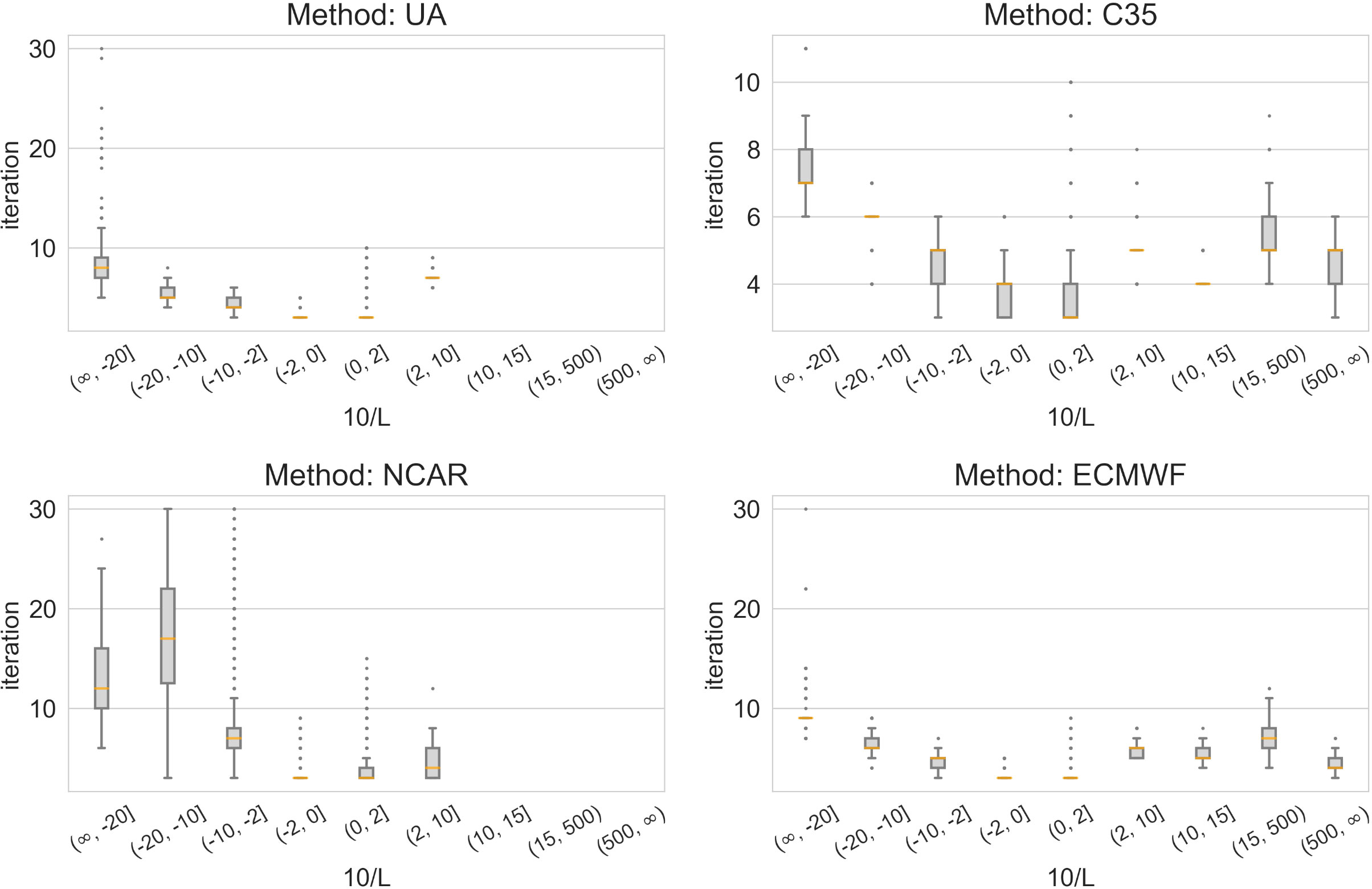
Figure 6 Boxplots of the number of iterations needed for convergence (in AirSeaFluxCode) relative to various stability ranges (10/L_tsrv), showing the median (orange line), the inter-quartile range (25–75%, box), the outer range (whiskers, < 25% and > 75% respectively). Outliers (0.7% of data) are shown as grey dots. The four parameterizations examined in Section 3.1 are shown. For UA, C35 and ECMWF gustiness is switched on selecting option 1 with β_conv=1.2, z_i=600 m and u_gmin=0.01 ms^–1.

Table S25 summarizes the “failure” rates for all tests. It can be seen that using a constant rather than a function for the acceleration of gravity, c_p, L_v, ρ₀ and Г has no impact on the failure rate, and neither does the method of calculating e_s. Completely neglecting the 2% salt reduction of q₀ has little or no impact in the failure rates of most parameterizations, but increases the failure rate in LP82 and NCAR (although it should be noted that all of the 10 parameterizations do include the 2% reduction term).

The choice of method for Monin-Obukhov length has a mixed impact that differs according to the parameterization chosen: by far the biggest impact is the reduction in failure rates for LP82 and NCAR (falling from 0.99% to 0.03%, and from 1.66% to 0.18% respectively) when the L_Rb method is chosen. The high failure rates in LP82 and NCAR when using L_tsrv occurred under moderate to high wind speeds in near-neutral stability conditions (Figure S4) and were due to the use of distinct values for the heat transfer coefficients under stable and unstable conditions. Under near-neutral conditions the iteration may oscillate between stable and unstable conditions and coefficients, producing flux results that differ by more than the tolerance limits and hence preventing the iteration from converging. In contrast, the failure rate almost doubles for UA when the L_Rb method is applied with the additional failed data occurring under stable conditions.

If we exclude the results for LP82 and NCAR when the L_tsrv method is used, then Figure S4 shows that failures always occur under low wind speeds (less than about 5 ms^–1) with atmospheric conditions that are very stable or very unstable. In the default versions of the algorithms (i.e. using L_tsrv), NCAR has the largest failure rates (1.66%), followed by LP82 (0.99%), YT96 (0.58%), UA (0.26%), S80 (0.09%), ECMWF (0.08%), Beljaars (0.08%), S88 (0.07%), and C30 and C35 (both 0.04%).

Applying the gustiness term and using the default (option 1) for removing the effects of gustiness from τ and the wind speed parameters slightly decreases the failure rate for most parameterizations. The exceptions are S88 and LP82 where using option 1 increases their failure rate by generating negative values of u_10n due to over-correction at very low wind speeds. The user should be careful when choosing a value for u_gmin since increasing the default value (0.01 ms^–1) increases the failure rate (Table S24).

The application of the cool skin/warm layer adjustment has a direct impact on the stability through the adjustment of ΔT at every iteration step; in near neutral conditions the adjustment can lead to changes between stable/unstable conditions. Applying the cool skin adjustment (only) following Fairall et al. (1996a); Edson et al. (2013) has very little impact on the failure rates for most of the parameterizations, with only marginal increases in failure for S80, S88 and C35. However, the increase in failure rates is larger for LP82 and NCAR which are more sensitive to shifts between un/stable conditions. When the warm layer adjustment is also applied, the increase in failure rates is removed. The application of the cool skin adjustment (only) following ECMWF (2019) has a similar impact on failure rates compared to applying the default (C35, Fairall et al., 1996a; Edson et al., 2013): failure rates are marginally higher for some parameterizations and marginally lower for others.

3.3 Summary of results

Section 3.2 describes in detail various comparisons and tests of AirSeaFluxCode using the ERA5 test dataset which contained data spanning a very wide range of wind speed and atmospheric stability conditions. The results are summarized here.

Section 3.2.1 examined the effect of approximating some thermodynamic variables as constant values rather than using their functional dependencies. The choice of the form of Г had no impact (Table S12). For acceleration due to gravity, c_p and L_v, using a constant rather than the more accurate functional form had limited impact but the functional form is simple to calculate and should be used. In contrast, using a constant density of air had serious impacts across all wind speeds and stabilities, with systematic increase of heat loss in the tropics of order 10 Wm^–2, and systematic decrease of heat loss in higher latitudes also of order 10 Wm^–2. The constant approximation for air density should never be used.

Section 3.2.2 tested the default formulation for determining the Monin-Obukhov length (L_tsrv) against the alternative (L_Rb) and found differences in the lhf output that were significant in a few cases when wind speed was low and stability extreme. The differences in the resulting 10/L estimates are largest when |10/L| is large (Figure S3) i.e. when the stability functions show the most variation between parameterizations (Figure 2). L_tsrv is the formulation normally favoured by algorithm developers. Use of L_Rb enables data in near neutral, high wind speed conditions, to converge when using the LP82 and NCAR parameterizations: in these conditions L_tsrv oscillates in sign throughout the iteration, causing selection of different values for the heat transfer coefficients and hence large changes in the heat fluxes between iterations which leads to a failure to converge.

Section 3.2.3 examined various formulations for saturation vapour pressure functions (e_s). No significant differences were found, but in the mean there was a systematic change in lhf of about 0.2 Wm^–2.

Section 3.2.4 examined the impact of the 2% reduction in q to account for the salinity of sea water. If neglected entirely this would have a dramatic impact on the lhf, but that is no longer common practice. However, there is uncertainty in the correct percentage to use: if the 2% term is replaced by 1.8% or 2.2% then the lhf begins to see significant changes; if replaced by 1.6% or 2.4% significant changes occur in about 50% of the lhf results.

Section 3.2.5 examined the impact of applying the cool skin and warm layer adjustments. It was noted that some parameterizations were developed based on bulk sea temperature measurements made at depths of about 1 m or more, whereas others were developed based on “skin” temperature data (either from radiometric measurements or modelled). If the input temperatures are bulk measurements then either (a) a parameterization based on such data should be used or (b) both the cool skin and the warm layer adjustments should be applied if using a parameterization that was developed using skin temperature. These adjustments have a dramatic effect on the heat fluxes: for the shf about 50% of data show significant changes; for the lhf more than 47% show significant changes and a further ~20% or more show major changes. The parameterization should therefore be chosen carefully with regard to the available input data.

Section 3.2.6 examined the use of the gustiness term (Equation 9). This term is included in some parameterizations in order to produce non-zero heat fluxes under very low wind speed, convective conditions. However, its use impacts all the fluxes across all wind speeds. For this reason the effects of the gustiness term are usually removed from τ (and also from u_10n as the default in AirSeaFluxCode and all developer codes except ECMWF) after the iteration has converged using a gustiness factor, but some significant differences still remain. As expected, the application of the gustiness term increases the heat fluxes but the impacts are seen at moderate and high winds as well as under low winds speeds. For the shf significant differences are seen for wind speeds up to 20 ms^–1, with an increased heat loss from the ocean of about 0.15 Wm^–2 on average. For lhf, significant differences are also seen across all wind speeds, with a mean increase of heat loss of about 1 Wm^–2. At low wind speeds the lhf sees major differences, with increased heat loss of nearly 3 Wm^–2 in the 5^th percentile, and maximum changes of between 10 and 30 Wm^–2 depending on the parameterization. As expected, applying the gustiness term slightly decreased “failure” rates with the exception of S88 and LP82 where the rates increased slightly (using the default option 1).

In Section 3.2.7, Table S25 combined results from the above tests to examine the “failure” rates in AirSeaFluxCode where “failure” is defined as; non-physical u_10n, T_10n or q_10n results; lack of convergence after 30 iterations. Across all comparisons and tests, the rates are either small (less than about 0.5%) or, in the case of the LP82 and NCAR parameterizations, can be reduced to < 0.5% by choosing L_Rb (see Section 3.2.7). In general, data fail under low wind speeds and large |10/L|. Failure rates are increased by any discontinuities in the algorithm, e.g. different transfer coefficients for un/stable conditions.

4 Discussion

AirSeaFluxCode is an open source software package that calculates the turbulent air-sea fluxes of momentum, sensible heat and latent heat from mean meteorological and sea surface parameters. It also adjusts the mean meteorological parameters to a user-defined output height and also outputs 10 m neutral values. To date, it includes ten different existing bulk formulae parameterizations (Table 1).

The choice of parameterization has by far the biggest impact on the calculated fluxes due to the wide range of values assigned to the transfer coefficients and/or roughness lengths. AirSeaFluxCode allows these differences to be easily examined without the need to implement the various developer codes or write new code for parameterizations that lack publicly available code.

AirSeaFluxCode was tested against the available code provided by the developers of four of the ten bulk parameterizations. A few significant or major differences were found in the flux results in the comparison with the developer code for ECMWF and NCAR. In general these differences were due to different choices made in the calculation of basic functions (e.g. ρ₀, c_p), limits applied to basic parameters (e.g. u_10n, z_0m) and the assumption of convergence after just 5 iterations in the developer code: we demonstrated that up to 30 iterations were required for convergence under very stable or unstable atmospheric conditions. In contrast, for UA and C35 there were no significant differences in the flux results. In general the agreement between AirSeaFluxCode and the developer codes was excellent which provides confidence that AirSeaFluxCode functions as expected and is robust.

The flux results from any individual parameterization can be significantly affected by the choices made in order to implement it. AirSeaFluxCode includes a wide range of implementation options (e.g. method of calculating the Monin-Obukhov length, gustiness, cool skin etc.) so that the sensitivity of the fluxes to these options can also be explored. In this paper we have used AirSeaFluxCode to quantify the impact of some of these options on the fluxes, and on the height- and stability-adjusted meteorological parameters u_10n, T_10n and q_10n.

As a result of the sensitivity tests made in this paper we can make the following recommendations:

The functional forms of air density, latent heat of evaporation and specific heat capacity (see Table S1) should be used, since approximating these variables by constant values leads to significant and/or systematic errors.

The user should choose parameterizations and/or implementation options appropriate to their input data, otherwise there may be unintended, significant impacts on the calculated fluxes. Some parameterizations were developed using particular input data, e.g. wind speeds relative to surface currents (rather than earth-relative), or a sea surface “skin” temperature rather than a bulk temperature. If a parameterization requires particular variables but instead the user substitutes an estimate, or an inappropriate variable (such as bulk temperature instead of skin temperature), then the errors and uncertainty in the calculated fluxes etc. will be substantially increased.

The limit on the maximum number of iterations allowed should be chosen with care. For typical open ocean conditions the calculations rapidly converge but under low wind speeds when conditions are either very unstable or very stable, the calculations may require many iterations to converge. Under extreme conditions convergence may not be possible since the theory underpinning the calculations is at, or even beyond, the limits of its applicability: all ten parameterizations failed to converge for a very small fraction of data even after 30 iterations. Values calculated under such conditions will be highly uncertain, but if a zero failure rate is required then the user has the option to output all data, with flags to indicate where data has not converged or where the results may be non-physical.

Discontinuities in the underlying functions should be avoided. For example, the use by LP82 and NCAR of distinct values for the heat transfer coefficients in stable and unstable conditions meant that near-neutral data did not converge when used with the default L_tsrv method of calculating the Monin-Obukhov length. Such near-neutral data usually converge very quickly but in these two parameterizations the iteration oscillated between two values with differences that exceeded the tight tolerance criteria imposed in the test for convergence.

The reduction factor for saturation vapor pressure due to salinity needs to be better constrained and its uncertainty established. It is important to include the effects of salinity when calculating the saturation vapor pressure. The reduction value typically used is 2.0%, but an uncertainty of just 0.2 (i.e. a value of either 1.8 or 2.2%) has a significant impact on the latent heat fluxes.

The impact of using ad hoc constraints as often used in the original developer code (e.g. setting a lower limit on wind speed or constraining the value of the Monin-Obukhov length etc), should be carefully evaluated. Such constraints may enable an algorithm to avoid producing un-physical outputs in extreme conditions, but can have significant impacts on the resulting fluxes and height- and stability adjusted meteorological parameters.

The impact of including the effects of convective gustiness in a parameterization, should be carefully evaluated. Including gustiness is usually justified in terms of producing non-zero heat fluxes at low wind speeds, but it significantly increases those fluxes under moderate and high wind speeds as well. The gustiness term also produces significant increases in the momentum flux and u_10n at all wind speeds: various approaches are taken to removing (or reducing) these effects from those output parameters but significant differences remain in the momentum flux at high wind speeds for most parameterizations. In addition, when the effects of gustiness are removed from the output TSF some other parameters become inconsistent with each other. In particular, the values output for u_* retain the impacts of the gustiness term, and are inconsistent with the output momentum flux. Similarly, if the effects of gustiness were removed from u_* (by applying the gust factor), it would no longer be consistent with the output drag coefficients. The application of a gustiness parameterization is often thought to improve convergence of the iterative calculation but the improvement is very small in most parameterization and for others the convergence rate actually decreases slightly.

Our code was designed to allow easy exploration of the different bulk formulae parameterizations and the wide range of implementation options. A high standard was set for the output data in that strict tolerance criteria were set when testing if the iteration had converged. This means that the code may be more computationally demanding than some applications require. To some extent this can be addressed by the user by relaxing the tolerance criteria, or reducing the maximum number of iterations allowed, but this would have to be weighed against the increased uncertainty in the results. Similarly, the default setting in our code is to set data that have not converged, or have produced non-physical values, to absent. Again, if this is unsuited to a particular application the user can output all data, flagged as appropriate.

We intend to regularly expand and update the code. Our priorities will be: to include new parameterizations that are published; to extend the calculations to include parameterizations that incorporate the effects of sea state; and, to develop and incorporate uncertainty estimates to accompany the calculations. We welcome collaboration on the development of the software package, as well as any bug reports, corrections or comments.

Data availability statement

The original contributions presented in the study are included in the article/Supplementary Material. Further inquiries can be directed to the corresponding author.

Author contributions

SB and RC wrote the Python code, substantially developing earlier FORTRAN software by EK and DB and R software by EK and RC. SB wrote the paper. EK and MY contributed to the analysis and interpretation of the results. All authors contributed to manuscript revision, read, and approved the submitted version.

Funding

This work is supported by the Natural Environment Research Council grants ORCHESTRA, (NE/N018095/1), ENCORE (NE/V013254/1) and CLASS (NE/R015953/1).

Acknowledgments

Hersbach et al. (2018) was downloaded from the Copernicus Climate Change Service (C3S) Climate Data Store. The results contain modified Copernicus Climate Change Service information 2020. Neither the European Commission nor ECMWF is responsible for anyuse that may be made of the Copernicus information or data it contains. The results contain data from Smith et al. (2019). We would like to thank: Dr Thomas Cropper for his useful comments and input; Dr Chris Banks for testing the code, Dr Peter K Taylor for his contribution to the original FORTRAN software.

Conflict of interest

The authors declare that the research was conducted in the absence of any commercial or financial relationships that could be construed as a potential conflict of interest.

Publisher’s note

All claims expressed in this article are solely those of the authors and do not necessarily represent those of their affiliated organizations, or those of the publisher, the editors and the reviewers. Any product that may be evaluated in this article, or claim that may be made by its manufacturer, is not guaranteed or endorsed by the publisher.

Supplementary material

The Supplementary Material for this article can be found online at: https://www.frontiersin.org/articles/10.3389/fmars.2022.1049168/full#supplementary-material

References

Alappattu D. P., Wang Q., Yamaguchi R., Lind R. J., Reynolds M., Christman A. J. (2017). Warm layer and cool skin corrections for bulk water temperature measurements for air-sea interaction studies. J. Geophysical Research: Oceans 122, 6470–6481. doi: 10.1002/2017JC0126

CrossRef Full Text | Google Scholar

Beljaars A. C. M. (1995a). “The impact of some aspects of the boundary layer scheme in the ECMWF model,” in Proc. seminar on parameterization of Sub-grid scale physical processes, reading (United Kingdom: ECMWF).

Google Scholar

Beljaars A. C. M. (1995b). The parameterization of surface fluxes in large scale models under free convection. Quart. J. R. Meteor. Soc 121, 255–270. doi: 10.1002/qj.49712152203

CrossRef Full Text | Google Scholar

Beljaars A. C. M., Holtslag A. A. M. (1991). Flux parameterization over land surfaces for atmospheric models. J. Appl. Meteorology 30, 327–341. doi: 10.1175/1520-0450(1991)030<0327:fpolsf>2.0.co;2

CrossRef Full Text | Google Scholar

Bentamy A., Piollè J. F., Grouazel A., Danielsone R., Gulev S., Paul F., et al. (2017). Review and assessment of latent and sensible heat flux accuracy over the global oceans. Remote Sens. Environ. 201, 196–218. doi: 10.1016/j.rse.2017.08.016

CrossRef Full Text | Google Scholar

Berry D. I., Kent E. C. (2009). A new air–sea interaction gridded dataset from ICOADS with uncertainty estimates. Bull. Am. Meteorological Soc. 90, 645–656. doi: 10.1175/2008bams2639.1

CrossRef Full Text | Google Scholar

Bosilovich M. G., Robertson F. R., Chen J. (2011). Global energy and water budgets in MERRA. J. Climate 24, 5721–5739. doi: 10.1175/2011jcli4175.1

CrossRef Full Text | Google Scholar

Bourassa M. A., Gille S. T., Bitz C., Carlson D., Clayson C. A., Cerovecki I. (2013). High-latitude ocean and sea ice surface fluxes: challenges for climate research. Bull. Am. Met. Soc 94, 403–423. doi: 10.1175/bams-d-11-00244

CrossRef Full Text | Google Scholar

Bradley F., Fairall C. (2006). A guide to making climate quality meteorological and flux measurement at sea. NOAA Tech. Memorandum OAR PSD 311, 311. https:///repository.library.noaa.gov/view/noaa/17408

Google Scholar

Brodeau L., Barnier B., Gulev S., Woods C. (2017). Climatologically significant effects of some approximations in the bulk parameterizations of turbulent air-sea fluxes. J. Phys. Oceanogr. 47, 5–28. doi: 10.1175/JPO-D-16-0169.1

CrossRef Full Text | Google Scholar

Brunke M. A., Fairall C. W., Zeng X., Eymard L., Curry J. A. (2003). Which bulk aerodynamic algorithms are least problematic in computing ocean surface turbulent fluxes? J. Climate 16:619–635. doi: 10.1029/2019GL084156

CrossRef Full Text | Google Scholar

Buck A. L. (1981). New equations for computing vapor pressure and enhancement factor. J. Appl. Meteorol. 20, 1527–1532. doi: 10.1175/1520-0450(1981)020<1527:NEFCVP>2.0.CO;2

CrossRef Full Text | Google Scholar

Buck A. L. (2012). Model CR-1A hygrometer with autofill operating manual (Boulder, CO 80308: Buck Research Instruments, LLC). Available at: http://www.hygrometers.com/wp-content/uploads/CR-1A-users-manual-2009-12.pdf.

Google Scholar

Busch N. (1973). “On the mechanics of atmospheric turbulence,” in Workshop on micrometeorology (Boston: American Meteorological Society), 1–65.

Google Scholar

Cronin M. F., Fairall C. W., McPhaden M. J. (2006). An assessment of buoy-derived and numerical weather prediction surface heat fluxes in the tropical pacific. J. Geophysical Research: Oceans 111:1–8. doi: 10.1029/2005JC003324

CrossRef Full Text | Google Scholar

Cronin M. F., Gentemann C. L., Edson J., Ueki I., Bourassa M., Brown S., et al. (2019). Air-sea fluxes with a focus on heat and momentum. Front. Mar. Sci. 6. doi: 10.3389/fmars.2019.00430

CrossRef Full Text | Google Scholar

Dee D. P., Uppala S. M., Simmons A. J., Berrisford P., Poli P., Kobayashi S., et al. (2011). The era-interim reanalysis: configuration and performance of the data assimilation system. Quartely J. R. Meteorological Soc. 137, 553–597. doi: 10.1002/qj.828

CrossRef Full Text | Google Scholar

Donlon C. J., Minnett P. J., Gentemann C., Nightingale T. J., Barton I. J., Ward B., et al. (2002). Toward improved validation of satellite sea surface skin temperature measurements for climate research. J. Climate 15, 353–369. doi: 10.1175/1520-0442(2002)015<0353:tivoss>2.0.co;2

CrossRef Full Text | Google Scholar

Dyer A. J. (1974). A review of flux-profile relationships. Boundary-Layer Meteorology 7, 363–372. doi: 10.1007/BF00240838

CrossRef Full Text | Google Scholar

ECMWF (2014). “Part IV: Physical processes,” in Turbulent transport and interactions with the surface. IFS documentation Cy40r1. operational implementation 22 November 2013 (Reading, RG2 9AX, England: ECMWF), 35–37. Available at: https://www.ecmwf.int/sites/default/files/elibrary/2014/9204-part-iv-physical-processes.pdf.

Google Scholar

ECMWF (2019). “Part IV: Physical processes,” in Turbulent transport and interactions with the surface. IFS documentation CY46R1 (Reading, RG2 9AX, England: ECMWF), 33–58. Available at: https://www.ecmwf.int/node/19308.

Google Scholar

Edson J. B., Jampana V., Weller R. A., Bigorre S. P., Plueddemann A. J., Fairall C. W., et al. (2013). On the exchange of momentum over the open ocean. J. Phys. Oceanography 43:1589–1610. doi: 10.1175/JPO-D-12-0173.1

CrossRef Full Text | Google Scholar

Fairall C. W., Bradley E. F., Godfrey J. S., Wick G. A., Edson J. B., Young G. S. (1996a). Cool-skin and warm-layer effects on sea surface temperature. J. Geophysical Res. 101, 1295–1308. doi: 10.1029/95JC03190

CrossRef Full Text | Google Scholar

Fairall C. W., Bradley E. F., Hare J. E., Grachev A. A., Edson J. B. (2003). Bulk parameterization of air-sea fluxes: updates and verification for the coare algorithm. J. Climate 16, 571–591. doi: 10.1175/1520-0442(2003)016<0571:BPOASF>2.0.CO;2

CrossRef Full Text | Google Scholar

Fairall C. W., Bradley E. F., Rogers D. P., Edson J. B., Young G. S. (1996b). Bulk parameterization of air-sea fluxes for tropical ocean global atmosphere coupled-ocean atmosphere response experiment. J. Geophysical Res. 101, 3747–3764. doi: 10.1029/95JC03205

CrossRef Full Text | Google Scholar

Grachev A. A., Fairall C. W. (1997). Dependence of the monin–obukhov stability parameter on the bulk richardson number over the ocean. J. Appl. Meteorology 36, 406–414. doi: 10.1175/1520-0450(1997)036<0406:DOTMOS>2.0.CO;2

CrossRef Full Text | Google Scholar

Grachev A. A., Fairall C. W., Bradley E. F. (2000). Convective profile constants revisited. Boundary-Layer Meteorology 94, 495–515. doi: 10.1023/a:1002452529672

CrossRef Full Text | Google Scholar

Gulev S. K. (1994). Influence of space-time averaging on the ocean-atmosphere exchange estimates in the north atlantic midlatitudes. J. Phys. Oceanography 24, 1236–1255. doi: 10.1175/1520-0485(1994)024<1236:IOSTAO>2.0.CO;2

CrossRef Full Text | Google Scholar

Hersbach H., Bell B., Berrisford P., Biavati G., Horányi A., noz Sabater J. M., et al. (2018) Era5 hourly data on single levels from 1979 to present (Copernicus Climate Change Service (C3S) Climate Data Store (CDS) (Accessed 14-AUG-2020).

Google Scholar

Hersbach H., Bell B., Berrisford P., Hirahara S., Horányi A., Muñoz-Sabater J., et al. (2020). The ERA5 global reanalysis. Q. J. R. Meteorological Soc. 146, 1999–2049. doi: 10.1002/qj.3803

CrossRef Full Text | Google Scholar

Kobayashi S., OTA Y., HARADA Y., EBITA A., MORIYA M., ONODA H., et al. (2015). The JRA-55 reanalysis: General specifications and basic characteristics. J. Meteorological Soc. Japan. Ser. II 93, 5–48. doi: 10.2151/jmsj.2015-001

CrossRef Full Text | Google Scholar

Kraus E. B., Businger J. A. (1995). Atmosphere-ocean interaction (New York: Oxford University Press). doi: 10.1093/oso/9780195066180.001.0001

CrossRef Full Text | Google Scholar

Large W. G. (1979). The turbulent fluxes of momentum and sensible heat over the open Sea during moderate to strong winds (Vancouver, BC, Canada: Ph.D. thesis, University of British Columbia, Vancouver Institute of Oceanography).

Google Scholar

Large W. G., Danabasoglu G., Doney S. C., McWilliams J. C. (1997). Sensitivity to surface forcing and boundary layer mixing in a global ocean model. J. Phys. Oceanography 27, 2418–2447. doi: 10.1175/1520-0485(1997)027,2418:STSFAB.2.0.CO;2

CrossRef Full Text | Google Scholar

Large W. G., Pond S. (1981). Open ocean momentum flux measurements in moderate to strong winds. J. Phys. Oceanography 11, 324–336. doi: 10.1175/1520-0485(1981)011<0324:oomfmi>2.0.co;2

CrossRef Full Text | Google Scholar

Large W. G., Pond S. (1982). Sensible and latent heat flux measurements over the ocean. J. Phys. Oceanography 12, 464–482. doi: 10.1175/1520-0485(1982)012<0464:SALHFM>2.0.CO;2

CrossRef Full Text | Google Scholar

Large W. G., Yeager S. (2004). Diurnal to decadal global forcing for ocean and sea-ice models: The data sets and flux climatologies. Univ. Corporation Atmospheric Res. doi: 10.5065/D6KK98Q6

CrossRef Full Text | Google Scholar

Large W. G., Yeager S. (2009). The global climatology of an interannually varying air–sea flux data set. Climate Dyn. 33, 341–364. doi: 10.1007/s00382-008-0441-3

CrossRef Full Text | Google Scholar

Ledvina D. V., Young G. S., Miller R. A., Fairall C. W. (1993). The effect of averaging on bulk estimates of heat and momentum fluxes for the tropical western pacific ocean. J. Geophysical Res. 98:20211–20217. doi: 10.1029/93JC01856

CrossRef Full Text | Google Scholar

MATLAB (2018) (Natick, Massachusetts). 9.7.0.1190202 (R2019b).

Google Scholar

Powell M. D., Vickery P. J., Reinhold T. A. (2003). Reduced drag coefficient for high wind speeds in tropical cyclones. Nature 422, 279–283. doi: 10.1038/nature01481

PubMed Abstract | CrossRef Full Text | Google Scholar

Sanchez-Franks A., Kent E. C., Matthews A. J., Webber B. G. M., Peatman S. C., Vinayachandran P. N. (2018). Intraseasonal variability of air–sea fluxes over the bay of Bengal during the southwest monsoon. J. Climate 31, 7087–7109. doi: 10.1175/jcli-d-17-0652.1

CrossRef Full Text | Google Scholar

Smith S. D. (1980). Wind stress and heat flux over the ocean in gale force winds. J. Phys. Oceanography 10, 709–726. doi: 10.1175/1520-0485(1980)010<0709:WSAHFO>2.0.CO;2

CrossRef Full Text | Google Scholar

Smith S. D. (1988). Coefficients for sea surface wind stress, heat flux, and wind profiles as a function of wind speed and temperature. J. Geophysical Res. 93, 15467–15472. doi: 10.1029/JC093iC12p15467

CrossRef Full Text | Google Scholar

Smith S. R., Briggs K., Bourassa M. A., Elya J., Paver C. R. (2018). Shipboard automated meteorological and oceanographic system data archive: 2005–2017. Geosci. Data J. 5, 73–86. doi: 10.1002/gdj3.59

CrossRef Full Text | Google Scholar

Smith S. R., Rolph J. J., Briggs K., Bourassa M. A. (2019) Quality controlled shipboard automated meteorological and oceanographic system (SAMOS) data (Tallahassee, FL, USA: Center for Ocean-Atmospheric Prediction Studies, The Florida State University). Available at: http://samos.coaps.fsu.edu (Accessed 15 11 2019).

Google Scholar

Stull R. B. (1988). An introduction to boundary layer meteorology (Dordrecht, The Netherlands: Springer Netherlands). doi: 10.1007/978-94-009-3027-8

CrossRef Full Text | Google Scholar

Taylor P. K. (2000). Intercomparison and validation of ocean–atmosphere energy flux fields. final report of the joint WCRP/SCOR working group on air–Sea fluxes (SCOR working group 110). WCRP report 112, WMO/TD-1036 (Geneva: World Meteorological Organization, World Climate Research Programme).

Google Scholar

Van Rossum G., Drake F. L. (2009). Python 3 reference manual (Scotts Valley, CA: CreateSpace).

Google Scholar

Vehkamäki H., Kulmala M., Napari I., Lehtinen K. E. J., Timmreck C., Noppel M., et al. (2002). An improved parameterization for sulfuric acid–water nucleation rates for tropospheric and stratospheric conditions. J. Geophys. Res. 107, 4622. doi: 10.1029/2002JD002184

CrossRef Full Text | Google Scholar

WMO (2018). “Guide to meteorological instruments and methods of observation,” in Annex 4.B. formulae for the computation of measures of humidity. WMO-no. 8 2018. 188 (Geneva: WMO).

Google Scholar

Yelland M., Moat B. I., Taylor P. K., Pascal R. W., Hutchings J., Cornell V. C. (1998). Wind stress measurements from the open ocean corrected for airflow distortion by the ship. J. Phys. Oceanography 28, 1511–1526. doi: 10.1175/1520-0485(1998)028<1511:WSMFTO>2.0.CO;2

CrossRef Full Text | Google Scholar

Yelland M., Taylor P. K. (1996). Wind stress measurements from the open ocean. J. Phys. Oceanography 26, 541–558. doi: 10.1175/1520-0485(1996)026<0541:WSMFTO>2.0.CO;2

CrossRef Full Text | Google Scholar

Yu L. (2019). Global air–sea fluxes of heat, fresh water, and momentum: Energy budget closure and unanswered questions. Annu. Rev. Mar. Sci. 11, 227–248. doi: 10.1146/annurev-marine-010816-060704

CrossRef Full Text | Google Scholar

Zeng X., Beljaars A. (2005). A prognostic scheme of sea surface skin temperature for modeling and data assimilation. Geophys. Res. Lett. 32:1–4. doi: 10.1029/2005gl023030

CrossRef Full Text | Google Scholar

Zeng X., Zhao M., Dickinson R. (1998). Intercomparison of bulk aerodynamic algorithms for the computation of sea surface fluxes using TOGA COARE and TAO data. J. Climate 11, 2628–2644. doi: 10.1175/1520-0442(1998)011<2628:IOBAAF>2.0.CO;2

CrossRef Full Text | Google Scholar