Simulation of high-frequency dissolved oxygen dynamics in a shallow estuary, the Corsica River, Chesapeake Bay

1 Introduction

Eutrophication and hypoxia caused by anthropogenic nutrient loading to coastal and estuarine systems is an ever-growing environmental challenge in the 21^st century (Diaz and Rosenberg, 2008; Howarth et al., 2011; Rabalais et al., 2014; Hale et al., 2016). Chesapeake Bay, the largest estuary in the U.S. and the third largest worldwide, continues to experience hypoxia during summer (Boynton, 1997; Murphy et al., 2011; Scavia et al., 2021). Even though hypoxia has been observed since the early 1900s (Sale and Skinner, 1917; Newcombe and Horne, 1938), hypoxic water volume tripled from 1950 to 2000 (Hagy et al., 2004). Efforts have been made to restore the Bay through management and nutrient load reductions (U.S. EPA, 2010; Linker et al., 2013; Shenk and Linker, 2013; U.S. EPA, 2021), and these reductions have resulted in modest reductions in hypoxia (Testa et al., 2018; Ni et al., 2020; Frankel, 2021).

In contrast to the focus on seasonal, deep-water hypoxia in Chesapeake Bay and other large coastal systems (Scavia et al., 2003; Carstensen et al., 2014), less attention has been given to high-frequency hypoxia in shallow, nearshore areas. While these hypoxia events may be short-lived, they often lead to indirect effects, such as avoidance of nursery habitats (Brady and Targett, 2010; Brady and Targett, 2013), and direct effects on growth and mortality (Stierhoff et al., 2009). An array of physical dynamics, such as tidal mixing and advection, waves, sea level rise, river flow, sediment and nutrient loads interact to generate a complex water quality regime that differ in the timescale of responses relative to deeper waters (McGlathery et al., 2013; Xiao et al., 2021). Feedbacks and interactions between biotic and abiotic processes can also lead to nonlinear response in water quality to environmental forcing (Su et al., 2022). Technical advancement in both continuous monitoring sensors and unstructured grid models capable of resolving shallow water features can help to better understand the physical and biological dynamics that underpin the variability in water quality in coastal shallow systems. A significant number of continuous water quality electronic sensors have been deployed in the shallow regions in Chesapeake Bay, which provide unprecedented continuous high-frequency monitoring data (CONMON). The sensor data have revealed high-frequency variability in water quality in shallow systems with large amplitude variations within hours (Shen et al., 2008; Graziano and Jones, 2017; Duvall et al., 2022). The high-frequency variability represents a fundamental challenge to our concept and understanding of ecosystem function and water quality dynamics, which were previously based on an extrapolation from deep water Bay studies.

The Corsica River, a sub-tributary in Chesapeake Bay (Figure 1) is an excellent case study that demonstrates the challenges in characterizing and managing shallow estuarine water quality (U.S. EPA, 2013). The major land uses in its watershed are agriculture (64%), woodland (28%) and developed areas. The Corsica River provides vital habitats for numerous species as well as recreational uses. However, high nutrient concentrations (above algal nutrient-limitation levels), high algal abundance (measured by chlorophyll-a concentrations), and low DO events occur in the summer and recur each year (Boynton et al., 2009). It is classified as impaired by the Maryland Department of Natural Resources. Fish-kill events due to hypoxic conditions have also been reported U.S. EPA (2013). To investigate the ecosystem function and water quality dynamics in the Corsica River, continuous monitoring data (every 15 minutes) have been collected at multiple locations. In this study, a state-of-art model, Semi-implicit Cross-scale Hydroscience Integrated System Model (SCHISM), coupled with the Army Corps of Engineers Integrated Compartment water quality model (ICM), was implemented in the Corsica River estuary, USA with a high-resolution unstructured grid (Figure 1). The objective of the project is to determine the capacity of this modeling system to simulate observed high-frequency water quality variability in the Corsica River and to shed new light on ecosystem function and water quality dynamics in the shallow systems, with an emphasis on understanding the factors controlling high-frequency variability in dissolved oxygen.

FIGURE 1

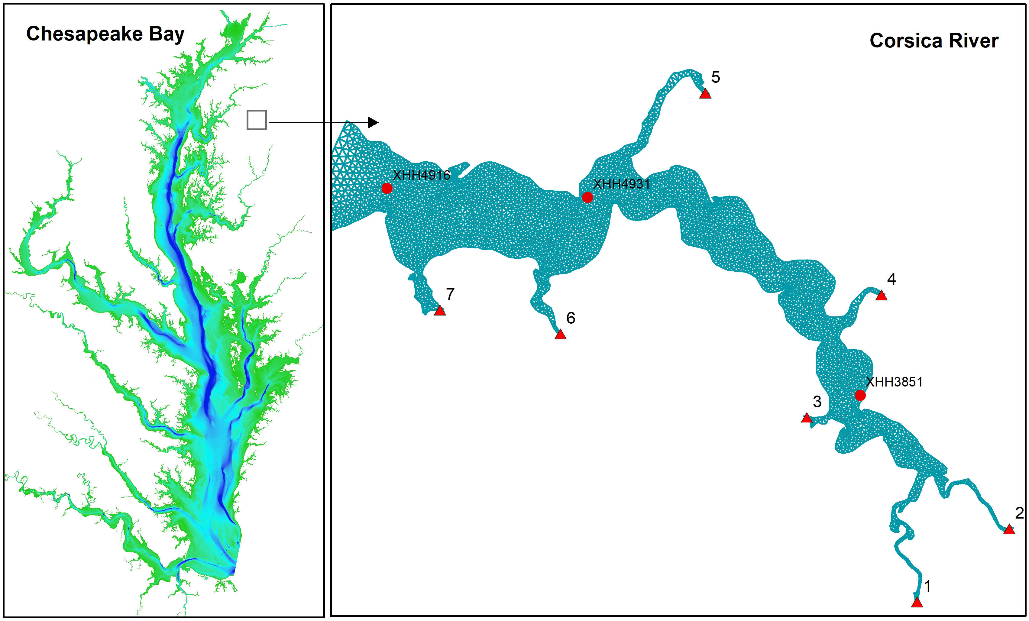
Figure 1 Geographic location of the simulation domain and grid. Background color of the left panel is the bathymetry ranging up to 40 m (blue). Red triangles on the right panel are the seven freshwater discharge locations from the watershed. Red dots are the four stations with both cruise-based sample data and sensor-based continuous monitoring data.

2 Methods

2.1 Models

SCHISM and ICM have been described in detail in the literature (available at https://www.schism.wiki) and only a brief description relevant to the interpretation of the simulation results is given here. SCHISM employs an unstructured grid with a highly efficient semi-implicit finite-element Eulerian-Lagrangian algorithm to solve the Navier-Stokes equations and transport for the physical fields (Zhang et al., 2016). In the version used here, ICM (Cerco and Cole, 1994; Cerco and Noel, 2004; Cai et al., 2020; Cai et al., 2021) consists of 21 state variables including multiple species of inorganic nitrogen and phosphorus, multiple forms of dissolved and particulate organic nitrogen, organic phosphorus, and organic carbon, three groups of phytoplankton (Diatoms, Green Algae and Cyanobacteria) as carbon, chemical oxygen demand (COD) and dissolved oxygen (DO). The governing equation of phytoplankton (B) is written as:

$\begin{array}{ll}\frac{\partial B}{\partial t}=\left(\mu -{\alpha }_m\right)·B-{\alpha }_P·B +\nabla ·\left(uB\right)+\left(D\nabla B\right)& \text{.(1),}\end{array}$

where µ is phytoplankton growth rate, α_m is the respiration coefficient, α_p is the coefficient for predation loss and the last two terms are physical advection and turbulent diffusion, respectively. The phytoplankton growth rate (μ) is determined by temperature, light limitation (Jassby and Platt, 1976) and nutrient limitation, which is parameterized using the Michaelis-Menten function:

$\begin{array}{ll}\mu ={\mu }_{max}{e}^{-K_{T\left(1,2\right)}{\left(T-T_o\right)}^2}·\frac{I}{\sqrt{I^2+K_I^2}}·\min \left(\frac{N}{N+K_N},\frac{P}{P+K_P}\right)& (2)\end{array}$

where µ_max is the maximum growth rate, T_O is the optimal temperature where phytoplanoton growth rate reaches its maximum, K_T(1,2) is the exponential coefficient determining the temeprature control on phytoplankton growth with K_T(1) applied to temperature below the the optimal temperature and K_T(2) for temperature above the optimal tempetaure, I is the photosynthetically active radiation (PAR), K_I is the parameter defining the growth-radiation curve, N and P are nitrogen and phosphorous concentration, and K_N and K_P are the corresponding half-saturation coefficients. DO is a crucial state variable in the ICM water quality model. DO is determined by photosynthetic production, consumption by phytoplankton respiration, DOC remineralization, nitrification, the oxidation of reduced solutes (chemical oxygen demand, or COD), aereation at the the sea surface, and sediment and tidal wetland oxygen demand at the bottom:

$\begin{array}{ll}\frac{\partial DO}{\partial t}=a_{OC}\left[\left(1.3-0.3p_{NH}\right)·\mu -{\alpha }_m\right]·B-a_{ON}·NT-{\alpha }_{DOC}·a_{OC}·\frac{DO}{k_{OC}+DO}·DOC& (\mathrm{})\end{array}$

$\begin{array}{ll}-{\alpha }_{COD·}\frac{DO}{k_{COD}+DO}·COD+\frac{{\alpha }_{air}}{D{Z}_S}\left(DOs-DO\right)-\frac{SOD}{D{Z}_R}-f\left(T\right)\frac{{\alpha }_W{A}_W}{D{Z}_R}& (3)\end{array}$

where a_OC is the O:C ratio in phytoplankton, p_NH is the ammonium preference for phytoplankton uptake, a_ON is the O:N ratio, NT is the nitrification rate, α_DOC is the mineralization rate of DOC, K_OC is the DO half-saturation for DOC mineralization, α_COD is the oxidation rate of COD, K_COD is the DO half-saturation for COD oxidation, α_air is the aeration coefficient, DOs is the DO saturation concentration, DZs is the thickness of the surface layer, SOD is sediment oxygen demand, α_W is the net respiration rate of tidal wetlands, A_w is the wetlands area in the simulation cell, DZ_B is the bottom layer thickness, and f(T) is the temperature effect. Parameter definitions and values of the above equations are given in Table 1. Note that the aeration term is applied to the surface layer only and SOD and wetlands DO consumption are applied only to the bottom layer. When carbon fixation through photosynthesis is based on nitrate uptake, more oxygen is released by a factor of 1.3 as compared to ammonium uptake (constants in the first term of Eq. 3; Morel, 1983). Tidal wetlands have their own function, biogeochemical processes and water quality properties (Swarth and Peters, 1993; Neubauer and Anderson, 2003; Cerco and Tian, 2021). Wetland kinetics such as growth and respiration were not specifically simulated in this study. Instead, only the net effect of wetlands on water quality were included. Following Cerco and Tian (2021), wetland net DO consumption is parameterized as a linear function of the wetlands area, but with a temperature effect f(T) (the last term on the right-hand side of Eq. 3). The temperature effect is an exponential relationship in which respiration rate doubles for a 10°C temperature increase. ICM incorporates the Di Toro (2001) sediment diagenesis model, which simulates the sinking flux of organic matter to the bottom, remineralization, burial, and flux of nutrients and sediment oxygen demand (SOD) at the sediment-water interface each time step. A full explanation and analysis of this sediment flux model in Chesapeake Bay is given in Brady et al. (2013) and Testa et al. (2013). Briefly, diagenesis is a function of organic matter concentration and temperature, yielding sulfide, methane, and ammonium whose oxidation constitutes SOD. SOD and nutrient fluxes from the sediment are added to the overlying bottom water cells (Eq. 3), and under anaerobic conditions, reduced solutes (sulfide, methane) can be released to the water column to support additional oxygen consumption (constituting COD).

TABLE 1

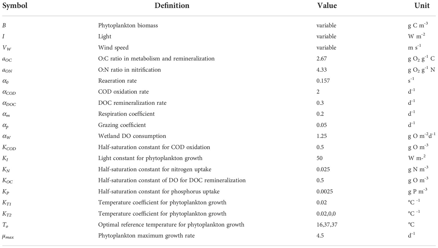
Table 1 Parameter definition, values and units of the water quality model (Cerco and Noel, 2004).

The simulation domain covers the entire Corsica River (Figure 1). Grid resolution is about 100 m at the river mouth to 20 m near the coastline, with 5614 cells, 3159 nodes, and 5 vertical sigma layers. The simulation time step was set at 120 seconds. The model was run for a full year using the 2006 forcing files.

2.2 Data

Solar radiation and long-wave radiation data were downloaded from the Reanalysis V5 (ERA5) of the European Centre for Medium-Range Weather Forecasts (https://www.ecmwf.int/en/forecasts/dataset/ecmwf-reanalysis-v5). Wind, precipitation, air temperature, pressure, and specific humidity data were obtained from the North American Regional Reanalysis domain (NARR; https://www.ncei.noaa.gov/products/weather-climate-models/north-american-regional). ERA5 provides hourly data and NARR provides data for every three hours. Linear interpolation in time was performed on the NARR data to align with the ERA5 data set.

Watershed runoff and associated nutrient loads were generated by using the US EPA Chesapeake Bay Program regulatory watershed model, the Hydrological Simulation Program–FORTRAN (Shenk et al., 2012), calibrated with the USGS River Input Monitoring (RIM) stations on the Chesapeake Bay watershed. There are seven loading points in the Corsica River simulation domain with model forcing on a daily time scale (Figure 1). Open boundary conditions were specified based on the CH3D-ICM (Curvilinear-grid Hydrodynamics 3D Model) simulation in the entire Chesapeake Bay. This modeling system has been used as the Chesapeake Bay regulatory model over the past 30 years and was well calibrated against long-term monitoring data (Cerco and Noel, 2019). The time step in the CH3D-ICM outputs was daily, which was used in specifying the boundary conditions and linear interpolation was performed during the simulation.

The Department of Natural Resource of Maryland (DNR-MD, USA) maintained a monitoring program in the Corsica River and twenty-one discrete sampling events were conducted from April to December 2006. Temperature, salinity and water quality variables including DO and chlorophyll were measured during each sampling event for the three stations used here: the upper estuary station (XHH3851), the mid-estuary station (XHH4931) and lower estuary station (XHH4916) (Figure 1). In addition to the discrete sampling data, high-frequency sensors measuring temperature, salinity (as conductivity), DO and chlorophyll were deployed at the three observation stations for continuous data collection (CONMON). The CONMON sensors record every 15 minutes (https://eyesonthebay.dnr.maryland.gov), but there were numerous interruptions due to sensor malfunctions and extreme weather events. The upper estuary station (XHH3851) has CONMON data for the entire year 2006 (with interruptions), but only from July through December in the mid and lower estuary stations. Furthermore, DNR conducted a sensor-based synoptic survey on July 20, 2006 using DATAFLOW. The sensors recorded every four seconds and the survey lasted about three hours from 8:30 am to 11:30 am with 2886 records in total.

The National Ocean and Atmospheric Administration, USA, maintained surveys on tidal wetlands in Chesapeake Bay (https://coast.noaa.gov). In the Corsica domain, dense tidal wetlands were distributed at the waterhead of all the sub-tributaries, with the largest wetland area located at the upper estuary (Figure 2). We also validated rate processes in the model using direct measurements of sediment oxygen demand (SOD) and sediment-water ammonium fluxes made at three stations in 2006 using in-situ chamber measurements (Boynton et al., 1981; Burdige, 1991; Boynton et al., 2009; Boynton et al., 2018).

FIGURE 2

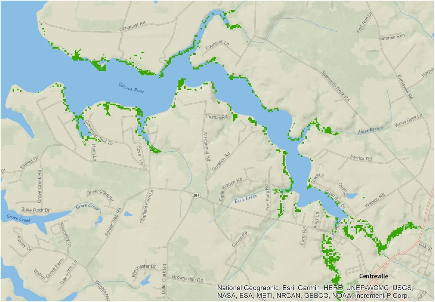
Figure 2 Map of the location of tidal wetlands (green) in the Corsica estuary, which are mostly distributed in the upper estuary and headwaters.

2.3 Data analysis

Data signal analyses were performed on the simulated DO time series to interpret the simulated high frequency variability. The CONMON data had numerous interruptions and signal analyses on the observed time series was not possible. We used Empirical Mode Decomposition (EMD) and spectral analysis using the R programs EMD and Spectrum (Dhiman et al., 2020; Seilmeyer, 2021). EMD, also known as the Hilbert-Huang Transform, is a nonparametric, nonstationary analysis, in which a time series is decomposed into a finite number of intrinsic oscillatory modes using the local maxima and minima envelope (Huang and Wu, 2008; Ezer and Corlett, 2012; Huang et al., 2020). It employs an iterative approach: Once an intrinsic oscillatory mode is determined, it is removed from the initial data set, followed by the second mode computation until all the oscillatory modes are determined. Spectral analysis, on the other hand, is a parametric approach for signal analysis in which the Fourier transformation decomposes a time series into underlying sine and cosine functions of different frequencies (Olson, 1986; Sanford et al., 1990; Fleming et al., 2012). The periodogram quantifies the contributions of the individual frequencies to the time series and the spectrum power density, defined as the amplitude power of the signal, reflects the variance of each signal.

We also applied a Classification and Regression Trees (CART) approach, which is a common type of machine learning algorithm for predictive modeling, to explain how the DO time-series data were related to potential controlling variables in the model. Due to the interruption in the CONMON data and the lack of paired predictor variables, CART was applied to the simulated time series. CART output is a decision tree where each fork is a split in a predictor variable and each end node contains a prediction for the dependent variable (Zhang et al., 2021). CART can statistically demonstrate which factors are particularly important in terms of explanatory power (Morgan, 2014). The R package rpart was used for this analysis (Therneau et al., 2022).

CART can identify and rank key controls on DO, but it remains a binary prediction at each node and does not provide a full time-series prediction. Generalized Additive Model (GAM), on the other hand, can capture nonlinear relationships and provide time-series prediction of the response variable (Hastie and Tibshirani, 1986; Murphy et al., 2022). GAM from the “mgcv” package with cubic regression splines was used (Wood, 2004; Wood, 2006; Harding et al., 2016).

Lastly, DO budgets representing key physical and biological terms were computed with the simulated results at the three stations. The key physical and biogeochemical factors that were analyzed were advective transport (Q), photosynthetic production (P), respiration (R), aeration (A) and sediment oxygen demand (SOD). Aeration affects DO through the sea surface and SOD at the bottom so that integration over the water column is more appropriate for the DO budget computation:

$\begin{array}{ll}\frac{\Delta DO}{\Delta t}=Q+P+R+A+SOD& \text{.(4)}\end{array}$

where ΔDO is the DO change over time span Δt, and Q, P and R are integrated over the water column (no integration is needed for A and SOD). The respiration term includes all processes consuming DO such as phytoplanton resipiration, remineralization of organic material, chemical orxygen demand and nitrification. All these terms were computed and recorded in the output files except the physical transport. Following Du et al. (2018) , physical transport was computed as the difference between ΔDO and other recorded terms. As the model strictly maintains mass balance, the calculation of physical transport is robust. We computed DO budgets at hourly, daily, and annual time scales.

3 Results

3.1 Physical conditions during simulation year

We performed our simulations using realistic forcing for the year 2006. There was a flushing event in the summer of 2006 when freshwater discharge reached to 27 m³ s^-1 and DIN loading up to 4,200 kg N day^-1 (Figure 3A). As shown later, this high loading event had significant impacts on water quality in the Corsica River. Runoff and nutrient loads were elevated earlier in the year and in the fall, but there were two dry periods before and after the summer flushing event (day 60 to 170 and 210 to 240) where river flow was below 2 m³ s^-1. Air temperature showed a typical seasonal cycle: high temperatures up to 36°C in summer and as low as 0°C in winter (Figure 3B). On top of the seasonal cycle, there were higher frequency variations on the order of weeks to a month. Wind was also characterized by high frequency variability, with frequencies in order of hours to days (Figure 3B). Wind speed was higher in winter and fall than in summer. Photosyntheticallyactive radiation (PAR) had both seasonal and diurnal cycles (Figure 3C). Note that PAR remained at an elevated level of about 200 W m^-2 during the day in winter and up to 450 W m^-2 in summer. In addition to the seasonal and diurnal cycles, cloud coverage interrupted the continuous regular variation, causing low radiation from time to time regardless of the season.

FIGURE 3

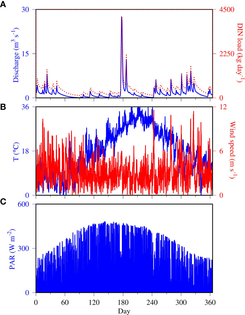
Figure 3 Model forcing data for the calendar year 2006, including (A) Total freshwater discharge (blue line) and dissolved inorganic nitrogen (DIN) load (red dashed line), (B) Air temperature (blue line) and wind speed (red line), and (C) Photosynthetically active radiation (PAR).

3.2 Comparison between simulation and observation

The model successfully reproduced temporal patterns in water temperature at the three observation stations, including both the continuous monitoring data and the cruise sampling data on a bi-weekly and monthly basis (Figures 4A–C). The CONMON data showed high-frequency variability approximately on a weekly time scale, at the upper estuary station (XHH3851) in particular, and the model was able to reproduce these variations in most instances. The maximum water temperature reached up to 35°C in summer and as low as 2°C in winter at the upper estuary station and about 5°C at the mid and lower estuary stations.

FIGURE 4

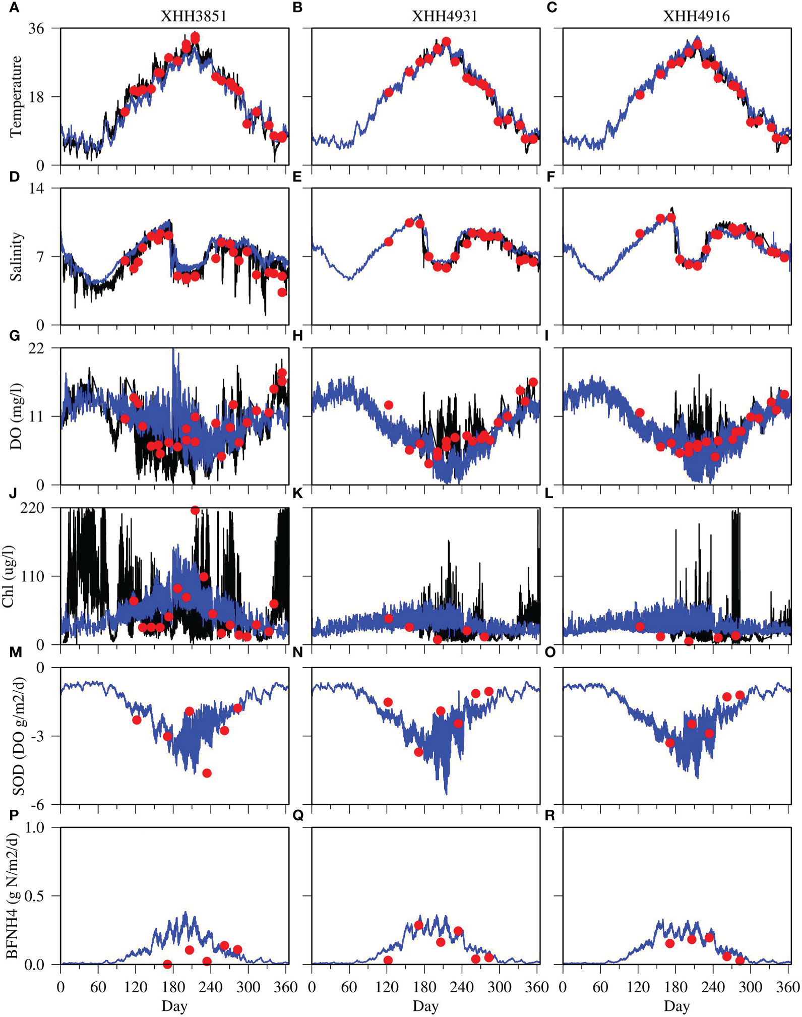
Figure 4 Comparison between model simulations (blue lines) with sensor-based continuous monitoring data (black lines) and cruise-based, discrete samples (red dots) at three observation stations. Each column displays an observation station with XHH3851 on the left, XHH4931 in the middle and XHH4916 on the right. Each row displays a variable with temperature on the top (A–C), followed by salinity (D–F), DO (G–I), chlorophyll (Chl; J–L), sediment oxygen demand (SOD; M-O) and sediment ammonium flux (BFNH4; P–R).

The salinity simulation matched with observations well (Figures 4D–F). Salinity was relatively low in late winter and early spring due to high freshwater discharge, and tended to increase from spring to summer. However, there was a large precipitation event in summer 2006, leading to a significant freshening at all three stations that lasted from July to August. The model reproduced the timing and magnitude of this freshening event but tended to overestimate salinity during several short freshening events in early winter and fall at the upper estuary station (Figure 4D).

The model largely reproduced the observed seasonal and high-frequency variability of DO in summer (Figures 4G–I). DO was higher in the early and late seasons of the year and lower in summer. However, a high productivity event altered this general seasonal pattern, leading to high DO in summer. High-frequency variabilities were particularly visible at the upper estuary station (Figure 4G). The model reproduced most of the variability in both frequency and magnitude of DO but overestimated DO in May and June at this station as compared with the CONMON data. Most of the discrete sampling data were within the simulated range. On the other hand, the model underestimated DO in summer at the mid and lower estuary stations (Figures 4H, I). The model mostly missed the supersaturated DO events in summer at these two stations.

The CONMON data showed large and high-frequency variations in chlorophyll concentrations as well (Figures 4J–L). High-frequency variations were observed throughout the year at the upper estuary station XHH3851 with magnitudes up to 220 μg l^-1. The model has also predicted high-frequency variations in chlorophyll concentration, up to 160 μg l^-1 at the upper estuary station XHH3851 in summer (Figure 4J), but relatively lower variations in other seasons as compared to the CONMON data. The predicted magnitudes of variations in chlorophyll concentration at the mid and lower estuary stations were also lower than that in the CONMON data. The model predicted magnitudes of variations were mostly within 70 μg l^-1 and the magnitudes in the CONMON occasionally reached to 150 μg l^-1 at the mid estuary station (Figure 4K) and up to 200 μg l^-1 at the lower estuary station (Figure 4L).

The model also reproduced the magnitude and seasonal variability of SOD (Figures 4M–O) and sediment-water fluxes of ammonium (Figures 4P–R). The measured average SOD fluxes in summer were 2.23, 1.96, and 2.23 g DO m^-2 d^-1 at the upper, mid, and lower estuary stations, respectively, and the simulated fluxes were 2.36, 2.54 and 2.81 g DO m^-2 d^-1. The model overestimated ammonium fluxes at the upper estuary stations in summer (Figure 4P), but matched the observations at the mid and lower estuary stations. The measured average ammonium fluxes in summer were 0.11, 0.18, and 0.15 g N m^-2 d^-1 at the upper, mid and lower estuary stations, respectively, and the simulated fluxes were 0.17, 0.20 and 0.18 g N m^-2 d^-1. As the diagenesis processes are sensitive to temperature, the sediment fluxes were higher during the summer months than the rest of the year. Similar to the DO simulation, the model predicted high frequency variation in SOD and nutrient sediment fluxes, particularly in summer under low DO conditions.

Patchiness and heterogeneity were common features in both the simulated and observed distribution of DO and chlorophyll (Figure 5). Both DO and chlorophyll were higher in the upper estuary than in the lower estuary. In most cases, the simulation matched well with spatial distributions of the observations but tended to underestimate DO in the mid estuary.

FIGURE 5

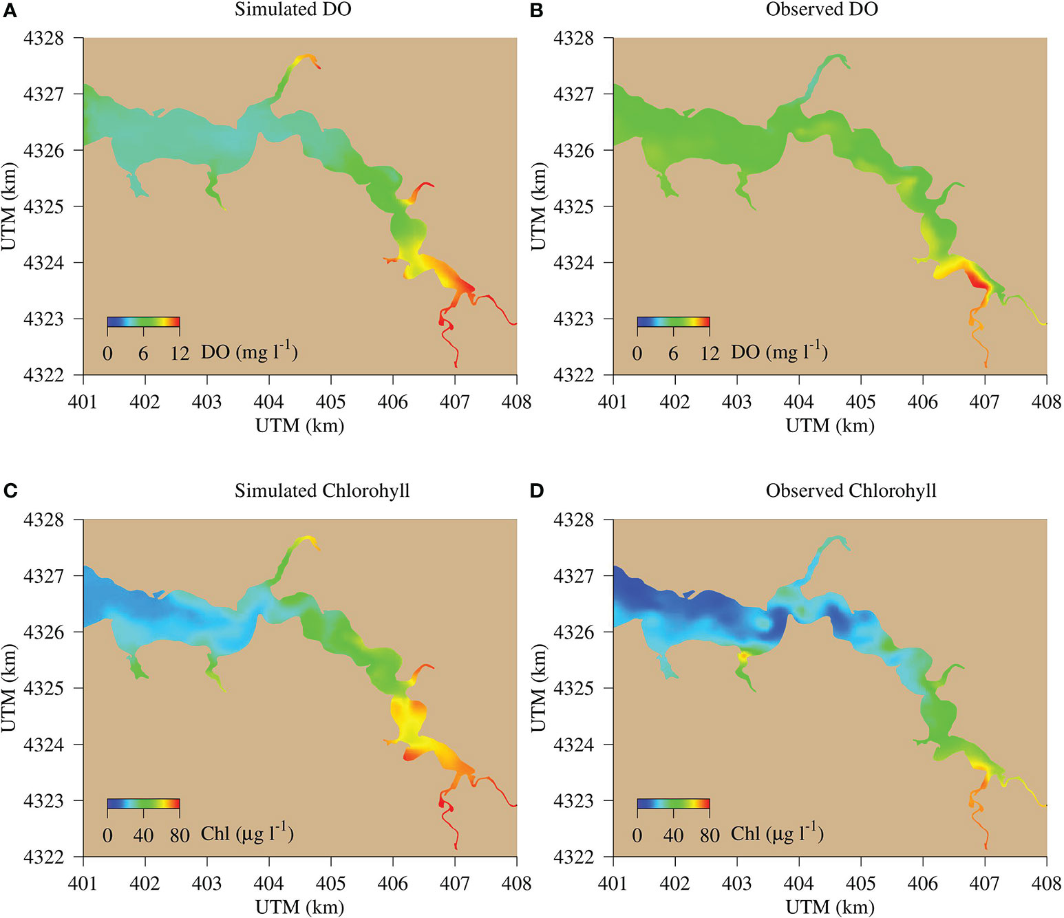
Figure 5 Comparison between model simulations (left panels) with sensor-based synoptic survey data (right panels) for DO (A, B) and chlorophyll (C, D) on July 20, 2006. The survey data were provided by the Department of Natural Resources (DNR) of Maryland and available at https://eyesonthebay.dnr.maryland.gov.

3.3 Signal analysis of the simulated DO time-series

We first explored the magnitude and frequency of modeled DO simulations to identify the timescales at which DO varies most. We concentrate here on the upper estuary station, XHH3851, where high-frequency variations persisted over the entire year. Empirical Model Decomposition (EMD) generated seven modes with different frequencies and periods which all passed the white noise test (Figure 6). The first signal has a period of 12.4 hours, which is the semi-diurnal M2 tidal frequency, while the second signal has a daily period related to diurnal variations. The amplitudes of the diurnal signal were much greater than the semi-diurnal signal. Mode seven has a major period of 121 days, which is coherent with the seasonal cycle, but modified by the summer productive (i.e., high chlorophyll) event resulting from to the large precipitation event. There are four other signals from Mode 3 through Mode 6 with different frequencies and periods, ranging from days to months, but all of them have low amplitudes as compared to the tidal and diurnal variations and thus have lower weights in the composition of the DO time series. Therefore, we focus on mechanisms associated with the frequencies with large contributions.

FIGURE 6

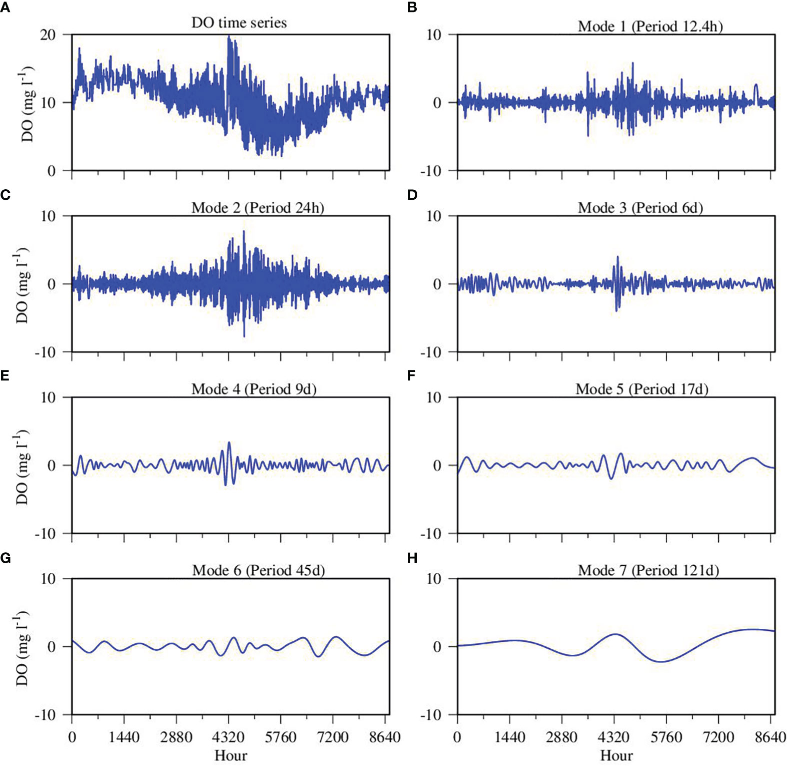
Figure 6 Empirical Mode Decomposition (EMD) of simulated DO time series data at the upper estuary station XHH3851. (A) original time series data; (B) mode 1; (C) mode 2; (D) mode 3; (E) mode 4; (F) mode 5; (G) mode 6; (H) mode 7. The main period of each mode is given in the panel title.

Spectral analysis revealed a similar result as the EMD, where three prominent signals were resolved by the spectral analysis. These signals include: (1) the annual cycle with seasonal variations, (2) the tidal signal with a period of 12.4 hours, and (3) diurnal variation with period of 24 hours (Figure 7). The seasonal variations had the highest spectral power density, but in terms of high-frequency variations, the spectral power density of the diurnal cycle was much higher than the tidal semi-diurnal variations. There were also some poorly resolved low-frequency signals which corresponded to Mode 3 to Mode 6 in the EMD analysis. The results of the two signal analyses were in high degree of coherence, strengthening our interpretation of the DO time-series.

FIGURE 7

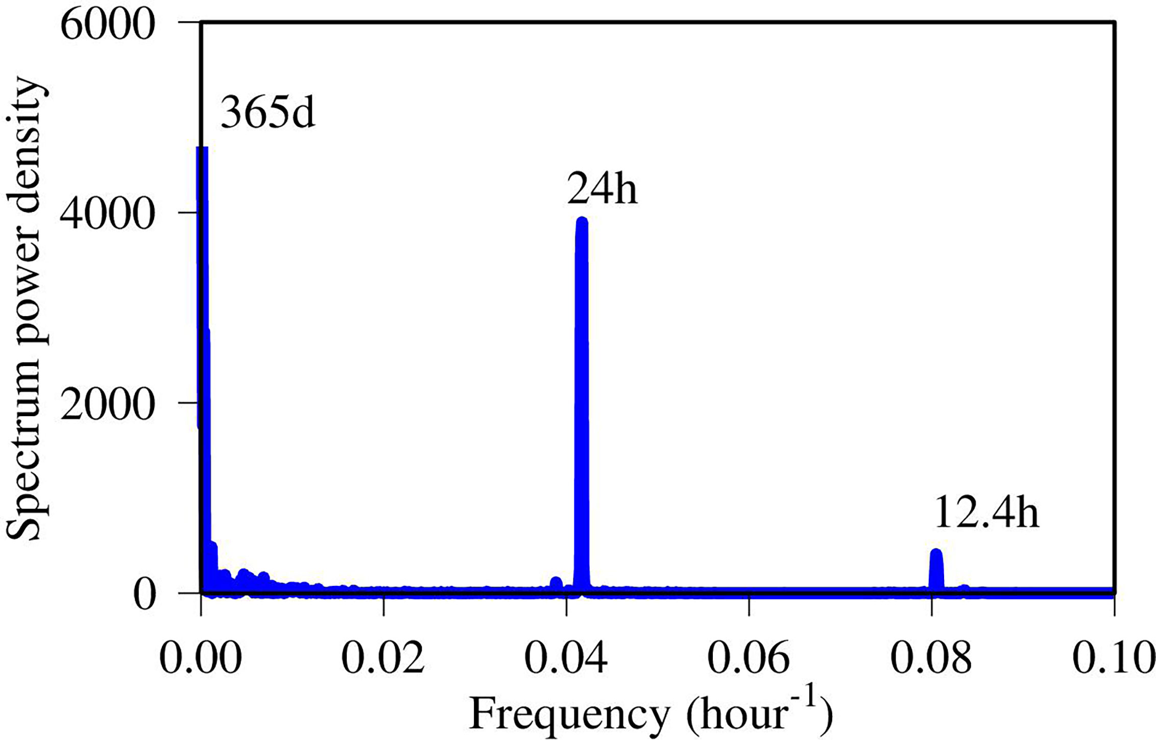
Figure 7 Spectral analysis of the simulated DO time-series data at the upper estuary station XHH3851 (time unit in hours). Notation numbers are the periods.

3.4 Predictability of DO high-frequency variability

CART analysis revealed that water temperature, solar radiation, and chlorophyll were the dominant predictors for DO concentrations (Figure 8). The first node split was defined by water temperature where the average DO concentration was 9.2 mg l^-1 when the temperature was higher than 13°C (58% of the data) and the average DO concentration was 12 mg l^-1 when the water temperature was lower than 13°C (42% of the data). The second node split was defined by solar radiation where the average DO concentration was 8 mg l^-1 when the solar radiation was lower than 234 W m^-2 and 11 mg l^-1 when the solar radiation was above 234 W m^-2. On the right-hand side of the tree, the second category was also split further by temperature. On the third category, three of the four nodes were split by chlorophyll with 66% of the total data population. Sea surface elevation (tide) played a role in the fourth node splitting. There were fourteen node splits in total, of which six were associated with temperature and five with chlorophyll.

FIGURE 8

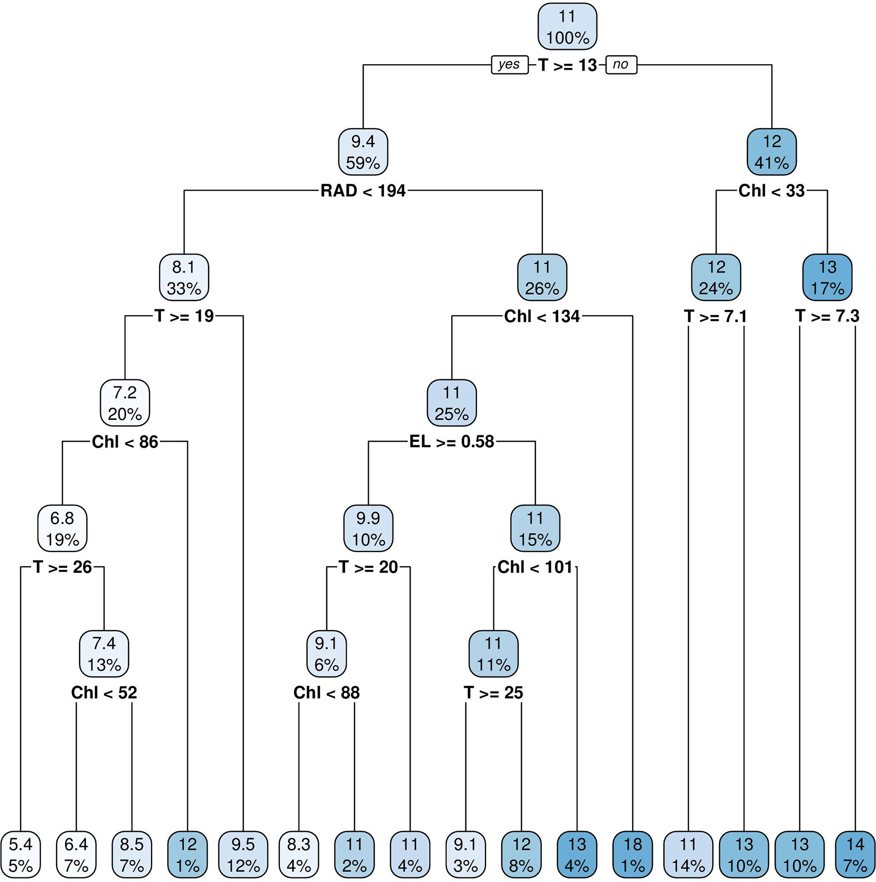
Figure 8 Classification And Regression Tree (CART) analysis of DO simulation time-series data at the upper estuary station XHH3851. Independent variables are water temperature (T), chlorophyll concentration (Chl), sea surface elevation (EL) and solar radiation (RAD).

The GAM predicted 93% of the variance of the DO time series data using the same predictors as in the CART analysis (Figure 9). The power of GAM resides in its ability to capture nonlinear relationships between the dependent variable and the predictors (Figure 10). Overall, temperature had a negative relationship with DO (Figure 10A) and chlorophyll had a positive relationship with DO (Figure 10B). But between chlorophyll concentrations of 40 and 60 μg l^-1, DO declined with increasing chlorophyll, which was a notable departure from the general positive relationship. Both tidal elevation and nutrient load had generally a negative relationship with DO (Figures 10C, D). DO was relatively insensitive to tides at high tidal levels, and insensitive to loads at the low end of nutrient load. Solar radiation had a general positive relationship with DO (Figure 10E). Hour of the day (HOD) was designed to capture the diurnal variations and the fitted GAM spline function was basically as expected (Figure 10F), where DO concentrations were higher during the day and lower in the night. As a common feature, all the relationships are nonlinear.

FIGURE 9

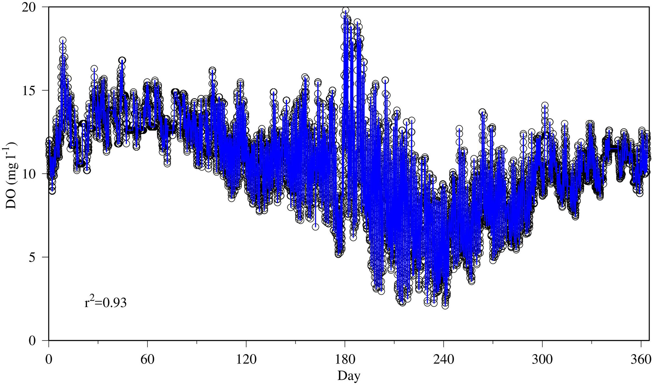
Figure 9 Generalized Additive Model (GAM) prediction (blue line) of DO simulation time-series data (black circles) at the upper estuary station XHH3851 using the same prediction variables used in the CART analysis (Figure 8).

FIGURE 10

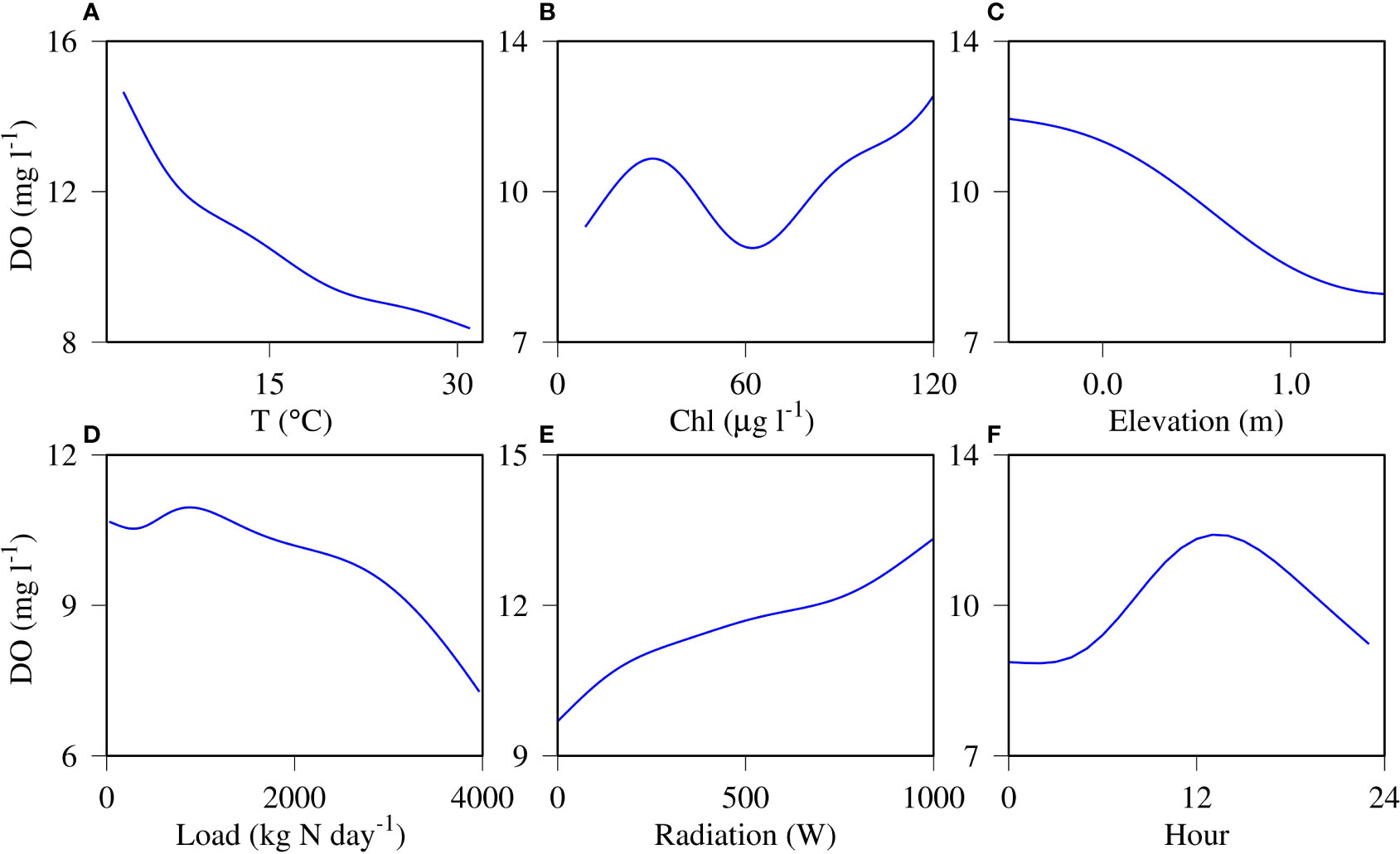
Figure 10 Generalized Additive Model (GAM) fitted function of each predictor (x axis) in predicting DO concentration (y axis) for water temperature (A), chlorophyll-a (B), sea surface elevation (C), nitrogen loading (D), solar radiation (E) and hour of the day (F).

3.5 DO budget over temporal and spatial scales

Budget analysis of hourly model output suggested that physics (including both advection and eddy diffusion) accounted for 43% of DO variation at the upper estuary station XH3851 (Table 2), followed by respiration (22%), photosynthesis (19%), aeration (12%) and SOD (5%). Moreover, the physical contribution increased to 59% at the lower estuary station (XHH4916) where the physical impact was larger than the total of other processes. However, the physical contribution decreased with time scales. The physics contribution decreased from 43% at the hourly scale to 16% on the daily scale, and only 7% on the annual scale at the upper estuary station XHH3851. On daily and annual scales, both photosynthetic production and respiration were higher than the physical contribution at the upper and mid estuary stations, but physics remained higher than photosynthetic production at the lower estuary station.

TABLE 2

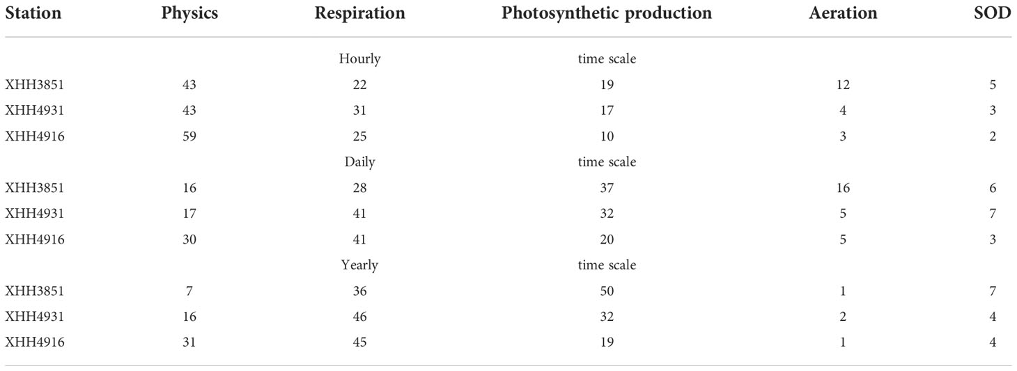
Table 2 Percent contribution (%) to DO budget across different time scales and stations (SOD: Sediment Oxygen Demand).

4 Discussion

4.1 Physical impacts on DO variability

Our model simulation and associated signal analyses revealed that physical transport is a primary driver of DO variability on hourly timescales in the shallow Corsica River system. These tidal-scale impacts on DO variability reflect that mixing and advection of DO across space is an important feature of hourly-scale DO variability (e.g., Duvall et al., 2022). The transfer of DO signals across space depends on the heterogeneity in DO distribution, and both our simulation and the synoptic surveys showed that heterogeneity is a strong characteristic in DO distribution (Figure 5). These heterogeneous conditions emerge from strong spatial patterns of phytoplankton biomass, as well as interactions between the coastline and current that drive changes in current velocity and direction. For example, Tian (2019) and Tian (2020) found that interactions between physics and coastline meanders can generate complex advection features that fundamentally alter biogeochemical processes and water quality properties in the Chester River. Helical advection resulting from interactions between currents and the coastline can interrupt saltwater intrusion, vertical diffusivity, phytoplankton development and DO distribution. The Corsica River has geometry even more complex and shallower than the connected Chester River estuary, and simulated surface currents on July 20, 2006 reveal eddies, meanders, and filaments with spatial scales in the order of kilometers to tens of kilometers (Figure 11). The complex flow field generates patchy distributions in DO and chlorophyll. Thus, the bidirectional tidal current flowing back and forth will lead to high tidal-scale variations in DO and chlorophyll concentrations at a fixed station, which explains the tidal-frequency variability shown in both EMD and spectral analyses.

FIGURE 11

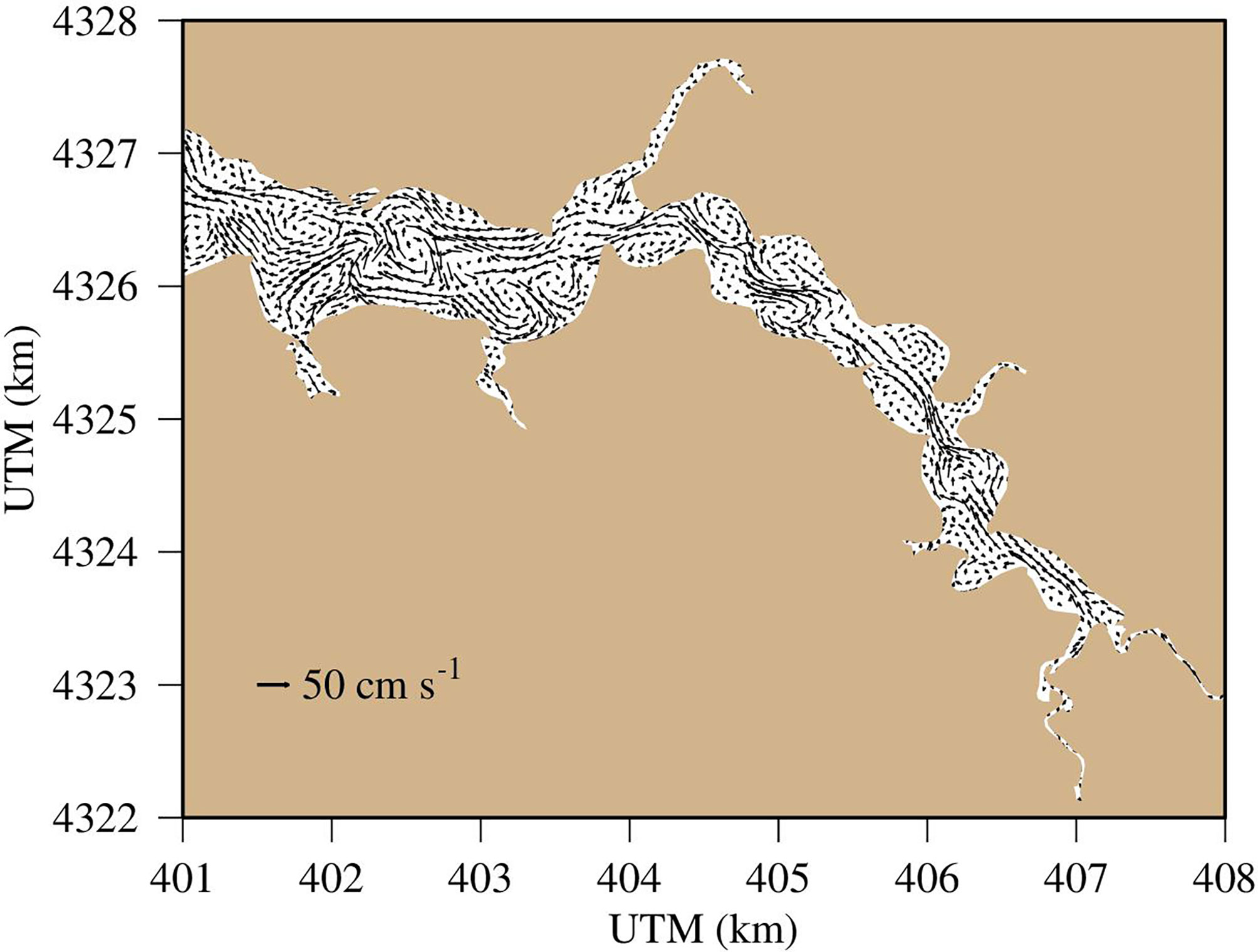
Figure 11 Simulated surface current on July 20, 2006.

Tidal advection can be cyclic, the effect of which can be balanced out between the opposite tidal phases (flooding and ebb tide). As an example, the tidal effect is illustrated for 10 days (July 1-10) together with other processes affecting DO concentration (Figure 12). Tidal fluxes of DO are cyclic between positive and negative within a tidal cycle. When computed on a daily basis, the tidal effect on DO is largely balanced out between the two tidal phases, which explains the smaller contribution of physics to DO variability on a daily basis than on hourly time scales. Two additional factors can affect the DO budget with a tidal cycle: Residual current and stability of the spatial gradient. If a residual current exists, water mass advection may not be balanced between the two phases of the tide. If the gradient is not stable, the advected quantity of DO will differ as well. The two factors can act in the same direction (strengthen each other) or the opposite (reducing their effect). As a result, the physical effect is not the simple linear equation that can be easily predicted in a real shallow water system. The spatial variation in physics contribution to DO variability (Table 2) can be explained by the difference in residual current and gradient stability.

FIGURE 12

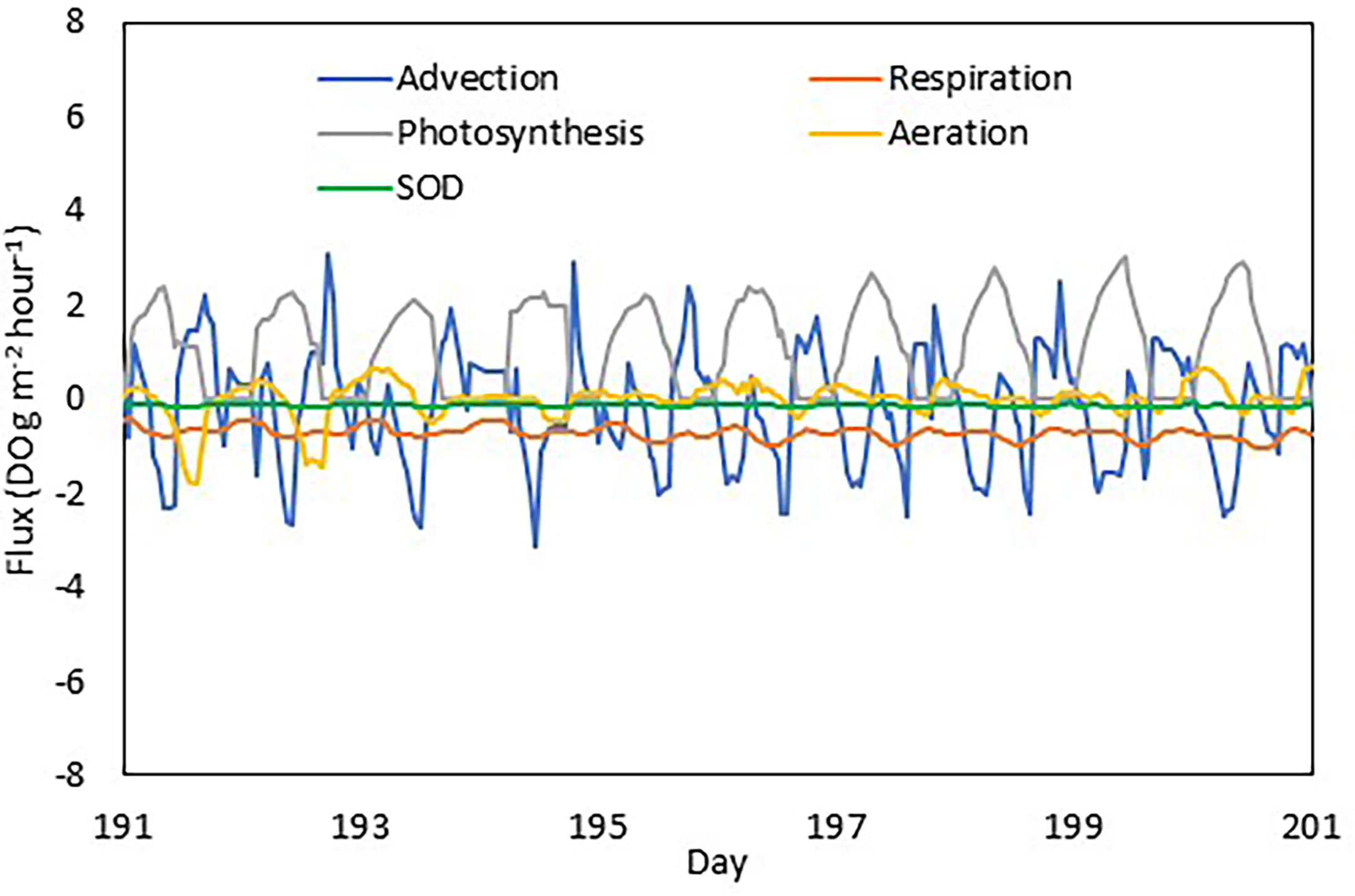
Figure 12 DO fluxes from different processes at the upper estuary station XHH3851. Advection, photosynthesis and respiration are integrated in the water column, aeration is at the sea surface and sediment oxygen demand at the bottom.

4.2 Biogeochemical impact on high frequency variability

Even though tide is a primary driver of variability at sub-diurnal frequencies, biogeochemical processes are the dominant drivers for diurnal variations. This can be ascribed to the net primary production during the day, respiration during the night, and aeration that responds to under- and super-saturation associated with metabolism. Primary production is the dominating factor that generates DO, and it also stimulates high respiration during the day as well as during the night (Figure 12), forming a diurnal cycle of net DO production during the day and consumption during the night. Unlike the tidal effects that are cyclic during a day, DO production through photosynthesis is accumulative over time, explaining its increasing weight in the DO budget on longer time scales. Moreover, biogeochemical processes significantly contribute to the spatial variability as well. On top of the patches in distribution caused by eddies, both DO and chlorophyll have relatively elevated concentrations in the upper estuary (Figure 5). Turbidity limits phytoplankton growth in the water head and nutrients become limiting in the lower estuary so that phytoplankton growth peaks in the upper estuary, leading to both high chlorophyll and DO concentration (Tian et al., 1993). Even though SOD has a fairly regular seasonal cycle, there are high-frequency variations in SOD (daily-weekly scale) associated with variations in temperature, organic matter variability, algal growth and DO concentration in the overlying water.

4.3 Relationship between DO and environmental factors

Temperature is a major predictor of DO in the shallow Corsica River system. Temperature influence on DO solubility is a major mechanism in determining their relationship (Najjar et al., 2010; Li et al., 2015; Irby et al., 2018). Temperature not only influences DO solubility, but also respiration and biogeochemical processes. Tian et al. (2021) reported that under future climate warming conditions, decreasing solubility under higher temperatures contributes 55% of the total DO decrease in the Chesapeake Bay, whereas biological processes contribute 33% and change in stratification 9%. Stratification is absent in the shallow systems so that solubility and biological processes primarily determine the relationship between DO and temperature.

The positive chlorophyll-DO relationship (Figure 10B) indicates that photosynthetic production of DO is crucial to determine DO dynamics in shallow systems. Du et al. (2018) also reported that chlorophyll is a good predictor of DO. The decreasing trend of DO around 60 μg l^-1 chlorophyll concentration represents a departure from this general relationship under specific environmental conditions. During some periods of the summer, mineralization of organic matter or other environmental factors decrease DO regardless of DO production through photosynthesis. In fact, high chlorophyll concentration occurred during the summer due to increased nutrient loading and nutrient fluxes from the sediment (Figures 2 and 4P–R). During this period, water temperature was around 30 °C. Such high temperatures can accelerate the remineralization of organic substances and subsequently increase DO consumption, overwhelming DO production through photosynthesis. This phenomenon shows the degree of complexity and interactions between different processes in determining water quality in the coastal shallow water systems. Generally, high chlorophyll in these systems can buoy DO, however, high chlorophyll is also an indicator of respiration potential and temperature helps mediate whether high chlorophyll is a net negative or positive in the DO balance.

The negative relationship between tide and DO at the upper estuary station depends on the location of the station within the estuarine system. DO was relatively lower in the mid estuary than in the upper estuary (Figure 5). High tide brought water from the mid estuary to this station and low tide brought in water from the upper estuary, forming the negative relationship between DO and tide. The negative relationship between nutrient loading and DO is as expected, given that nutrient loading fuels eutrophication and hypoxia in coastal and estuarine systems. Solar radiation is a primary diver in determining DO in the Corsica River, revealed by the CART analysis. The continuous positive relationship between DO and solar radiation indicates that light is a limiting factor and did not reach to a saturation level. Similar relationships between DO variability and daily variability in PAR have been found in the Delaware Inland Bays (Tyler et al., 2009), where multiple cloudy days under warm temperatures lead to hypoxia.

GAM output allowed us to quantify the relative role of multiple, sometimes competing processes in impacting DO variability. GAM minimizes the generalized cross validation score (GCV) for parameter selection and prediction, and GCV can be used as a measure of prediction power for individual variables, where the estimation errors with lower values indicate higher prediction power. Based on the GCV values, water temperature has the highest prediction power, followed by tide, chlorophyll, solar radiation, wind speed and nutrient loads. The highly ranked tide effect in the Corsica River is similar to results found for the Caloosahatchee River (Florida, USA) and Perdido Bay (Alabama, USA), where tide was found to be a major factor in determining DO concentration (Xia et al., 2010; Xia et al., 2011; Xia and Jiang, 2015). However, the lower ranked wind forcing in the Corsica River differs from the two latter shallow water systems where both wind speed and direction have significant effect of DO variation. Because the Corsica River is a small system (6 km long) compared to the Caloosahatchee River (45 km) and Perdido Bay (30 km), wind fetch is always limited is the Corsica River. The low rank of nutrient loading may be surprising, but it only reflects the impact of loads on DO within a given year, which contrasts with other studies that relate inter-annual changes in nutrient loading to DO depletion.

4.4 Model limitation and future development

The model was able to simulate high frequency variability in both DO and chlorophyll similar to that observed in the CONMON data. However, the variability and magnitude of modeled chlorophyll was lower than the CONMON data, particularly in the simulation at the upper estuary stations. The discrete chlorophyll measurements did compare well with model estimates in this region (Figure 4J), so there remains an open question about the mismatch between modeled chlorophyll and the sensor-based measures. The chlorophyll content of phytoplankton is complex, with the carbon to chlorophyll (C:Chl) ratio changing with growth phase, photoacclimation, diurnal changes in photosynthesis, and dominant algal species (Carberry et al., 2019; Masuda et al., 2021). However, a constant ratio was used in the simulation (C:Chl=25), suggesting that a dynamic C:Chl may help improve future simulations. Also, chlorophyll sensors are based on fluorescence and the fluorescence of chlorophyll can change up to an order of magnitude due to quenching effect and across difference species for which the model does not have corresponding parameterization (Falkowski and Kolber, 1995; Sackmann et al., 2008; Carberry et al., 2019). Other autotrophs are present in shallow coastal systems in addition to phytoplankton. For example, vertically migrating phytoplankton are common in this region, and the passing of a thin layer of cells by the sensor could cause a rapid increase in fluorescence that would not be captured in our model. Benthic microalgae and their resuspension have the potential to alter observed autotrophic biomass and chlorophyll concentration. Kemp et al. (2005) estimated that benthic microalgae production accounted for 10-30% of phytoplankton production in the upper Chesapeake Bay, which can significantly alter sediment fluxes of nutrients and organic matter (Cerco and Seitzinger, 1997; Tyler et al., 2003). Submerged aquatic vegetation (SAV) can complicate biogeochemical cycles and the function of shallow systems. A recent study using the CH3D-ICM modeling system revealed that SAV can take up nutrients from sediment and release organic and inorganic materials to the water column (Carl Cerco, personal communication, April 6, 2022). Tidal wetlands can have similar effects. All benthic autotrophs have diurnal cycles leading to high frequency variations in the water column. The model also underestimated DO supersaturation during summer daytime periods. While high DO is not as crucial to simulate as low DO, which can be fatal to marine life, missing high daily DO may indicate conventional models need structural change to capture diel-cycling hypoxia. Specifically, reaeration schemes that are spatially variable may be necessary to account for differences in fetch within small systems and more refined information on the respiration of the organic matter pool in shallow waters with large allochthonous inputs compared to open mainstream bay stations may be necessary.

5 Conclusion

Our model simulation reproduced high-frequency variability in DO and chlorophyll that matched that observed in sensor-based continuous monitoring data. Signal analysis showed that there are two major modes in the high-frequency variation of DO: semi-diurnal M2 tidal frequency and diurnal frequency. The diurnal spectral power density is much higher than the semi-diurnal tidal signal, implying that biogeochemical processes dominate over physical transport in determining high-frequency variability, particularly by the net photosynthesis production during the day and respiration in the night. However, physical transport contributes to DO variability on an hourly time scale and the tidal signal is significant. The simulated flow field is dominated by eddies and meanders, which lead to patchiness and heterogeneity in the distribution of water quality properties. Biogeochemical processes also generate heterogeneous distribution with higher DO and chlorophyll in the upper estuary and lower in the mid estuary. Temperature, chlorophyll, and solar radiation are the major predictors of DO in the Corsica River, with temperature having larger impacts on low DO in summer whereas chlorophyll accounts for DO supersaturation conditions during phytoplankton blooms. Changes in DO solubility and biological rate are the major mechanisms in determining the DO-temperature relationship. Chlorophyll has a positive relationship with DO, indicating that photosynthetic production dominates their relationship. The continuous increase in DO with solar radiation indicate that light is a limiting factor in photosynthetic production in the Corsica River. Our study shows that a high-resolution, unstructured grid model has the potential to resolve complex physical and biological dynamics governing water quality in shallow water systems. We also demonstrated how machine learning approaches can be helpful in analyzing complex numerical model output to decipher the complex interactions among numerous forcing factors in shallow water systems.

Data availability statement

The raw data supporting the conclusions of this article will be made available by the authors, without undue reservation.

Author contributions

RT, XC, JT, DB, CC, and LL contributed to conception and design of the study. RT and JT organized the database. RT performed the model operation and statistical analysis. RT wrote the first draft of the manuscript. JT, CC, DB, CC, and LL wrote sections of the manuscript. All authors contributed to the article and approved the submitted version.

Acknowledgments

The authors thank the Chesapeake Bay Program and UMCES IAN for providing funding (CB-75230480), the Chesapeake Research Consortium for providing funding (CB96343601) and the Maryland Department of Natural Resource for providing the Continuous Monitoring data. This project was also supported in part by an appointment to the Research Participation Program at the Chesapeake Bay Program Office, U.S. Environmental Protection Agency, Region 3 administered by the Oak Ridge Institute for Science and Education through an interagency agreement between the U.S. Department of Energy and U.S. Environmental Protection Agency. Special thanks go to the Chesapeake Bay Program Modeling Team for their enthusiastic helps, particularly Gary Shenk, Gopal Bhatt, Bill Dennison and Dave Nemazie, and two reviewers for their constructive comments. This is UMCES Contribution No. 6234 and Ref. No. [CBL] 2023-029.

Conflict of interest

The authors declare that the research was conducted in the absence of any commercial or financial relationships that could be construed as a potential conflict of interest.

Publisher’s note

All claims expressed in this article are solely those of the authors and do not necessarily represent those of their affiliated organizations, or those of the publisher, the editors and the reviewers. Any product that may be evaluated in this article, or claim that may be made by its manufacturer, is not guaranteed or endorsed by the publisher.

References

Boynton W. R. (1997). “Chesapeake Bay eutrophication current status, historical trends, nutrient limitation and management actions,” in Proceedings of the coastal nutrients workshop (Artamon, Australia: Australian Water &Wastewater Association Incorporated), 6–13.

Google Scholar

Boynton W. R., Ceballos M. A. C., Bailey E. M., Hodgkins C. L. S., Humphrey J. L., Testa J. M. (2018). Oxygen and nutrient exchanges at the sediment-water interface: A global synthesis and critique of estuarine and coastal data. Estuar. Coasts 41, 301–333. doi: 10.1007/s12237-017-0275-5

CrossRef Full Text | Google Scholar

Boynton W. R., Kamp W. M., Osborne C. G., Kaumeyer K. R., Jenkins C. (1981). Influence of water circulation rate on in situ measurements of benthic community respiration. Mar. Biol. 65, 185–190. doi: 10.1007/BF00397084

CrossRef Full Text | Google Scholar

Boynton W. R., Testa J. M., Kamp W. M. (2009). An ecological assessment of the Corsica river estuary and watershed scientific advice for future water quality management (Annapolis: Maryland Department of Natural Resource, Technical Report Series No. TS-587-09).

Google Scholar

Brady D. C., Targett T. E. (2010). Characterizing the escape response of air-saturation and hypoxia-acclimated juvenile summer flounder (Paralichthys dentatus) to diel-cycling hypoxia. J.Fish Biol. 77, 137–152.

PubMed Abstract | Google Scholar

Brady D. C., Targett T. E. (2013). Movement of juvenile weakfish (Cynoscion regalis) and spot (Leiostomus xanthurus) in relation to diel-cycling hypoxia in an estuarine tributary: Assessment using acoustic telemetry. Mar. Ecol. Prog. Ser. 491, 199–219. doi: 10.3354/meps10466

CrossRef Full Text | Google Scholar

Brady D. C., Testa J. M., Toro D. M. D., Boynton W. R., Kemp W. M. (2013). Sediment flux modeling: calibration and application for coastal systems. Estuar. Coast. Shelf Sci. 117, 107–124. doi: 10.1016/j.ecss.2012.11.003

CrossRef Full Text | Google Scholar

Burdige D. J. (1991). The kinetics of organic matter mineralization in anoxic marine sediments. J. Mar. Res. 49, 727–761. doi: 10.1357/002224091784995710

CrossRef Full Text | Google Scholar

Cai X., Shen J., Zhang Y. J., Qin Q., Wang Z., Wang H. (2021). Impacts of sea-level rise on hypoxia and phytoplankton production in Chesapeake bay: Model prediction and assessment. J. Am. Water Resour. Assoc. 58 doi: 10.1111/1752-1688.12921

CrossRef Full Text | Google Scholar

Cai X., Zhang J. Y., Shen J., Wang H., Wang Z., Qin Q., et al. (2020). A numerical study of hypoxia in Chesapeake bay using an unstructured grid model: Validation and sensitivity to bathymetry representation. J. Am. Water Resour. Assoc. 58 doi: 10.1111/1752-1688.12887

CrossRef Full Text | Google Scholar

Carberry L., Roesler C., Drapeau S. (2019). Correcting in situ chlorophyll fluorescence time-series observations for nonphotochemical quenching and tidal variability reveals nonconservative phytoplankton variability in coastal waters. Limnol. Oceanogr. 17, 462–473. 10.1002/lom3.10325

Google Scholar

Carstensen J., Andersen J. H., Gustafsson B. G., Conley D. J. (2014). Deoxygenation of the Baltic Sea during the last century. Proc. Natl. Acad. Sci. 111, 5628–5633. doi: 10.1073/pnas.1323156111

CrossRef Full Text | Google Scholar

Cerco C. F., Cole T. M. (1994). CE-QUAL-ICM: a three-dimensional eutrophication model, version 1.0. user’s guide. Ed. Vicksburgh M. S. (Annapolis: U.S. Army Corps of Engineers Waterways Experiments Station).

Google Scholar

Cerco C. F., Noel M. R. (2004). The 2002 Chesapeake bay eutrophication model. EPA 903-R-04-004 (Annapolis, Maryland: U.S. Environmental Protection Agency, Chesapeake Bay Program Office).

Google Scholar

Cerco C. F., Noel M. R. (2019). “2017 Chesapeake bay water quality and sediment transport model,” in A report to the US environmental protection agency Chesapeake bay program office December 2019 final report Annapolis, 580.

Google Scholar

Cerco C. E., Seitzinger P. (1997). Measured and modeled effects of benthic algae on eutrophication in Indian river-rehoboth bay, Delaware. Estuaries 20, 231–248. doi: 10.1111/1752-1688.12919

CrossRef Full Text | Google Scholar

Cerco C. F., Tian R. (2021). Impact of wetlands loss and migration, induced by climate change, on Chesapeake bay DO standards. J. Am. Water Resour. Assoc 58. doi: 10.1111/1752-1688.12919

CrossRef Full Text | Google Scholar

Dhiman H. S., Deb D., Balas V. E. (2020). Hybrid machine intelligent wind speed forecasting models (Oxford: Elsevier Inc), 50.

Google Scholar

Diaz R. J., Rosenberg R. (2008). Spreading dead zones and consequences for marine ecosystems. Science 321, 926–929. doi: 10.1126/science.1156401

PubMed Abstract | CrossRef Full Text | Google Scholar

Di Toro D. M. (2001). Sediment flux modeling (Oxford, U.K.: Wiley), 656.

Google Scholar

Du J. B., Shen J., Park K., Wang Y. P., Yu X. (2018). Worsened physical condition due to climate change contributes to the increasing hypoxia in Chesapeake bay. Sci. Total Environ. 630, 707–717. doi: 10.1016/j.scitotenv.2018.02.265

PubMed Abstract | CrossRef Full Text | Google Scholar

Duvall M. S., Jarvis B. M., Hagy J. D. III, Wan Y. S. (2022). Effects of biophysical processes on diel−cycling hypoxia in a subtropical estuary. Estuar. Coasts 45, 1615–1630. doi: 10.1007/s12237-021-01040-y

CrossRef Full Text | Google Scholar

Ezer T., Corlett W. B. (2012). Is sea level rise accelerating in the Chesapeake bay? a demonstration of a novel new approach for analyzing sea level data. Geophys. Res. Lett. 39, L19605. doi: 10.1029/2012GL053435

CrossRef Full Text | Google Scholar

Falkowski P., Kolber Z. (1995). Variations in chlorophyll fluorescence yields in phytoplankton in the world oceans. Funct. Plant Biol. 2, 341–355. doi: 10.1071/PP9950341

CrossRef Full Text | Google Scholar

Fleming S. W., Lavenue A. M., Aly A. H., Adams A. (2012). Practical applications of spectral analysis to hydrologic time series. Hydrol. Process. 16, 565–574. doi: 10.1002/hyp.523

CrossRef Full Text | Google Scholar

Frankel L. T. (2021). “Quantifying the increased resiliency of Chesapeake bay hypoxia to environmental conditions: A benefit of nutrient reductions,” in Dissertations, master theses (Gloucester Point: William & Mary), 1638386508. Available at: https://scholarworks.wm.edu/etd/1638386508.

Google Scholar

Graziano A. P., Jones R. C. (2017). Diel and seasonal patterns in continuously monitored water quality at fixed sites in two adjacent embayments of the tidal freshwater potomac river. Water 9, 624. doi: 10.3390/w9080624

CrossRef Full Text | Google Scholar

Hagy J. D., Boynton W. R., Keefe C. W., Wood K. V. (2004). Hypoxia in Chesapeake Bay 1950-2001: Long-term change in relation to nutrient loading and river flow. Estuaries 27, 634–658. doi: 10.1214/ss/1177013604

CrossRef Full Text | Google Scholar

Hale S. S., Cicchetti G., Deacutis C. F. (2016). Eutrophication and hypoxia diminish ecosystem functions of benthic communities in a new England estuary. Front. Mar. Sci 29. doi: 10.3389/fmars.2016.00249

CrossRef Full Text | Google Scholar

Harding J. L. W., Gallegos C. L., Perry E. S., Mille W. D., Adolf J. E., Mallonee M. E., et al. (2016). Long-term trends of nutrients and phytoplankton in Chesapeake bay. Estuar. Coasts 39, 664–681. doi: 10.1007/s12237-015-0023-7

CrossRef Full Text | Google Scholar

Hastie T., Tibshirani R. J. (1986). Generalized additive models. Stat. Sci. 1, 297–318.

Google Scholar

Howarth R., Chan F., Conley D. J., Garnier J., Doney S. C., Marino R., et al. (2011). Coupled biogeochemical cycles: Eutrophication and hypoxia in temperate estuaries and coastal marine ecosystems. Front. Ecol. Environ. 9 (1), 18–26. doi: 10.1890/100008

CrossRef Full Text | Google Scholar

Huang W. C., Chu T. Y., Jhan. Y. S., Lee J. L. (2020). Data synthesis based on empirical mode decomposition. J. Hydrol. Eng. 25 (7), 04020028. doi: 10.1061/(ASCE)HE.1943-5584.0001935

CrossRef Full Text | Google Scholar

Huang N. E., Wu Z. (2008). A review on Hilbert-Huang transform: Method and its applications to geophysical studies. Rev. Geophys. 46, 1–23. doi: 10.1029/2007RG000228

CrossRef Full Text | Google Scholar

Irby I. D., Friedrichs M. A. M., Fei D., Hinson K. E. (2018). The competing impacts of climate change and nutrient reductions on dissolved oxygen in Chesapeake bay. Biogeosciences 15, 2649–2668. doi: 10.5194/bg-15-2649-2018

CrossRef Full Text | Google Scholar

Jassby A., Platt T. (1976). Mathematical formulation of the relationship between photosynthesis and light for phytoplankton. Limnol Oceanogr 21, 540–547. doi: 10.4319/lo.1976.21.4.0540

CrossRef Full Text | Google Scholar

Kemp W. M., Boyton W. R., Adolf J. E., Boesch D. F., Boicourt W. C. (2005). Eutrophication of Chesapeake bay: Historical trends and ecological interactions. Mar. Ecol. Prog. Ser. 303, 1–29. doi: 10.3354/meps303001

CrossRef Full Text | Google Scholar

Li Y., Li M., Kemp W. M. (2015). A budget analysis of bottom-water dissolved oxygen in Chesapeake bay. Estuar. Coasts 38. doi: 10.1007/s12237-014-9928-9

CrossRef Full Text | Google Scholar

Linker L. C., Batiuk R. A., Shenk G. W., Cerco C. F. (2013). Development of the Chesapeake bay watershed total maximum daily load allocation. J. Am. Water Resour. Assoc. 49, 986–1006. doi: 10.1111/jawr.12105

CrossRef Full Text | Google Scholar

Masuda Y., Yamanaka Y., Smith H. L., Hirata T., Akano H., Oka A., et al. (2021). Photoacclimation by phytoplankton determines the distribution of global subsurface chlorophyll maxima in the ocean. Nature 594. doi: 10.1038/s43247-021-00201-y

CrossRef Full Text | Google Scholar

McGlathery K. J., Reidenbach M. A., D’Odorico P., Fagherazzi S., Pace M. L., Porter J. H. (2013). Nonlinear dynamics and alternative stables states in shallow coastal systems. Oceanography 26, 220–231. doi: 10.1016/j.ecss.2009.09.026

CrossRef Full Text | Google Scholar

Morel F. (1983). Principles of aquatic chemistry (New York, NY, USA: John Wiley and Sons).

Google Scholar

Morgan J. (2014). Classification and regression tree analysis. Boston univ., technical report no. 1 Boston.

Google Scholar

Murphy R. R., Keisman J., Harcum J., Karrh R. R., Lane M., Perry E. S., et al. (2022). Nutrient improvements in Chesapeake bay: Direct effect of load reductions and implications for coastal management. Environ. Sci. Technol. 56, 260–270. doi: 10.1021/acs.est.1c05388

PubMed Abstract | CrossRef Full Text | Google Scholar

Murphy R. R., Kemp W. M., Ball W. P. (2011). Long-term trends in Chesapeake bay seasonal hypoxia, stratification, and nutrient loading. Estuar. Coasts 34, 1293–1309. doi: 10.1007/s12237-011-9413-7

CrossRef Full Text | Google Scholar

Najjar R. G., Pyke C. R., Adams M. B., Breitburg D., Hershner C., Kemp M., et al. (2010). Potential climate change impacts on the Chesapeake bay. Estuar. Coast. Shelf Sci. 86, 1–20. doi: 10.1016/j.ecss.2009.09.026

CrossRef Full Text | Google Scholar

Neubauer S., Anderson I. (2003). Transport of dissolved inorganic carbon from a tidal freshwater marsh to the York river estuary. Limnol. Oceanogr. 48, 299–307. doi: 10.4319/lo.2003.48.1.0299

CrossRef Full Text | Google Scholar

Newcombe C. L., Horne W. A. (1938). Oxygen-poor waters of the Chesapeake bay. Science 88, 80–81. doi: 10.1126/science.88.2273.80

PubMed Abstract | CrossRef Full Text | Google Scholar

Ni W., Li M., Testa J. M. (2020). Discerning effects of warming, sea level rise and nutrient management on long-term hypoxia trends in Chesapeake bay. Sci. Total Environ. 737, 139717. doi: 10.1016/j.scitotenv.2020.139717

PubMed Abstract | CrossRef Full Text | Google Scholar

Olson P. (1986). The spectrum of subtidal variability in Chesapeake bay circulation. Estuar. Coast. Shelf Sci. 3, 527–550. doi: 10.1016/0272-7714(86)90008-9x

CrossRef Full Text | Google Scholar

Qin Q. B., Shen J. (2017). The contribution of local and transport processes to phytoplankton biomass variability over different timescales in the upper James river, Virginia. Estuar. Coast. Shelf Sci. 196, 123–133. doi: 10.1016/j.ecss.2017.06.037

CrossRef Full Text | Google Scholar

Rabalais N. N., Cai W. J., Carstensen J., Conley D. J., Fry B., Hu X., et al. (2014). Eutrophication-driven deoxygenation in the coastal ocean. Oceanography 27, 172–183. doi: 10.5670/oceanog.2014.21

CrossRef Full Text | Google Scholar

Sackmann B., Perry M., Eriksen C. (2008). Seaglider observations of variability in daytime fluorescence quenching of chlorophyll-a in northeastern pacific coastal waters. Biogeosci. Discuss. 5, 2839–2865. doi: 10.5194/bgd-5-2839-2008

CrossRef Full Text | Google Scholar

Sale J. W., Skinner W. W. (1917). The vertical distribution of dissolved oxygen and the precipitation by saltwater in certain tidal areas. J. Franklin I. 184, 837–848. doi: 10.1016/S0016-0032(17)90519-8

CrossRef Full Text | Google Scholar

Sanford L. P., Sellner K. G., Breitburg D. L. (1990). Covariability of dissolved oxygen with physical processes in the summertime Chesapeake bay. J. Mar. Res. 48, 567–590. doi: 10.1357/002224090784984713

CrossRef Full Text | Google Scholar

Scavia D., Bertani I., Testa J. M., Bever A. J., Blomquist J. D., Friedrichs M. A. M., et al. (2021). Advancing estuarine ecological forecasts: seasonal hypoxia in Chesapeake bay. Ecol. Appl. 31, e02384. doi: 10.1002/eap.2384

PubMed Abstract | CrossRef Full Text | Google Scholar

Scavia D., Rabalais N. N., Turner R. E., Justic D., Scavia D. Jr. (2003). Predicting the response of gulf of Mexico hypoxia to variations in Mississippi river nitrogen load. Limnol. Oceanogr. 48, 951–956. doi: 10.4319/lo.2003.48.3.0951

CrossRef Full Text | Google Scholar

Seilmeyer M. (2021) Package “spectral”. CRAN. Available at: https://cran.r-project.org/web/packages/spectral/spectral.pdf.

Google Scholar

Shenk G. W., Linker L. C. (2013). Development and application of the 2010 Chesapeake bay watershed total maximum daily load model. J. Am. Water Resour. Assoc. 49, 1042–1056. doi: 10.1111/jawr.12109

CrossRef Full Text | Google Scholar

Shenk G. W., Wu J., Linker L. C. (2012). Enhanced HSPF model structure for Chesapeake bay watershed simulation. J. Environ. Eng. 138, 949–957. doi: 10.1061/(ASCE)EE.1943-7870.0000555

CrossRef Full Text | Google Scholar

Shen J., Wang T. P., Herman J., Mason P., Arnold G. L. (2008). Hypoxia in a coastal embayment of the Chesapeake bay: A model study of oxygen dynamics. Estuar. Coasts 31, 652–663. doi: 10.1007/s12237-008-9066-3

CrossRef Full Text | Google Scholar

Stierhoff K. L., Targett T. E., Power J. H. (2009). Hypoxia induced growth limitation of juvenile fishes in an estuarine nursery: Assessment of small-scale temporal dynamics using RNA:DNA. Can. J. Fish. Aquat. 66, 1033–1047 doi: 10.1139/F09-066

CrossRef Full Text | Google Scholar

Su H., Zou R., Zhang X. L., Liang Z. Y., Ye R., Liu Y. (2022). Exploring the type and strength of nonlinearity in water quality responses to nutrient loading reduction in shallow eutrophic water bodies: Insights from a large number of numerical simulations. J. Environ. Manage. 313, 115000. doi: 10.1016/j.jenvman.2022.115000

PubMed Abstract | CrossRef Full Text | Google Scholar

Swarth C., Peters D. (1993). Water quality and nutrient dynamics of jug bay on the patuxent river 1987-1992 (Lothian, Maryland: Jug Bay Wetlands Technical Report), 71p.

Google Scholar

Testa J. M., Brady D. C., Di Toro D. M., Boynton W. R., Cornwell D. C., Kemp M. (2013). Sediment flux modeling: Simulating nitrogen, phosphorus, and silica cycles. Estuar. Coast. Shelf Sci. 131, 245–263. doi: 10.1016/j.ecss.2013.06.014

CrossRef Full Text | Google Scholar

Testa J. M., Kemp M., Boynton W. R. (2018). Season-specific trends and linkages of nitrogen and oxygen cycles in Chesapeake bay. Limnol. Oceanogr. 6, 6045–2064. doi: 10.1002/lno.10823

CrossRef Full Text | Google Scholar

Therneau T., Beth Atkinson B., Brian Ripley B. (2022) Package “rpart”. Available at: https://cran.r-project.org/web/packages/rpart/index.html.

Google Scholar

Tian R. (2019). Factors controlling saltwater intrusion across multi-time scale in estuaries: Chester river, Chesapeake bay. Estuar. Coast. Shelf Sci. 223, 61–73. doi: 10.1016/j.ecss.2019.04.041

CrossRef Full Text | Google Scholar

Tian R. (2020). Factors controlling hypoxia occurrence in estuaries: Chester river, Chesapeake bay. Water 12, 1–17. doi: 10.3390/w12071961

CrossRef Full Text | Google Scholar

Tian R., Cerco C. F., Bhatt G., Linker L. C., Shenk G. W. (2021). Mechanisms controlling climate warming impact on the occurrence of hypoxia in Chesapeake bay. J. Am. Water Resour. Assoc., 1–21. doi: 10.1111/1752-1688

PubMed Abstract | CrossRef Full Text | Google Scholar

Tian R., Hu F. X., Martin J. M. (1993). Summer nutrient fronts in the changjiang (Yantze river) estuary. Estuar. Coast. Shelf Sci. 7, 27–41. doi: 10.1006/ecss.1993.1039

CrossRef Full Text | Google Scholar

Tyler R. M., Brady D. C., Targett T. E. (2009). Temporal and spatial dynamics of diel-cycling hypoxia in estuarine tributaries. Estuar. Coasts 32, 123–145. doi: 10.1007/s12237-008-9108-x

CrossRef Full Text | Google Scholar

Tyler A. C., McGlathery K. J., Anderson I. C. (2003). Benthic algae control sediment-water column fluxes of organic and inorganic nitrogen compounds in a temperate lagoon. Limnol Oceaongr 48, 2125–2137. doi: 10.4319/lo.2003.48.6.2125

CrossRef Full Text | Google Scholar

U.S. EPA (Environmental Protection Agency) (2010). Chesapeake Bay total maximum daily load for nitrogen, phosphorus and sediment (Annapolis MD: U.S. Environmental Protection Agency Chesapeake Bay Program Office). Available at: https://www.epa.gov/chesapeake-bay-tmdl/chesapeake-bay-tmdl-document.

Google Scholar

U.S. EPA (Environmental Protection Agency) (2013). Implementing best management practices reduces nitrogen in two Corsica river tributaries Washington DC. EPA 841–F-13-001P.

Google Scholar

U.S. EPA (Environmental Protection Agency) (2021) Chesapeake Bay watershed implementation plans (WIPs) phase III WIPs. Available at: https://www.epa.gov/chesapeake-bay-tmdl/phase-iii-wips.

Google Scholar

Wood S. N. (2004). Stable and efficient multiple smoothing parameter estimation for generalized additive models. J. Am. Stat. Assoc. 99, 673–686. doi: 10.1198/016214504000000980

CrossRef Full Text | Google Scholar

Wood S. N. (2006). Generalized additive models (An introduction with r), 392 (Boca Raton: Chapman & Hall CRC).

Google Scholar

Xia M., Craig P. M., Schaeffer B., Stoddard A., Liu Z., Peng M., et al. (2010). Influence of physical forcing on bottom-water dissolved oxygen within caloosahatchee river estuary, Florida. J. Environ. Eng. 136, 1032–1044. doi: 10.1061/(ASCE)EE.1943-7870.0000239

CrossRef Full Text | Google Scholar

Xia M., Craig P. M., Wallen C. M., Stoddard A., Mandrup-Poulsen J., Peng M. (2011). Numerical simulation of salinity and dissolved oxygen at perdido bay and adjacent coastal ocean. J. Coast. Res. 27, 73–86. doi: 10.2112/JCOASTRES-D-09-00044.1

CrossRef Full Text | Google Scholar

Xia M., Jiang L. (2015). Influence of wind and river discharge on the hypoxia in a shallow bay. Ocean Dyn. 65, 665–678. doi: 10.1007/s10236-015-0826-x

CrossRef Full Text | Google Scholar

Xiao Z., Yang Z., Wang T., Sun N., Wigmosta M., Judi D. (2021). Characterizing the non-linear interactions between tide, storm surge, and river flow in the Delaware bay estuary, united states. Front. Mar. Sci. 8. doi: 10.3389/fmars.2021.715557

CrossRef Full Text | Google Scholar

Zhang Q., Fisher T. R., Trentacoste E. M., Buchanan C., Gustafson A. B., Karrh R., et al. (2021). Nutrient limitation of phytoplankton in Chesapeake bay: Development of an empirical approach for water-quality management. Water Res. 188, 116407. doi: 10.1016/j.watres.2020.116407

PubMed Abstract | CrossRef Full Text | Google Scholar

Zhang Y. L., Ye F., Stanev E. V., Grashorn S. (2016). Seamless cross-scale modeling with SCHISM. Ocean Model 102. doi: 10.1016/j.oceanmod.2016.05.002

CrossRef Full Text | Google Scholar