A solution for autonomous, adaptive monitoring of coastal ocean ecosystems: Integrating ocean robots and operational forecasts

1 Introduction

The coastal ocean is fundamental to the world’s health, wealth, and security. Shelf seas support over 90% of global fisheries (Pauly et al., 2002), and play a crucial role in biological and carbon cycles (Jahnke, 2010). Tourism and other commercial and leisure activities contribute to the rapidly expanding ocean economy (OECD, 2016). It is therefore vital to monitor and forecast the physical and biogeochemical state of the coastal marine environment, and to understand the extent of human impact on the ecosystem services it provides.

The western English Channel (WEC), situated in the Northwest European Shelf Seas (NWS), presents one area that contributes significantly to the regional economy and is of scientific importance. The WEC exhibits strong seasonal and interannual variability, including a well-marked spring phytoplankton bloom (Smyth et al., 2010) that underpins much of the ecosystem health and productivity in regional waters. It is also home to the Western Channel Observatory, one of the longest-running and most comprehensive ocean monitoring systems in the world (Smyth et al., 2010; Smyth et al., 2015), which includes Smart Sound Plymouth as an area for designing, testing, and developing new marine technologies and methodologies (https://www.smartsoundplymouth.co.uk).

Ocean monitoring can be performed using in situ observations, satellite observations, and models. Unlike observations, ocean models can be continuous in space and time, and simulate past, current, and future conditions. Models may have large uncertainties and therefore benefit from observations for initialization, forcing, validation, and calibration. Satellite observations provide wide and routine geographic coverage. Still, information is restricted to the ocean surface, with a limited number of measurable parameters, and often limited to cloud-free conditions. In situ observations are comparatively the most accurate option, but can be expensive to collect and coverage is typically sparse. Long-established observing platforms such as moored buoys, research ships, and profiling floats offer a broad range of capabilities. More recently, autonomous underwater vehicles (AUVs) such as ocean gliders have been growing in popularity (Rudnick, 2016; Testor et al., 2019).

Ocean gliders are relatively inexpensive compared to ship and satellite-based platforms, provide high-resolution 4D data in near-real time, and can be controlled remotely. Such attributes make them an attractive option for evolving observing systems to adaptive sampling capability. Ocean gliders commonly navigate autonomously using waypoints provided by a human pilot, who periodically provides updated coordinates based on experience and the mission’s scientific objectives. Alternatively, a predefined series of waypoints can be set.

Given the complex, natural variability of ocean currents and structure, ocean gliders often depend on the skill or intuition of the pilot or science team selecting its series of waypoints. There is, therefore, the potential for significant improvements to navigation to increase the efficiency and effectiveness of meeting data collection objectives. Such improvements could be achieved using intelligent autonomous approaches, which automatically calculate and set optimal trajectories based on current and predicted ocean conditions (Lolla, 2016; Lermusiaux et al., 2017). This would increase the potential for reactive or adaptive sampling to provide observations where they would have the most impact. It would also present a considerable cost saving by reducing the need for human input. The major cost associated with operating ocean gliders is the need for around-the-clock monitoring by human pilots. This would then enable the management of greater numbers of vehicles, increasing in situ coverage and coordination between observing platforms. Increased efficiency and less reliance on ships would also reduce the associated carbon footprint. Such capability may be referred to as a “smart observing system”.

This study provides a proof-of-concept of such an approach. Models and observations were integrated to predict where a phytoplankton bloom was most likely to be observed, and an ocean glider was directed accordingly by regularly updating its trajectory in real time. The glider was deployed in the WEC in the spring of 2021, and autonomously controlled by a stochastic prediction model, which took the most recent glider observations and forecasts from an operational numerical model as inputs. This, in turn, assimilated the glider data along with other in situ and satellite data. The study was undertaken as part of the UK NERC-funded CAMPUS project (Ciavatta et al., 2022). A small number of previous studies have investigated adaptive sampling strategies for ocean physics (Ramp et al., 2009; Mourre and Alvarez, 2012), but this study is understood to be the first real-world application of an autonomous and adaptive ocean observing system using gliders and models to study marine ecosystems.

The overall aim of the study was to demonstrate the feasibility of integrating observations and predictive models in real time to better track and measure features of interest and extreme events, using spring phytoplankton blooms as a case study. The specific objectives of the work presented here were to:

1. Investigate the readiness of ocean gliders for use in operational monitoring and forecasting.

2. Assess the added value of assimilating those data into an operational physical-biogeochemical ocean forecasting model.

3. Intercompare the information on the spring phytoplankton bloom provided by the individual models and observing platforms, and by the integrated system.

4. Investigate the sensitivity of the system to how the components interconnect.

5. The results are discussed to provide recommendations for the future development of smart observing systems.

2 Materials and methods

The integrated observing and forecasting system is shown schematically in Figure 1, and each component described in turn below. Relevant domains and locations are shown in Figure 2.

FIGURE 1

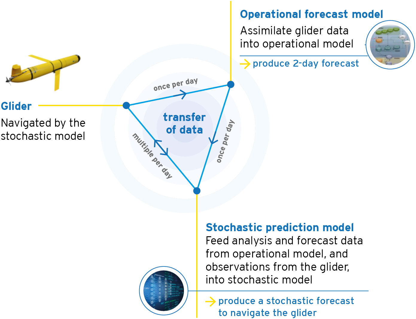
Figure 1 Schematic showing the integrated observing and forecasting system.

FIGURE 2

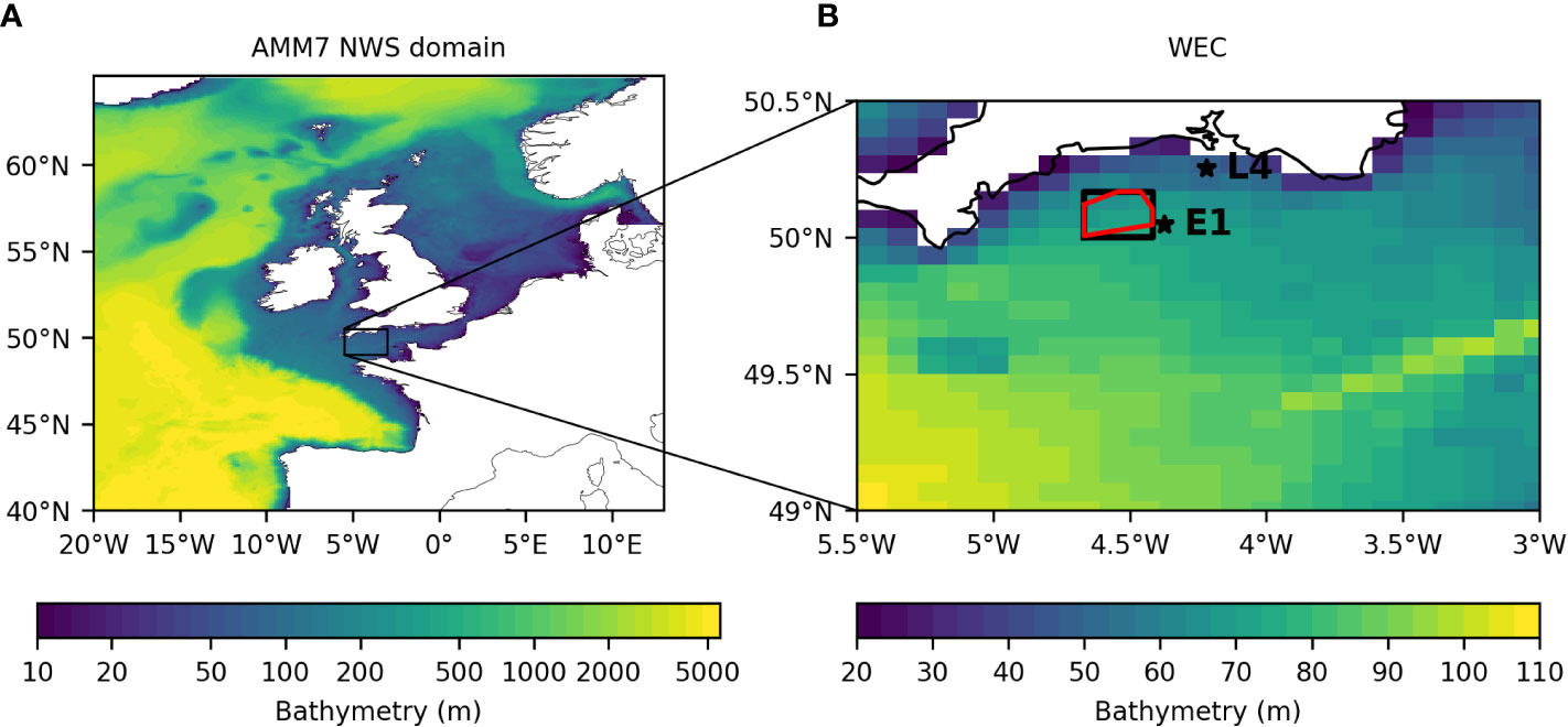
Figure 2 (A) AMM7 model domain and (B) close-up on the WEC, colored by the model bathymetry. In (B), the solid black box shows the area for which the stochastic prediction model produced chl-a forecasts. The red polygon shows the region in which the glider was allowed to travel and in which waypoints could be calculated. The stars show the location of the E1 and L4 time series stations.

2.1 Ocean glider

This study used a Slocum Glider (Teledyne Webb Research, Falmouth, USA) named Frazil (unit 438) from the Marine Autonomous and Robotic Systems facility at the National Oceanography Centre, UK (https://mars.noc.ac.uk). Slocum Gliders are AUVs that are propelled forwards in an up-down, “saw-tooth” profiling mode by controlling their buoyancy (Schofield et al., 2007). These mobile platforms are programmed to travel to prescribed locations (waypoints), with shallow water models typically sampling up to 200 m depth across coastal and shelf seas. Such missions enable the measurement of hydrographic and biogeochemical parameters with relatively little cost and power consumption (Testor et al., 2019).

Glider 438 was equipped with a Sea-Bird SBE42 conductivity, temperature, and depth (CTD) sensor to measure temperature, salinity and pressure (accuracy ±0.1%), an Aanderaa 4831 oxygen optode to measure dissolved oxygen concentration (O₂) (precision 0.2 μmol kg^-1, accuracy ±5%), a WETLabs triplet “puck” (with optical wavelengths optimized for chlorophyll-a (chl-a), colored dissolved organic matter, and backscatter fluorescence), and a Sea-Bird photosynthetically active radiation sensor.

Glider 438 was deployed by the Plymouth Marine Laboratory (PML) research vessel RV Plymouth Quest on 22 March 2021 at 50.042°N, -4.3712°W, and recovered on 8 June 2021 at 50.074°N, -4.4761°W. The glider moved through the water column with a nominal horizontal speed of 1.2 km h^-1, varying from 0.5 to 1.5 km h^-1, and an ascent/descent angle of 26°. Inflection points were set to 5 m from the surface and 5 m from the seabed with each yo-yo profile taking approximately 20 min. Every 90 min between 07:00 and 22:00 UTC the glider surfaced, relayed its latest real-time observations to the British Oceanographic Data Centre (BODC, https://www.bodc.ac.uk), and was able to receive new waypoints to direct the next part of the glider mission trajectory (see Section 2.4). Observations were made every 10 seconds.

The glider operation was constrained to the region of the WEC shown by the red polygon in Figure 2, approximately 18 km by 19 km, to minimize the risk of collision with heavy regional shipping and fishing traffic. The glider’s trajectory was guided by waypoints provided by a stochastic prediction model (see Section 2.4). The waypoints were provided automatically to a human pilot, who manually relayed them to the glider via satellite communication during regular surface intervals. While it was feasible to automate this relaying process direct to the glider machine-to-machine, regulatory requirements mandated that human control and oversight of the glider was required, to avoid collisions with ships in the busy WEC area. This restriction is discussed further in Section 4.

A subset of variables collected by the glider was transmitted via satellite communications on each surfacing interval and made publicly available online in NetCDF and png format by BODC, typically within 150 min of the glider surfacing. Users needed to perform their own near-real time (NRT) quality control (QC) and processing of these data, as detailed in Sections 2.3 and 2.4.

Following recovery, the complete dataset collected by the glider, commonly referred to as delayed mode (DM) data, underwent separate QC protocols. It was noted on recovery and in the quality of data collected that glider 438 had substantial biofouling, resulting in some data from 9 May 2021 onwards being deemed of insufficient quality for scientific use. This particularly affected salinity and O₂ measurements, as detailed in Section 3.1.

Coincident with the deployment on 22 March 2021, PML conducted CTD profiles from the RV Plymouth Quest at station E1 (Figure 2), measuring temperature, salinity, photosynthetically active radiation, fluorescence, and O₂. A CTD profile was conducted near the glider (0.75 km away) soon after deployment, enabling glider sensors (temperature, salinity, O₂) to be calibrated against CTD profile data and associated discrete water samples collected within 30 min and 0.75 km of glider deployment. Additional routine PML CTDs were conducted throughout the glider mission, but were considered unsuitable for glider calibration purposes, as they were too far from the glider location given the large regional horizontal gradients.

Increased seasonal solar heating at the end of May prompted an increase in surface mixed layer water temperature (>14°C) and vertical density stratification. Such conditions presented processing requirements to account for thermal inertia in the glider conductivity cell, which can potentially lead to errors in deriving salinity from the glider CTD data (Garau et al., 2011). Biofouling further reduced the thermal “connectivity” of the glider sensors with the surrounding seawater, increasing the thermal inertia effects and reducing data quality. Thermal inertia corrections (Garau et al., 2011) were applied to the DM data. Where such corrections did not significantly improve salinity data quality, by reducing the difference between consecutive ascending and descending profiles, the DM salinity data were deemed irrecoverable. This was most relevant to data collected towards the end of the deployment when biofouling had a clear and dramatic impact on data quality.

Compared with other oxygen optodes, the AA4831 has been documented by various scientific studies as being extremely stable with low detectable drift (<0.5% yr^-1) and high precision (<0.2 μmol kg^-1) (Champenois and Borges, 2012). However, a downside with the AA4831 oxygen optode is a potentially severe time response lag across strong O₂ gradients. O₂ data were therefore corrected where possible for optode membrane lag following Bittig et al. (2014). The previously mentioned biofouling in the latter stages of deployment prevented cross-calibration with RV Plymouth Quest CTD data collected prior to glider recovery, so O₂ optode drift could not be calculated. The manufacturer’s quoted downward drift value of 0.001% d^-1 was therefore used for O₂, which has been shown to be suitable in a similar coastal sea environment (Williams et al., 2022).

No calibration of fluorescence against other in situ data was performed during the experiment, so default factory calibrations were used to estimate total chl-a. Fluorescence calibration is discussed in more detail in Section 4. Proposed corrections for fluorescence quenching (Xing et al., 2012), which impacts the estimation of chl-a during the daytime, were not applied. Apart from near the beginning of the experiment, as detailed in the following sections, this study just used the nighttime chl-a data to avoid this issue.

2.2 Operational forecasting system

The Met Office runs two operational ocean forecasting systems for the NWS, delivering products to the Copernicus Marine Environment Monitoring Service (CMEMS), which are freely accessible for public use (Le Traon et al., 2019). A coupled physics-waves system is run on the ~1.5 km resolution Atlantic Margin Model (AMM15) domain (Tonani et al., 2019), and a physics-biogeochemistry system on the ~7 km resolution AMM7 domain (Edwards et al., 2012; McEwan et al., 2021). The AMM7 domain and its bathymetry is shown in Figure 2. The systems form part of the Forecasting Ocean Assimilation Model (FOAM) suite (Blockley et al., 2014), and at the time of the experiment the versions in operation were FOAM-AMM15 v2 and FOAM-AMM7 v11. Hereafter, these will be referred to as AMM15-OPER and AMM7-OPER, respectively.

The ocean physics model used is v3.6 of the Nucleus for European Modelling of the Ocean (NEMO). AMM7-OPER uses the CO6.2 configuration, which is a development of the CO5 configuration described by O'Dea et al. (2017). AMM15-OPER uses the CO8 configuration, similar to that described by Graham et al. (2018). Details of the physics atmospheric, river, and boundary forcing are given by Tonani et al. (2019).

The biogeochemistry model used is v19.04 of the European Regional Seas Ecosystem Model (ERSEM), a development of the v15.06 configuration described by Butenschön et al. (2016). ERSEM models the biogeochemistry and lower trophic levels of the pelagic and benthic ecosystem (Baretta et al., 1995; Blackford, 1997), including four phytoplankton types, three zooplankton types, and heterotrophic bacteria. ERSEM uses variable stoichiometry, representing biomass in carbon, phosphorus, and nitrogen constituents and, for diatoms, silicon. ERSEM is coupled to NEMO using the Framework for Aquatic Biogeochemical Models (FABM) (Bruggeman and Bolding, 2014). The coupling is one-way, so the physics affects the biogeochemistry but not vice versa. Details of the biogeochemical atmospheric, river and boundary forcing are given by McEwan et al. (2021).

AMM15-OPER and AMM7-OPER both assimilate observations using a 3D-Var configuration of NEMOVAR (Mogensen et al., 2009; Mogensen et al., 2012; Waters et al., 2015). Physics observations assimilated are satellite and in situ sea surface temperature (SST), in situ temperature and salinity profiles, and satellite sea level anomaly, as detailed by King et al. (2018) and Tonani et al. (2019). Chl-a derived from satellite ocean color is assimilated into the biogeochemical component of AMM7-OPER (McEwan et al., 2021), using the method described by Skákala et al. (2018; 2021). Prior to assimilation, a background check is performed on the ocean color data (Ford et al., 2012). This compares the observations to the latest model background field, and rejects observations with too large a departure from the background, given estimates of the observation and background error standard deviations (Ingleby and Huddleston, 2007). The remaining observations are then median averaged to a radius of 7 km (Ford et al., 2012; Skákala et al., 2018).

The forecasting systems are run daily. In each cycle, analyses are produced for the preceding two days, to maximise the number of observations available for assimilation. Due to the availability time of ocean color data from CMEMS, ocean color observations are only assimilated into the first day’s analysis, referred to as the “best estimate” of the ocean state. Following the two analysis days, a six-day forecast is produced.

Postprocessing is then performed to convert from the terrain-following coordinates of the native model grid (Siddorn and Furner, 2013) to a standard grid with geopotential levels (Tonani et al., 2019), and data uploaded to CMEMS. Daily mean and hourly instantaneous fields are available from AMM15-OPER, and daily mean fields from AMM7-OPER. Products are typically updated at 12:00 UTC.

2.3 Pseudo-operational forecasting system

For the duration of the experiment, an alternative version of AMM7-OPER was run pseudo-operationally. This was essentially a copy of AMM7-OPER, modified to assimilate observations from the glider, and provide bespoke outputs. The system will be referred to as AMM7-CAMPUS.

AMM7-CAMPUS assimilated chl-a and O₂ observations from the glider, into both analysis days, using the method described by Skákala et al. (2021). Assimilating glider chl-a also required a modification to the ocean color assimilation, as discussed by Ford (2021) and Skákala et al. (2021). In AMM7-OPER, 2D chl-a increments are calculated by NEMOVAR, and applied equally through the mixed layer. In AMM7-CAMPUS, 3D chl-a increments were calculated by NEMOVAR, using flow-dependent vertical correlation length scales as detailed by King et al. (2018) and Skákala et al. (2021). To test the impact of this modification, a further system was run assimilating ocean color with 3D increments from NEMOVAR, but not assimilating observations from the glider. This showed minimal differences from AMM7-OPER in the WEC, giving confidence that any differences in results between AMM7-OPER and AMM7-CAMPUS can be fully attributed to assimilating the glider observations. Temperature and salinity observations from the glider were not assimilated, in order to preserve operational observation preprocessing procedures, and because the impact on biogeochemical forecasts has previously been shown to be small (Skákala et al., 2021).

Prior to assimilation each day, AMM7-CAMPUS downloaded the latest glider observations from BODC, and applied some preprocessing. This consisted of a file format conversion, O₂ unit conversion, log-transformation of chl-a, and median averaging. Log-transforming chl-a is required by the assimilation (Skákala et al., 2021), as it makes the error distribution more Gaussian (Campbell, 1995). Median averaging is common practice in data assimilation (Skákala et al., 2021), to avoid assimilating many high-resolution observations representing small-scale processes the model cannot resolve, which can lead to instabilities in the model. Initially, the median observation value in each model grid cell between 00:00-23:59 UTC each day was used. From 8 April 2021, the change was made to reject glider chl-a data between 06:00-20:00 UTC, as daytime data may be affected by fluorescence quenching (Xing et al., 2012). Rather than a single median daily value being assimilated per grid cell, two values were now assimilated (if observations available): the median observation between 00:00-06:00 UTC, and the median observation between 20:00-23:59 UTC.

For use by the stochastic prediction model, hourly mean chl-a was output on the native model grid, for a region in the WEC around where the glider was being operated, covering an area surrounding the black box in Figure 2. Initially, this region covered 4.72°W to 4.28°W, 49.90°N to 50.30°N. From 6 April 2021, the region was enlarged to 4.83°W to 4.17°W, 49.90°N to 50.30°N. These outputs were automatically placed on an FTP server, and most days were updated between 11:00-12:00 UTC.

While the glider was recovered on 8 June 2021, AMM7-CAMPUS was kept running until 24 June 2021, to assess the lasting impact of assimilating the glider data.

2.4 Stochastic prediction model

A stochastic prediction model was used to predict chl-a at high resolution and calculate waypoints for the glider. The model will be fully described and validated in a separate paper by Menon et al. (in prep.), and will hereafter be referred to as STOCHASTIC. It uses the integrated nested Laplace approximation (INLA) (Rue et al., 2009; Lindgren et al., 2011) to approximate Bayesian inference, which can be downloaded from https://www.r-inla.org. Chl-a was modelled using the stochastic partial differential equation approach inferred using the INLA method. Given observations of chl-a at different locations the unknown 2D chl-a was considered as a Gaussian field. The Matérn covariance function was used to model spatial autocorrelation and uncertainty. The correlation among the cells in the modelling can often contribute to computational complexity. From the analysis of several potential influencing variables such as radiation, mixed layer depth, wind stress, chl-a, current velocity, nitrate, O₂, phosphate, temperature, and turbidity, it was found that only temperature and chl-a had direct influence contributing to the prediction of chl-a. Therefore, chl-a and SST inputs were used.

STOCHASTIC took as inputs the latest glider chl-a observations, hourly-resolution analyses and forecasts of SST from AMM15-OPER, and hourly-resolution analyses and forecasts of chl-a from AMM7-CAMPUS. In the event of any delay in the production of AMM7-CAMPUS forecasts due to the research nature of the system, STOCHASTIC would use daily-resolution chl-a data from AMM7-OPER. A subset of AMM7-CAMPUS was passed to STOCHASTIC, as detailed in Section 2.3, as information was only required for the region in which the glider was permitted to travel, plus the surrounding area in case the glider left the permitted region. As discussed in Section 3.1, on 2 April 2021 the glider drifted outside this area, so from 6 April 2021 a larger area was passed, as detailed in Section 2.3.

Each time STOCHASTIC was run, it was trained using the glider chl-a and model chl-a and temperature analyses for the previous 72 hours (prior to 5 May 2021) or 120 hours (5 May 2021 onwards), and then used to produce a 24-hour chl-a forecast at 4-hourly resolution by combining the input forecast data with random effects. The chl-a forecast was produced on a 0.0014° longitude by 0.0009° latitude (approximately 100 m by 100 m) resolution grid covering the region in which the glider was permitted to travel (Figure 2). The forecast was 2D at a depth of 10 m until 14 April 2021, after which it was calculated at the mean depth of maximum chl-a from the glider observations, up to a maximum of 30 m. During the training stage, the model chl-a and temperature analyses were interpolated onto the location of the glider chl-a observations in spacetime, using quadrilinear interpolation, which is similar to that used by Dai and Sweetman (2016). During the forecast stage, the model chl-a and temperature analyses were interpolated onto the forecast grid, using quadrilinear interpolation.

Prior to 14 April 2021, all glider chl-a observations in the training period were used. After this date, only nighttime data were used due to potential fluorescence quenching as discussed in Sections 2.1 and 2.3. This reduction in the number of data points per day led to the later increase in the length of the training period from 72 to 120 hours to compensate.

From the forecast a set of six waypoints was calculated, one at each 4-hourly interval of the 24-hour forecast, giving a series of locations to direct the glider towards over the next 24 hours. These were calculated as the locations where the maximum chl-a in the region was most likely to be, based on the predicted mean value and variance of chl-a on the forecast grid. Movement constraints were also accounted for. The waypoints were then communicated via email to the glider pilot in a fully automated process using a Linux bash script. Following an initial validation period, these waypoints were used to steer the glider from 26 March 2021 onwards.

After the glider deployment was completed, a set of offline sensitivity experiments was performed. For a selection of times during May 2021, STOCHASTIC was rerun three times using different model chl-a inputs. First, using AMM7-CAMPUS chl-a, as was done during the deployment. Second, using AMM7-OPER chl-a, which did not assimilate the glider data. Third, not using any model chl-a, only the glider chl-a. In each case the initial glider position was that during the deployment, so these experiments give a snapshot of the sensitivity of predictions and waypoints to the input data sources, as detailed in Section 3.4.

2.5 Other observations

For validation and intercomparison, this study also used chl-a derived from satellite ocean color, and in situ observations from the Western Channel Observatory (Smyth et al., 2010; Smyth et al., 2015).

Ocean color data were taken from the CMEMS North Atlantic NRT product (https://doi.org/10.48670/moi-00284), which provides level 3 daily merged chl-a from the MODIS-Aqua, VIIRS, and OLCI-3A sensors. This is the same ocean color product as assimilated by AMM7-OPER and AMM7-CAMPUS. During the experiment, single-sensor ocean color data for the WEC was emailed daily to team members by NEODAAS (https://www.neodaas.ac.uk/), for monitoring purposes.

In situ chl-a observations from the E1 and L4 stations (Smyth et al., 2010; Smyth et al., 2015) in the WEC (Figure 2) were used for validating the differences between AMM7-OPER and AMM7-CAMPUS. These stations form part of the Western Channel Observatory, and physical and biogeochemical parameters are sampled approximately weekly by PML.

3 Results

The results are split into four subsections, linked to the objectives of the study detailed in Section 1. The first subsection details the path taken by the glider, the glider observations, and differences between the NRT and DM data. The second subsection assesses differences between AMM7-OPER and AMM7-CAMPUS results due to assimilating the glider data. The third subsection intercompares chl-a estimates from the glider, ocean color, AMM7-OPER, AMM7-CAMPUS, and STOCHASTIC. The fourth subsection assesses the sensitivity of STOCHASTIC to different inputs.

3.1 Glider observations

The course taken by the glider is shown in Figure 3. The glider covered most of the region of interest during the experiment, though never sampled the most northern latitudes. Its position was focused on different areas in different periods, as directed by STOCHASTIC.

FIGURE 3

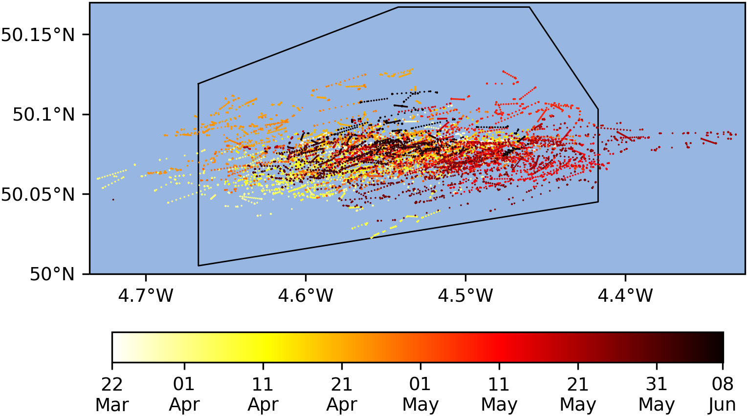
Figure 3 Reported surface positions of the glider (colored dots). The black polygon shows the region to which the glider waypoints were restricted.

The glider was constrained to remain within the area marked in Figure 3, and all waypoints calculated by STOCHASTIC were similarly constrained to this area as required. Occasionally though, strong east-west tidal currents carried the glider outside of the intended control area. One such breach occurred on 2 April 2021 when the glider drifted beyond the region being supplied to STOCHASTIC by AMM7-CAMPUS, causing STOCHASTIC to fail. To compensate, STOCHASTIC was temporarily set to use AMM7-OPER data for 72 hours, and the area supplied from AMM7-CAMPUS was later expanded, as detailed in Sections 2.3 and 2.4. In future, information on currents could be added to the movement constraints considered by STOCHASTIC, as discussed in Section 4.

Plots along the glider transect are shown in Figure 4 for temperature, salinity, chl-a, and O₂, from the NRT and DM glider data. One of the key objectives of the experiment was to capture details of the spring bloom, and bloom events were observed in April (Figures 4E, F). An initial near-surface bloom was observed on 20-21 April 2021, followed by a larger bloom throughout the water column on 25-27 April 2021. This was associated with sudden changes in temperature and salinity (Figures 4A–D), related to precipitation and wind conditions (not shown). An imprint could also be seen on O₂ (Figures 4G, H), driven by changes in solubility.

FIGURE 4

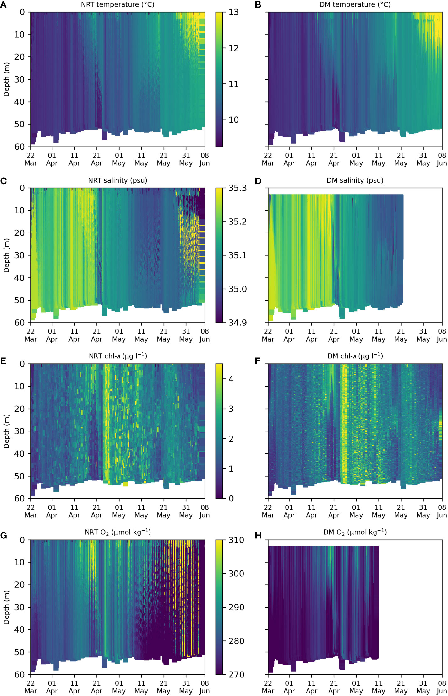
Figure 4 Plots along the glider transect for different variables, from the NRT glider data (left column) and DM quality-controlled glider data (right column). (A) NRT temperature, (B) DM temperature, (C) NRT salinity, (D) DM salinity, (E) NRT chl-a, (F) DM chl-a, (G) NRT O₂, (H) DM O₂.

From late May the water column began to stratify (Figures 4A, B), and at the very end of the experiment a corresponding deep chlorophyll maximum (DCM) appeared to be forming below the base of the mixed layer (Figure 4F).

As mentioned in Section 2.1, significant biofouling occurred, particularly affecting the O₂ and salinity measurements. This resulted in extremely noisy values in the NRT data for these variables towards the end of the experiment (Figures 4C, G), and the removal of these from the DM data (Figures 4D, H). Near-surface values from these variables were also removed from the DM data, as these depths were not properly resolved. Additional biofouling appeared to occur at the very end of the experiment for all sensors, but this could be corrected for in the DM data.

A further issue with the NRT O₂ data was the apparently unnaturally high magnitude of the observed values. It was discovered after deployment that the O₂ sensor had been default calibrated for freshwater rather than seawater, providing apparent O₂ values that were significantly higher than expected. An offline correction was applied during the experiment based on the observed salinity, and these corrected values are shown in Figure 4G, but further correction was required during DM processing (Figure 4H). The erroneous NRT O₂ data were assimilated into AMM7-CAMPUS for the whole duration of the experiment, and this adversely affected model O₂ values (not shown). Fortunately for the purposes of this experiment, the impact on other model variables, including chl-a, was negligible. This is because there is only very weak feedback from O₂ to ecosystem variables in ERSEM (Butenschön et al., 2016; Skákala et al., 2021).

In both the NRT and DM data, chl-a values are highly variable throughout the water column (Figures 4E, F). This is possibly due to the presence of phaeocystis colonies, which have been observed to cause spikes in vertical profiles of fluorescence (Tarran and Bruun, 2015).

3.2 Impact of glider data assimilation on forecast model

To assess the impact of assimilating the glider data on AMM7-CAMPUS, plots of chl-a are shown in Figure 5. These show the assimilated satellite and glider data, and the AMM7-OPER and AMM7-CAMPUS best estimate and six-day forecasts. Satellite chl-a (Figure 5A) within the glider region (after background check and median averaging) is plotted to the depth of the AMM7-CAMPUS mixed layer, using the definition of Kara et al. (2000) as is used in calculating the vertical correlation length scales in the data assimilation (King et al., 2018). Glider chl-a (Figure 5B) is equivalent to that plotted in Figure 4E, but after median averaging. The model chl-a (Figures 5C–F) is the mean over the nine AMM7 grid squares covering the glider region, on the standard geopotential levels provided to CMEMS (Tonani et al., 2019), and includes a period after the glider deployment ended, as described in Section 2.3.

FIGURE 5

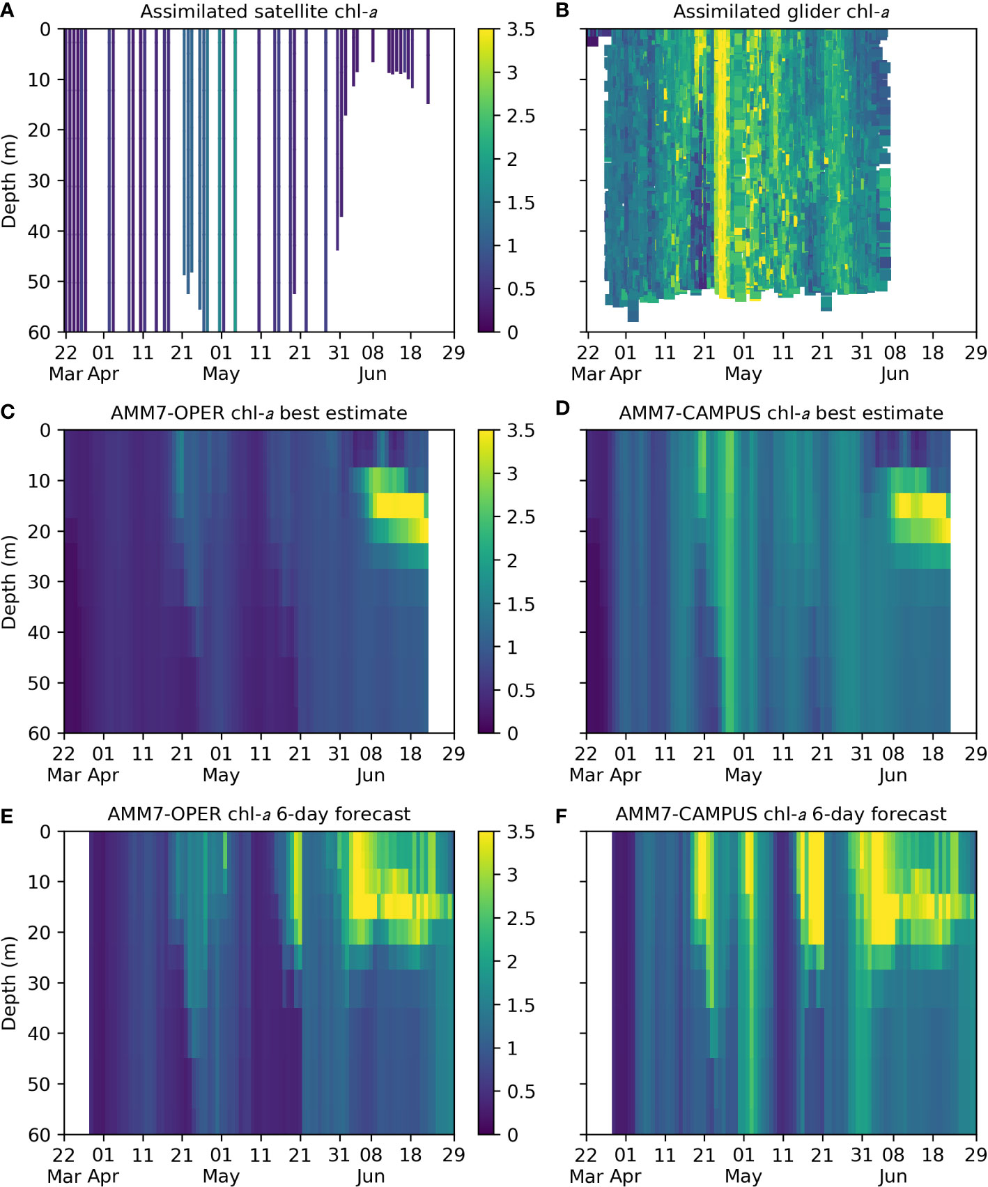
Figure 5 Plots of chl-a (mg m^-3) from (A) assimilated preprocessed satellite data within the glider region plotted to the AMM7-CAMPUS mixed layer depth, (B) assimilated preprocessed glider data, (C) AMM7-OPER best estimate averaged over the glider region, (D) AMM7-CAMPUS best estimate averaged over the glider region, (E) AMM7-OPER six-day forecast averaged over the glider region, (F) AMM7-CAMPUS six-day forecast averaged over the glider region.

Glider chl-a values were typically higher than satellite chl-a, but with similar temporal variability. This difference carried through to the AMM7-CAMPUS best estimate, which assimilated both data sources, compared with AMM7-OPER which only assimilated the satellite data. Both models reproduced the observed blooms in late April, but these were much more prominent in AMM7-CAMPUS, especially the larger bloom in the glider data. Throughout the glider deployment, the water column was mostly well-mixed in the glider and model data, apart from some dates in mid-April and mid-May. Around the end of the deployment, near-surface chl-a reduced in both AMM7-OPER and AMM7-CAMPUS, and a DCM formed, as started to be seen in the glider data (Figure 4F). This DCM persisted until the end of the model run.

The initial spring bloom activity around 20 April 2021 appears to have been well forecast six days out by both AMM7-OPER and AMM7-CAMPUS, with increased magnitude in AMM7-CAMPUS. The larger bloom seen in the glider observations a few days later was missing from the AMM7-OPER forecasts, and in AMM7-CAMPUS it was forecast six days too late, suggesting that it was merely persisted from the analysis after those observations were assimilated. The formation of a DCM at the end of the glider deployment was also present in both sets of forecasts. As with the best estimate, chl-a values were typically higher in the AMM7-CAMPUS forecasts than in AMM7-OPER. Correspondingly, depth-integrated net primary production was 20-50% higher in AMM7-CAMPUS (not shown).

To assess the wider spatial impact of assimilating the glider data, the mean absolute difference in surface chl-a between AMM7-OPER and AMM7-CAMPUS in the WEC during the glider deployment is plotted in Figure 6. For the best estimate (Figure 6A) the biggest differences are found in the immediate vicinity of the glider, with smaller differences locally in the WEC. In part, this limited spatial impact will be due to the ocean color assimilation also acting to constrain chl-a in both systems. In the six-day forecasts (Figure 6B), the biggest differences remain in the vicinity of the glider and immediately to the east, and are smaller in magnitude. The extent of the spatial differences across the WEC is much larger, however.

FIGURE 6

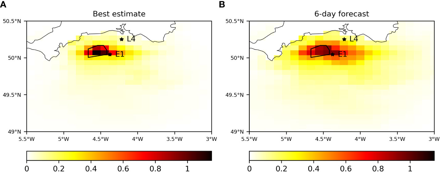
Figure 6 Mean absolute difference in surface chl-a (mg m^-3) between AMM7-CAMPUS and AMM7-OPER during the glider deployment, computed for (A) the first analysis day and (B) the six-day forecast. The black polygon shows the region in which the glider was permitted to travel. The stars show the location of the E1 and L4 time series stations.

To validate against independent in situ data, AMM7-OPER and AMM7-CAMPUS chl-a values have been compared with fluorescence profiles at station E1, situated just outside the glider region (Figure 2). Profiles at E1 were conducted on four dates during the glider deployment: 7 April 2021, 21 April 2021, 26 May 2021, and 8 June 2021. The observations were at very high vertical resolution (0.25 m) and very noisy. Therefore, a 2.5 m rolling mean was applied to each profile, before a cubic spline interpolation was performed to map the observations onto the geopotential levels of the CMEMS products. This gave a total of 40 observation points to compare against across the four dates. Model values were then linearly interpolated in the horizontal to the E1 location to create model-observation matchups. Validation was performed using robust statistics, due to the lognormal distribution of chl-a (Campbell, 1995). Following McEwan et al. (2021), the metrics used were median bias, median absolute difference, and Spearman rank correlation coefficient. Validation results for the best estimate and six-day forecasts from AMM7-OPER and AMM7-CAMPUS are shown in Table 1. All metrics were improved in AMM7-CAMPUS compared with AMM7-OPER, for both analysis and forecast. This provides confidence that assimilating the glider data improved model results.

TABLE 1

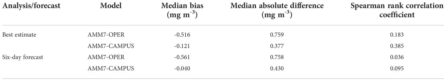
Table 1 Validation statistics for AMM7-OPER and AMM7-CAMPUS chl-a against E1 data.

At station L4, situated further from the glider region (Figure 2), profiles were conducted on 11 dates during the glider deployment. The observations and models were treated in the same way as for the E1 data, giving a total of 88 model-observation matchups. Validation results for the best estimate and six-day forecasts from AMM7-OPER and AMM7-CAMPUS are shown in Table 2. The differences between the two forecasting systems were smaller than at E1, consistent with the spatial extent of differences shown in Figure 6. For the best estimate, median absolute difference was slightly improved in AMM7-CAMPUS compared with AMM7-OPER, while median bias and Spearman rank correlation coefficient were slightly degraded. For the six-day forecasts all metrics were improved in AMM7-CAMPUS, but by a smaller margin than at E1.

TABLE 2

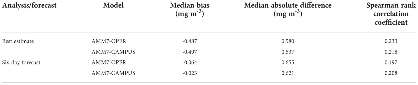
Table 2 Validation statistics for AMM7-OPER and AMM7-CAMPUS chl-a against L4 data.

3.3 Intercomparison of models and observations

In this subsection, the temporal and spatial representation of chl-a in the glider region is compared between the different observation and model products. It should be noted that none of the data sources are independent, and all have uncertainties, so this is an intercomparison rather than validation.

Figure 7 shows a time series of near-surface chl-a in the glider region from each data source. Shown are the nighttime glider observations in the upper 10 m, the daily mean of these observations, ocean color observations, hourly AMM7-OPER surface best estimate, hourly AMM7-CAMPUS surface best estimate, and four-hour predictions from STOCHASTIC. The glider observations show extremely large sub-daily variability, possibly due to the presence of phaeocystis colonies as discussed in Section 3.1, with less variability in the daily mean. As seen in Figure 4, the highest chl-a was a bloom in late April. The ocean color observations were all smaller than the glider daily mean, and mostly outside the range of variability in the nighttime glider data. The ocean color satellites are heliocentric, sampling at approximately local noon, when glider data have been excluded as they may be affected by fluorescence quenching. AMM7-OPER closely matched the ocean color data, except in June, while AMM7-CAMPUS was usually between the ocean color and glider observations in magnitude. STOCHASTIC was usually close to the glider daily mean. After the glider deployment ended, surface chl-a in the region in AMM7-OPER and AMM7-CAMPUS converged within a week, as soon as ocean color data were available and the analyses were being constrained by the same observations.

FIGURE 7

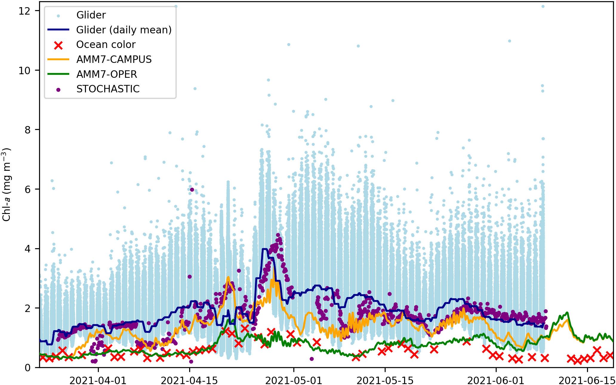
Figure 7 Time series of near-surface chl-a in the glider region from the nighttime glider observations, ocean color, AMM7-CAMPUS best estimate, AMM7-OPER best estimate, and STOCHASTIC four-hour predictions.

The spatial distribution of chl-a in the region in each data source is shown for two dates, one during each of the bloom events, in Figures 8, 9.

FIGURE 8

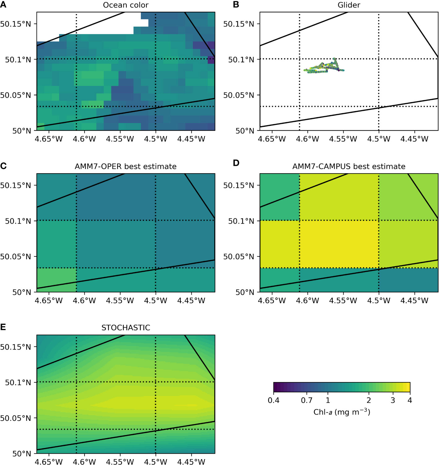
Figure 8 Chl-a in the glider region on 20 April 2021, from (A) ocean color (white area is missing data due to cloud), (B) glider observations in the upper 10 m, (C) AMM7-OPER surface best estimate, (D) AMM7-CAMPUS surface best estimate, (E) STOCHASTIC, first four-hour prediction of the day. The solid black lines denote the region the glider was constrained to stay within. The dotted black lines denote the AMM7 model grid. Note the use of a log color scale.

FIGURE 9

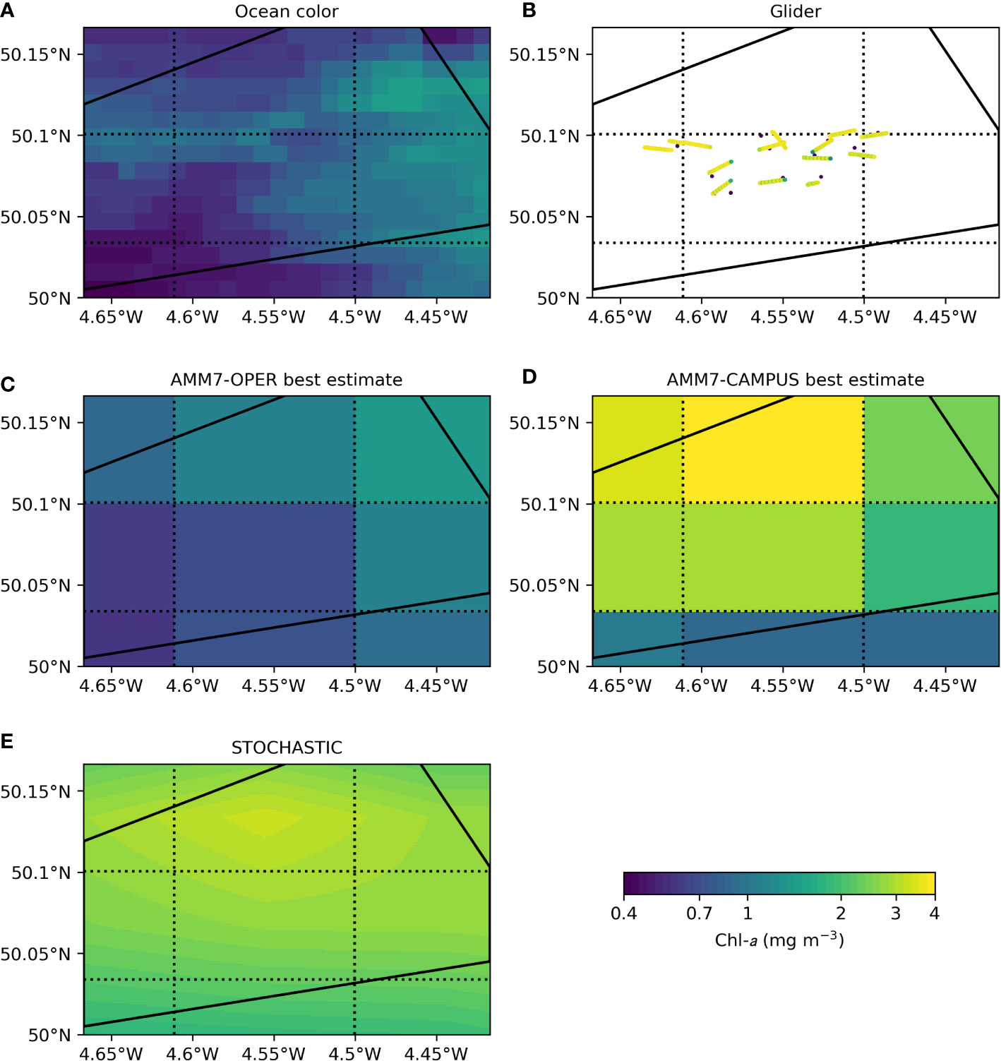
Figure 9 Chl-a in the glider region on 26 April 2021, from (A) ocean color, (B) glider observations in the upper 10 m, (C) AMM7-OPER surface best estimate, (D) AMM7-CAMPUS surface best estimate, (E) STOCHASTIC, first four-hour prediction of the day. The solid black lines denote the region the glider was constrained to stay within. The dotted black lines denote the AMM7 model grid. Note the use of a log color scale.

Figure 8 shows 20 April 2021, during the first chl-a peak seen in Figures 4, 7. The ocean color data (Figure 8A) showed a certain amount of spatial variability, with the highest chl-a just to the west of the center of the region. Significantly, this broadly matches where the glider was sampling that day (Figure 8B). AMM7-OPER (Figure 8C) and AMM7-CAMPUS (Figure 8D) lack the spatial resolution to fully resolve the region, but did show some spatial variability. AMM7-OPER had higher chl-a in the south and west than the north and east, in broad agreement with the ocean color. AMM7-CAMPUS had the highest chl-a in the center of the region, reflecting the location of the glider data, which were higher in magnitude than the ocean color. STOCHASTIC (Figure 8E) had a zonal line of high chl-a across the lower center of the region, with lowest chl-a in the corners, broadly reflecting AMM7-CAMPUS.

Figure 9 shows 26 April 2021, during the second chl-a peak seen in Figures 4, 7. In those plots, a peak was seen in the glider data but not the ocean color. This is also seen in Figure 9. The ocean color (Figure 9A) had low chl-a across the region, slightly higher in the east. The glider (Figure 9B) sampled throughout the center of the region, with much higher magnitudes. AMM7-OPER (Figure 9C) reflected the ocean color data. AMM7-CAMPUS (Figure 9D) had highest chl-a north of the center, and lowest chl-a to the south, beyond the area where the glider could sample. STOCHASTIC (Figure 9E) was broadly comparable to AMM7-CAMPUS, but more homogeneous. A critical aspect of using quadrilinear interpolation for the model inputs to STOCHASTIC is that no additional new information is generated at the data point locations. The data values are only being smoothed between data points. However, by also including the glider chl-a observations in the model, the forecasts are affected by the assimilation of the observations in the vicinity of these locations, as can be seen in Figures 8, 9. This is most useful in improving the path planning, as well as reducing the level of uncertainty.

During the experiment, there was full coverage of the glider region by ocean color on 16 days. To compare the glider’s sampling positions with the location of maximum chl-a estimated from ocean color data, for each of these 16 days the ocean color chl-a is shown in Figure 10, overlaid with the glider positions during that day. The ocean color chl-a is not the “truth”, but is an alternative observational estimate of the spatial variability of chl-a. While ocean color data were assimilated by AMM7-CAMPUS, which was used in navigating the glider, the observations for a given day had not yet been assimilated at that point so can be considered semi-independent.

FIGURE 10

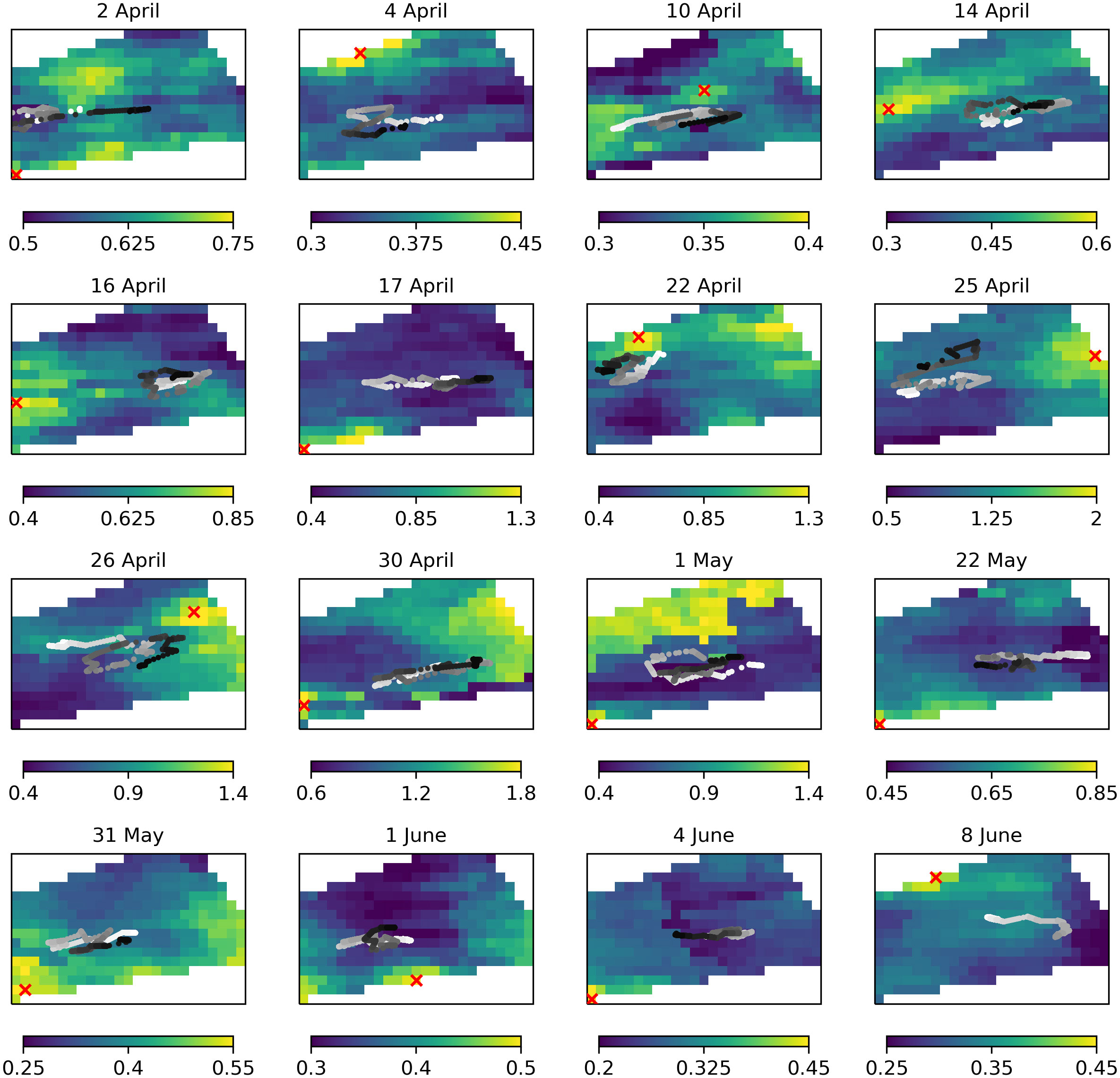
Figure 10 For each day with complete ocean color coverage, maps of chl-a (mg m^-3) from ocean color overlaid with the glider positions that day (grey dots, getting darker from white to black between 00:00 and 23:59) and position of maximum chl-a estimated from ocean color (red crosses).

On none of the days did the glider sampling coincide with the ocean color pixel of maximum chl-a, though on many occasions this occurred on the very border of where the glider could be sent. Even if the glider did not sample the highest chl-a estimated from ocean color, it did often – though not always – sample in the vicinity of patches of higher rather than lower chl-a. Qualitatively, the impression is also given from Figure 10 of the glider successfully chasing around the area of highest chl-a, even if it did not manage to reach it. The comparison is complicated by the merging of different ocean color sensors, which may not always agree, in the ocean color product used. For instance, the sharp gradient seen on 1 May 2021 (Figure 10) represents the edge of a satellite swath. Furthermore, the ocean color data provides a snapshot in time, while the glider was iteratively directed towards different potential chl-a maxima throughout each day, with strong tidal currents continually advecting any phytoplankton.

3.4 Sensitivity of stochastic prediction model to inputs

For select times in May 2021, STOCHASTIC was rerun using different inputs, as described in Section 2.4, to assess the sensitivity of the calculated waypoints to the use of model data. A representative example is shown in Figure 11, showing the 24-hour chl-a predictions for 20:05 on 14 May 2021, using AMM7-CAMPUS chl-a (Figure 11A), AMM7-OPER chl-a (Figure 11B), and only glider chl-a (Figure 11C). Overlaid are the set of 6 waypoints to which the glider would be successively directed based on the predictions, with 0 showing the starting location of the glider. When using AMM7-CAMPUS, as was done during the deployment, the highest chl-a was predicted to be in the current vicinity of the glider, and the glider was directed to stay around that location. If AMM7-OPER data were used instead, there was less variability in the predictions, with highest chl-a in the opposite corner of the domain outside of where the glider could be directed. The glider would instead be directed toward the centre of the domain. In the case where no model chl-a was provided the prediction was extremely homogeneous, and the glider would be directed to the northwest of its current location.

FIGURE 11

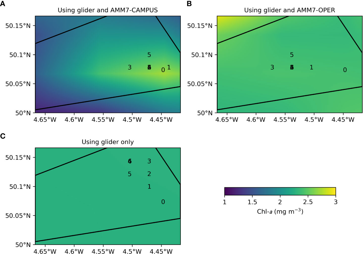
Figure 11 24-hour chl-a predictions for 20:05 on 14 May 2021 from STOCHASTIC using different model chl-a inputs: (A) glider and AMM7-CAMPUS, (B) glider and AMM7-OPER, (C) glider only. The black lines denote the region the glider was constrained to stay within.

4 Summary and discussion

This study has introduced and demonstrated, as a proof-of-concept, an automated and adaptive ocean observing system integrating an ocean glider with operational ocean model forecasts. The glider was deployed in the western English Channel (WEC) during the spring bloom period of 2021 and directed by waypoints autonomously provided by a stochastic prediction model. This combined the glider observations with forecasts from a numerical model, which in turn assimilated the glider observations and other data, to create high-resolution probabilistic predictions of chl-a. From these, a set of waypoints was calculated, to direct the glider to where a phytoplankton bloom was most likely to be found. Optimised adaptive sampling strategies were therefore provided via a continuous feedback loop from machine-to-machine. The glider successfully captured details of the spring bloom in the WEC at unprecedented temporal resolution. Furthermore, assimilating these observations appeared to have a positive impact on operational forecasts in the region, consistent with the previous work of Skákala et al. (2021), although the region of influence was limited and few independent observations were available for validation. When comparing the predicted bloom locations with ocean color data the results were ambiguous, perhaps due to the small study region and differences between remotely sensed and in situ chl-a measurements, as discussed below.

Traditionally, a glider is directed by a human based on scientific judgement, or set on a predefined course. The system trialled in this study offers an alternative and arguably improved method, where the locations of features of interest are predicted by models based on all available sources of information, and the glider is directed accordingly with no human decision being made other than oversight for safety. This has the potential to better ensure observations are made where they will be of most use and have the most impact. Cost savings are also likely by reducing the need for human input and potentially making efficiencies where multiple autonomous underwater vehicles (AUVs) are deployed, making a glider-based ocean observing system more affordable. Currently, in situ monitoring of coastal seas is sparse, and largely limited to static buoys and moorings, research vessel campaigns, and satellite data. Autonomous marine technologies such as the glider trialled present an affordable and scalable alternative or complementary framework that could significantly increase the density and effectiveness of coastal ocean observing networks.

Several challenges remain before such a system is ready for operational implementation. One relates to near-real time (NRT) versus delayed mode (DM) quality control (QC). Biofouling became a major issue in this study towards the end of the 11-week deployment. Unless solutions are found, biofouling will always be a concern in shallow, well-lit, productive waters such as the WEC that are typical of coastal and shelf seas. This will likely limit future glider missions to shorter durations. Automated QC would help with identifying when this is affecting data quality and could be used to flag the need for glider recovery and replacement. This study also shows that care and consideration need to be taken around calibration, to enable the maximum opportunities to cross calibrate with other available data sources throughout deployments. In this study, the DM O₂ values were significantly different to the NRT values after QC, leading to inaccurate results when used for monitoring and assimilation in NRT. Calibration of fluorescence and its translation to total chl-a biomass also remains a challenge for the observing community, in both NRT and DM mode, and is reflected in challenges faced in operational QC of Biogeochemical-Argo floats (Roemmich et al., 2019). A comparison and collaboration on QC methods between the glider and Biogeochemical-Argo communities may be desirable, for instance within the framework of the Ocean Best Practices System of the Intergovernmental Oceanographic Commission (Pearlman et al., 2019).

Similarly, differences between chl-a estimates derived from satellite ocean color and gliders pose challenges when assimilating both data types into operational models. Resolving differences in sampling frequency, coverage, and sensor optical frequency ranges presents issues, and even collocated satellite and in situ estimates can present significantly different values as they are not designed to measure the same volumes of water. Furthermore, this study only used nighttime glider data to avoid contamination due to fluorescence quenching, while ocean color sensors take measurements at approximately midday. This timing offset can lead to differences due to advection and changes in biological production. Very high-resolution variability in vertical profiles of fluorescence (Tarran and Bruun, 2015) can exacerbate these issues further. Some account of this is taken during the assimilation process, for instance through median averaging and assigning different errors to each observation type, but more work is required to develop this. Intercomparisons of models, ocean color, and bio-optical observations from Biogeochemical-Argo floats have been investigated (IOCCG, 2011; IOCCG, 2020), and such efforts should be extended to emerging autonomous monitoring systems. It would be possible to perform vicarious calibration to “correct” one set of observations based on the other, but this would need to be done carefully to avoid making inappropriate assumptions about the relative accuracy of each dataset. Furthermore, DM ocean color products can come with bias and uncertainty information provided (Jackson et al., 2017), allowing the ocean color data to be bias-corrected prior to assimilation (Ciavatta et al., 2016; Skákala et al., 2018). This information is not currently available for the NRT product assimilated operationally.

Scaling up the observing system to include multiple AUV platforms presents further challenges. In this study, a single glider was deployed, and restricted to a relatively small region. To provide wider geographic improvement to operational model forecasts, and provide more comprehensive monitoring, a much larger region would feasibly need to be covered by multiple AUVs. A more complex stochastic prediction model would therefore be required to consider, for example, that multiple AUVs are not sent to the same location, AUVs are only directed to locations they can reach in a reasonable time, and that moving one AUV doesn’t improve predictions in a small area to the detriment of the wider regional forecast. This would need to account for both the AUVs’ nominal speed and the ocean currents. The inability in this study to constrain a single glider to a control area due to regionally typical tidal currents highlights the complexity of controlling multiple autonomous platforms within the natural variability of coastal ocean currents and density structure. The relatively small size of the region, covered by only a few grid cells of the operational forecasting model, meant that spatial variability in the forecasts was limited. The interactions between the different data sources in a larger domain, and how this may impact the path planning, requires further investigation.

The stochastic prediction model used operational ocean forecasts as inputs, as well as the glider observations. The use of model as well as observation data adds a layer of complexity, especially when the glider data is also being assimilated. Whether a model was used, and whether it assimilated the glider data or not, was shown to significantly alter the results, suggesting this added complexity to be worthwhile. Care should be taken though not to introduce an inadvertent positive feedback loop, where biases between the glider observations and other data sources act to keep the glider in one small area, because all glider observations are systematically higher in magnitude than the other sources. This did not appear to be the case in this study, but was difficult to assess given the small area. A way to mitigate this risk might be through online bias correction, or weighting the different data sources based on estimates of their errors. A further issue is the relatively low spatial resolution of the model forecasts, especially given the limited study area over which the model could not fully resolve spatial gradients. Higher model resolution is ideally required, but this is computationally challenging and innovative solutions may be needed. Operational biogeochemical models can play a crucial role in monitoring and decision making (Fennel et al., 2019), but are not always used to their full potential (Hyder et al., 2015). Initiatives to promote such systems are to be supported (ETOOFS, 2022).

In this study, the stochastic prediction model aimed to direct the glider towards the maximum chl-a in the region, as a measure for the most likely location of a potentially harmful algal bloom. Other criteria could be used, and these might be more appropriate in other studies. For instance, an algorithm was also developed to follow a contour of a given variable, to allow the extent of a bloom or anomalous temperature spot to be mapped. The stochastic prediction model can also calculate the uncertainty in chl-a or another variable given the input data, and an alternative strategy could be to direct the glider to the location of the highest uncertainty. In deciding the appropriate strategy, there may be a tension between different applications. For monitoring bloom activity, tracking the maximum or a contour might be favoured. For improving model forecasts, sampling areas of highest uncertainty might be favoured.

With any glider deployment, pragmatic trade-offs are required between scientific interest, safety, and battery life. These become paramount in an automated system with more limited human monitoring. Shelf seas often contain busy shipping lanes, and a glider is unlikely to survive a collision with a ship. The more often a glider surfaces to transmit and receive data, or the closer its inflection point is to the surface, the more likely such collisions become. The scientific desire for near-surface data and regular communication needs to be balanced with maritime safety and regulations. Furthermore, increasing the data transmission frequency and sampling resolution will provide more detailed data, but can significantly reduce the endurance of AUVs, which have limited power supply.

A final challenge relates to regulation and legislation of autonomous ocean vehicles. Such regulation is still under debate and largely driven by considerations of Marine Autonomous Surface Ships, with a general expectation that regulations relating to marine vehicles apply regardless of whether there are humans on board or not (Klein, 2019). In this study, communication from the stochastic prediction model to the glider was therefore not fully automated, in accordance with considered best practice to provide continuous human oversight of glider operations. While such regulations are unclear, this is likely to be a common restriction in many jurisdictions as legislation adapts to technological advances in autonomous vehicles. Those involved in ocean monitoring must therefore suitably engage with policy and law makers to ensure future legislation takes ocean monitoring requirements into account alongside those of maritime industry and military concerns.

All these challenges are inherently surmountable, and there is great potential for a revolution in how coastal oceans are observed and monitored. This can complement the advent of Argo and Biogeochemical-Argo (Roemmich et al., 2019) in the deep ocean, to which such integrated approaches could theoretically be extended. Furthermore, the approach is highly aligned with the digital twin of the ocean concept, the development of which is currently an increasing international priority (https://ditto-oceandecade.org/).

Data availability statement

The raw data supporting the conclusions of this article will be made available by the authors, without undue reservation.

Author contributions

MP, TS, AL oversaw the glider deployment. CW processed and quality controlled the delayed mode glider data. SG, GR, PM set up and ran the stochastic prediction model. SG performed the sensitivity experiments with the stochastic prediction model. DF set up and ran the pseudo-operational forecasting system. DF, SG, JS performed validation and assessment of the results. SC supervised the CAMPUS project. DF led the writing of the manuscript. All authors contributed to writing and editing the manuscript. All authors contributed to the article and approved the submitted version.

Funding

This work was funded by the UK Natural Environment Research Council (NERC) under projects CAMPUS (NERC reference NE/R006849/1) and AlterEco (NERC reference NE/P013902/1). The work also benefitted from funding from the European Union Horizon 2020 project SEAMLESS (grant agreement No. 101004032), the National Centre for Earth Observation, and the Royal Navy’s Defence Oceanography Programme.

Acknowledgments

We thank the officers and crew of the RV Plymouth Quest for their help and support at sea, and staff at the UK Marine Autonomous and Robotic Systems (MARS) facility for support and advice for the glider mission. We also thank the two reviewers for their comments on the submitted manuscript.

Conflict of interest

The authors declare that the research was conducted in the absence of any commercial or financial relationships that could be construed as a potential conflict of interest.

Publisher’s note

All claims expressed in this article are solely those of the authors and do not necessarily represent those of their affiliated organizations, or those of the publisher, the editors and the reviewers. Any product that may be evaluated in this article, or claim that may be made by its manufacturer, is not guaranteed or endorsed by the publisher.

References

Baretta J. W., Ebenhöh W., Ruardij P. (1995). The European regional seas ecosystem model, a complex marine ecosystem model. Netherlands J. Sea Res. 33 (3-4), 233–246. doi: 10.1016/0077-7579(95)90047-0

CrossRef Full Text | Google Scholar

Bittig H. C., Fiedler B., Scholz R., Krahmann G., Körtzinger A. (2014). Time response of oxygen optodes on profiling platforms and its dependence on flow speed and temperature. Limnol. Oceanogr.: Methods 12 (8), 617–636. doi: 10.4319/lom.2014.12.617

CrossRef Full Text | Google Scholar

Blackford J. C. (1997). An analysis of benthic biological dynamics in a north Sea ecosystem model. J. Sea Res. 38 (3-4), 213–230. doi: 10.1016/s1385-1101(97)00044-0

CrossRef Full Text | Google Scholar

Blockley E. W., Martin M. J., McLaren A. J., Ryan A. G., Waters J., Lea D. J., et al. (2014). Recent development of the met office operational ocean forecasting system: an overview and assessment of the new global FOAM forecasts. Geoscientific Model. Dev. 7 (6), 2613–2638. doi: 10.5194/gmd-7-2613-2014

CrossRef Full Text | Google Scholar

Bruggeman J., Bolding K. (2014). ). a general framework for aquatic biogeochemical models. Environ. Model. software 61, 249–265. doi: 10.1016/j.envsoft.2014.04.002

CrossRef Full Text | Google Scholar

Butenschön M., Clark J., Aldridge J. N., Allen J. I., Artioli Y., Blackford J., et al. (2016). ERSEM 15.06: a generic model for marine biogeochemistry and the ecosystem dynamics of the lower trophic levels. Geoscientific Model. Dev. 9 (4), 1293–1339. doi: 10.5194/gmd-9-1293-2016

CrossRef Full Text | Google Scholar

Campbell J. W. (1995). The lognormal distribution as a model for bio-optical variability in the sea. J. Geophys. Research: Oceans 100 (C7), 13237–13254. doi: 10.1029/95jc00458

CrossRef Full Text | Google Scholar

Champenois W., Borges A. V. (2012). Seasonal and interannual variations of community metabolism rates of a posidonia oceanica seagrass meadow. Limnol. Oceanogr. 57 (1), 347–361. doi: 10.4319/lo.2012.57.1.0347

CrossRef Full Text | Google Scholar

Ciavatta S., Fernand L., Aleynik D., Davidson K., Skákala J., Morales-Maqueda M., et al. (2022). CAMPUS science in action (Report from the UKRI CAMPUS project). doi: 10.5281/zenodo.6490001

CrossRef Full Text | Google Scholar

Ciavatta S., Kay S., Saux-Picart S., Butenschön M., Allen J. I. (2016). Decadal reanalysis of biogeochemical indicators and fluxes in the north West European shelf-sea ecosystem. J. Geophys. Research: Oceans 121 (3), 1824–1845. doi: 10.1002/2015JC011496

CrossRef Full Text | Google Scholar

Dai S., Sweetman B. (2016). “Rational selection of floater designs for offshore wind farms using power transfer functions,” in The 26th international ocean and polar engineering conference (OnePetro). Available at: https://onepetro.org/ISOPEIOPEC/proceedings-abstract/ISOPE16/All-ISOPE16/ISOPE-I-16-476/16889.

Google Scholar

Edwards K. P., Barciela R., Butenschön M. (2012). Validation of the NEMO-ERSEM operational ecosystem model for the north West European continental shelf. Ocean Sci. 8 (6), 983–1000. doi: 10.5194/os-8-983-2012

CrossRef Full Text | Google Scholar

ETOOFS (2022). Implementing operational ocean monitoring and forecasting systems (IOC-UNESCO), GOOS–G275. Available at: https://www.goosocean.org/index.php?option=com_oe&task=viewDocumentRecord&docID=30656.

Google Scholar

Fennel K., Gehlen M., Brasseur P., Brown C. W., Ciavatta S., Cossarini G., et al. (2019). Advancing marine biogeochemical and ecosystem reanalyses and forecasts as tools for monitoring and managing ecosystem health. Front. Mar. Sci. 6. doi: 10.3389/fmars.2019.00089

CrossRef Full Text | Google Scholar

Ford D. (2021). Assimilating synthetic biogeochemical-argo and ocean colour observations into a global ocean model to inform observing system design. Biogeosciences 18 (2), 509–534. doi: 10.5194/bg-18-509-2021

CrossRef Full Text | Google Scholar

Ford D. A., Edwards K. P., Lea D., Barciela R. M., Martin M. J., Demaria J. (2012). Assimilating GlobColour ocean colour data into a pre-operational physical-biogeochemical model. Ocean Sci. 8 (5), 751–771. doi: 10.5194/os-8-751-2012

CrossRef Full Text | Google Scholar

Garau B., Ruiz S., Zhang W. G., Pascual A., Heslop E., Kerfoot J., et al. (2011). Thermal lag correction on Slocum CTD glider data. J. Atmospheric Oceanic Technol. 28 (9), 1065–1071. doi: 10.1175/JTECH-D-10-05030.1

CrossRef Full Text | Google Scholar

Graham J. A., O'Dea E., Holt J., Polton J., Hewitt H. T., Furner R., et al. (2018). AMM15: a new high-resolution NEMO configuration for operational simulation of the European north-west shelf. Geoscientific Model. Dev. 11 (2), 681–696. doi: 10.5194/gmd-11-681-2018

CrossRef Full Text | Google Scholar

Hyder K., Rossberg A. G., Allen J. I., Austen M. C., Barciela R. M., Bannister H. J., et al. (2015). Making modelling count – increasing the contribution of shelf-seas community and ecosystem models to policy development and management. Mar. Policy 61, 291–302. doi: 10.1016/j.marpol.2015.07.015

CrossRef Full Text | Google Scholar

Ingleby B., Huddleston M. (2007). Quality control of ocean temperature and salinity profiles – historical and real-time data. J. Mar. Syst. 65 (1-4), 158–175. doi: 10.1016/j.jmarsys.2005.11.019

CrossRef Full Text | Google Scholar

IOCCG (2011). “Bio-optical sensors on argo floats,” in Reports of the international ocean-colour coordinating group, no. 11. Ed. Claustre H. (Dartmouth, NS, Canada: International Ocean-Colour Coordinating Group (IOCCG), 89pp. doi: 10.25607/OBP-102

CrossRef Full Text | Google Scholar

IOCCG (2020). “Synergy between ocean colour and Biogeochemical/Ecosystem models,” in Reports of the international ocean-colour coordinating group, no. 19. Ed. Dutkiewicz S. (Dartmouth, NS, Canada: International Ocean-Colour Coordinating Group (IOCCG), 184. doi: 10.25607/OBP-711

CrossRef Full Text | Google Scholar

Jackson T., Sathyendranath S., Mélin F. (2017). An improved optical classification scheme for the ocean colour essential climate variable and its applications. Remote Sens. Environ. 203, 152–161. doi: 10.1016/j.rse.2017.03.036

CrossRef Full Text | Google Scholar

Jahnke R. A. (2010). “Global synthesis,” in Carbon and nutrient fluxes in continental margins (Berlin, Heidelberg: Springer), 597–615. doi: 10.1007/978-3-540-92735-8_16

CrossRef Full Text | Google Scholar

Kara A. B., Rochford P. A., Hurlburt H. E. (2000). An optimal definition for ocean mixed layer depth. J. Geophys. Research: Oceans 105 (C7), 16803–16821. doi: 10.1029/2000JC900072

CrossRef Full Text | Google Scholar

King R. R., While J., Martin M. J., Lea D. J., Lemieux-Dudon B., Waters J., et al. (2018). Improving the initialisation of the met office operational shelf-seas model. Ocean Model. 130, 1–14. doi: 10.1016/j.ocemod.2018.07.004

CrossRef Full Text | Google Scholar

Klein N. (2019). Maritime autonomous vehicles within the international law framework to enhance maritime security. Int. Law Stud. 95 (1), 8.

Google Scholar

Lermusiaux P. F., Subramani D. N., Lin J., Kulkarni C. S., Gupta A., Dutt A., et al. (2017). A future for intelligent autonomous ocean observing systems. J. Mar. Res. 75 (6), 765–813. doi: 10.1357/002224017823524035

CrossRef Full Text | Google Scholar

Le Traon P. Y., Reppucci A., Alvarez Fanjul E., Aouf L., Behrens A., Belmonte M., et al. (2019). From observation to information and users: The Copernicus marine service perspective. Front. Mar. Sci. 6. doi: 10.3389/fmars.2019.00234

CrossRef Full Text | Google Scholar

Lindgren F., Rue H., Lindström J. (2011). An explicit link between Gaussian fields and Gaussian Markov random fields: the stochastic partial differential equation approach. J. R. Stat. Society: Ser. B (Statistical Methodology) 73 (4), 423–498. doi: 10.1111/j.1467-9868.2011.00777.x

CrossRef Full Text | Google Scholar

Lolla S. V. T. (2016) Path planning and adaptive sampling in the coastal ocean (Doctoral dissertation, Massachusetts institute of technology). Available at: https://dspace.mit.edu/handle/1721.1/103438.

Google Scholar

McEwan R., Kay S., Ford D. (2021). Quality information document for the CMEMS north West European shelf biogeochemical analysis and forecast, CMEMS-NWS-QUID-004-002 (4.2). zenodo. doi: 10.5281/zenodo.4746438

CrossRef Full Text | Google Scholar

Mogensen K., Balmaseda M. A., Weaver A. (2012). The NEMOVAR ocean data assimilation system as implemented in the ECMWF ocean analysis for system 4. technical report 668 (Reading, UK: ECMWF). doi: 10.21957/x5y9yrtm

CrossRef Full Text | Google Scholar

Mogensen K., Balmaseda M. A., Weaver A. T., Martin M., Vidard A. (2009). NEMOVAR: A variational data assimilation system for the NEMO ocean model. ECMWF Newslett. 120, 17–22. doi: 10.21957/3yj3mh16iq

CrossRef Full Text | Google Scholar

Mourre B., Alvarez A. (2012). Benefit assessment of glider adaptive sampling in the ligurian Sea. Deep Sea Res. Part I: Oceanogr. Res. Papers 68, 68–78. doi: 10.1016/j.dsr.2012.05.010

CrossRef Full Text | Google Scholar

O'Dea E., Furner R., Wakelin S., Siddorn J., While J., Sykes P., et al. (2017). The CO5 configuration of the 7 km Atlantic margin model: large-scale biases and sensitivity to forcing, physics options and vertical resolution. Geoscientific Model. Dev. 10 (8), 2947–2969. doi: 10.5194/gmd-10-2947-2017

CrossRef Full Text | Google Scholar

OECD (2016). The ocean economy in 2030 (Paris: OECD Publishing). doi: 10.1787/9789264251724-en

CrossRef Full Text | Google Scholar

Pauly D., Christensen V., Guénette S., Pitcher T. J., Sumaila U. R., Walters C. J., et al. (2002). Towards sustainability in world fisheries. Nature 418 (6898), 689–695. doi: 10.1038/nature01017

PubMed Abstract | CrossRef Full Text | Google Scholar

Pearlman J., Bushnell M., Coppola L., Karstensen J., Buttigieg P. L., Pearlman F., et al. (2019). Evolving and sustaining ocean best practices and standards for the next decade. Front. Mar. Sci. 6. doi: 10.3389/fmars.2019.00277

CrossRef Full Text | Google Scholar

Ramp S. R., Davis R. E., Leonard N. E., Shulman I., Chao Y., Robinson A. R., et al. (2009). Preparing to predict: The second autonomous ocean sampling network (AOSN-II) experiment in the Monterey bay. Deep Sea Res. Part II: Topical Stud. Oceanogr. 56 (3-5), 68–86. doi: 10.1016/j.dsr2.2008.08.013

CrossRef Full Text | Google Scholar

Roemmich D., Alford M. H., Claustre H., Johnson K., King B., Moum J., et al. (2019). On the future of argo: A global, full-depth, multi-disciplinary array. Front. Mar. Sci. 6. doi: 10.3389/fmars.2019.00439

CrossRef Full Text | Google Scholar

Rudnick D. L. (2016). Ocean research enabled by underwater gliders. Annu. Rev. Mar. Sci. 8, 519–541. doi: 10.1146/annurev-marine-122414-033913

CrossRef Full Text | Google Scholar

Rue H., Martino S., Chopin N. (2009). Approximate Bayesian inference for latent Gaussian models by using integrated nested Laplace approximations. J. R. Stat. Society: Ser. B (Statistical Methodology) 71 (2), 319–392. doi: 10.1111/j.1467-9868.2008.00700.x

CrossRef Full Text | Google Scholar

Schofield O., Kohut J., Aragon D., Creed L., Graver J., Haldeman C., et al. (2007). Slocum Gliders: Robust and ready. J. Field Robotics 24 (6), 473–485. doi: 10.1002/rob.20200

CrossRef Full Text | Google Scholar

Siddorn J. R., Furner R. (2013). An analytical stretching function that combines the best attributes of geopotential and terrain-following vertical coordinates. Ocean Model. 66, 1–13. doi: 10.1016/j.ocemod.2013.02.001

CrossRef Full Text | Google Scholar

Skákala J., Ford D., Brewin R. J., McEwan R., Kay S., Taylor B., et al. (2018). The assimilation of phytoplankton functional types for operational forecasting in the northwest European shelf. J. Geophys. Research: Oceans 123 (8), 5230–5247. doi: 10.1029/2018jc014153

CrossRef Full Text | Google Scholar

Skákala J., Ford D., Bruggeman J., Hull T., Kaiser J., King R. R., et al. (2021). Towards a multi-platform assimilative system for north Sea biogeochemistry. J. Geophys. Research: Oceans 126 (4), e2020JC016649. doi: 10.1029/2020JC016649

CrossRef Full Text | Google Scholar

Smyth T., Atkinson A., Widdicombe S., Frost M., Allen I., Fishwick J., et al. (2015). The Western channel observatory. Prog. Oceanogr. 137 (Part B), 335–341. doi: 10.1016/j.pocean.2015.05.020

CrossRef Full Text | Google Scholar

Smyth T. J., Fishwick J. R., Al-Moosawi L., Cummings D. G., Harris C., Kitidis V., et al. (2010). A broad spatio-temporal view of the Western English channel observatory. J. Plankton Res. 32 (5), 585–601. doi: 10.1093/plankt/fbp128

CrossRef Full Text | Google Scholar

Tarran G. A., Bruun J. T. (2015). Nanoplankton and picoplankton in the Western English channel: abundance and seasonality from 2007–2013. Prog. Oceanogr. 137, 446–455. doi: 10.1016/j.pocean.2015.04.024

CrossRef Full Text | Google Scholar

Testor P., De Young B., Rudnick D. L., Glenn S., Hayes D., Lee C. M., et al. (2019). OceanGliders: a component of the integrated GOOS. Front. Mar. Sci. 6. doi: 10.3389/fmars.2019.00422

CrossRef Full Text | Google Scholar

Tonani M., Sykes P., King R. R., McConnell N., Péquignet A. C., O'Dea E., et al. (2019). The impact of a new high-resolution ocean model on the met office north-West European shelf forecasting system. Ocean Sci. 15 (4), 1133–1158. doi: 10.5194/os-15-1133-2019

CrossRef Full Text | Google Scholar

Waters J., Lea D. J., Martin M. J., Mirouze I., Weaver A., While J. (2015). Implementing a variational data assimilation system in an operational 1/4 degree global ocean model. Q. J. R. Meteorological Soc. 141 (687), 333–349. doi: 10.1002/qj.2388

CrossRef Full Text | Google Scholar

Williams C. A. J., Davis C. E., Palmer M. R., Sharples J., Mahaffey C. (2022). The three rs: Resolving respiration robotically in shelf seas. Geophys. Res. Lett. 49 (4). e2021GL096921 doi: 10.1029/2021GL096921

CrossRef Full Text | Google Scholar

Xing X., Claustre H., Blain S., d'Ortenzio F., Antoine D., Ras J., et al. (2012). Quenching correction for in vivo chlorophyll fluorescence acquired by autonomous platforms: A case study with instrumented elephant seals in the kerguelen region (Southern ocean). Limnol. Oceanogr.: Methods 10 (7), 483–495. doi: 10.4319/lom.2012.10.483

CrossRef Full Text | Google Scholar