Anatomical study of the three-dimensional structure of a supercharged cold eddy generated in the Kuroshio Extension

1 Introduction

Mesoscale eddies are ubiquitous in the oceans with spatial scales of 10–100 km and temporal scales of 10–100 days (Chelton et al., 2007). Mesoscale eddies carry large amounts of water, which significantly contribute to materials and energy transfer in the ocean (Dong et al., 2014; Zhang et al., 2014; Li et al., 2017; Qiu et al., 2022a), and have important effects on the surrounding seawater and marine ecosystems (Gaube et al., 2015; Gaube et al., 2017) as well as deep ocean dynamics (Shu et al., 2022; Zheng et al., 2022a).

Field observations of the 3D structure of mesoscale eddies can be dated back to the Mid-Ocean Dynamics Experiment (MODE) in the 1970s, which investigated and confirmed the existence of mesoscale eddies (The MODE Group, 1978). Since then, several large field observations have been carried out, including the Eddy Flux (E-Flux) experiment in the subtropical North Pacific (Benitez-Nelson et al., 2007), the eddy dynamics, mixing, export, and species composition (EDDIES) experiment off Bermuda (McGillicuddy et al., 2007), and the Northwestern Pacific Eddies, Internal waves, and Mixing (NPEIM) experiment in the North Pacific (Zhang et al., 2018).These large-scale field observations provide us a preliminary understanding of the properties and influence of mesoscale eddies.

With the development of satellite altimeter observations, an increasing number of studies have been focused on surface mesoscale eddies, thereby developing a good understanding of the surface characteristics of mesoscale eddies (Chelton et al., 2011; Yang et al., 2013). Temperature–salinity profiles combined with satellite altimeter observations are an important method to study the 3D structures of eddies. Roemmich and Gilson (2001) analyzed the temperature of mesoscale eddies in the North Pacific by combining temperature profiles from high-resolution eXpendable Bathy Thermograph (XBT) observations with satellite altimetric data. Chaigneau et al. (2011) constructed the mean 3D structure of mesoscale eddies in the Peru–Chile Current System using Array for Real-time Geostrophic Oceanography (Argo) profiles and satellite sea level anomaly data. Zhang et al. (2013a) obtained the 3D structure of a global mesoscale eddy using global Argo float data and sea level altimetry. These observations significantly contributed to the knowledge of mesoscale eddies as well as their influences. However, owing to the limitation of temperature–salinity profiles in eddies, the structures in these studies were synthetic, indicating that the instantaneous structure and its variance cannot be captured.

To address the previous limitations in exploring the real 3D structure of an eddy, quasi-synchronous observations were conducted by previous observations. A vertical tilted cold eddy reaching over 250 m, which was closely associated with recirculation in a coastal baroclinic jet off the Vietnamese coast, was captured in the southwestern South China Sea by conductivity–temperature–depth (CTD) and shipboard acoustic doppler current profiler observations (Hu et al., 2011). Kurczyn et al. (2013) observed a cold eddy generated during a coastal upwelling event in the northeast Pacific Ocean, whose depths reached 750 m during growth. In the South China Sea, 17 moorings were deployed to observe mesoscale eddies (Zhang et al., 2016). Although the 3D structure of these eddies was synthesized, it was not a realistic structure from direct synchronous observation. Shu et al. (2018) released 62 expendable CTD probes (XCTDs) and 12 gliders off the Luzon Strait in the South China Sea in July–August 2017 to observe the 3D structure of mesoscale eddies. The experiment achieved unprecedented simultaneous observations of mesoscale eddies; however, the depth of the observation was limited, thereby missing the deep structure of the eddies.

The Kuroshio Extension (KE) is one of two high eddy kinetic energy regions in the North Pacific (the other being the subtropical frontal zone), and the mesoscale phenomena in this region have been extensively studied. Qiu et al. (2007) used Argo profiles from the Kuroshio Extension System Study (KESS) to investigate the role of mesoscale eddies in controlling the North Pacific subtropical mode water (STMW). They found that the enhanced eddies affect STMW by altering the stratification in the upper ocean, which impedes the formation of a deep winter mixed layer (hence, the source for STMW), and by providing a high-potential vorticity source that mixes with the surrounding low-potential vorticity STMW. Bishop and Watts (2014) pointed out that cold-core ring formation was the mechanism driving the cross-frontal exchange of high-potential vorticity water from the northern side of the Kuroshio to the south. Xu et al. (2016) deployed 17 daily sampled Argo floats to study the effect of anticyclonic eddies on STMW south of the KE. Sun et al. (2017) obtained the mean structure of regional eddies in the KE based on satellite altimetry and Argo profiles, and found that eddy-induced mixed layer depth anomalies have significant seasonal variability, which cause opposite potential vorticity variability. Based on Argo profiles and satellite observations, Dong et al. (2017) indicated that eddies in this region showed enhanced subsurface temperature and salinity anomalies that were caused by differences in background stratification between the two sides of the Kuroshio. Ji et al. (2018) analyzed the size, polarity, and lifetime of regional eddies based on long-term satellite observations. They indicated that Kuroshio meandering enhanced the life of large eddies, whereas barotropic instability shortened their size and life. Zhang et al. (2019) conducted a 5-day observational experiment using XCTD and acoustic doppler current profiler, and observed conical subsurface-intensified eddies.

Despite eddies in the KE region showing a significant influence on STMW evolution and mixed layer variability, most studies have been based on satellite and Argo data. In addition, the understanding of the evolution of the 3D structure of mesoscale eddies remains limited owing to the lack of 3D observations. Previous studies have explored the evolution of mesoscale eddies from the perspective of eddy energy balance based on numerical models and observations (Oey, 2008; Zhang et al., 2013b; Zhang et al., 2016); however, limited by the spatial resolution of observations, the entire lifetime of the eddy can hardly be covered, and the dynamic process of eddy generation can hardly be revealed. Hence, long-term and detailed observations of the 3D structure of mesoscale eddies as well as their evolutionary processes are lacking.

The present study investigated eddy structure and dynamical properties using current- and pressure-equipped inverted echo sounder (CPIES) observations from the KESS project. Section 2 describes the data and methods used in the study, Section 3 describes the observed 3D structure and temporal variation of eddies, Section 4 discusses eddy energy balance and compares it with previous findings, and Section 5 presents the conclusions.

2 Data and methods

2.1 Data

2.1.1 CPIES data

The University of Rhode Island deployed 46 CPIESs in the KESS project from April 2004 to June 2006 (Kennelly et al., 2008) (Figure 1). The experiment was designed to obtain 3D mesoscale density and velocity fields to study cross-frontal exchange of heat, salinity, momentum, and potential vorticity (Donohue et al., 2010).

FIGURE 1

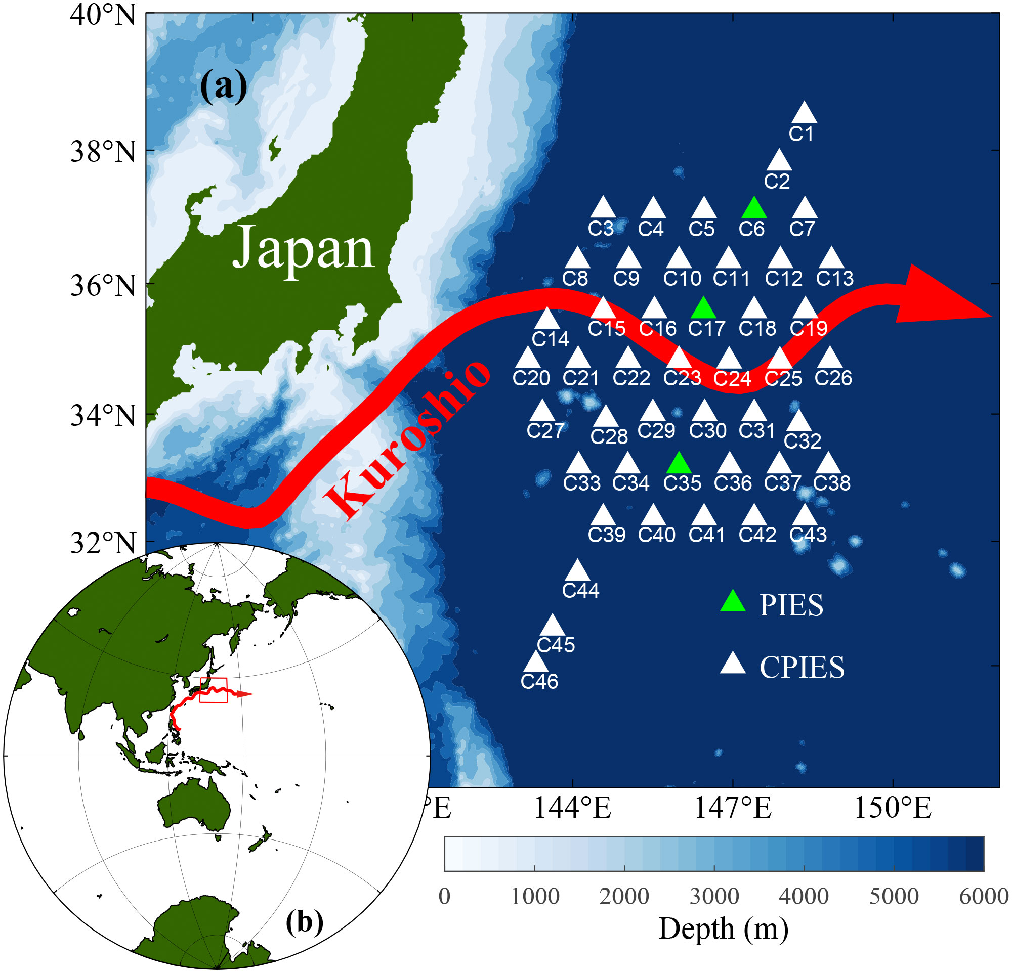
Figure 1 Schematic diagram of the Kuroshio Extension System Study (KESS) observation array. White and green triangles indicate pressure-equipped inverted echo sounders (PIESs) and current- and pressure-equipped inverted echo sounders (CPIESs), respectively [region shown in (A) is indicated by the red box in (B)].

The PIES is a bottom-anchored instrument which observes round-trip acoustic travel time from the sea bottom to surface, and bottom pressure. The CPIES is a PIES further equipped with an Aanderaa current meter, which can observe current velocity 50 m above the bottom (Zheng et al., 2021; Zhao et al., 2022). The CPIES transmits four acoustic signals every 10 min with a resolution of 0.03 ms; the bottom pressure sampling interval is 10 min, with an accuracy of 0.01% of the maximum range of the transducer, i.e., 0.6 dbar (1 dbar = 1 × 10⁴ Pa) and the current meter sampling interval is 20 min, with an absolute accuracy of ± 0.15 cm/s (Donohue et al., 2010). The KESS project publishes 72 h low-pass filtered and 12 h interval round-trip acoustic travel times from the sea surface to 1,400 dbar (τ₁₄₀₀ ), bottom pressure anomaly and current velocities (http://www.po.gso.uri.edu/dynamics/kess/CPIES_data.html; Kennelly et al., 2008). Of these, the error of τ₁₄₀₀ is 1.02 ms (Kennelly et al., 2008) and that of the current velocity is 1.5 cm/s (Donohue et al., 2010). The temperature, salinity, and current in the study region were mapped based on the above data.

2.1.2 Historical hydrographic profiles

A total of 15,881 historical hydrographic profiles with depths exceeding 1,400 dbar were collected in the study region (28–40°N, 141–151°E) for the gravest empirical mode (GEM) fields. Of these, 14,934 Argo profiles were obtained from the China Argo Real-Time Data Center (http://www.argo.org.cn), with most of the Argo profiles observed at depths less than 2,000 dbar; 607 CTD profiles were obtained from the World Ocean Database and 340 CTD profiles from the KESS cruise. A total of 319 CTD profiles reached over 4000 dbar.

2.1.3 Other data

Absolute dynamic topography (η) with temporal and spatial resolutions of 1 day and 0.25° × 0.25°, respectively, from the Copernicus Marine Environment Monitoring Service (https://resources.marine.copernicus.eu/products) was used to calculate surface geostrophic currents. The surface geostrophic currents (u_g and v_g) can be obtained from η as follows:

$\begin{array}{ll}{u}_g=-\frac{g}{f}\frac{\partial \eta }{\partial y}& (1)\end{array}$

$\begin{array}{ll}{v}_g=\frac{g}{f}\frac{\partial \eta }{\partial x}& (2)\end{array}$

where gravitational acceleration g = 9.8 m/s² and Coriolis parameter f=7.292×10⁻⁵ s⁻¹ .

Wind stress data from the Copernicus Marine Environment Monitoring Service with temporal and spatial resolutions of 6 h and 0.25° × 0.25°, respectively, were also used for diagnosing mesoscale eddy energy budgets.

2.2 Methods

2.2.1 Construction of temperature and salinity fields

The GEM method, which is an empirical lookup table from historical hydrographic profiles, was applied to obtain temperature, salinity, and specific volume anomaly fields from CPIES observations (Watts et al., 2001). Following Donohue et al. (2010), we constructed a GEM lookup table based on  τ₁₄₀₀ (Figure 2). The maximum error in temperature and salinity occurred at 0–200 dbar, with τ₁₄₀₀ ranging from 1.86–1.88 s, which was generally consistent with Donohue et al. (2010). Smaller errors appeared in the deep ocean; temperature (salinity) errors were 0.55, 0.16, and 0.03°C (0.10, 0.03, and 0.01) at 500, 1,000, and 2,000 dbar, respectively.

FIGURE 2

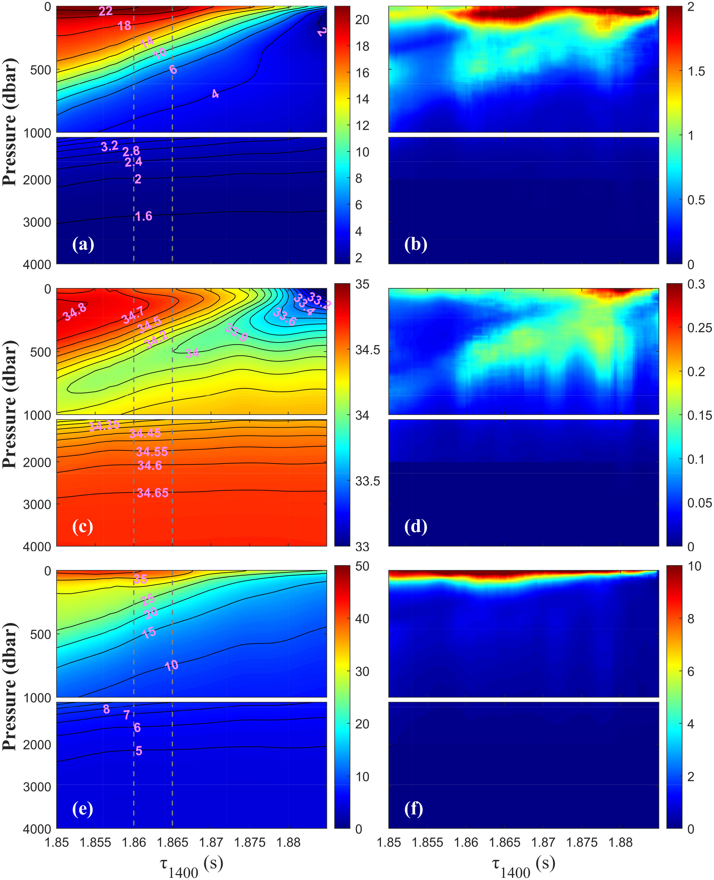
Figure 2 Gravest empirical mode (GEM) fields for (A) temperature, (C) salinity, and (E) specific volume anomalies in the Kuroshio Extension System Study (KESS) area and their root mean square difference (RMSD) (B, D, and F, respectively). Gray dashed lines frame the Kuroshio water.

Optimum interpolation (Bretherton et al., 1976; Zheng et al., 2021; Zheng et al., 2022b) was used to obtain the distribution of τ₁₄₀₀ in the observation area, which was further used to obtain the 3D temperature and salinity fields using the GEM method. Following Donohue et al. (2010), the mean and residual fields of τ were interpolated separately; the correlation length of the mean field (residual field) was determined to be 200 km (130 km), and the noise-to-signal variance ratios were 0.96 (0.34) for the interpolation.

2.2.2 Construction of current velocity fields

Considering that the number of deep historical hydrological profiles is limited and the baroclinic variation in the deep ocean is negligible, 4,000 dbar was chosen as the reference level. The absolute current velocity fields consisted of the barotropic current velocity field at 4,000 dbar and the baroclinic geostrophic current velocity relative to 4,000 dbar. The barotropic current velocity field is obtained by optimal interpolation of the seabed pressure observed by CPIES and the current field at 50 m from the bottom. The baroclinic current velocity field is obtained using the GEM method. The baroclinic geostrophic current velocity at a certain depth (h dbar) relative to the reference level is obtained by the following equation:

$\begin{array}{ll}\{\begin{array}{c}{u}_h=-\frac{1}{f}\left(\underset{-4000}{\overset{-h}{\int }}\frac{\partial \delta }{\partial y}dp\right)\\ v_h=\frac{1}{f}\left(\underset{-4000}{\overset{-h}{\int }}\frac{\partial \delta }{\partial x}dp\right) \end{array}& (3)\end{array}$

Where u_h and v_h are the eastward and northward components of the baroclinic geostrophic current velocity relative to the 4,000 dbar at h dbar, δ is specific volume anomaly.

2.2.3 Eddy detection method

High-resolution three-dimensional (3D) temperature, salinity, and current fields from numerical simulations have been used to develop methods for detecting and studying the structure of mesoscale eddies (Nencioli et al., 2010; Dong et al., 2012; Lin et al., 2015). Following the method used in the modeling current fields, the center and boundary of the mesoscale eddy were detected based on the CPIES-observed horizontal current fields. The eddy center was detected based on four conditions: 1) opposite directions of meridional flow to the east and west of the eddy center, and flow velocity increases farther away from the center; 2) opposite directions of zonal flow to the north and south of the eddy center, and the flow velocity increases farther away from the center; 3) velocity minimum point in the selected area is approximated as the eddy center; and 4) rotation direction of the velocity vector is the same as that in the vicinity of the approximate eddy center. An eddy is considered to exist if an eddy center meets the above conditions. The eddy boundary is defined as the outermost closed stream function. The relationship between the stream function ψ and the horizontal velocity is as follows:

$\begin{array}{ll}u=-\frac{\partial \psi }{\partial x}, v=\frac{\partial \psi }{\partial y}& (4)\end{array}$

Where u and v are the meridional and zonal current velocities, respectively.

To obtain a 3D structure of an eddy, detection was run separately for each vertical layer. If eddies in two adjacent layers had the same polarity and the horizontal distance of the eddy centers was less than 100 km, it was considered as the same eddy. If the eddy was not detected for 200 m, the detection was stopped.

The radius R of the eddy is defined as:

$\begin{array}{ll}R=\sqrt{\frac{S}{\pi }}& (5)\end{array}$

where S is the area enclosed by the eddy boundary. The eddy depth is defined as the maximum depth at which the eddy can be detected.

3 Results

3.1 3D structure

The eddy detection from CPIES observations and from satellite observations show similar temporal and spatial variation (Figure 3). Compared with satellite observations, the root mean square difference (RMSD) of both u and v were 0.2–0.3 m/s, the eddy center difference was less than 30 km, and the eddy boundaries were similar, indicating the accuracy of CPIES observed mesoscale eddy structures.

FIGURE 3

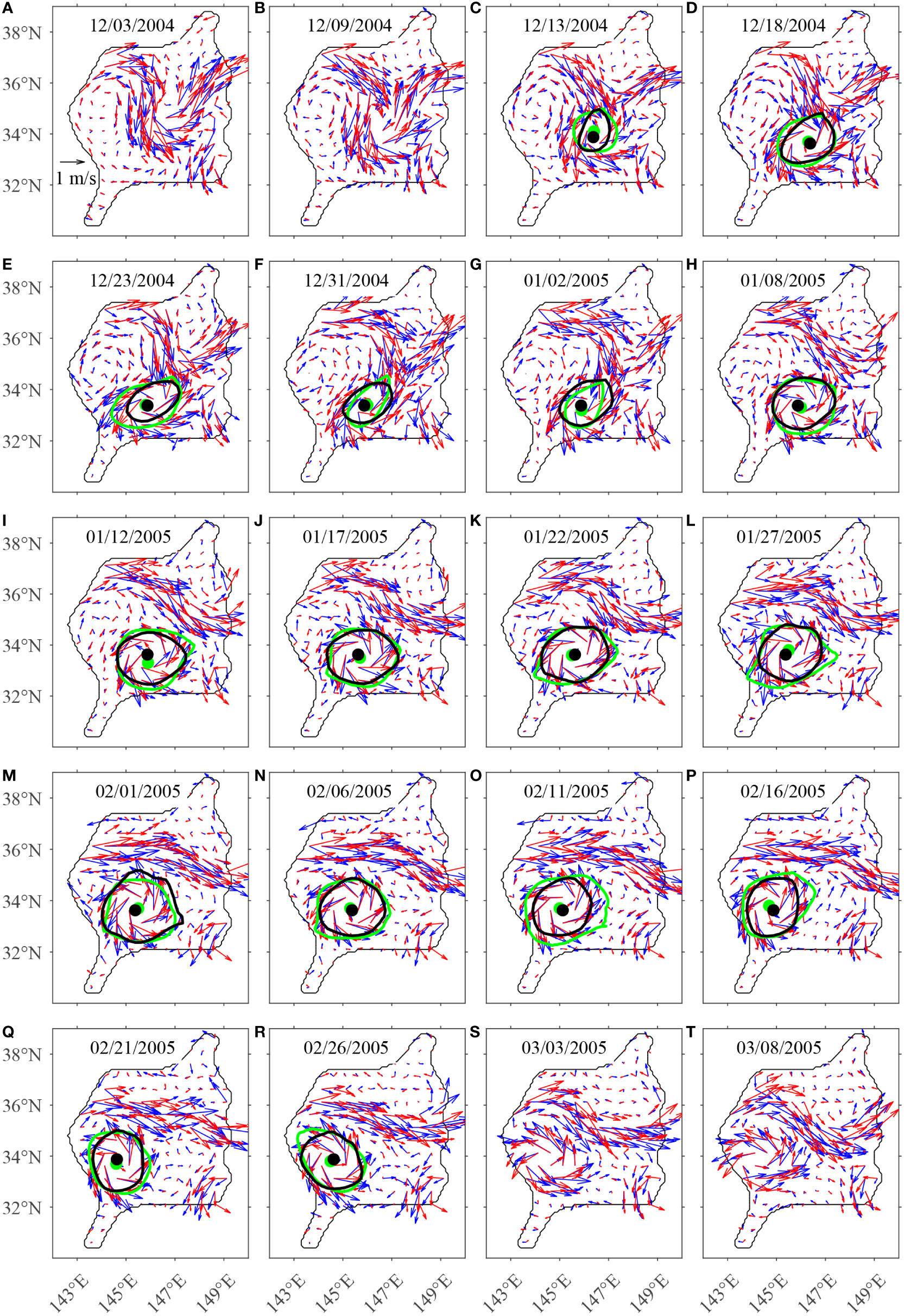
Figure 3 Comparison of the surface currents from the satellite altimeter (red) and Kuroshio Extension System Study (KESS) observations (blue). The thin black line shows the observation area, the thick green and black lines mark the current- and pressure-equipped inverted echo sounder (CPIES)-detected and satellite-detected eddy boundaries, respectively.

On December 9, 2004, the Kuroshio curved southward and formed a nearly circular cyclonic eddy (Figure 3B). Subsequently, the eddy grew rapidly near 146°E, 34°N and was completely shed off from the Kuroshio main axis on January 8, 2005 (Figure 3H). The eddy was nearly circular and moved westward at an average speed of 7.4 km/d in the next 2 months. The CPIES array captured the complete structure of the eddy during December 2004–February 2005. In March, part of the eddy had left the CPIES array (Figures 3S, T) and is therefore not discussed in the study. The variability of the eddy over a total of 83 days from generation to the time it partially left the observation area was studied.

On February 1, 2005, the eddy, which had completely shed from the Kuroshio (Figure 3M), was detected as an example to show the 3D structure of the eddy during its stable period. The axis of the eddy was tilted possibly owing to the topography β effect (Zhang et al., 2016; Shu et al., 2018), and the deviation of the eddy center position increased with depth relative to the surface layer, reaching 28.9 km and 76.2 km at 1,000 m and 2,000 m, respectively (Figure 4A). The eddy velocity decreased from top to bottom, with mean (maximum) current velocities at 0, 500, 1,000, 1,500, and 2,000 dbar of 1.18 (1.94), 0.64 (1.25), 0.24 (0.51), 0.14 (0.30), and 0.10 (0.26) m/s, respectively.

FIGURE 4

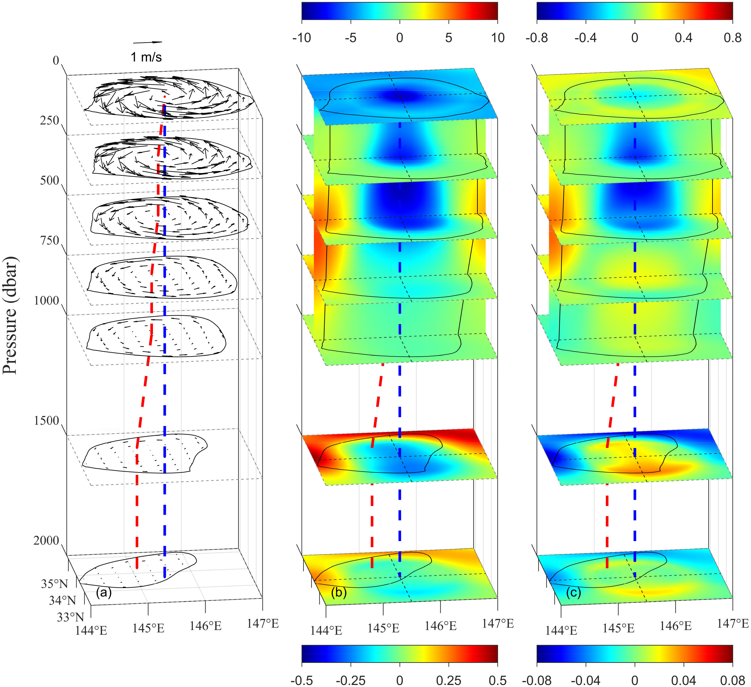
Figure 4 Three dimensional view of the (A) velocity (m/s), (B) temperature anomaly (°C), and (C) salinity anomaly (psu) structure of the eddy on February 1, 2005. The red dashed line connects the eddy centers, the blue dashed line is the projection of the surface eddy center on each layer, and the black line indicates the eddy boundary at each layer.

As shown in Figures 4B, C, only a slight variation in temperature and salinity was observed from 1,500 to 2,000 dbar; therefore, the temperature and salinity structure in the deep ocean is not further discussed. A marked conical cold temperature anomaly core existed in the eddy above 1,000 dbar (Figure 4B), with a maximum anomaly of -9.1°C at 360 dbar. The salinity anomaly had a vertical dipole structure with a boundary at 600 dbar. There was a conical negative anomaly core in the upper layer, with a maximum anomaly (-0.68) at 340 dbar. A positive anomaly lay in the lower layer, with a maximum anomaly (0.20) at 780 dbar (Figure 4C). The temperature and salinity anomalies in the eddy were resulted from the water property differences between two sides of the Kuroshio. The eddy packaged cold Oyashio water to the south, which caused the cold temperature anomaly core. The Oyashio water showed lower and higher salinity in the upper layer and below ~ 600 dbar, respectively, which resulted in the vertical dual-core salinity anomaly.

The kinetic energy ($\frac{1}{2}\left(u^2+v^2\right)$) decreased from the surface to bottom and was greater on the boundary than at the center of the eddy (Figure 5A). The stream function (Ψ) coordinate was used to show the distribution of each parameter clearly. The Ψ is set to 0 at the eddy center (Figures 5E–H). The kinetic energy, vorticity ($\zeta =\frac{\partial v}{\partial x}-\frac{\partial u}{\partial y}$), temperature, and salinity in the stream function coordinate were less discrete than those in the traditional distance coordinates (not shown). Under the stream function coordinates, the kinetic energy of the eddy first increased and then decreased from the inside to the outside at all depths. Taking the surface layer as an example, the mean kinetic energy reached a maximum value (1.27 m²/s²) at a stream function Ψ = -1.45 × 10⁵ m²/s and decreased to 0.37 m²/s² at the eddy boundary (Ψ = -2.50 × 10⁵ m²/s), and the distribution of kinetic energy under stream function coordinates showed an arc shape (Figure 5E). As the kinetic energy was higher in the northwest and lower in the southeast on the eddy boundary, the same stream function corresponded to different kinetic energies. At the same stream function, the stronger the anisotropy was, the more discrete the kinetic energy distribution was. In the center of the eddy, the anisotropy was not notable, and the kinetic energy was similar under the same stream function coordinates; however, the currents at the eddy boundary was influenced by the Kuroshio, and the velocity in the same stream contour line varied in different directions and kinetic energy was more discrete under the stream function coordinates. This phenomenon was highly notable below the subsurface. The vorticity showed largest value near the eddy center, and decreased when leaving the center (Figures 5B, F). When close to the eddy boundary, the vorticity nearly decreased to 0. Although similar spatial variance was identified in different layers, the lower layer showed smaller vorticity than the upper layer.

FIGURE 5

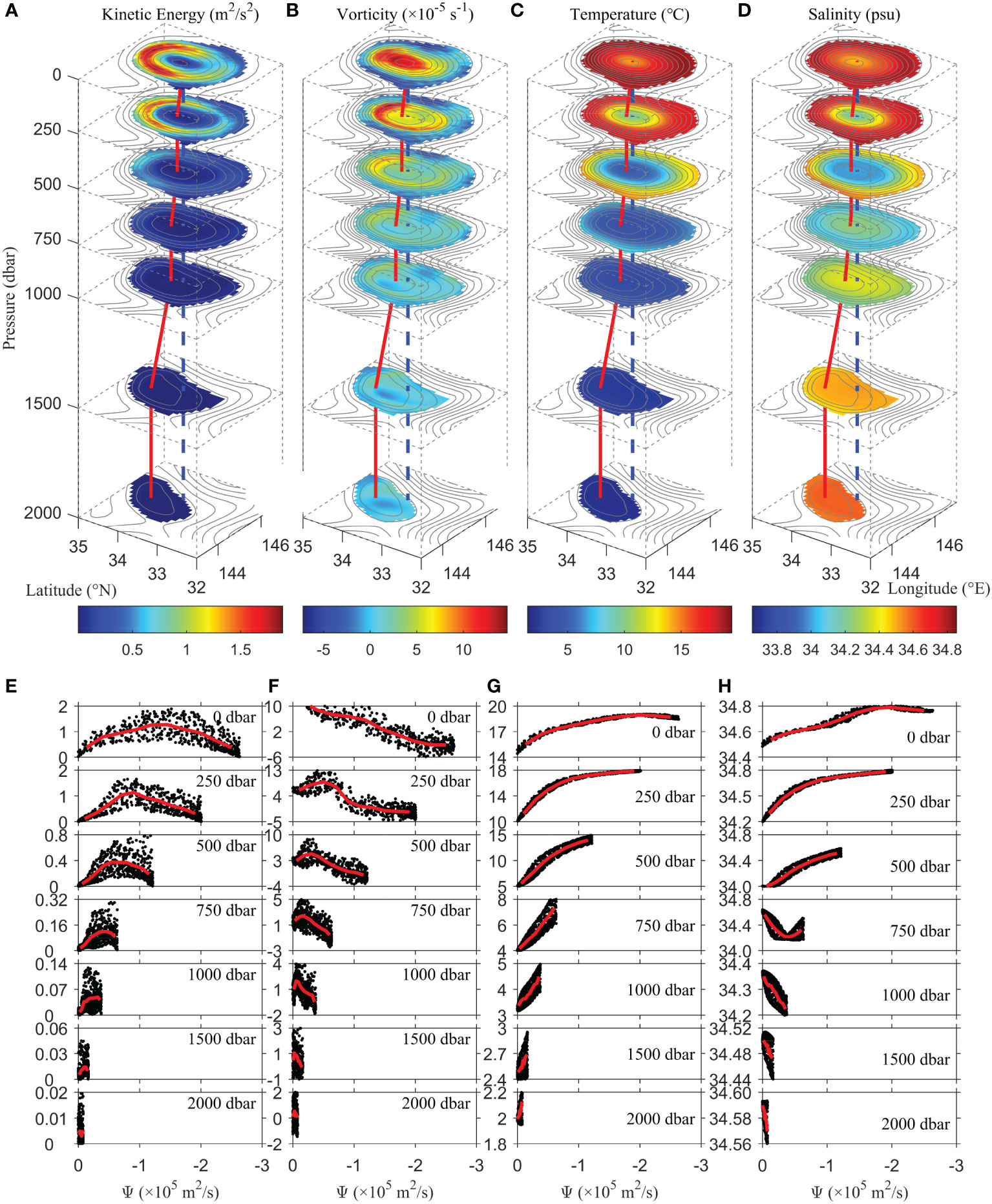
Figure 5 Three-dimensional structure of (A) eddy kinetic energy ($\frac{1}{2}\left(u^2+v^2\right)$), (B) vorticity ($\zeta =\frac{\partial v}{\partial x}-\frac{\partial u}{\partial y}$), (C) temperature, and (D) salinity on February 1, 2005 at 0, 250, 500, 750, 1,000, 1,500, and 2,000 dbar. Blue dashed line marks the vertical projection of the surface eddy center, and red solid line connects the eddy centers in the layers. Gray lines indicate the contours of the stream function of each layer relative to the eddy center. (E–H) Black dots correspond to the stream function values at depth with respect to kinetic energy, vorticity, temperature, and salinity. Red solid line indicates the mean value at the stream function per 1 × 10^-6 m²/s.

The temperature for each layer increased outward from the center (Figures 5C, G), with the temperature difference between the inside and outside of the eddy reaching a maximum (8°C) at 500 dbar. The salinity increased outward above approximately 600 dbar, whereas decreased outward at depths deeper than 600 dbar (Figure 5D, H), which is consistent with the dual-core structure of the salinity anomaly in Figure 4C. The difference in salinity between the inside and outside of the eddy could be up to 0.6 psu.

3.2 Temporal variation

Before January 8, 2005, when the eddy had not been completely shed from the Kuroshio, the eddy showed radii varying from 20 to 60 km (Figure 6A). The depth of the eddy was less than 2,000 dbar before December 29, 2004; however, it increased considerably thereafter. After shedding from the Kuroshio, the radius reached 60–80 km, and the depth of the eddy decreased. In early January 2005, the eddy depth was approximately 3,000 dbar, whereas in February it decreased to 2,000 dbar. Although the surface eddy was captured by the CPIES array, the eddy in the deep ocean might have left the study region by the end of February owing to the westward tilt of the vertical axis, which caused the decrease in the detected depth of the eddy. The total volume of the eddy remained stable after it shed from the Kuroshio on January 8, 2005. Temporal changes in eddy volume were highly consistent with the changes in eddy mass and heat (Figures 6B–C). The heat anomaly first changed with volume before January 8, 2005, and then decreased slowly overall (Figure 6C). The total salt anomaly in the eddy increased with volume in mid-December, stabilized from late December to mid-January, and continued to decrease slowly from late January (Figure 6D). The variances in total kinetic energy ($\frac{1}{2}{\int }^{}\rho \left(u^2+v^2\right)dV$) and vertical averaged vorticity flux were also similar with that of volume (Figures 6E, F); they first increased then decreased in December 2004, and were stable after shedding from the Kuroshio.

FIGURE 6

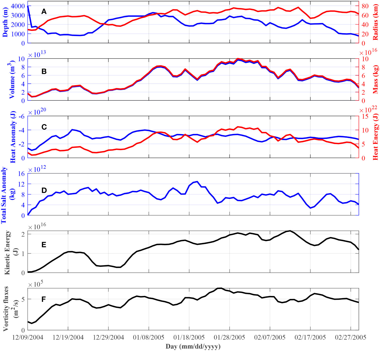
Figure 6 Time series of (A) depth and mean radius of the eddy, (B) total mass and volume, (C) total heat for the eddy and its anomalies, (D) total salt anomalies, (E) total kinetic energy ($\frac{1}{2}{\int }^{}\rho \left(u^2+v^2\right)dV$), and (F) vertical averaged vorticity fluxes from December 9, 2004 to March 1, 2005. Total salt is calculated as the salinity multiply by the total mass of the eddy. Anomalies are calculated as the daily value minus the 1-year average at that location.

4 Discussion

The full water depth currents obtained from CPIES observations provides an opportunity to analyze the eddy energy budget during generation and movement. According to Oey (2008), the eddy energy evolution can be calculated by the following equation:

$\begin{array}{ll}\begin{array}{l}\frac{d}{dt}\int \left[\frac{1}{2}\overline{v{\prime }^2}+\frac{g^2\overline{\rho {\prime }^2}}{2N^2{\rho }_0^2}\right]dz=\frac{1}{\rho }\overline{{\tau }_w·v_{top}^{\prime }}-\int \frac{g^2}{{\rho }_0^2{N}^2}\overline{v^{\prime }{\rho }^{\prime }}·\nabla \overline{\rho }dz\\ -\int (\frac{\partial \overline{u}}{\partial x}·\overline{u{\prime }^2}+\frac{\partial \overline{v}}{\partial y}·\overline{v{\prime }^2}+\overline{u\prime v\prime }·\frac{\partial \overline{v}}{\partial x}+\overline{u^{\prime }{v}^{\prime }}·\frac{\partial \overline{u}}{\partial y})dz-\int \nabla ·\left(\frac{\overline{v^{\prime }{\rho }^{\prime }}}{{\rho }_0}\right)dz-\int \left(\overline{w\prime u\prime }·\frac{\partial \overline{u}}{\partial z}+\overline{w\prime v\prime }·\frac{\partial \overline{v}}{\partial z}\right)dz\end{array}& (6)\end{array}$

The left-hand of the equation shows the time variation of the total eddy energy (EE), and the first and second terms in the middle bracket are the eddy kinetic energy (EKE) and eddy potential energy (EPE), respectively. The overbar indicates the 30-day smoothing average. On the right side are the energy terms. The first term of the right-hand of the equation is wind stress work (WW), where τ_w is wind stress, v_top is the surface current, and ' represents the anomaly in which the time average was removed. The second and third terms of the right-hand of the equation are baroclinic conversion (BC) and barotropic conversion (BT), respectively. When these terms are positive, the mean flow energy is converted to eddy energy. The fourth and fifth terms are the pressure perturbation term and Kelvin–Helmholtz instability, respectively, which are not discussed in this paper because their values were considerably smaller than those of the other parameters (Zhang et al., 2013b). The square of the buoyancy frequency $N^2=-\frac{g}{\rho }\frac{d\rho }{dz}$ was obtained from the profiles obtained from the GEM. The average density of seawater was considered as ρ₀ = 1,030 kg/m³.

The temporal variations in the distribution of eddy energy (EKE and EPE) and energy terms (ADV, BC, BT, and WW) in the observed region are shown in Figure 7. ADV= ∫ v·∇ EE dz is the advective term of the total EE, representing the variation caused by the EE transported through advection. Considering that each energy term is small and negligible below 2,000 m, all terms except WW are integrated from 0 to 2,000 m.

FIGURE 7

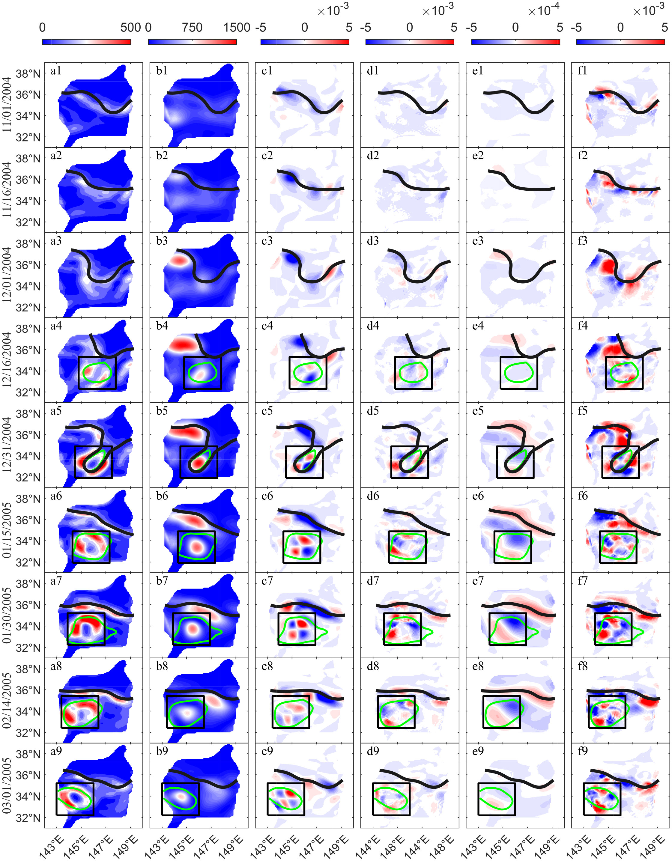
Figure 7 Daily maps of (A) eddy kinetic energy (EKE, m³/s²), (B) eddy potential energy (EPE, m³/s²), (C) baroclinic conversion (BC, m²/s²), (D) barotropic conversion (BT, m²/s²), (E) wind stress work (WW, m²/s²), and (F) advective term (ADV, m²/s²) patterns. The black line represents the Kuroshio axis, the green circle marks the eddy boundary, and the black box is a 3° × 3° concentric square with the eddy.

The EKE became strong on the south of the Kuroshio in November 2004 (Figures 7A1–3), which was the initial energy source of the eddy. The EPE at the region where the Kuroshio meanders, was increased at the same time (Figures 7B1–3). Both EKE and EPE increased after the formation of the eddy but decreased after February 2005 (Figures 7A1–9 and B1–9). High EKE values were mainly observed along the boundary of the eddy (Figures 7A6–9), whereas the high-EPE area was concentrated near the center of the eddy (Figures 7B6–9). During November and early December 2004, BC was negative in regions with high eddy energy (Figures 7C1–3), suggesting that the EPE was converted to mean available potential energy. The BT was smaller and negative (Figures 7D1–3), indicating that the EKE was converted to mean kinetic energy. High positive values of ADV occurred during this period (Figures 7F1–3), indicating that EE originates mainly from Kuroshio advection transport and is reduced through BC and BT. After the eddy completely separated from the Kuroshio, the BC inside the eddy had a dual-dipole structure (Figure 7C6), with a positive value at the northeast/southwest and a negative value at the northwest/southeast. All four poles were located at the boundary of the high-EPE region within the eddy (Figures 7B6, C6), indicating that the conversion of EPE to mean available potential energy occurs mainly at the boundary of the high-EPE region, and compared with adjacent quadrants, showed opposite energy conversion. The BT was mainly distributed at the boundary of the high EKE region (Figures 7 A6, D6), which indicates that the conversion of EKE to mean kinetic energy occurs at the boundary region with high EKE. The WW (Figures 7E1–9) was one order smaller than BC and BT (Figures 7); therefore, its effect was negligible. The above results suggest that the exchange between eddy and mean flow energy was mainly caused by barotropic and baroclinic instabilities, which is consistent with the results of previous studies on BC-driven eddies in the regions of the North Atlantic Current (White and Heywood, 1995).

To quantify the role of each energy term during evolution of the eddy, we integrated the terms EKE, EPE, BC, BT, ADV, and WW in the black box in Figure 7, which is showed in Figure 8. Figure 8A shows that the EPE increased markedly after January 15, 2005 and reached a maximum at the end of January, and the EKE increased gradually from December and reached a maximum almost simultaneously with the EPE. During the first 10 days of eddy formation, the ADV was high (Figure 8B), indicating that the EE was primarily sourced from advection. Therefore, the Kuroshio is speculated to be the source of EE. In general, BT was negative in the first 10 days, which means that EKE is converted to mean kinetic energy. BC also performed negative work at these period, indicating that EPE converted to mean available potential energy. From late December to early March, BT continued to positive values, converting mean kinetic energy to EKE. As shown in Figure 3F, the eddy was stretched in the north–south direction and compressed in the east–west direction in late December, causing a narrow elliptical boundary and a minimum radius (Figure 6A). The negative BC reached its minimum in this period, i.e., the eddy energy was lost to the mean available potential energy more rapidly during the eddy stretching process. The ADV reached a peak at similar time (Figure 8B), possibly caused by the violently deformation of the eddy (Figure 7F5). The eddy shape returned to nearly circular in early January, and the eddy was completely shed on January 8 (Figure 3H). During this process, BC increased to near 0, and EPE was no longer lost to mean available potential energy. After the eddy was shed off in mid-January, BC in the eddy generally did positive work, and the mean available potential energy was converted to EPE; however, the contribution was small compared to that of BT, i.e., BT played a major role after the eddy was stabilized. After February 20, because the eddy was close to the boundary of the CPIES array, calculations of energy terms were subject to errors; hence, they are not discussed in the study.

FIGURE 8

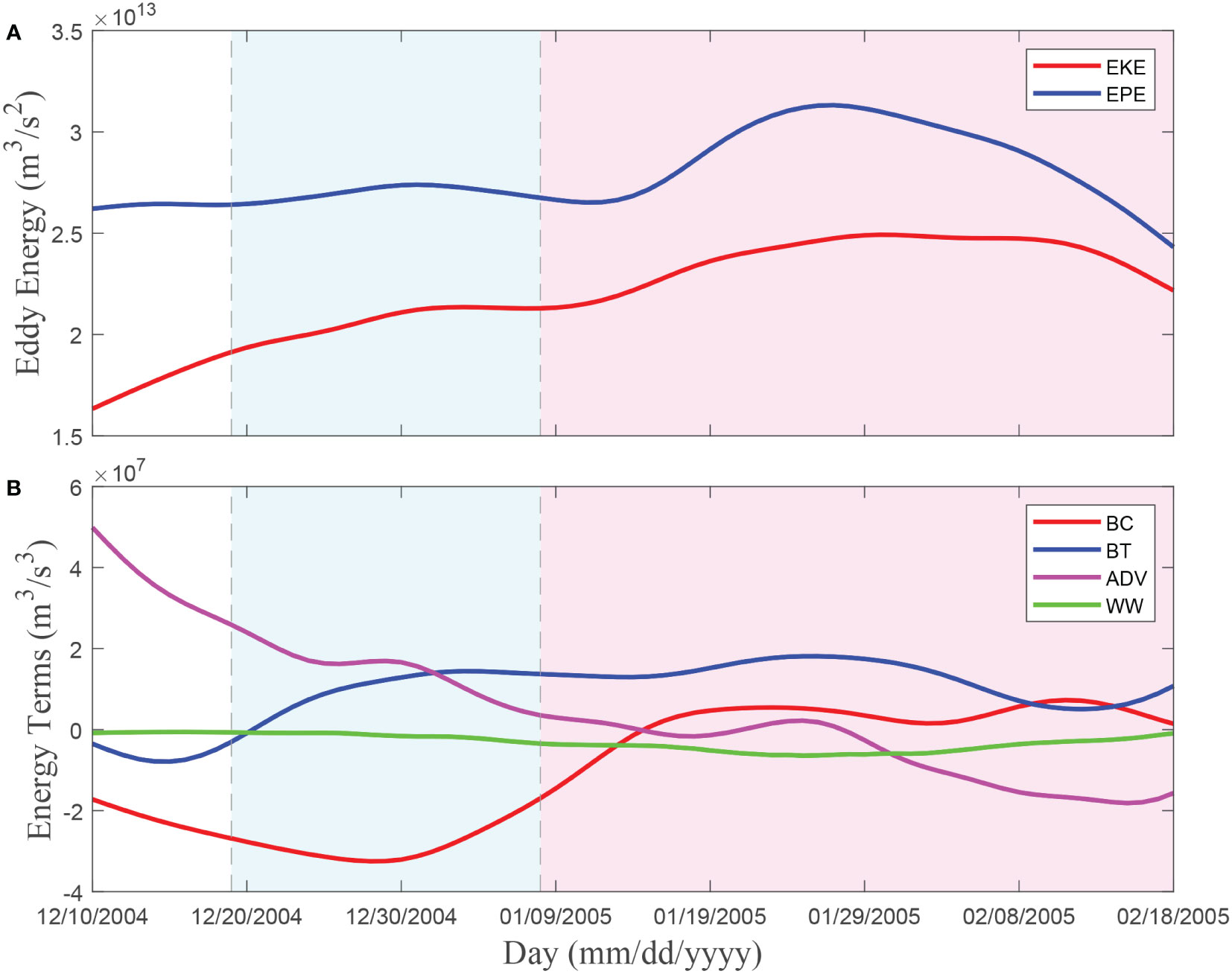
Figure 8 Time series of the plane integrals of the energy terms in the region where the eddy is located (black box in Figure 7). (A) shows eddy kinetic energy (EKE) and eddy potential energy (EPE), and (B) shows baroclinic conversion (BC), barotropic conversion (BT), advective term (ADV), and wind stress work (WW) values. White, cyan and pink background color indicate the periods of generation, separation, and stabilization, respectively.

The main source of EE in the ocean is considered to be BC (Wang and Ikeda, 1997; Stammer, 1998). Both BC and BT are important energy sources for anticyclonic eddies shedding from the Kuroshio near the Luzon Strait (Zhang et al., 2013b). Sub-mesoscale ageostrophic motion play important roles in the Kuroshio intrusion zone and was thought to enhance the strength of eddies (Qiu et al., 2022b). Unlike in the previously mentioned studies, in the present study, advective transport of kinetic energy originating from the Kuroshio was the main energy source of the eddy during generation and development, whereas BC and BT dissipated the eddy energy. After the eddy shed off from the Kuroshio, BC and BT converted mean flow energy to EE, which further enhanced EKE and EPE.

The KE is one of two high-energy eddy regions in the North Pacific; however, previous studies of eddies here have mostly been based on satellite altimetry (Ichikawa and Imawaki, 1994; Itoh and Yasuda, 2010; Chu et al., 2017; Ji et al., 2018), satellite sea surface temperatures (Dong et al., 2011a), and drifter trajectories from the Global Drifter Program (Dong et al., 2011b). The investigation of the deep structure of eddies is lacking in these studies. The 3D structure of the mesoscale eddies presented in this paper exhibits a monopole structure for temperature and a dipole structure for salinity in the vertical direction, which is similar to the vertical structure of the mesoscale eddies south of the KE, based on previous studies like the Argo as well as underway observations (Sun et al., 2017; Dong et al., 2017; Zhang et al., 2019). This suggests that the mesoscale eddies in this region may have a similar 3D-structure and water characteristics. Compared with the 3D-structure composited from Argo profiles (Sun et al., 2017; Dong et al., 2017), the CPIES-observed structure showed detailed horizontal variance and vertical structure of temperature single-core and salinity double-core structures. The detailed 3D structure of the eddy temperature, salinity, and currents is similar to the 3D structure of the eddy obtained by Zhang et al. (2019) based on underway observations in the KE; however, in the present study, the detailed process of the evolution of eddy generation and westward propagation was additionally obtained. Compared to the eddies observed by Zhang et al. (2019), the eddies in the present study are located further west. Both have almost the same depths of temperature and maximum and minimum salinity; however, the eddies in the present study were found to have greater temperature and salinity anomalies. This may be owing to the greater temperature and salinity differences between the two sides of the Kuroshio where the eddies were produced. The eddy studied here had a maximum temperature anomaly of -9.1°C, which was much larger than that in other areas such as in the South China Sea (-6.1°C; Zhang et al., 2013b), east of the Ryukyu Island chain (-3.0°C; Zhu et al., 2008), and the KE region (-7.3°C; Zhang et al., 2019). To the best of our knowledge, the temperature anomaly of the eddy presented in the present study is the strongest in the North Pacific Ocean and its adjacent seas; thus, the eddy is supercharged.

5 Conclusion

The KE is a region with high mesoscale eddy occurrence. In the present study, based on the CPIES observations acquired by KESS, we conducted the first long-term, continuous, full-depth simultaneous detection of the 3D structure of a supercharged mesoscale eddy generated from Kuroshio in December 2004. In early December, the Kuroshio meandered southward, and the Kuroshio water wrapped around cold water from the north, which shed to form a cold eddy. In early January of the following year, the structure stabilized after completely detaching from the Kuroshio. After stabilization, the eddy exhibited a radius of 60–80 km, depth up to 3,000 dbar, and propagated westward with a speed of 7.4 km/d.

The eddy had a negative temperature anomaly above 1,000 dbar with an anomaly maximum of -9.1°C at a depth of 360 dbar. The salinity anomaly had a vertical dual-core structure, i.e., a negative anomaly above 600 dbar and a positive anomaly below this depth. The negative and positive anomalies at 780 dbar and 340 dbar were -0.68 psu and 0.20 psu, respectively. Under the stream function coordinate, kinetic energy of the eddy first increased and then decreased from the center toward the boundary, whereas the vorticity decreased overall.

The present study first shows the temporal variation in the main parameters of an eddy throughout its generation, development, and stabilization period based on in situ observations. The radii and depth of the eddy gradually increased during the generation and development period before complete shedding from the Kuroshio. During its stabilization period after shedding, the temporal variations in eddy volume, heat, kinetic energy, and vorticity flux were highly consistent. The heat and salt anomalies of the eddy gradually decreased with time, and the temperature and salinity in the eddy tended to match those of the surrounding water, indicating the existence of material and energy exchanges between the eddy and the external environment.

Eddy energy changes were mainly influenced by ADV, BT, and BC, with minimal influence from WW. During eddy formation, the EKE transported by the Kuroshio was the initial source of energy for eddy formation, whereas BC and BT played a dissipative role in converting EPE to mean available potential energy. When the eddy stretched in late December, BC reached its minimum value and EPE was converted to mean available potential energy at an accelerated rate, and ADV intensified and reached its peak value. After the eddy was completely shed and stabilized, BC appeared as a dual-dipole structure at the boundary of the high-EPE region in the eddy, and BT varied positively and negatively in different directions at the outer side of the high EKE region. Overall, BC and BT did positive work to convert mean kinetic energy to EKE, resulting in a considerable increase in EPE and EKE.

Based on CPIES observations, the present study obtained the 3D structure of parameters including temperature, salinity, and currents over a sustained period, which were used to calculate the distribution of vorticity, kinetic energy, and other parameters as well as their temporal variation, thereby elucidating the energy conversion mechanisms in eddy generation, development, and stabilization. These findings deepen our knowledge of the 3D structure of eddies in the KE region and are important for studying the influence of eddies on the mixed layer, thermocline, and STMW as well as the ecological effects of eddies in the region.

Data availability statement

Publicly available datasets were analyzed in this study. This data can be found here: http://www.po.gso.uri.edu/dynamics/kess/CPIES_data.html.

Author contributions

XZ and X-HZ contributed to conception and design of the study. XZ performed the data analysis. XZ, X-HZ, HZ wrote the first draft of the article. RZ, CX, JC, MW gave comments for revising the article. All authors contributed to the article and approved the submitted version.

Acknowledgments

The authors are grateful to the KESS project for sharing their data (http://www.po.gso.uri.edu/dynamics/kess/CPIES_data.html).

Funding

This study was sponsored by the National Natural Science Foundation of China (Grants 41920104006 and 41976001), the Scientific Research Fund of Second Institute of Oceanography, MNR (Grants JZ2001 and QNYC2102), the Project of State Key Laboratory of Satellite Ocean Environment Dynamics, Second Institute of Oceanography (SOEDZZ2106 and SOEDZZ2207), the Oceanic Interdisciplinary Program of Shanghai Jiao Tong University (Project SL2021MS021), and the Innovation Group Project of Southern Marine Science and Engineering Guangdong Laboratory (Zhuhai) (311020004).

Conflict of interest

The authors declare that the research was conducted in the absence of any commercial or financial relationships that could be construed as a potential conflict of interest.

Publisher’s note

All claims expressed in this article are solely those of the authors and do not necessarily represent those of their affiliated organizations, or those of the publisher, the editors and the reviewers. Any product that may be evaluated in this article, or claim that may be made by its manufacturer, is not guaranteed or endorsed by the publisher.

References

Benitez-Nelson C. R., Bidigare R. R., Dickey T. D., Landry M. R., Leonard C. L., Brown S. L., et al. (2007). Mesoscale eddies drive increased silica export in the subtropical pacific ocean. Science. 316, 1017–1021. doi: 10.1126/science.1136221

PubMed Abstract | CrossRef Full Text | Google Scholar

Bishop S. P., Watts D. R. (2014). Rapid eddy-induced modification of subtropical mode water during the kuroshio extension system study. J. Phys. Oceanogr. 44, 1941–11953. doi: 10.1175/JPO-D-13-0191.1

CrossRef Full Text | Google Scholar

Bretherton F. P., Davis R. E., Fandry C. B. (1976). A technique for objective analysis and design of oceanographic experiments applied to MODE-73. Deep-Sea Res. Oceanogr. Abstr. 23 (7), 559–582. doi: 10.1016/0011-7471(76)90001-2

CrossRef Full Text | Google Scholar

Chaigneau A., Texier M. L., Eldin G., Grados C., Pizarro O. (2011). Vertical structure of mesoscale eddies in the eastern south pacific ocean: A composite analysis from altimetry and argo profiling floats. J. Geophys. Res. Oceans. 116, C11025. doi: 10.1029/2011jc007134

CrossRef Full Text | Google Scholar

Chelton D. B., Schlax M. G., Samelson R. M. (2011). Global observations of nonlinear mesoscale eddies. Prog. Oceanogr. 91 (2), 167–216. doi: 10.1016/j.pocean.2011.01.002

CrossRef Full Text | Google Scholar

Chelton D. B., Schlax M. G., Samelson R. M., Szoeke R. A. (2007). Global observations of large oceanic eddies. Geophys. Res. Lett. 34 (15), 87–101. doi: 10.1029/2007GL030812

CrossRef Full Text | Google Scholar

Chu X., Dong C., Qi Y. (2017). The influence of ENSO on an oceanic eddy pair in the south China Sea. J. Geophys. Res. Oceans. 122, 1643–1652. doi: 10.1002/2016JC01264

CrossRef Full Text | Google Scholar

Dong D., Brandt P., Chang P., Schutte F., Yang X., Yan J., et al. (2017). Mesoscale eddies in the northwestern pacific ocean: Three-dimensional eddy structures and heat/salt transports. J. Geophys. Res. Oceans. 122 (12), 9795–9813. doi: 10.1002/2017JC013303

CrossRef Full Text | Google Scholar

Dong C., Lin X., Liu Y., Nencioli F., Chao Y., Guan Y., et al. (2012). Three-dimensional oceanic eddy analysis in the southern California bight from a numerical product. J. Geophys. Res. Oceans. 117, C00H14. doi: 10.1029/2011JC007354

CrossRef Full Text | Google Scholar

Dong C. M., Liu Y., Lumpkin R., Lankhorst M., Chen D. K., McWilliams J. C., et al. (2011b). A scheme to identify loops from trajectories of oceanic surface drifters: An application in the kuroshio extension region. J. Atmos. Ocean Technol. 28 (9), 1167–1176. doi: 10.1175/JTECH-D-10-05028.1

CrossRef Full Text | Google Scholar

Dong C., McWilliams J. C., Liu Y., Chen D. (2014). Global heat and salt transports by eddy movement. Nat. Commun. 5 (1), 3328–3345. doi: 10.1038/ncomms4294

PubMed Abstract | CrossRef Full Text | Google Scholar

Dong C. M., Nencioli F., Liu Y., McWilliams J. C. (2011a). An automated approach to detect oceanic eddies from satellite remotely sensed sea surface temperature data. IEEE Geosci. Remote. Sens. Lett. 8 (6), 1055–1059. doi: 10.1109/LGRS.2011.2155029

CrossRef Full Text | Google Scholar

Donohue K. A., Watts D. R., Tracey K. L., Greene A. D., Kennelly M. (2010). Mapping circulation in the kuroshio extension with an array of current and pressure recording inverted echo sounders. J. Atmos. Ocean Technol. 27 (3), 507–527. doi: 10.1175/2009JTECHO686.1

CrossRef Full Text | Google Scholar

Gaube P., Barceló C., Mcgillicuddy D. J., Domingo A., Swimmer Y. (2017). The use of mesoscale eddies by juvenile loggerhead sea turtles (Caretta caretta) in the southwestern Atlantic. PloS One 12 (3), e0172839. doi: 10.1371/journal.pone.0172839

PubMed Abstract | CrossRef Full Text | Google Scholar

Gaube P., Chelton D. B., Samelson R. M., Schlax M. G., O'Neill L. W. (2015). Satellite observations of mesoscale eddy-induced ekman pumping. J. Phys. Oceanogr. 45 (1), 104–132. doi: 10.1175/JPO-D-14-0032.1

CrossRef Full Text | Google Scholar

Hu J., Gan J., Sun Z., Zhu J., Dai M. (2011). Observed three-dimensional structure of a cold eddy in the southwestern south China Sea. J. Geophys. Res. Oceans. 116, C05016. doi: 10.1029/2010JC006810

CrossRef Full Text | Google Scholar

Ichikawa K., Imawaki S. (1994). Life history of a cyclonic ring detached from the kuroshio extension as seen by the geosat altimeter. J. Geophys. Res. 99, 15953–115966. doi: 10.1029/94JC01139

CrossRef Full Text | Google Scholar

Itoh S., Yasuda I. (2010). Characteristics of mesoscale eddies in the kuroshio-oyashio extension region detected from the distribution of the sea surface height anomaly. J. Phys. Oceanogr. 40 (5), 1018–1034. doi: 10.1175/2009JPO4265.1

CrossRef Full Text | Google Scholar

Ji J., Dong C., Zhang B., Liu Y., Zou B., King G. P., et al. (2018). Oceanic eddy characteristics and generation mechanisms in the kuroshio extension region. J. Geophys. Res. Oceans. 123 (11), 8548–8567. doi: 10.1029/2018JC014196

CrossRef Full Text | Google Scholar

Kennelly M., Donohue K., Greene A., Tracey K. L., Watts D. R. (2008). “Report No.: 2008-02. Inverted echo sounder data report, Kuroshio Extension System Study (KESS). University of Rhode Island GSO Tech.

Google Scholar

Kurczyn J. A., Beier E., Lavín M. F., Chaigneau A., Godínez V. M. (2013). Anatomy and evolution of a cyclonic mesoscale eddy observed in the northeastern pacific tropical-subtropical transition zone. J. Geophys. Res. Oceans. 118, 5931–5950. doi: 10.1002/2013jc009339

CrossRef Full Text | Google Scholar

Lin X., Dong C., Chen D., Yu L., Guan Y. (2015). Three-dimensional properties of mesoscale eddies in the south China Sea based on eddy-resolving model output. Deep-Sea Res. Part I. 99, 46–64. doi: 10.1016/j.dsr.2015.01.007

CrossRef Full Text | Google Scholar

Li J., Wang G., Zhai X. (2017). Observed cold filaments associated with mesoscale eddies in the south China Sea. J. Geophys. Res. Oceans. 122 (1), 762–770. doi: 10.1002/2016JC012353

CrossRef Full Text | Google Scholar

McGillicuddy D., Anderson L., Bates N., Bibby T., Buesseler K., Carlson C., et al. (2007). Eddy/wind interactions stimulate extraordinary mid-ocean plankton blooms. Science. 316 (5827), 1021–1026. doi: 10.1126/science.1136256

PubMed Abstract | CrossRef Full Text | Google Scholar

Nencioli F., Dong C., Dickey T., Washburn L., McWilliams J. (2010). A vector geometry-based eddy detection algorithm and its application to a high-resolution numerical model product and high-frequency radar surface velocities in the southern California bight. J. Atmos. Ocean Technol. 27 (3), 564. doi: 10.1175/2009JTECHO725.1

CrossRef Full Text | Google Scholar

Oey L.-Y. (2008). Loop current and deep eddies. J. Phys. Oceanogr. 38 (7), 1426–1449. doi: 10.1175/2007JPO3818.1

CrossRef Full Text | Google Scholar

Qiu B., Chen S., Hacker P. (2007). Effect of mesoscale eddies on subtropical mode water variability from the kuroshio extension system study (KESS). J. Phys. Oceanogr. 37 4, 982–1000. doi: 10.1175/JPO3097.1

CrossRef Full Text | Google Scholar

Qiu C., Yang Z., Wang D., Feng. M., Su J. (2022b). The enhancement of submesoscale ageostrophic motion on the mesoscale eddies in the south China Sea. J. Geophys. Res. Oceans. 127, e2022JC018736. doi: 10.1029/2022JC018736

CrossRef Full Text | Google Scholar

Qiu C., Yi Z., Su D., Wu Z., Liu H., Lin P., et al. (2022a). Cross-slope heat and salt transport induced by slope intrusion eddy’s horizontal asymmetry in the northern south China Sea. J. Geophys. Res. Oceans. 127, e2022JC018406. doi: 10.1029/2022JC018406

CrossRef Full Text | Google Scholar

Roemmich D., Gilson J. (2001). Eddy transport of heat and thermocline waters in the north pacific: A key to Interannual/Decadal climate variability? J. Phys. Oceanogr. 13 (3), 675–688. doi: 10.1175/1520-0485(2001)031<0675:ETOHAT>2.0.CO;2

CrossRef Full Text | Google Scholar

Shu Y., Chen J., Li S., Wang Q., Yu J., Wang D. (2018). Field-observation for an anticyclonic mesoscale eddy consisted of twelve gliders and sixty-two expendable probes in the northern south China Sea during summer 2017. Sci. China Earth Sci. 62 (2), 451–458. doi: 10.1007/s11430-018-9239-0

CrossRef Full Text | Google Scholar

Shu Y., Wang J., Xue H., Huang R. X., Chen J., Wang D., et al. (2022). Deep-current intraseasonal variability interpreted as topographic rossby waves and deep eddies in the xisha islands of the south China Sea. J. Phys. Oceanogr. 52 (7), 1415–1430. doi: 10.1175/JPO-D-21-0147.1

CrossRef Full Text | Google Scholar

Stammer D. (1998). On eddy characteristics, eddy transports, and mean flow properties. J. Phys. Oceanogr. 28 (4), 727–739. doi: 10.1175/1520-0485(1998)028<0727:OECETA>2.0.CO;2

CrossRef Full Text | Google Scholar

Sun W., Dong C., Wang R., Liu Y., Yu K. (2017). Vertical structure anomalies of oceanic eddies in the kuroshio extension region. J. Geophys. Res. Oceans. 122, 1476–1496. doi: 10.1002/2016JC012226

CrossRef Full Text | Google Scholar

The MODE Group. (1978). The mid-ocean dynamics experiment. Deep-Sea Res. 25 (10), 859–910. doi: 10.1016/0146-6291(78)90632-X

CrossRef Full Text | Google Scholar

Wang J., Ikeda M. (1997). Diagnosing ocean unstable baroclinic waves and meanders using the quasigeostrophic equations and q-vector method. J. Phys. Oceanogr. 27 6, 1158–1172. doi: 10.1175/1520-0485(1997)027<1158:DOUBWA>2.0.CO;2

CrossRef Full Text | Google Scholar

Watts D. R., Sun C., Rintoul S. (2001). A two-dimensional gravest empirical mode determined from hydrographic observations in the subantarctic front. J. Phys. Oceanogr. 31 (8), 2186–2209. doi: 10.1175/1520-0485(2001)031<2186:ATDGEM>2.0.CO;2

CrossRef Full Text | Google Scholar

White M. A., Heywood K. J. (1995). Seasonal and interannual changes in the north Atlantic subpolar gyre from geosat and TOPEX/POSEIDON altimetry. J. Geophys. Res. 100 (C12), 24931–24941. doi: 10.1029/95JC02123

CrossRef Full Text | Google Scholar

Xu L., Li P., Xie S.-P., Liu Q., Liu C., Gao W. (2016). Observing mesoscale eddy effects on mode-water subduction and transport in the north pacific. Nat. Commun. 7, 10505. doi: 10.1038/ncomms10505

PubMed Abstract | CrossRef Full Text | Google Scholar

Yang G., Wang F., Li Y., Lin P. (2013). Mesoscale eddies in the northwestern subtropical pacific ocean: Statistical characteristics and three-dimensional structures. J. Geophys. Res. Oceans. 118 (4), 1906–1925. doi: 10.1002/jgrc.20164

CrossRef Full Text | Google Scholar

Zhang Y., Chen X., Dong C. (2019). Anatomy of a cyclonic eddy in the kuroshio extension based on high-resolution observations. Atmosphere. 10 (9), 553. doi: 10.3390/atmos10090553

CrossRef Full Text | Google Scholar

Zhang Z., Qiu B., Tian J., Zhao W., Huang X. (2018). Latitude-dependent finescale turbulent shear generations in the pacific tropical-extratropical upper ocean. Nat. Commun. 9, 4086. doi: 10.1038/s41467-018-06260-8

PubMed Abstract | CrossRef Full Text | Google Scholar

Zhang Z., Tian J., Qiu B., Zhao W., Chang P., Wu D., et al. (2016). Observed 3D structure, generation, and dissipation of oceanic mesoscale eddies in the south China Sea. Sci. Rep. 6, 24349. doi: 10.1038/srep24349

PubMed Abstract | CrossRef Full Text | Google Scholar

Zhang Z., Wei W., Qiu B. (2014). Oceanic mass transport by mesoscale eddies. Science. 345, 322–324. doi: 10.1126/science.1252418

PubMed Abstract | CrossRef Full Text | Google Scholar

Zhang Z., Zhang Y., Wang W., Huang X. (2013a). Universal structure of mesoscale eddies in the ocean. Geophys. Res. Lett. 40 (14), 3677–3681. doi: 10.1002/grl.50736

CrossRef Full Text | Google Scholar

Zhang Z., Zhao W., Tian J., Liang X. (2013b). A mesoscale eddy pair southwest of Taiwan and its influence on deep circulation. J. Geophys. Res. Oceans. 118 (12), 6479–6494. doi: 10.1002/2013JC008994

CrossRef Full Text | Google Scholar

Zhao R., Zhu X.-H., Zhang C., Zheng H., Zhu Z.-N., Ren Q., et al. (2022). Summer anticyclonic eddies carrying kuroshio waters observed by a large CPIES array west of the Luzon strait. J. Phys. Oceanogr. doi: 10.1175/JPO-D-22-0019.1

CrossRef Full Text | Google Scholar

Zheng H., Zhang C., Zhao R., Zhu X.-H., Zhu Z.-N., Liu Z.-J., et al. (2021). Structure and variability of abyssal current in northern south China Sea based on CPIES observations. J. Geophys. Res. Oceans. 126, e2020JC016780. doi: 10.1029/2020JC016780

CrossRef Full Text | Google Scholar

Zheng H., Zhu X.-H., Chen J., Wang M., Zhao R., Zhang C., et al. (2022a). Observation of bottom-trapped topographic rossby waves to the West of the Luzon strait. Phys. Oceanogr. 52 (11), 2853–2872. doi: 10.1175/JPO-D-22-0065.1

CrossRef Full Text | Google Scholar

Zheng H., Zhu X.-H., Zhang C., Zhao R., Zhu Z.-N., Ren Q., et al. (2022b). Observation of abyssal circulation to the West of the Luzon strait. Phys. Oceanogr. 52 (9), 2091–2109. doi: 10.1175/JPO-D-21-0284.1

CrossRef Full Text | Google Scholar

Zhu X., Park J.-H., Huang D. (2008). Observation of baroclinic eddies southeast of Okinawa island. Sci. China Earth Sci. 51, 1802–1812. doi: 10.1007/s11430-008-0146-9

CrossRef Full Text | Google Scholar