Observation of a mesoscale warm eddy impacts acoustic propagation in the slope of the South China Sea

1 Introduction

In the global oceans, mesoscale eddies are ubiquitous (Chelton et al., 2011). They are usually accompanied by temperature and salinity anomalies, and thus distort the sound speed profile (SSP) (Jian et al., 2009; Chen et al., 2022). Due to the significant abnormal sound fields, the impacts of mesoscale eddies on the acoustic properties gained considerable research attention.

The earliest studies about the eddy-induced anomalies in sound fields were conducted by Vastano and Owens (1973) and Weinberg and Zabalgogeazcoa (1977), based on the hydrological observed data measured from a cold Gulf Stream ring detected in 1967. In the relatively uniform acoustic environment of the Sargasso Sea, Vastano and Owens (1973) first observed the significant acoustic field perturbation and dispersion phenomenon of ray path caused by the cold ring through the ray-tracing model. Gemmill conducted research on the effects of the eddy on the convergence mode of sound propagation in the following year, and discovered that the cold eddy refracts sound rays into the deep sound channel and destroys the cyclic distribution of convergence zones. Following that, the effects of eddy on ray travel time, which reflects the sound arrival structure, were investigated using a range-dependent model presented by Weinberg and Zabalgogeazcoa (1977). However, due to the scarcity of in-situ eddy observations, the corresponding sensitivity investigations of sound propagation on eddy property variation could not be conducted. To solve this problem, Henrick et al. (1977) developed a parametric eddy model that was qualitatively validated by specific Gulf Stream ring observation. The model was used to investigate the effects of geometric size, peak rotation speed, and eddy intensity on sound propagation. Due to the favorable performance of the model in describing eddy sound speed structure, it was employed in the research of Baer (1981), who revealed the eddy-caused significant changes in vertical arrival structure. However, due to the limited subsurface observations of eddies and the immature acoustic propagation models, researches of the effects of eddy on sound fields during this period are at the stage of theoretical predictions.

Benefiting from the advancement in observation schemes and facilities in recent years, three-dimensional (3D) structures of the mesoscale eddies and the underwater acoustic propagation were studied. For instance, Nan et al. (2017) detected an extra-large subsurface anticyclonic eddy with a horizontal scale of 470 km, which showed a lens-shaped vertical structure with shoaling of the seasonal and deepening of the main thermoclines. Zhang et al. (2019) conducted a high-resolution field observation of a cyclonic eddy in the Kuroshio Extension and obtained the anatomy of a cyclonic eddy. The observed eddy showed vertical thermal monopole and haline dipole structure, respectively. A series of acoustic experiments, such as SLICE89, ATOC, PhiSea09, PhiSea10, and OBSAPS have been carried out since 1989 to study the impacts of environmental variability on acoustic propagation (Worcester and Spindel, 2005; Worcester et al., 2013; Colosi et al., 2019), especially the PhiSea10 (Ramp et al., 2017), wherein a strong fluctuation in the travel time caused by the intense eddy activity was observed. Those observed eddy-induced abnormal sound fields emphasized its significance in underwater communication, positioning, and so on (Zhang et al., 2020; Zhang et al., 2021; Wu et al., 2022), and thus further motivated the development of acoustic experiments specialized for eddies.

In recent years, the effects of eddies on the sound field were widely studied based on field experiments and composited eddies research. For example, Chen et al. (2019) studied the effects of the eddy on the surface duct energy leakage phenomenon, which were verified with acoustic data measured in the South China Sea (SCS). Liu et al. (2021a) analyzed a cyclonic eddy that was found in the Pacific Northwest to investigate the effect of eddy on the coupling coefficient of various orders of normal modes. Gao et al. (2022) investigated the effects of the eddy on horizontal and vertical spatial coherence in deep water with the Gaussian eddy model presented by Calado et al. (2006). However, due to the movements of eddies, their corresponding acoustics observation data need to be measured through specialized design experiments. Thus, based on the composite research, which combines Argo floats and satellite altimetry, the 3D structures of mesoscale eddies and their impacts on the acoustic characteristics are derived. Chen et al. (2022) established a region-dependent parametric model for eddy-induced sound speed anomaly structure based on abundant Argo profiles. The parametric model can fast reconstruct the underwater sound speed field only using the satellite altimetry data.

However, due to the movement of mesoscale eddies and the complicated characteristics of sound field, the synchronous survey between the eddy and acoustics are less performed. In this study, a field experiment for a mesoscale warm eddy was conducted in the slope of the SCS in October, 2021. Through a series of fine design, both the oceanography and acoustics were simultaneously observed, which can greatly improve the understanding of the propagation characteristics of sound field in a specific marine environment. To the best of our knowledge, no experiments dedicated to the 3D eddy investigation and synchronized acoustic propagation were conducted in the SCS thus far, especially in the rough topography, which can provide more comprehensive insights in revealing the effects of the eddy on sound fields.

The rest of the paper is organized as follows. The datasets involved in this work and methodology are introduced in section 2. In section 3, the temperature and salinity structures of the observed warm eddy are presented. Simultaneously, the synchronized acoustic observations are illustrated and compared with the simulated results in the none eddy circumstance. In section 4, the differences between the results with and without eddy circumstances are interpreted using the ray-tracing model (Bellhop) and the results about the anisotropy of sound fields are disscused. The conclusions are presented in section 5.

2 Data and methods

2.1 Field experiment

An eddy-acoustic synchronous observation (EASO) field experiment was conducted in the SCS slope over the area 111^∘–116^∘E, 15^∘–20^∘N, (Figure 1) from October 1 to 30, 2021. The experiment consists of the synchronized hydrological survey and acoustic propagation measurement. The hydrological survey section contains a total of 105 conductivity-temperature-depth (CTD) measurement stations, which measured temperature (T) and salinity (S) profiles at different locations of the warm eddy over one month. The four groups of relatively complete CTD observation lines (namely lines A, B, C, and D, respectively) are shown in Figure 1 (yellow dot) (the locations of other CTD stations are not shown). Lines A, B, C and D appropriately represent complete sections in the northern, eastern, western and southern sides of the warm eddy respectively, and the observation times are October 3, 20, 21 and 29, 2021, respectively.

FIGURE 1

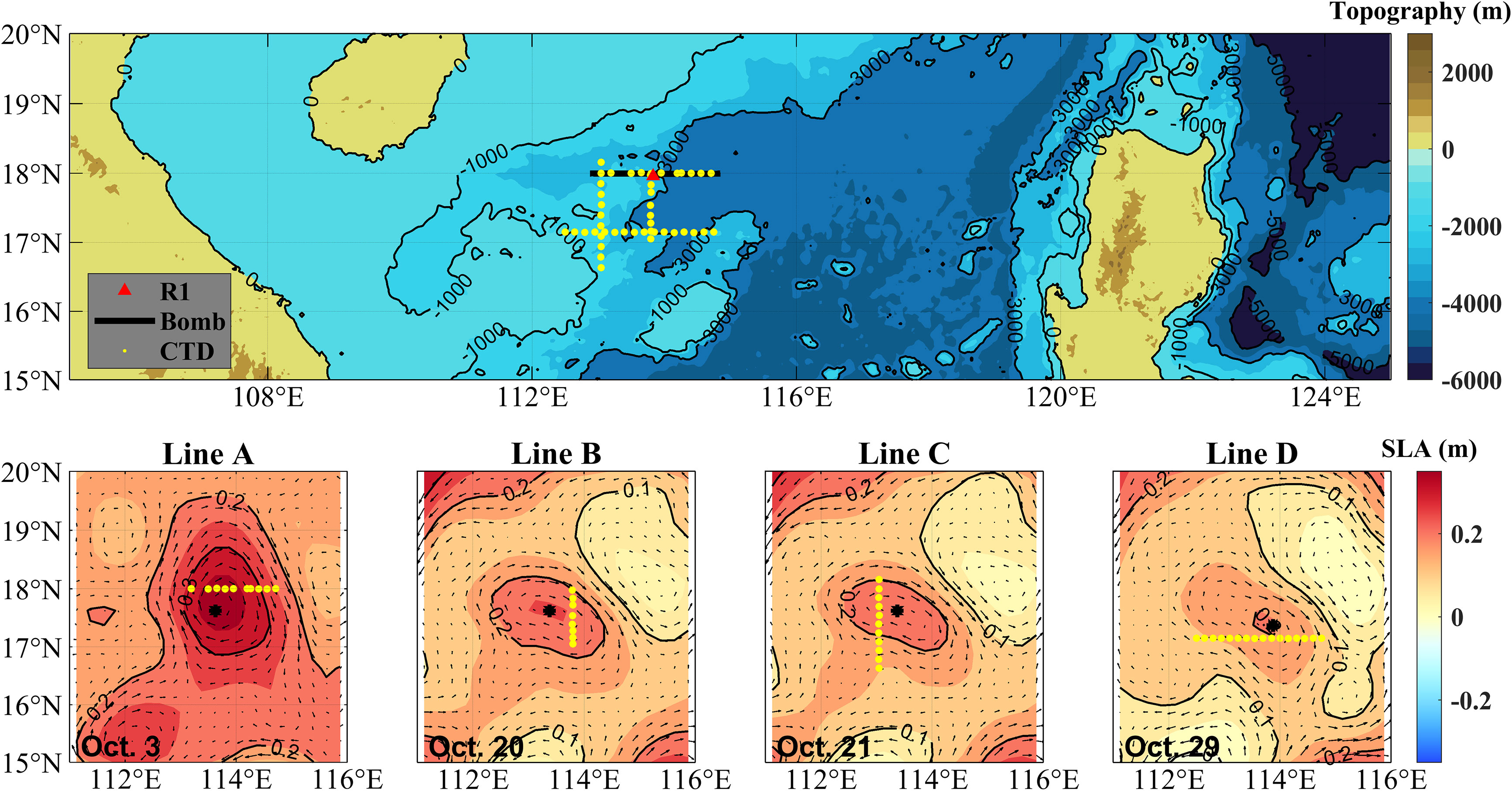
Figure 1 Map showing the environment configuration and survey stations in the EASO field experiment. The topographies (unit: m) are provided by the ETOPO2 dataset (Doi: 10.7289/V5J1012Q). The black line indicates the trajectory of explosive sound sources from the west to east. The red triangle and yellow dots indicate the vertical linear array (VLA) (marked as R1) and conductivity-temperature-depth (CTD) observation stations. The positions of the CTD observation stations are shown in the lower panel, where the shaded areas indicate the daily surface level anomalies (SLAs), and vector arrows indicate daily geostrophic currents anomalies (GCAs). According to the observation dates of CTD stations, they are named lines A, B, C and D, respectively.

2.2 Other data

2.2.1 EN.4.2.2

To obtain the eddy-induced T and S perturbations structures (hereafter referred to as eddy structure), the associated climatological profiles need to be removed. The EN.4.2.2 dataset (available at https://www.metoffice.gov.uk/hadobs/en4/download-en4-2-2.html) provides monthly mean gridded T/S profiles with a spatial resolution of 1°, which was distributed by the Met Office Hadley Center. The monthly mean gridded T/S profiles are derived from various in situ observation data like Argo floats and drifting buoys using objective analysis (Good et al., 2013).

In the field experiment, most of the observation depths of CTD are below 1500 m which is still far from the sea bottom. To calculate the sound field, the T/S profiles need to be extended to the whole depth. In this study, the EN.4.2.2 dataset is used to fill in the missing T/S data. According to the time of the EASO field experiment, the monthly T/S profiles in October 2021 are employed.

2.2.2 Sea surface anomaly

Daily sea surface level anomaly (SLA) and surface geographic current (GCA) are the critical parameters for identifying and tracking the mesoscale eddies. In the northern (southern) hemisphere, warm eddies are characterized as positive SLAs and counterclockwise (clockwise) GCAs. In the EASO field experiment, they are used to determine the CTD measurement stations located in the observed warm eddy. Additionally, the daily SLA and GCA can also reflect the variation of the position and intensity of the observed warm eddy with time.

Daily SLA and GCA with a spatial resolution of 0.25° is provided by the Copernicus Marine Environment Monitoring Service (CMEMS) with the product identifier: SEALEVEL_GLO_PHY_L4_NRT_OBSERVATIONS_008_046 (available at https://resources.marine.copernicus.eu/product-detail/SEALEVEL_GLO_PHY_L4_NRT_OBSERVATIONS_008_046/INFORMATION). The SLA was calculated by removing a twenty-year (from 1992 to 2022) mean, and gridded data was estimated by optimal interpolation.

2.2.3 ETOPO2 Dataset

As an essential bottom boundary condition for the sound propagation models, the topography profoundly affects the distribution pattern of sound energy. Especially in 3D sound propagation models, the topography is one of the most crucial factors leading to the horizontal refraction of sound rays (also called the 3D effect of sound field) compared to inhomogeneous water media (Chiu et al., 2011; Dossot et al., 2019; Liu et al., 2021b).

The ETOPO dataset merges various observation data from different measurement equipment, such as satellites, shipboard echo-sounding measurements, and so on. It provides global topography and bathymetry with different spatial resolutions, such as 0.5’, 1’ and 2’. In this work, the 2’ topography data (ETOPO2v2c, available at https://ngdc.noaa.gov/mgg/global/relief/ETOPO2/ETOPO2v2-2006/) is used to calculate the 3D sound fields in section 4.3 (different resolutions do not change the main conclusions).

2.3 Methodology

2.3.1 Ray-tracing model

To reveal the relative roles of the mesoscale eddy and topography, an acoustic propagation model is employed. Numerous sound propagation models, such as the ray-tracing model (Porter, 2019), normal mode model (Westwood et al., 1996), parabolic equation model (Collins and Werby, 1989) as well as some hybrid models are developed. Among them, the ray-tracing model is a high frequency approximation of the wave equation, which is suitable for predicting deep-sea high-frequency sound fields where the sound speeds are range-dependent. Furthermore, the ray-tracing model has a clear physical meaning, which interprets the sound field as the superposition of a series of sound rays with different propagation paths. These rays launch from the sound source to receiver points and obey the generalized Snell’s law (Porter, 2019). Considering the above factors, the ray-tracing model is employed in this study. Readers interested in detailed derivation of the ray-tracing model can refer Jensen et al. (2011).

The sound pressure calculation formula in Cartesian coordinate system is directly written as

$\begin{array}{ll}p\left(x\right)=e^{i\omega \tau \left(x\right)}\sum _{j=1}^{\infty }\frac{A_j}{{\left(i\omega \right)}^j}& (1)\end{array}$

where, $\tau \left(s\right)=\tau \left(0\right)+{\int }_0^{s}c{s}^{\prime }d{s}^{\prime }$ represents the travel time of sound ray, s′ denotes the ray trajectory, and its arclength is denoted by s. τ is derived from “Eikonal Equation” in ray coordinates. x = (x, y, z) denotes the position of the receiving point, j is the number of the sound ray, and A_j is the amplitude jth of the sound ray. c denotes the sound speed of position x, and ω denotes the angle frequency.

Bellhop and Bellhop3D, developed by Porter, 2011; Porter, 2016) are highly efficient ray-tracing programs for predicting two-dimensional (2D) and 3D acoustic pressure fields. They are used to simulating the sound field presented in section 3 and 4, and to better depict the acoustic field in shadow and caustic regions, Gaussian beam are selected in this work.

When simulating the sound fields using Bellhop and Bellhop3D, the whole-depth sound speed profiles (SSPs) of the warm eddy circumstance are necessary. Using the T, S, and depth data measured by CTD, SSPs from 0 m to 1500 m can be obtained through Mackenzie formula (Mackenzie, 1981), which is given by

$\begin{array}{ll}\begin{array}{l}c=\mathrm{1448.96 }+\mathrm{ 4.591}T-5.304\times {10}^{-2}{\text{T}}^2+2.374\times {10}^{-4}{\text{T}}^3+1.34\left(\text{S}-35\right)+1.63\times \\ {\mathrm{ 10}}^{-2}D+1.675\times {10}^{-7}{\text{D}}^2-1.025\times {10}^{-2}\left(\text{T}\times \left(\text{S}-35\right)\right)-7.139\times {10}^{-13}T{\text{D}}^3\end{array}& (2)\end{array}$

where, D indicates the depth, S and T indicate salinity and temperature, respectively.

Although the measured depth range of the CTD can cover the sound fixing and ranging (SOFAR) axis, it is still far from the local seafloor. Thus, the missing depth from 1500 m to the seafloor are filled using the climatological SSPs estimated from T and S profiles provided by the EN.4.2.2 dataset.

2.3.2 Acoustic reciprocity theorem

Figure 2 shows the experimental configuration (upper panel) and simulation conditions (lower panel), which are consistent in terms of the point-to-point acoustic response. The sound ray from S_H to RD1 (blue line) is employed to explain the acoustic reciprocity theorem (Jensen et al., 2011). In the field experiment, it is launched from the sound source S_H, which eventually undergoes the range-dependent SSPs (from No. 1 to No. n), and arrival at the receiver RD1. In the simulation, the sound ray from SD1 to R_H (blue line) travels the total opposite path. Apparently, the system responses of the above two paths are equal. Specifically, the simulation can be consistent with the experiment by swapping the positions of the sound source and receivers.

FIGURE 2

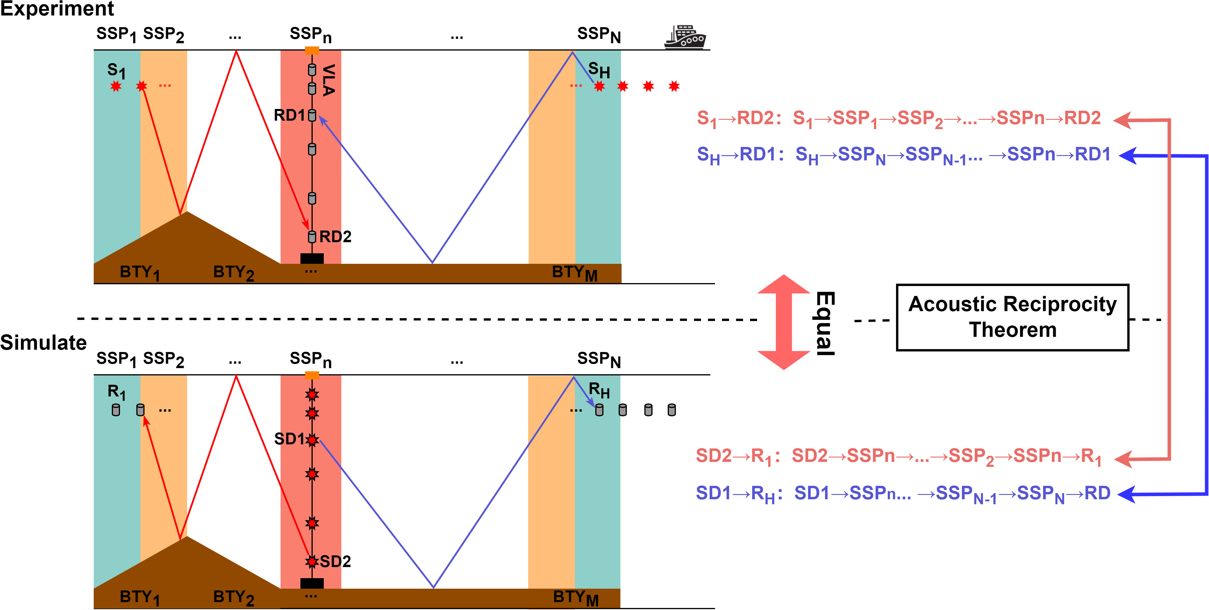
Figure 2 The diagram of acoustic reciprocity theorem of the field experiment and simulation. The upper panel shows the position of the VLA (marked with grey cylinders) and the trajectory of the explosive sound sources (marked with red eight-pointed stars) with a fixed explosive depth of 200 m. The colorful shaded areas represent range-dependent sound speeds in the presence of the warm eddy, and the brown shaded area represents the sea bottom. The red (blue) solid line indicates the sound ray launched from S₁ (S_H) and received by the RD2 (RD1) receiver. The lower panel shows the simulation configuration when analyzing the sound field using 2D and 3D ray-tracing models.

2.3.3 Processing methods of the received acoustic signals

The VLA is a type of equipment commonly used in acoustic survey experiments (Ge and Kirsteins, 2017; Song and Wang, 2022). It mainly consists of a series of hydrophones, underwater signal recorders (USR), and floats, which are combined via a Kevlar rope. The deployed depth of the hydrophone can be designed according to the experimental purpose and environment.

To obtain the transmission losses (TL) at different depths, the received signals measured by hydrophones deployed at different depths need to be processed. The specific process has been optimized into the following six steps.

Step1: Truncate the signal emitted from the sound source from the discrete time signal recorded by USR and noted as s_n = s(t_n), where s = (n − 1)Δt, (n = 1,…,N) denotes the discrete time, and n is the number of sample point. f_s denotes the sampling rate of USR and Δt = 1/f_s denotes the discrete time interval. The start time of the truncated signal can be roughly estimated from the recorded time of the bomb explosion, the horizontal distance between the sound source and the receiver, and the sound speed of the local sea water. Simultaneously, to obtain the complete signal of the explosion, the length of the window for truncating should be determined by amplitudes of recorded signals.

Step 2: Calculate the frequency spectrum of the discrete time signal s_n using Discrete Fourier Transform (DFT) method, which is written as

$\begin{array}{ll}{S}_k=\sum _{n=0}^{N=1}{s}_n\exp \left[-i\frac{2\text{π}}{N}kn\right]& (3)\end{array}$

where, k denotes the point number of the DFT.

Step 3: Calculate the total energy of the truncated signal in the 1/3 Octave frequency band of the center frequency f₀. The total energy is given by

$\begin{array}{ll}E\left(f_0\right)\approx \frac{2}{N{f}_s}\sum _{k=n_1}^{n_2}{\left|S_k\right|}^2& (4)\end{array}$

where, n₁ = f_l/d_f + 1, n₂ = f_H/d_f + 1, d_f = f_s/N. f_L = 2^−1/6f₀ and f_H = 2^1/6f₀ denote the lower and upper band of center frequency f₀.

Step 4: Compute the mean energy of the truncated signal in the narrow band from f_L to f_H. The formula is written as

$\begin{array}{ll}\widehat{E}\left(f_0\right)=\frac{1}{f_H-f_L}E\left(f_0\right)\approx \frac{2}{\left(n_2-n_1\right)f_S^2}{\displaystyle \sum _{k=n_1}^{n_2}}{\left|S_k\right|}^2& (5)\end{array}$

Step 5: Compute the source level (SL). The  SL (unit: dB) at distance R and center frequency  f₀ is given by

$\begin{array}{ll}SL\left(f_0,R\right)=10\lg \left[\widehat{E}\left(f_0\right)\right]-M_V-m+20\lg \left(R\right)& (6)\end{array}$

where, M_V denotes the sensitivity of hydrophone in dB, m denotes the magnification of the receiving system in dB, and R is the distance from source to receiver in meter.

Step 6: Calculate the TL at f₀ center frequency. TL indicates the degree of attenuation of sound energy from source to the receiver, thus, the difference between SL and $\widehat{E}\left(f_0\right)$ is the TL. The formula is given by

$\begin{array}{ll}TL\left(f_0,r\right)=SL\left(f_0\right)-\left(10\lg \left[\widehat{E}\left(f_0\right)\right]-M_V-m\right)& (7)\end{array}$

3 Analysis of observational data

3.1 Temperature and salinity structures

The surveyed eddy is accompanied with positive SLA and counterclockwise geostrophic currents as shown in Figure 1. With the evolution of SLAs in the four days, it was observed that: (1) SLAs associating with the eddy gradually decrease with time; (2) The shape of the eddy appears as an ellipse pattern changing temporally. Specifically, the long axis of the ellipse is east-west oriented at October 3, 2022, while in the other days, it becomes northwest-southeast oriented.

Based on the in-situ data measured in lines A, B, C, and D through the northern, eastern, western and southern sides of the warm eddy in Figure 1 (yellow dots), the corresponding T, temperature anomaly (TA), S, salinity anomaly (SA), density (Den), and density anomaly (DA) vertical sections of the eddy are exhibited in Figure 3, respectively. Following the naming rules of CTD lines in Figure 1, the four vertical sections here are also named sections A, B, C, and D, respectively. Among them, T and S are directly measured by CTD observation stations, Den is derived from T, S and pressure, and the TA, SA and DA are computed by removing the associated climatological profile provided by the EN.4.2.2 dataset.

FIGURE 3

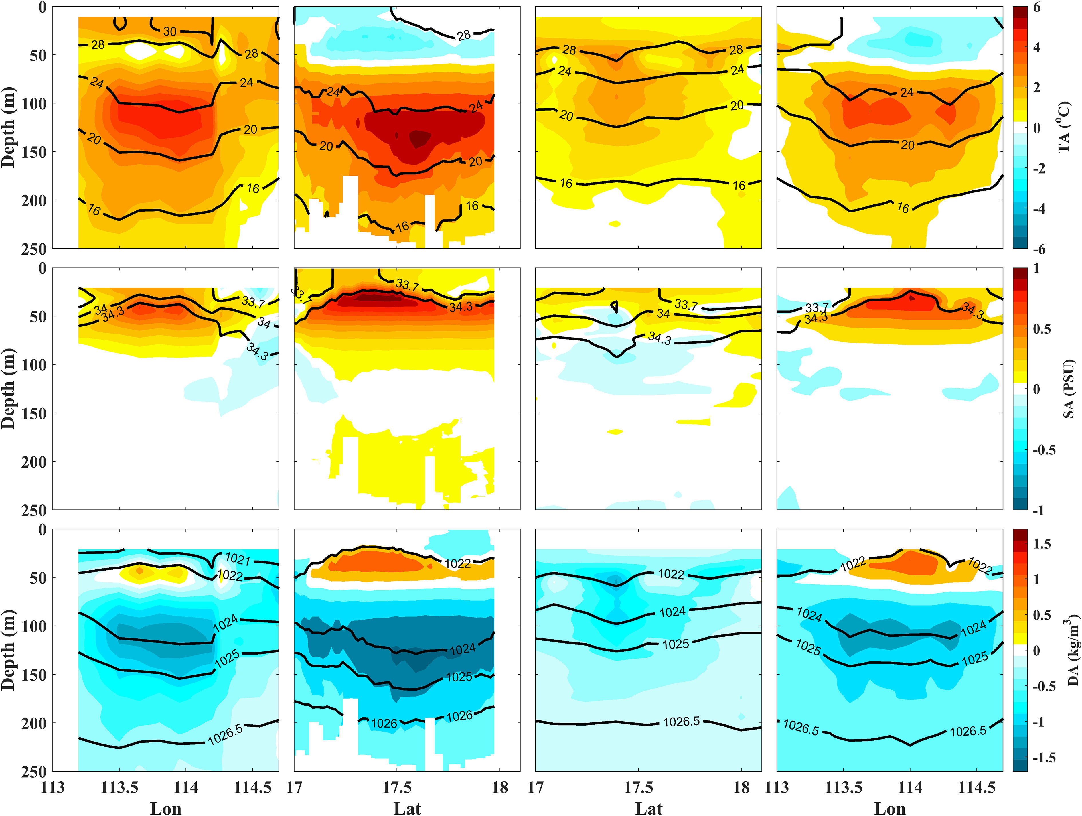
Figure 3 The four investigated thermohaline vertical sections of the warm eddy measured by A, B, C and D from left to right, respectively. The T (unit: °C) structures of the investigated vertical sections are shown in upper panels, where the shaded areas show the magnitude of TA (unit: °C), and the solid black lines indicate isotherms. The S (unit: PSU) structures of the investigated vertical sections are shown in middle panels; the shaded areas show the magnitude of SA (unit: PSU), and the solid black lines indicate iso-salinity lines. The Den (unit: kg/m³ ) structures of the investigated vertical sections are shown in bottom panels; the shaded areas show the magnitude of DA (unit: kg/m³), and the solid black lines indicate isopycnal lines. The x-axis indicates latitudinal and longitudinal ranges. The y-axis indicates the water depth from 0 m to 250 m.

Through the distributions of SAs and TAs in the four vertical sections, it was observed that the eddy-induced TA and SA occur at different depths. The TA is confined to the depths from 70 m to 200 m with a maximum TA of about 6^∘C, while the SA is confined to the depths from 10 m to 70 m with a maximum SA of about 1 PSU. Simultaneously, isohalines and isotherms of the warm eddy exhibit lenticular structures with an upper convexity and a lower concavity, respectively. Based on the T and S characteristics accompanied with the SLAs, it was concluded that it is a surface-intensified warm eddy (Chaigneau et al., 2011).

There are different behaviors among the four vertical sections, indicating significant differences in terms of SA and TA structures at different times and positions of the warm eddy. Specifically, the dipole structures of TA are demonstrated in vertical sections B and D, where the cold and warm cores occur at depths of about 40 m and 130 m, respectively. Similar to the TA, DAs in vertical sections, B and D also show dipole structures. On the contrary, the monopole structures of TA are demonstrated in vertical sections A and C with warm core depths of 120 m and 50 m, respectively.

The measurement of vertical sections B and C were conducted in two consecutive days (Oct 20 and 21, respectively), of which the difference in measurement times is negligible relative to the slow propagation of the mesoscale eddy. Therefore, it is reasonable to use vertical sections B and C to represent the structures at different positions of the eddy at the same moment. Further, the difference between vertical sections B and C can prove that the western and eastern sides of the eddy are still significantly different in T and S structures even simultaneously. For instance, on the western side of the eddy (section C), the TA is small, and even a slight negative SA (-0.18 PSU) appears in the center of the TA. While on the eastern side of the eddy (section B), the most significant positive TA (6°C) and SA (1 PSU) are observed.

By comparing the SLAs in Figure 1 and subsurface anomalies (Figure 3) associated with the four vertical sections, it shows that the subsurface features could reflect the surface characteristics. For instance, the upraising (negative) and depressing (positive) of isopycnal lines (SLA) basically follow the first-order baroclinic mode relationship.

As mentioned in Section 2.1, a total of 105 CTD station observations were performed during the entire EASO field experiment. Among them 55 CTD (not shown), from October 20 to October 30, 2021, are selected to composite the 3D structure of the observed eddy. As shown in Figure 1, SLAs and GCAs demonstrate that the surface shape and position of the eddy had moderate changes during that period. Thus, the corresponding gridded observation stations are selected to composite the 3D structure, which are sufficient to represent the impact of the eddy on the sound propagation. Using all the 105 stations will not change the main conclusions of the study (figures not shown).

After interpolating the T and S observations of 55 CTD stations onto the 3D grid points, the 3D T and S structures of the warm eddy are obtained, as shown in Figures 4A, B. The 3D TA and SA structures in Figures 4C, D are obtained by removing the associated climatological profile provided by the EN4.2.2 dataset from the 3D T and S of the eddy, respectively. From 110 m to 170 m depths, the shapes of T and TA show good consistency with the surface shape of the eddy defined by the contour of SLA. As shown in Figure 1, from October 20 to October 30, 2021, the shape of the eddy at the surface is ellipse-like, with the long axis of the ellipse-oriented northwest-southeast. Simultaneously, the shapes of T and TA also exhibit elliptical patterns, with the long axis of the ellipse oriented in the same direction as that of the surface. Furthermore, the composited 3D eddy maintains the features in core depths of TA and SA, which are confined in 70 m to 200 m and 10 m to 70 m, respectively. The composited 3D eddy here will support the study of its 3D sound field in section 4.3.

FIGURE 4

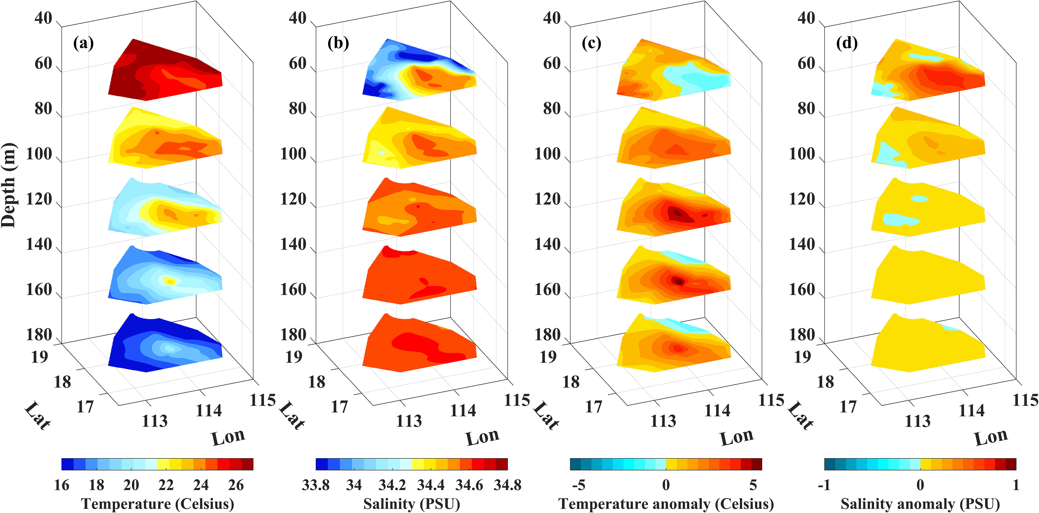
Figure 4 3D structures of the warm eddy. The (A) T (unit: °C), (B) S (unit: PSU), (C) TA (unit: °C), and (D) SA (unit: PSU) slices at depths from 50 m to 170 m with an interval of 30 m are shown from left to right panels.

3.2 Acoustic characteristics

Figure 5 (right panel) illustrates the whole-depth vertical section of SSPs associated with line A, as well as the acoustic survey line, where the R1(VLA) is arranged at 0 km, and the x-axis is eastward. The black solid lines indicate the eddy-induced density anomalies. Simultaneously, bathymetries measured by the shipboard echo sounders are shown in Figure 5, agreeing well with the bathymetries provided by the ETOPO2 dataset (Figure 1, upper panel). Furthermore, to exhibit impacts of the warm eddy, SSPs in the warm eddy (red line) and none eddy (blue dots) circumstances are also presented in Figure 5 (left panel). The impacts of the warm eddy on sound speeds are indicated by the red shallow area. The SSP in the eddy center is marked with the white dotted line in Figure 5 (right panel); while the SSP representing the none eddy case selected from the monthly mean SSP is located at the same position. Obviously, both the two SSPs in Figure 5 are incomplete sound channel environments due to the local bathymetries.

FIGURE 5

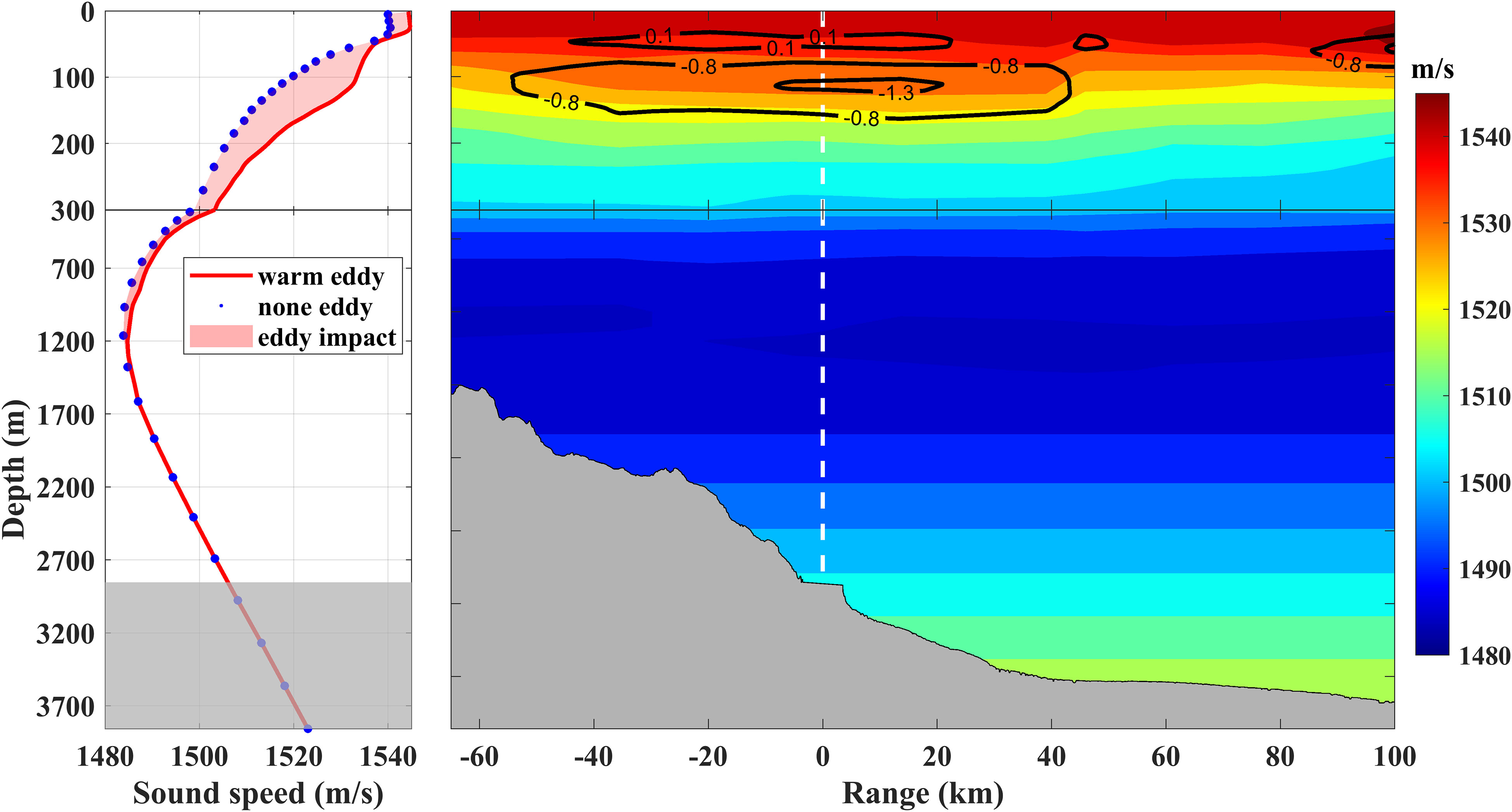
Figure 5 Sound speed (unit: m/s) of the section A. The SSPs in warm eddy (red solid line) and none eddy (blue dotted line) circumstances are shown in the left panel, and the red shadow area indicates the impacts of the warm eddy on sound speeds. The 2D sound speed distribution is shown in the right panel, an the black solid lines represent the anomalies of density induced by the warm eddy. The white dotted line indicates the position of VLA (R1), where SSP corresponds to the red one in the left panel.

Some differences between the warm eddy SSP and none eddy SSP were observed, illustrated by the following aspects: (1) The warm eddy leads to a higher T in the upper layer. Thus, the value at the surface of the warm eddy SSP (1544 m/s) is slightly faster than that of none eddy SSP (1540 m/s). (2) The warm eddy SSP shows two rapid vertical changes from 29 m to 45 m and from 115 m to 300 m depths. (3) The impact of the surface-intensified eddy is mainly concentrated at the depths from 0 m to 300 m, and the most significant difference between the warm eddy SSP and none eddy SSP is about 15 m/s occurring at a depth of 135 m. In depths deeper than 135 m, the difference in sound speed caused by the warm eddy gradually decreases and disappears at a depth of 1200 m, which is close to the SOFAR axis. In terms of the vertical section of sound speed, iso-speed lines show a downward concave pattern within the warm eddy and gradually lift as moving to both sides of the eddy center.

Through the processing procedure mentioned in Section 2.3.3, the TL curve at the receiving depth (RD) of 185 m and 300 Hz center frequency for the EASO field experiment is presented in the bottom panel of Figure 6, marked with black cross symbols. For the R1-T2 survey line, two obvious CZs with about 70 dB and 78 dB TL at about 39 km and 92 km, respectively, were observed. As for the T1-R1 survey line, only a CZ with about 72 dB TL at about -25 km influenced by the rough topographies was observed.

FIGURE 6

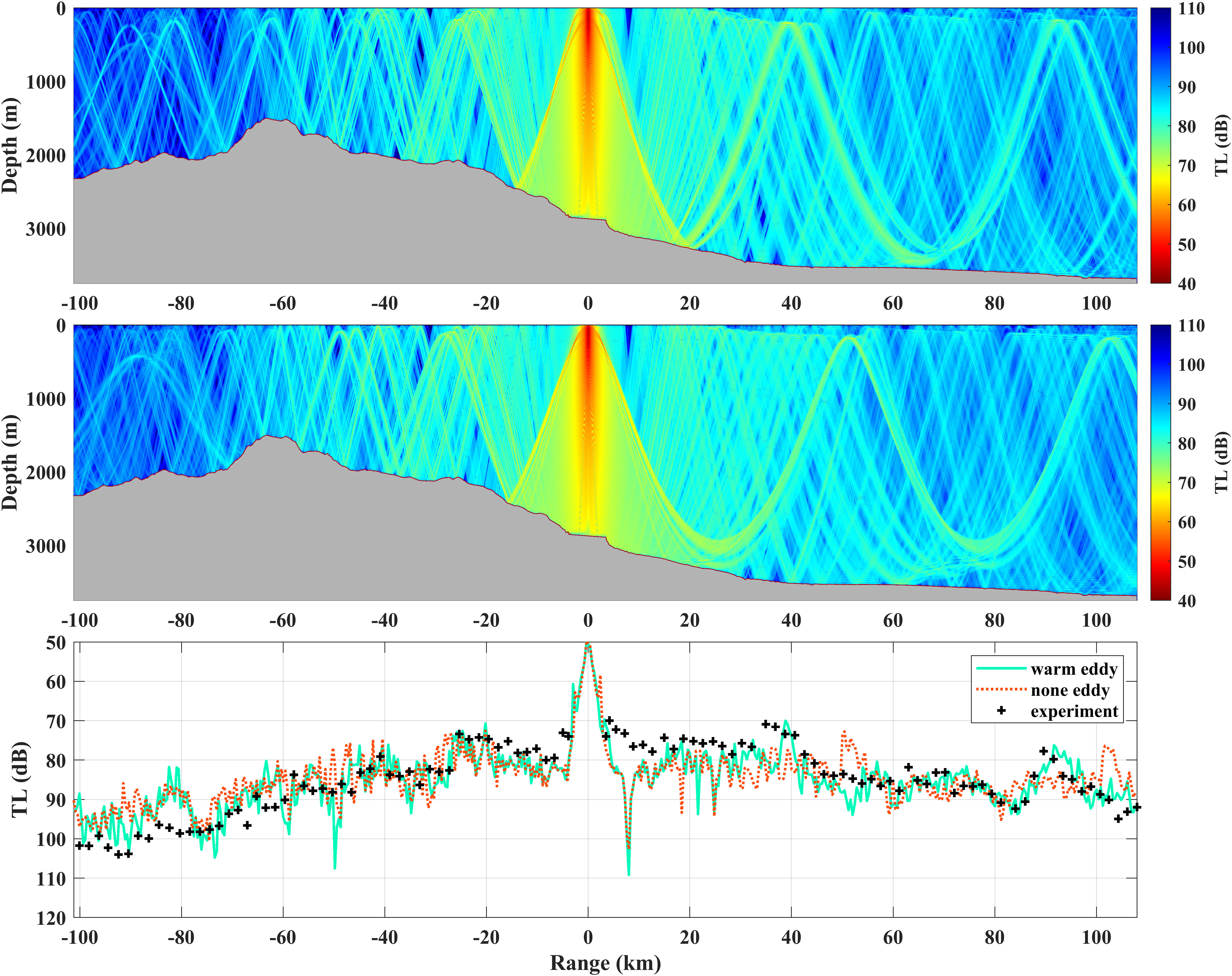
Figure 6 The comparison of sound field between the warm eddy and none eddy circumstances. The 2D sound TL in the r-z plane with warm eddy (none eddy) circumstance is shown in the upper (middle) panel, where the source is deployed at 185 m depth and 0 km distance, and the grey shaded area represent the sea bottom. The TL (unit: dB) curves are arranged in the bottom panel with the fixed RD of 200 m. The green solid line, red dotted line, and black cross symbols indicate the TLs for the simulated warm eddy, simulated none eddy, and in the experiment, respectively.

4 Discussion

4.1 Comparisons of sound fields between warm eddy and none eddy circumstances

To analyze the acoustic experiment, the simulations based on the acoustic reciprocity theorem with Bellhop (Porter, 2011) are performed. As shown in Figure 6 (top panel), the simulated 2D TL with the warm eddy circumstance is computed within the narrow band determined by the 1/3 octave of the center frequency of 300 Hz, where the simulated sound source is set at a depth of 185 m. The coherent Gaussian Beams are employed in Bellhop. The acoustic absorption coefficient of the water body dominated by frequency can be estimated with the following formula (Jensen et al., 2011), written as

$\begin{array}{ll}\text{α}=3.3\times {10}^{-3}+\frac{0.11f^2}{1+f^2}+\frac{44f^2}{4100+f^2}+3.0\times {10}^{-4}{f}^2& (8)\end{array}$

where, f denotes frequency in kHz, and the unit of α is dB/km. Due to the incomplete sound channel, sound rays frequently interact with the sea floor. Therefore, the acoustic absorption coefficient of the local sea floor is a crucial parameter. However, there are no sediment observations in the EASO field experiment. Thus, it is represented by a fixed value of 0.2 dB/wavelength. As shown in Figure 6 (bottom panel), there is a good consistency between the simulated (Figure 6, green line) and experiment TL curves in the presence of the warm eddy.

From the simulated 2D TL (Figure 6, top panel) with the warm eddy circumstance, the possible causes for the difference between TL curves of T1-R1 and R1-T2 can be determined. The topographies in R1-T2 are flatter and deeper, in favor of the formation of CZs. Contrarily, topographies in T1-R1 are rougher and shallower, leading to the high-frequency interaction between sound rays and sea floors, and thus destroy the structure of the CZ.

To demonstrate the effect of warm eddy on the sound field, the simulated TL results (Figure 6, middle and bottom panels) with the none eddy circumstance are calculated as a comparison, where the simulation conditions are the same as that in the warm eddy circumstance except for the range-independent SSP (the blue dotted line in Figure 5) deriving from the EN.4.2.2 dataset through Formula (2). From the 2D sound field of the none eddy case in R1-T2, it was observed that two CZs at about 50.4 km and 101.7 km are present. As for the T1-R1 line, only one CZ with about 72 dB TL at about -25 km is present.

By comparing the TL curves with and without eddy (red dotted line) in R1-T2, it was observed that the first and second CZs in the warm eddy case exhibit noticeable forward shifts with about 11.4 km and 9.7 km, respectively. However, in the T1-R1 survey line, it is hard to find obvious difference in CZs. Additionally, the differences in sound fields between the two circumstances are also manifested in the depth and width variations of the CZ. As shown in Figure 6 (upper panel), the second CZ (150 m) shows a downward lifting of about 32 m compared to that of the first (182 m), while such a phenomenon cannot be found in the none eddy case. In the warm eddy case, the widths of the first and second CZs are 10.4 km and 9 km, respectively, showing a change of 1.4 km.

4.2 Roles of topography and eddy

In this section, the respective roles of topography and warm eddy in changing sound fields will be discussed. Figure 6 shows that both the warm eddy and topography are responsible for the differences in sound fields between warm eddy and none eddy circumstances. In the T1-R1 survey line, the rough and shallow topographies result in the frequent interaction between sound rays and the bottom, and thus obscure the effects of the warm eddy on sound rays, which render the differences in TL curves imperceptible. Contrarily, in the R1-T2 survey line, the sound rays only hit the relatively flat and deep bottom one time before the first CZ in the warm eddy circumstance. Between the first and second CZs, the sound rays only experienced the refraction of the warm eddy-induced water body. Therefore, the fields before and after the first CZ in the R1-T2 survey line can illustrate the impacts of the warm eddy and topography on sound fields, respectively.

The sound ray traces simulated by Bellhop are presented to further interpret the differences between the warm eddy (upper panel) and none eddy (lower panel) circumstances in the R1-T2 line, as shown in Figure 7. Here, different coloured lines are used to identify purely refracted paths that do not hit surface and bottom boundaries (black), one bottom-reflected paths (red), more than one bottom-reflected paths (green), and both surface and bottom paths (blue), respectively.

FIGURE 7

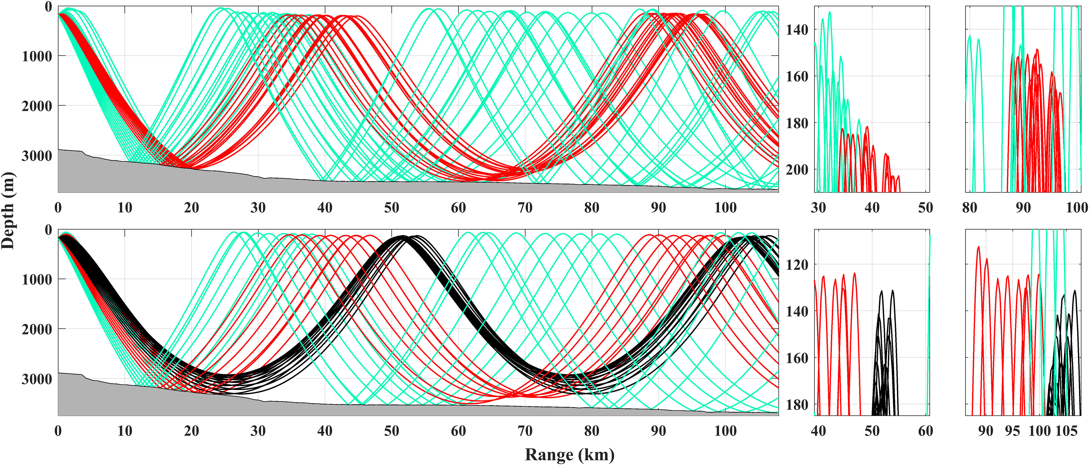
Figure 7 The comparison of simulated sound ray traces with 300 Hz frequency between the warm eddy (upper panel) and none eddy (lower panel) circumstances. The two right columns show the enlarged and detailed characteristics.

Considering the relative roles of topography and warm eddy on the horizonal span of CZs, as shown in Figure 7 (upper panel), in the warm eddy circumstance, the sound rays launched from source and hit the bottom one time and then generate the first CZ in 39 km. Thereafter, the bottom-reflected sound ray only experienced refraction and generate the second CZ in 92 km. In the none eddy circumstance, both the first (50.4 km) and second CZs (101.7 km) are mainly generated by the purely refracted rays (black lines), representing the fields avoiding the influence of the topography and warm eddy. Thus, the differences in the horizontal spans of the two CZs between the warm and none eddy circumstances represent the influences dominated by the topography and warm eddy, respectively. The comparison results indicate that the topography shortens the horizontal span of the CZ by 11.4 km, while the warm eddy lengthens it by 1.7 km.

Considering the impact of warm eddy on the vertical shift of CZ, as only the warm eddy impacts the sound rays between the first and second CZs in the warm eddy circumstance, the difference between the first and second CZ can directly reflect the effect of the warm eddy. As shown in the detailed views of Figure 7 (upper panel), the first and second CZs are at depths of 182 m and 150 m, showing an upward vertical shift of about 32 m resulting from the warm eddy. As the first CZ is close to the center of the warm eddy, it can be concluded that the depth of the CZ decreases as it moves away from the center of the warm eddy. Specifically, the warm eddy decreases the depth of the CZ. Considering the impact of warm eddy on the width of CZ, from the detailed views of Figure 7 (upper panel), it was observed that the widths of the first and second CZs are 10.4 km and 9 km, respectively, showing a decrease of about 1.4 km. The comparison results indicate that the width of the CZ decreases as moving away from the center of the warm eddy. Specifically, the warm eddy increases the width of the CZ.

To provide more insights into the sound field impacted by the warm eddy, the arrival structures and travel times of rays at the first (39 km) and second CZs (92 km) with warm eddy (left panels) and none eddy (right panels) circumstances are presented in Figure 8. It was observed that travel times in the warm eddy case are shorter than those in the none eddy case due to the higher sound speed induced by the warm eddy. Additionally, the arrival structure of the second CZ in the warm eddy case is more complex than that in the none eddy case.

FIGURE 8

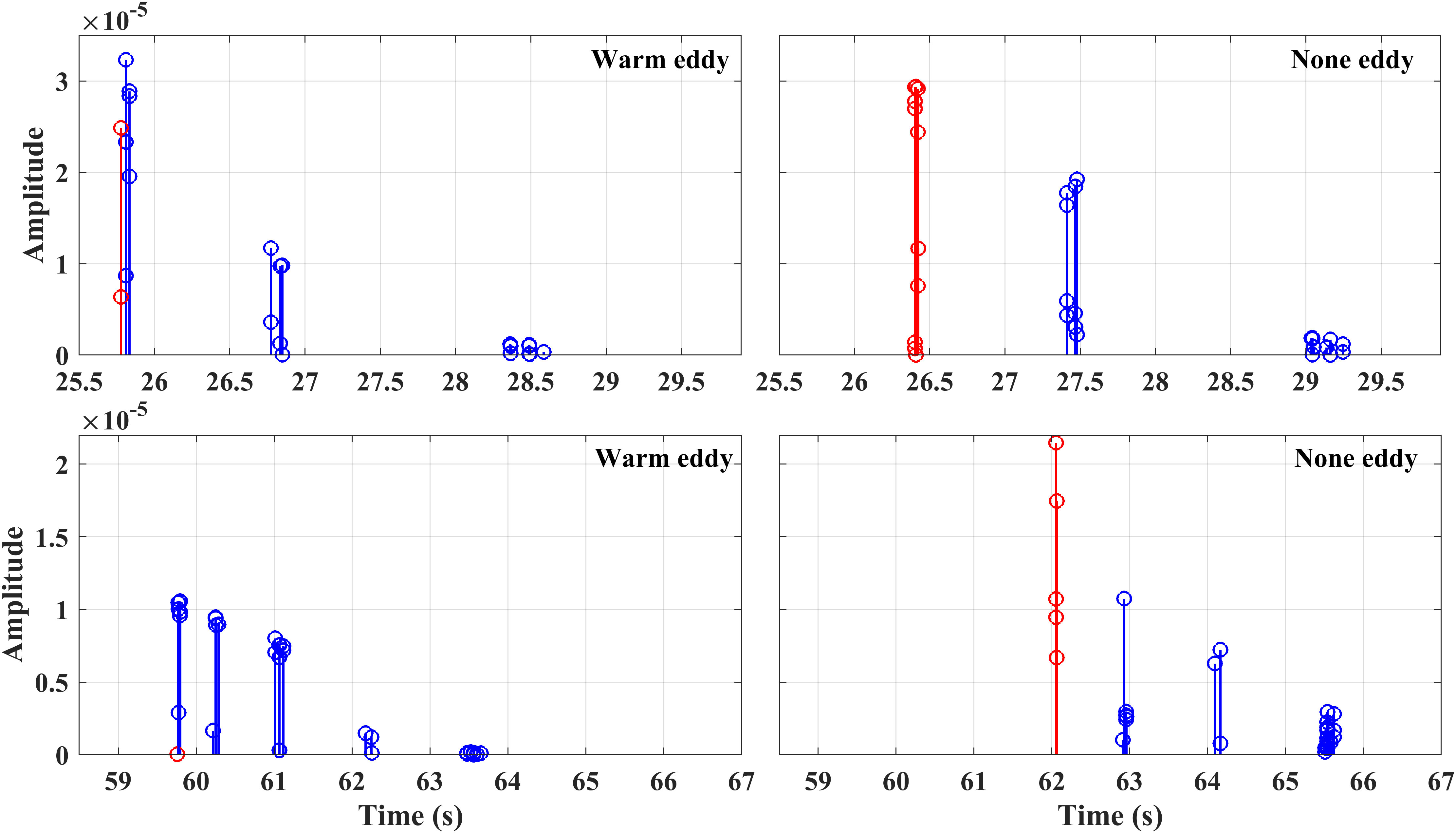
Figure 8 Arrivals from the sound source at 185 m depth and 0 km distance to the receiver at 200 m depth and 39 km (upper panel) and 92 km (lower panel) distances with warm eddy (left panel) and none eddy (right panel) circumstances.

4.3 3D Effects of the warm eddy on sound fields

In the incomplete sound channel environment, both SSPs and topographies should be taken into consideration for predicting the sound field. To study the anisotropy of the 3D sound field jointly dominated by the eddy and topographies, the 3D sound field calculated with the Bellhop3D (Porter, 2011) in the receiving depths of 20 m, 200 m, 1000 m, and 2000 m are illustrated (Figure 9). In Figure 9, the Cartesian coordinate system is transformed from the earth coordinate system originating at 16.5°N, 112°E, and the eastward x-axis and northward y-axis denote latitudinal and longitudinal ranges, respectively.

FIGURE 9

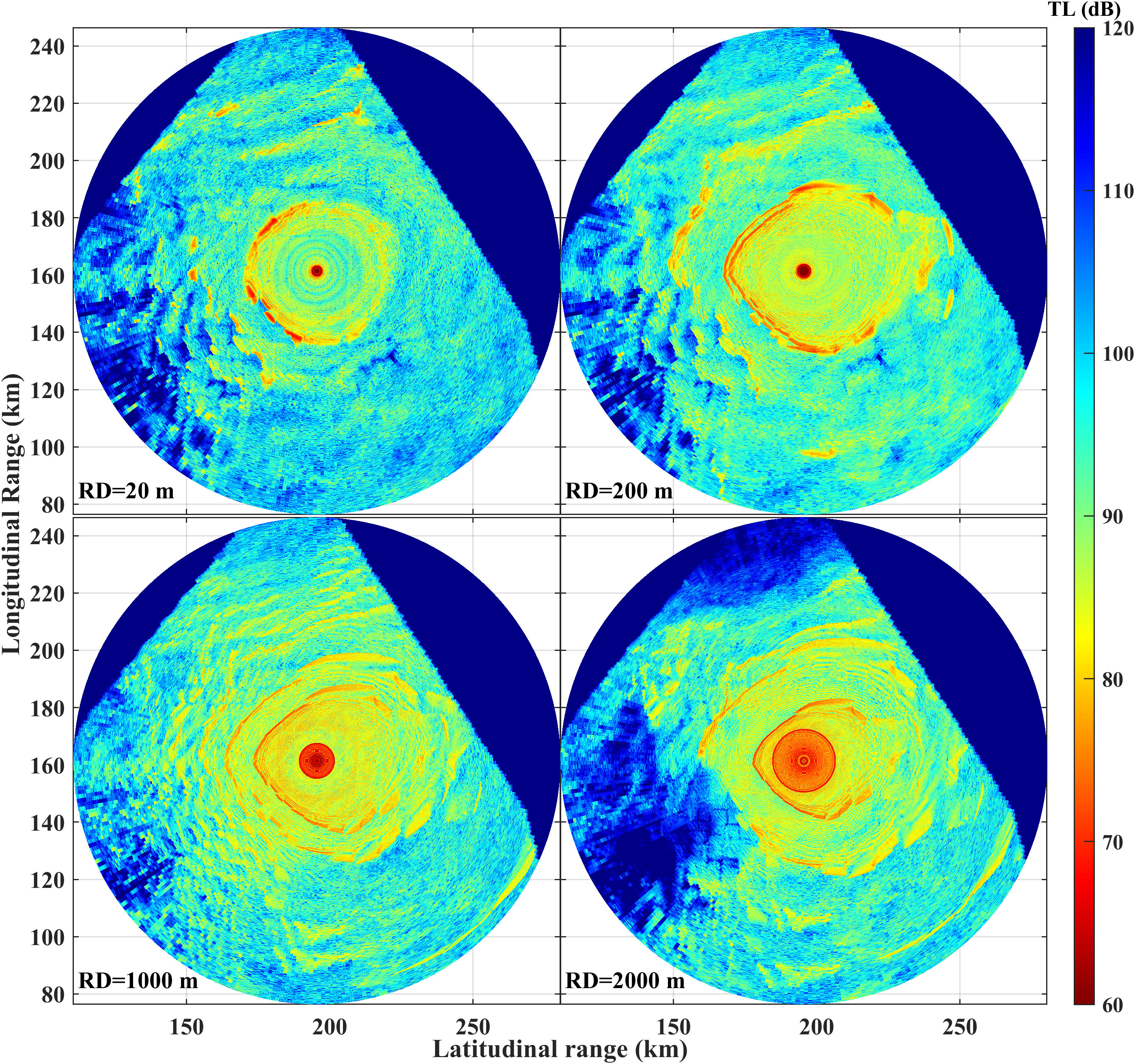
Figure 9 The 3D sound field at cartesian coordinate system in the presence of warm eddy and complex topography. The sound source is deployed at 195.5 km, 161.4 km, and 0.185 km with 300 Hz frequency. Top views of the TLs at receiver depths of 20 m, 200 m, 1000 m and 2000 m are shown, respectively.

The 3D sound speed of the warm eddy is derived from the 3D T and S from Figures 4A, B through Formula (2), and the 3D topography is provided by the ETOPO2 dataset. The sound source is deployed at 195.5 km, 161.4 km, and 0.185 km with 300 Hz frequency. Additionally, the azimuth angle in horizontal plane is set from 0° (eastward) to 360° with an interval of 1°, and the pitch angle in vertical plane is set from -180° (downward) to 0° with an interval of 1°. The acoustic survey line T1–T2 corresponds to the line parallel to the x-axis and passing through the source.

From the simulation results, it was observed that all the first CZs are the reflection type, which implies that the topography is the primary factor determining the sound field, while the warm eddy-induced 3D sound speed field is the second factor. By comparing the sound fields in the mixed layer (20 m) and the thermocline (200 m), it is found that there are significant differences in the distribution patterns of sound fields. In the mixed layer, the distances of the first CZs are relatively uniform. But in the thermocline, the distances of the first CZs exhibit significant non-homogeneous. For the first reflection CZ, its horizontal distance to the source increases with the depth of the seafloor. For the TLs at a depth of 200 m, the CZs positions vary with the horizontal propagation directions, which are referred to as the anisotropy of the sound field. Specifically, the distances of the first CZs on the eastern side of the sound source are longer than that on the western side. The nearest (20 km) and farthest (51 km) CZs occur in the 213° and 15° directions of the sound source, respectively, which correspond to the rough and flat topographies in the study area. Furthermore, in the 3D sound fields, the most significant shadow zones induced by the rough and shallow topography, with most TLs higher than 110 dB, are observed in the southwest and northwest corners at a depth of 2000 m.

5 Conclusions

An eddy-acoustic synchronous observation field experiment was performed in the slope of the South China Sea in October, 2021, to study the effects of the warm eddy on sound fields. A total of 105 CTD profiles and an acoustic survey line with about 210 km length are measured in the experiment. In the hydrological part of the investigation, four complete vertical sections precisely crossing the northern, southern, eastern and western sides of the center of the observed warm eddy were present. From the four vertical sections of the eddy, the lenticular structures of isohalines and isotherms were observed. The subsurface and surface characteristics suggested that the observed warm eddy is surface-intensified and ellipse-like in shape. Subsequently, 55 CTD profiles were chosen to composite the 3D structures of the observed eddy, which showed consistent structures with surface and the largest TA and SA distributing in 70 m to 200 m and 10 m to 70 m, respectively.

In the acoustic part of the experiment, the acoustic observation showed the presence of two obvious CZs at about 39 km and 92 km in R1-T2 line with flatter and deeper bottom, and one CZ at about 25 km in T1-R2 with rough and shallower bottom, indicating that the topography and warm eddy are jointly responsible for the differences. To quantitatively analyze the acoustic behaviors of the topography and warm eddy, a ray-tracing acoustic model is adopted to compare the sound fields with and without eddy circumstances, as well as the different topographies. The comparison results showed that the topography shortens the horizontal span of the CZ by 11.4 km, while the warm eddy lengthens it by 1.7 km. Additionally, the warm eddy decreases the depth of the CZ by 32 m, and increases its width 1.4 km. Finally, based on the composited 3D eddy, anisotropy of 3D sound fields is found through Bellhop3D. The results show that the distances differences of the first CZs in different horizontal directions can be up to 31 km.

The effects of topographies on the sound field, such as the submarine mountain, slop, and ridge, were widely studied in the traditional acoustical works, suggesting that topography has the most significant effect on the sound field (Chiu et al., 2011; Dossot et al., 2019; Liu et al., 2021b). However, the effects of inhomogeneous water bodies were not discussed thoroughly in these studies due to the complicated oceanic processes. In this study, benefiting from the well-designed field experiment, quantitative effects of the topography and warm eddy are obtained. In future works, the topography-induced horizontal refraction effects in the sound fields will be emphasized on different oceanic systems, such as fronts, internal waves, sub-mesoscale processes, and so on.

Data availability statement

The original contributions presented in the study are included in the article/supplementary material. Further inquiries can be directed to the corresponding authors.

Author contributions

WC performed the data analysis and wrote the initial draft. YCZ proposed the main ideas and dramatically modified the manuscript. YL and KR all participated in the discussion and contributed to the improvement of the manuscript. All authors contributed to the article and approved the submitted version.

Funding

This work is supported by the Science and Technology Innovation Program of Hunan Province (2022RC3070) and the National Natural Science Foundation of China under Grant No. 62101578.

Acknowledgments

The authors thank all of the experiment participants for their great efforts to make this experiment successful in 2021. The authors thank Wei Guo and Guojun Xu for their reasonable advices on acoustic calculation.

Conflict of interest

The authors declare that the research was conducted in the absence of any commercial or financial relationships that could be construed as a potential conflict of interest.

Publisher’s note

All claims expressed in this article are solely those of the authors and do not necessarily represent those of their affiliated organizations, or those of the publisher, the editors and the reviewers. Any product that may be evaluated in this article, or claim that may be made by its manufacturer, is not guaranteed or endorsed by the publisher.

References

Baer R. N. (1981). Propagation through a three-dimensional eddy including effects on an array. J. Acoust. Soc Am. 69 (1), 70–75. doi: 10.1121/1.385253

CrossRef Full Text | Google Scholar

Calado L., Gangopadhyay A., da Silveira I. C. A. (2006). A parametric model for the Brazil current meanders and eddies off southeastern Brazil. Geophys. Res. Lett. 33 (12), L12602. doi: 10.1029/2006GL026092

CrossRef Full Text | Google Scholar

Chaigneau A., Le Texier M., Eldin G., Grados C., Pizarro O. (2011). Vertical structure of mesoscale eddies in the eastern south pacific ocean: A composite analysis from altimetry and argo profiling floats. J. Geophys. Res.: Oceans. 116 (C11), C11025. doi: 10.1029/2011JC007134

CrossRef Full Text | Google Scholar

Chelton D. B., Schlax M. G., Samelson R. M. (2011). Global observations of nonlinear mesoscale eddies. Prog. Oceanogr. 91 (2), 167–216. doi: 10.1016/j.pocean.2011.01.002

CrossRef Full Text | Google Scholar

Chen C., Jin T., Zhou Z. (2019). Effect of eddy on acoustic propagation from the surface duct perspective. Appl. Acoust. 150, 190–197. doi: 10.1016/j.apacoust.2019.02.019

CrossRef Full Text | Google Scholar

Chen W., Zhang Y., Liu Y., Ma L., Wang H., Ren K., et al. (2022). Parametric model for eddies-induced sound speed anomaly in five active mesoscale eddy regions. J. Geophys. Res.: Oceans. 127 (8), e2022JC018408. doi: 10.1029/2022JC018408

CrossRef Full Text | Google Scholar

Chiu L. Y. S., Lin Y.-T., Chen C.-F., Duda T. F., Calder B. (2011). Focused sound from three-dimensional sound propagation effects over a submarine canyon. J. Acoust. Soc Am. 129 (6), EL260–EL266. doi: 10.1121/1.3579151

PubMed Abstract | CrossRef Full Text | Google Scholar

Collins M. D., Werby M. F. (1989). A parabolic equation model for scattering in the ocean. J. Acoust. Soc Am. 85 (5), 1895–1902. doi: 10.1121/1.397896

CrossRef Full Text | Google Scholar

Colosi J. A., Cornuelle B. D., Dzieciuch M. A., Worcester P. F., Chandrayadula T. K. (2019). Observations of phase and intensity fluctuations for low-frequency, long-range transmissions in the Philippine Sea and comparisons to path-integral theory. J. Acoust. Soc Am. 146 (1), 567–585. doi: 10.1121/1.5118252

PubMed Abstract | CrossRef Full Text | Google Scholar

Dossot G. A., Smith K. B., Badiey M., Miller J. H., Potty G. R. (2019). Underwater acoustic energy fluctuations during strong internal wave activity using a three-dimensional parabolic equation model. J. Acoust. Soc Am. 146 (3), 1875–1887. doi: 10.1121/1.5125260

PubMed Abstract | CrossRef Full Text | Google Scholar

Gao F., Xu F.-H., Li Z.-L. (2022). The effects of mesoscale eddies on spatial coherence of middle range sound field in deep water. Chinese. Phys. B 31 (11). doi: 10.1088/1674-1056/ac6014

CrossRef Full Text | Google Scholar

Ge H., Kirsteins I. P. (2017). Characterization and exploitation of lucky scintillations in HLA and VLA data from the 2006 shallow water experiment. J. Acoust. Soc Am. 141 (5), 3918–3918. doi: 10.1121/1.4988853

CrossRef Full Text | Google Scholar

Good S. A., Martin M. J., Rayner N. A. (2013). EN4: Quality controlled ocean temperature and salinity profiles and monthly objective analyses with uncertainty estimates. J. Geophys. Res.: Oceans. 118 (12), 6704–6716. doi: 10.1002/2013JC009067

CrossRef Full Text | Google Scholar

Henrick R. F., Siegmann W. L., Jacobson M. J. (1977). General analysis of ocean eddy effects for sound transmission applications. J. Acoust. Soc Am. 61 (S1), S11–S11. doi: 10.1121/1.2015408

CrossRef Full Text | Google Scholar

Jensen F. B., Kuperman W. A., Porter M. B., Schmidt H., Tolstoy A. (2011). Computational ocean acoustics (Springer).

Google Scholar

Jian Y. J., Zhang J., Liu Q. S., Wang Y. F. (2009). Effect of mesoscale eddies on underwater sound propagation. Appl. Acoust. 70 (3), 432–440. doi: 10.1016/j.apacoust.2008.05.007

CrossRef Full Text | Google Scholar

Liu J., Piao S., Gong L., Zhang M., Guo Y., Zhang S. (2021a). The effect of mesoscale eddy on the characteristic of sound propagation. J. Mar. Sci. Eng. 9 (8). doi: 10.3390/jmse9080787

CrossRef Full Text | Google Scholar

Liu W., Zhang L., Wang W., Wang Y., Ma S., Cheng X., et al. (2021b). A three-dimensional finite difference model for ocean acoustic propagation and benchmarking for topographic effects. J. Acoust. Soc Am. 150 (2), 1140–1156. doi: 10.1121/10.0005853

PubMed Abstract | CrossRef Full Text | Google Scholar

Mackenzie K. V. (1981). Nine-term equation for sound speed in the oceans. J. Acoust. Soc Am. 70 (3), 807–812. doi: 10.1121/1.386920

CrossRef Full Text | Google Scholar

Nan F., Yu F., Wei C., Ren Q., Fan C. (2017). Observations of an extra-Large subsurface anticyclonic eddy in the northwestern pacific subtropical gyre. J. Mar. Sci. Res. Dev. 7, 234. doi: 10.4172/2155-9910.1000234

CrossRef Full Text | Google Scholar

Porter M. B. (2011) The BELLHOP manual and user’s guide PRELIMINARY DRAFT. Available at: http://oalib.hlsresearch.com/Rays/HLS-2010-1.pdf.

Google Scholar

Porter M. B. (2016) Bellhop3D user guide. Available at: https://usermanual.wiki/Document/Bellhop3D20User20Guide202016725.1524880335/view.

Google Scholar

Porter M. B. (2019). Beam tracing for two- and three-dimensional problems in ocean acoustics. J. Acoust. Soc Am. 146 (3).2016 doi: 10.1121/1.5125262

PubMed Abstract | CrossRef Full Text | Google Scholar

Ramp S. R., Colosi J. A., Worcester P. F., Bahr F. L., Heaney K. D., Mercer J. A., et al. (2017). Eddy properties in the subtropical countercurrent, Western Philippine Sea. Deep. Res. Part I Oceanogr. Res. Pap. 125, 11–25. doi: 10.1016/j.dsr.2017.03.010

CrossRef Full Text | Google Scholar

Song W., Wang P. (2022). High-resolution modal wavenumber estimation in range-dependent shallow water waveguides using vertical line arrays. J. Acoust. Soc Am. 152 (1), 691–705. doi: 10.1121/10.0012187

PubMed Abstract | CrossRef Full Text | Google Scholar

Vastano A. C., Owens G. E. (1973). On the acoustic characteristics of a gulf stream cyclonic ring. J. Phys. Oceanogr. 3 (4), 470–478. doi: 10.1175/1520-0485(1973)003<0470:OTACOA>2.0.CO;2

CrossRef Full Text | Google Scholar

Weinberg N. L., Zabalgogeazcoa X. (1977). Coherent ray propagation through a gulf stream ring. J. Acoust. Soc Am. 62 (4), 888–894. doi: 10.1121/1.381609

CrossRef Full Text | Google Scholar

Westwood E. K., Tindle C. T., Chapman N. R. (1996). A normal mode model for acousto-elastic ocean environments. J. Acoust. Soc Am. 100 (6), 3631–3645. doi: 10.1121/1.417226

CrossRef Full Text | Google Scholar

Worcester P. F., Dzieciuch M. A., Mercer J. A., Andrew R. K., Dushaw B. D., Baggeroer A. B., et al. (2013). The north pacific acoustic laboratory deep-water acoustic propagation experiments in the Philippine Sea. J. Acoust. Soc Am. 134 (4), 3359–3375. doi: 10.1121/1.4818887

PubMed Abstract | CrossRef Full Text | Google Scholar

Worcester P. F., Spindel R. C. (2005). North pacific acoustic laboratory. J. Acoust. Soc Am. 117 (3), 1499–1510. doi: 10.1121/1.1854780

PubMed Abstract | CrossRef Full Text | Google Scholar

Wu Y., Zhang W., Hu Z., Zhang W., Zhang B., Wang J., et al. (2022). Directional response of a horizontal linear array to an acoustic source at close range in deep water. Acoust. Aust. 50 (1), 91–103. doi: 10.1007/s40857-021-00250-5

CrossRef Full Text | Google Scholar

Zhang Y., Chen X., Dong C. (2019). Anatomy of a cyclonic eddy in the kuroshio extension based on high-resolution observations. Atmosphere 10 (9). doi: 10.3390/atmos10090553

CrossRef Full Text | Google Scholar

Zhang X., Wu H., Sun H., Ying W. (2021). Multireceiver SAS imagery based on monostatic conversion. IEEE J. Selected Topics Appl. Earth Observat. Remote Sens. 14, 10835–10853. doi: 10.1109/JSTARS.2021.3121405

CrossRef Full Text | Google Scholar

Zhang X., Ying W., Yang P., Sun M. (2020). Parameter estimation of underwater impulsive noise with the class b model. IET Radar Sonar Navig. 14 (7), 1055–1060. doi: 10.1049/iet-rsn.2019.0477

CrossRef Full Text | Google Scholar