Abstract
Accurately monitoring and predicting the large-scale dynamic changes of water levels in coastal zones is essential for its protection, restoration and sustainable development. However, there has been a challenge for achieving this goal using a single radar altimeter and retracking technique due to the diversity and complexity of coastal waveforms. To solve this issue, we proposed an approach of estimating water level of the coastal zone in Beibu Gulf, China, by combination of waveform classifications and multiple sub-waveform retrackers. This paper stacked Random Forest (RF), XGBoost and CatBoost algorithms for building an ensemble learning (SEL) model to classify coastal waveforms, and further evaluated the performance of three retracking strategies in refining waveforms using Cryosat-2, SARAL, Sentinel-3 altimeters. We compared the estimation accuracy of the coastal water levels between the single altimeter and synergistic multi-altimeter, and combined Breaks for Additive Season and Trend (BFAST), Mann-Kendall mutation test (MK) with Long Short-Term Memory (LSTM) algorithms to track the historical change process of coastal water levels, and predict its future development trend. This paper found that: (1) The SEL algorithm achieved high-precision classification of different coastal waveforms with an average accuracy of 0.959, which outperformed three single machine learning algorithms. (2) Combination of Threshold Retracker and ALES+ Retracker (TR_ALES+) achieved the better retracking quality with an improvement of correlation coefficient (R, 0.089~0.475) and root mean square error (RMSE, 0.008∼ 0.029 m) when comparing to the Threshold Retracker & Primary Peak COG Retracker and Threshold Retracker & Primary Peak Threshold Retracker. (3) The coastal water levels of Cryosat-2, SARAL, Sentinel-3 and multi-altimeter were in good agreement (R>0.66, RMSE<0.135m) with Copernicus Climate Change Service (C3S) water level. (4) The coastal water levels of the Beibu Gulf displayed a slowly rising trend from 2011 to 2021 with an average annual growth rate of 8mm/a, its lowest water level focused on May-August, the peak of water level was in October-November, and the average annual growth rate of water level from 2022-2031 was about 0.6mm/a. These results can provide guidance for scientific monitoring and sustainable management of coastal zones.
1 Introduction
The coastal zones are of enormous economic and social value, where about 40% of the population in the world lives, providing about $1.5 trillion in economic value to mankind from the ocean (Vignudelli et al., 2019; Melet et al., 2020). In the context of climate warming, the global mean sea level is continuously rising, and the risk of sea level rise in coastal areas has further increased. Its long-term cumulative effect has increased the frequency and intensity of storm surges, floods and saltwater intrusion, posing serious challenges to the survival and development of human society (Reimann et al., 2018; Taherkhani et al., 2020). Accurate knowledge of the dynamic characteristics of coastal water level can better understand and predict ocean processes, and provide a scientific basis for the sustainable development of coastal zones.
Tide gauge (TG), GNSS Reflectometry (GNSS-R) and Satellite Altimetry are the most commonly used methods to measure sea level. Among them, the TG provides high-accuracy and long-term sea level data, but data acquisition is difficult and only available at monitoring points, which is not suitable for large-scale monitoring of sea level dynamics (Cazenave et al., 2018). GNSS-R can monitor the dynamics of water level without direct contact with the ocean, but it has low spatial coverage and is sometimes affected by high latitudes, extreme weather conditions and ionospheric effects (Adebisi et al., 2021). Satellite altimetry has the characteristics of large-scale and high-accuracy, which can provide continuous water level monitoring with large-scale and long time series. Since 1992, traditional low- resolution mode (LRM) altimeters have played a key role in estimating water level changes, and the precision has allowed the centimeter level (Poisson et al., 2018; Peng et al., 2021; Tran et al., 2021). However, traditional LRM altimeters do not perform well in coastal areas due to the land reflection signal. Cryosat-2 and Sentinel-3 are the first altimetry missions carrying radar altimeters using the synthetic aperture radar (SAR) mode, which uses delayed Doppler technology to significantly improve the resolution and accuracy of data along the track. Several studies have shown that SAR altimeters have superior performance over conventional LRM altimeters in coastal zones (Birgiel et al., 2018; Raynal et al., 2018; Fenoglio et al., 2021). In addition, the SARAL/AltiKa mission carrying a high-frequency Ka-band altimeter is also able to observe coastal processes well due to the improved spatio-temporal resolution of the Ka-band with frequencies and bandwidths of 35.75 GHz and 500 MHz, respectively (Palanisamy et al., 2015). However, the temporal and spatial resolution of water level change monitoring using a single altimeter is limited, and synergistic multi-altimeter can achieve higher spatial and temporal resolution. Prandi et al. (2021) combined Cryosat-2, SARAL and Sentinel-3 altimeter data to construct an Arctic sea level anomaly(SLA) dataset, improving the resolution of this class of products. Sun et al. (2020) used multiple altimeter data to monitor sea level variability in the China sea and its vicinity. Therefore, we combined Cryosat-2, SARAL and Sentinel-3 altimeters to increase the spatial and temporal density of altimetry data, to reach high-precision inversion of water level in the coastal zone of Beibu Gulf for a long time series.
Except for the altimeter characteristics, accurate classification and retracking of coastal waveforms are essential to achieve high accuracy of altimeter observations in coastal zones. The complex surface types in coastal zones are susceptible to the influence of land and islands, resulting in complex shapes of radar echo waveforms. Therefore, accurate classification of coastal waveforms is the key to obtain reliable water level data. In recent years, the Support vector machine model (Arabsahebi et al., 2020), Bayesian model (Zygmuntowska et al., 2013) and K-nearest neighbor model (Jiang et al., 2019) have been applied to waveform classification and have achieved better classification results. However, the single classification method is not stable for different classification scenarios and different shapes of waveforms. The Stacking ensemble learning (SEL) algorithm can integrate the advantages of each base model and weaken the effects of overfitting, improving the classification accuracy. It has been confirmed that the SEL algorithm has been successfully applied to crop classification (Sonobe et al., 2018), multi-type flooding delineating (Rahman et al., 2021), mangrove species classification (Fu et al., 2022a), LAI estimation of mangrove communities (Fu et al., 2022b), and other fields. However, the application of the SEL algorithm to waveform classification of altimeters lacks systematic justification. In addition, selecting a suitable retracker to reprocess different classes of waveforms is also a crucial step to achieve high-accuracy water level observation. In recent years, sub-waveform retrackers have been considered one of the most effective retracker for waveform retracking in coastal zones. Using a sub-waveform instead of the full waveform for retracking can discard the contaminated part to the maximum extent, so that the valid information of the waveform carried in the sub-waveform can be used to obtain a more accurate leading edge midpoint. Currently, multiple sub-waveform retrackers have been proposed, such as Primary peak empirical retracker (Jain et al., 2015), MWaAPP retracker (Villadsen et al., 2016), ALES+ retracker (Passaro et al., 2018), and good retracking results have been achieved. Therefore, a variety of retrackers need to be combined according to the coastal waveform characteristics to maximize the retracking quality of the coastal waveforms.
Sea level rise exacerbates the occurrence of flooding, storm surges and shoreline erosion faced by coastal zones (Arns et al., 2017; Orejarena-Rondón et al., 2019). To effectively address these issues, it is critical to clarify the historical and current processes and trends in sea level change. In recent years, various change detection algorithms have been developed to analyze and mine the change characteristics of long time series data. Mann Kendall mutation test (MK) has been widely used for trend detection of hydrometeorological time series such as water quality parameters (Kisi and Ay, 2014), rainfall records (Güçlü, 2020) and temperature records (Alashan, 2020) due to its robustness in missing values and nonnormality. However, the algorithm can only analyze the long-term changes and mutation process of the time series, and cannot describe their seasonal variations. The BFAST algorithm can detect long-term trends and seasonal changes in time series, and can also capture abrupt changes, which has received a lot of attention from scholars (Xu et al., 2020; Mendes et al., 2022). However, this algorithm requires the existence of regular observation frequency of time series data, and it has not been applied in the detection of sea level trends. In addition, sea level changes often have both linear and nonlinear characteristics, making it difficult to monitor the dynamics of sea levels by a single method (Sun et al., 2020). Therefore, the comprehensive use of multiple time series changes detection methods to reveal the accurate change process of sea level still faces a big challenge. Meanwhile, the analysis of dynamic changes in sea level should not be limited to analyze its historical change process, but should further improve the prediction accuracy of future change trends based on an accurate assessment of its historical change process. The LSTM algorithm can accurately capture the change characteristics of time series using a relatively small dataset and has a strong temporal prediction capability. It has been well used in traffic flow prediction (Kang et al., 2017), financial market forecasting (Bukhari et al., 2020), and precipitation nowcasting (Shi et al., 2015), but it is less used in sea level trend forecasting. Therefore, we attempted to analyze the historical change process of coastal sea level using MK and BFAST algorithms, and predicted its future change trend using the LSTM algorithm, to reveal the dynamic change process of coastal sea level.
This study proposed a new approach for estimating coastal water levels in Beibu Gulf, China, by combination of stacking ensemble learning (SEL) and multi-retrackers with the Cryosat-2, SARAL and Sentinel-3 altimeters. We also attempted to combinate BFAST, MK with LSTM algorithms to reveal the dynamic change pattern of coastal water level in Beibu Gulf from 2011-2031. The main contributions of this study were as follows: (1) We constructed an SEL-based coastal waveform classification model by stacking RF, XGBoost and CatBoost algorithms, and examined its ability to identify ocean-like waveforms, quasi-specular waveforms and complex waveforms. (2) We proposed three retracking strategies by combination of Threshold Retracker, ALES+ Retracker, Primary Peak COG Retracker and Primary Peak Threshold Retracker, and evaluated their performance in retracking different coastal waveforms. (3) We explored the estimation accuracy of the coastal water levels between the single altimeter and synergistic multi-altimeter using Cryosat-2, SARAL and Sentinel-3 altimeters. (4) We combined MK, BFAST with LSTM algorithms to track the historical change of coastal water level, further predict the future change trend, and finally reveal the dynamic change pattern of water level in the Beibu Gulf, China.
2 Study area and data sources
2.1 Study area
The coastal zone of Beibu Gulf in Guangxi Zhuang Autonomous Region (Guangxi) (107°29′E~110°20′E, 20°58′N~22°50′N) is located at the southwest end of China’s mainland coastline, including three coastal cities of Fangchenggang, Qinzhou and Beihai with a total sea area of 128,000 km2 and a total population of 6,157,100 at the end of the year 2021. This region is the subtropical monsoon climate with an average annual temperature from 21.5°C to 22.4°C, and an average annual rainfall from 1500 to1800 mm. The study area is the frontier of China-ASEAN economic cooperation and has an important strategic location. In addition, the mangroves on the coastal zone of Beibu Gulf in Guangxi accounted more than 37% of the total mangrove area in China and the study area also are the second largest mangrove habitat in China (Jia et al., 2015). However, as the threat of sea level rise, parts of the shoreline of the study area have been severely eroded, and the frequency and intensity of typhoons and storm surges have increased from 1949 to 2013. Therefore, it is significant for its sustainable development to exactly monitor the dynamic changes in water level. Figure 1 showed the geographic location of the study area and the ground tracks of the three altimeters in 2021.
Figure 1

Geographical location of the study area and ground tracks of the three altimeters.
2.2 Data sources
2.2.1 Satellite altimetry data
This paper used Cryosat-2 altimeter data from January 2011-December 2021, SARAL altimeter data from March 2013-December 2021, and Sentinel-3 altimeter data from April2016-December 2021 to estimate the water level in the coastal zone of Beibu Gulf. The main parameters of three radar altimeters were shown in Table 1.
Table 1
| Altimeters | Duration in this study | Frequency | Data types | Mode | Level | Repeat cycle (day) |
|---|---|---|---|---|---|---|
| Cryosat-2 | 2011.01-2021.12 | 1hz and 20hz | GOP | LRM | L1、L2 | 369(subcycle 30) |
| SARAL | 2013.03-2021.12 | 1hz and 40hz | SGDR | LRM | L2 | 35 |
| Sentinel-3 | 2016.04-2021.12 | 1hz and 20hz | WAT | SAR | L2 | 27 |
Summary of main parameters of three radar altimeters.
(1) Cryosat-2 altimeter data
The Cryosat-2 mission was launched by ESA on April 8, 2010, with an orbital altitude of 717 km, an inclination of 92°, and a repeat cycle of 369 days, which could be downloaded by https://science-pds.cryosat.esa.int/ (Salameh et al., 2018). The Cryosat-2 mission is equipped with an advanced synthetic aperture interferometric radar altimeter (SIRAL) that operates in three different measurement modes: Low Resolution Mode (LRM), Synthetic Aperture Radar Mode (SAR), and Synthetic Aperture Radar Interferometer Mode (SARIn). Cryosat-2 altimeter data include L1 and L2 data, where L1 data contain orbital information and waveforms, and L2 data contain various geophysical corrections, range and altitude estimates. In this paper, the data products of GOP L1 and L2 LRM mode based on Baseline-C processing from January 2011-December 2021 were used.
(2) SARAL altimeter data
The SARAL/Altika mission was successfully launched on February 25, 2013, with 501 orbits and a 35-day repeat cycle (ftp-access.aviso.altimetry.fr). SARAL/Altika is the first altimeter to operate in Ka-band with an enhanced 500 MHz bandwidth for better range resolution (Verron et al., 2015). SARAL/Altika Data Center offers three types of data products, Operational Geophysical Data Records (OGDR), Interim Geophysical Data Records (IGDR), and Geophysical Data Records (GDR). This study used the GDR products from March 2013 to December 2021, which have three different data types, including GDR-SSHA, GDR and SGDR data. In this study, we used SGDR data with a total of 92 cycles from 1-35,100-156, which contains 1hz, 40hz high rate and waveform data.
(3) Sentinel-3 altimeter data
The Sentinel-3 mission consists of two satellites, Sentinel-3A and Sentinel-3B, with an orbital altitude of 815 km and a repeat cycle of 27 days, and can be downloaded viahttps://archive.eumetsat.int/usc/UserServicesClient.html (Shu et al., 2020). Sentinel-3 is the first satellite altimeter to provide global coverage in SAR mode with a dual-frequency (13.575 GHz in Ku-band and 5.41 GHz in C-band) synthetic aperture radar altimeter (SRAL) that provides more precise along-track resolution observations. Sentinel-3 offers three types of SRAL Level 2 data products, including Near Real Time (NRT), Short Time Critical (STC), and Non-Time Critical (NTC) products. This paper adopted the NTC Level 2 WAT products for April 2016-December 2021, which contain three data files, including the ‘Reduced’, ‘Standard’ and ‘Enhanced’ data files, and the “Enhanced” data was utilized in the following analysis.
2.2.2 Validation data
The validation data for this paper is the sea level daily gridded data from satellite observations of the global ocean from 1993 to present, which can download through the Copernicus Climate Change Service (C3S) (https://climate.copernicus.eu/). The C3S SLA dataset is computed with respect to a twenty-year mean reference period (1993-2012) using up-to-date altimeter standards (Taburet et al., 2019). And this dataset has a spatial resolution of 0.25° × 0.25°, obtained by the DUACS processing system by merging two stable satellite missions, thus ensuring the homogeneity and stability of the SLA record. The vDT2021 released in 2021 is the latest version of the C3S SLA dataset, which updates the altimetric standards and geophysical parameter corrections, refines the measurement errors, and achieves significant improvements in mesoscale observations compared with vDT2018 (Faugère et al., 2022). Therefore, the C3S SLA dataset from January 2011-December 2021 of the DT2021 version was selected as the validation data in our research.
Since the C3S SLA data only had a measurement for each grid point in every day, we used the inverse distance weighting function to find the geographical position closest to the C3S SLA measurements from the four altimeter-based SLA measurements, then calculated the average of altimeter-based and C3S SLA measurements each day to obtain the daily average water level, respectively.
3 Methods
The workflow of this study includes three main parts, as shown in Figure 2. Firstly, we constructed an SEL model by stacking RF, XGBoost and CatBoost algorithms to classify the coastal waveforms of three altimeters into ocean-like waveforms, quasi-specular waveforms and complex waveforms. We further used three retracking strategies, including Threshold Retracker & ALES+ Retracker (TR_ALES+), Threshold Retracker & Primary Peak COG Retracker (TR_PPCR) and Threshold Retracker & Primary Peak Threshold Retracker (TR_PPTR), to retrack three coastal waveforms to gain the retracked range, respectively, and reconstructed the time-series water level of Cryosat-2, SARAL and Sentinel-3 using the parameters of geophysical corrections, satellite altitude, range and retracked range. Secondly, we assessed the classification performance of the SEL model and three machine learning models for coastal waveforms using two metrics of overall accuracy and average accuracy, verified the estimation accuracy of water level based on three strategies for retracking coastal waveforms using R, RMSE, and standard deviation(SD), and quantitatively evaluated the accuracy of four altimeter-based measurements of water levels using R, RMSE, and Bland-Altman. Finally, we used the BFAST and MK algorithms to track the historical changes of time-series water level, and further utilized the LSTM model to predict the future change trends of the coastal water level in the Beibu Gulf.
Figure 2

Technical route of this study.
3.1 Stacking-based waveforms classification
This paper divided the coastal waveforms of the Beibu Gulf into ocean-like waveforms, quasi-specular waveforms and complex waveforms, as displayed in Figure 3. The overall shape of the ocean-like waveforms conformed to the standard ocean-like waveforms, the leading edge was not contaminated, and the sub-waveforms width of the ocean-like waveforms was long enough. Quasi-specular waveforms could be regarded as the combination of quasi-specular waveforms and multiple quasi-specular waveforms, its main characteristics were narrow waveform width and peak value. Complex waveforms included waveforms with irregular shapes and waveforms with multiple peaks.
Figure 3

Three coastal waveforms of Cryosat-2, SARAL and Sentinel-3 altimeters in this study. (A) Cryosat-2, (B) SARAL, (C) Sentinel-3
The ensemble learning algorithm has been widely used in various fields of classification and has shown better classification performance than single algorithms. The stacking algorithm belongs to heterogeneous integration algorithms with a two-layer structure, where the base classifier is first used to train a model on the feature variables and then the prediction results are used as training data for the second layer of meta-classifiers to enhance the classification ability. RF, XGBoost and CatBoost algorithms have the advantages of fast computational speed, classification ability and generalization ability (Fu et al., 2022a). Therefore, we selected to stack these three models to establish the stacking ensemble learning (SEL) classification model. The specific training process was displayed below. (1) 500 ocean-like waveforms, quasi-specular waveforms and complex waveforms from three kinds of altimeters were selected as sample data, and the sample data were split into a training set and test set in the ratio of 7:3 in the RStudio platform, and the training set was divided into 5 subsets. (2) Constructing RF, XGBoost and CatBoost models by using 5-fold cross-validation to predict the training and validation subsets in turn. Finally, stacking the classification results of the two data sets as new feature variables. (3) Inputting the feature variables in step 2 to build a meta-classification model to realize higher accuracy waveform classification. To further enhance the classification results, the base model with the highest overall classification accuracy was selected as the meta-model.
3.2 Waveforms retrackers
According to the characteristics of the three coastal waveforms, selection of the appropriate retracker is a key step in obtaining high-precision water levels. We evaluated the quality of three strategies (Table 2) for retracking coastal waveforms by combination of Threshold Retracker (TR), ALES+ Retracker, Primary Peak COG Retracker (PPCR) and Primary Peak Threshold Retracker (PPTR). The detail of three strategies included Threshold Retracker & ALES+ Retracker (TR_ALES+), Threshold Retracker & Primary Peak COG Retracker (TR_PPCR), and Thresholdod Retracker & Primary Peak Threshold Retracker (TR_PPTR).
Table 2
| Altimeters | Ocean-like | Quasi-specular | Complex | Combined retrackers |
|---|---|---|---|---|
| Cryosat-2 | PPCR | TR | PPCR | TR_PPCR |
| PPTR | TR | PPTR | TR_PPTR | |
| SARAL | ALES+ | TR | ALES+ | TR_ALES+ |
| PPCR | TR | PPCR | TR_PPCR | |
| PPTR | TR | PPTR | TR_PPTR | |
| Sentinel-3 | ALES+ | TR | ALES+ | TR_ALES+ |
| PPCR | TR | PPCR | TR_PPCR | |
| PPTR | TR | PPTR | TR_PPTR |
Summary of the retracking strategies of three radar altimeters.
Since the development team of ALES+ retracker has not yet applied it to the Cryosat-2 waveforms in LRM mode, only two retracking strategies, TR_PPCR and TR_PPTR, were used in this paper for the Cryosat-2 altimeter. In addition, several studies have shown that a 50% threshold has superior performance in oceanic retracking compared to other thresholds (Peacock and Laxon, 2004; Salameh et al., 2018). Therefore, a 50% threshold level was chosen for TR, PPCR, and PPTR in this research.
(1) Threshold Retracker
Threshold Retracker was first proposed by Davis (1997) to estimate the thermal noise PN through the first five bins of the waveforms, the threshold value Pthres was calculated according to the amplitude A obtained from the OCOG retracker and a given threshold of 50%, and linearly interpolated between the proximity sampling values to obtain the midpoint of the corrected leading edge Crt_thres.
Where N is the total number of retracking bins for the altimeter waveforms, ithres is the first bin with power greater than the threshold Pthres, Pithres is its corresponding power, ithres-1 is the bin before ithres, Pithres-1 is the power corresponding to ithres-1, and Pi is the power value corresponding to each bin.
(2) Primary Peak Empirical Retracker
Primary Peak Empirical Retracker includes Primary Peak COG Retracker(PPCR) and Primary Peak Threshold Retracker(PPTR). Jain et al. (2015) found that retracking sub-waveforms rather than full waveforms are expected to raise retracking accuracy. The Primary Peak Empirical Retracker set a start gate Thstart and a stop gate Thstop, and a bin within the start and stop gate intervals was a valid sub-waveform. PPCR performed an OCOG retracker using the sub-waveforms, and similarly, PPTR performed a threshold retracker on the sub-waveforms.
(3) ALES+ Retracker
ALES+ retracker was developed by Passaro et al. (2018) and was based on the Brown-Hayne model, which divided the procedure into standard ocean leading edge detection (SOLED) procedure and non-standard ocean leading edge detection (NOLED) procedure according to the Pulse Peakiness (PP) (Peacock and Laxon, 2004) index. In this study, the SOLED procedure was used to retrack the ocean-like waveforms of the SARAL and Sentinel-3 altimeters, and the NOLED procedure was used to retrack the complex waveforms of the SARAL and Sentinel-3 altimeters.
Where c is the speed of light, h is the satellite altitude, Re the Earth radius, ζ the off-nadir mispointing angle, t the time, θ0 the antenna beam width, τ the epoch, σc the rise time of the leading edge (depending on a term σs linked to SWH and on σp the width of the radar point target response), Pu the amplitude of the waveform and TN the thermal noise level.
3.3 Water level estimation
In this study, the Retracked Range was obtained by retracking three coastal waveforms with the above retracking strategies. The sea level anomaly (SLA) value for each measurement point could be calculated by combining the distance between the satellite and the reference ellipsoid Altitude, the distance from the satellite to the Earth’s surface Range, Retracked Range, Corrections and mean sea level MSS:
Where Corrections include dynamic atmospheric correction, dry tropospheric correction, ionosphere correction, wet tropospheric correction, ocean tide, pole tide, sea state bias, solid tide.
In this work, we used a three-step method to eliminate the outliers of the above SLA measurements. (1) The obvious SLA outliers that were particularly high or low were eliminated by visual interpretation. (2) A threshold value of [-1m,1m] was set to exclude all measurements outside this interval. (3) After screening by the threshold value, there were still certain outliers, so the 3-Sigma rule was used to screen all SLA data that do not conform to this rule, so that the water level time series of the three altimeters were obtained separately.
Since the SLA measurements obtained by a single altimeter were instantaneous and had a limited ground tracks, continuous water level observations for long time series cannot be achieved. Consequently, we combined Cryosat-2, SARAL and Sentinel-3 altimeters to construct a multi-altimeter water level to increase the frequency of spatial and temporal coverage in the coastal zone of Beibu Gulf. Because the Sentinel-3 and Cryosat-2 altimeters use the WGS84 ellipsoid and the SARAL altimeter uses the T/P ellipsoid, it is necessary to convert them to the same reference ellipsoid. Therefore, we converted the T/P ellipsoid to the WGS84 ellipsoid by performing the following conversion (Salameh et al., 2018).
Where θ is the latitude of the SARAL measurements, Δh is the altitude change due to the conversion of the T/P ellipsoid to the WGS84 ellipsoid; a and e is the semi-long axis and eccentricity of the WGS84 ellipsoid, a=6378137m, e=0.081819190842621, a′ and e′ is the semi-long axis and eccentricity of the T/P ellipsoid, a′=6378136.3 m, e' =0.081819221456.
Due to the systematic errors of different altimeters, there were still elevation differences in the SLA estimated after the unified ellipsoid. In this study, referring to Chen and Liao (2020), we took the Cryosat-2 water level time series as the reference series, and subtracted the water level differences between Cryosat-2 and SARAL, Cryosat-2 and Sentinel-3 to weaken the systematic elevation errors, the calculation was as follows.
Where SLAcor(ti) is the corrected water level at time ti, SLAini (ti) is the uncorrected water level at time ti, is the mean of the Cryosat-2 water level time series, and is the mean of the uncorrected water level time series for SARAL and Sentinel-3, respectively.
3.4 Water level time series dynamic change monitoring and trend prediction
Water level changes often exhibit both linear and nonlinear characteristics, so it is difficult to monitor its dynamic changes by a single method. Therefore, we combined the BFAST, MK, and LSTM algorithms to track the dynamic process of the coast water level in Beibu Gulf comprehensively.
In this study, we took the monthly average water levels of Cryosat-2, SARAL, Sentinel-3, and multi-altimeter as input data, using MK and BFAST algorithms to explore the historical change process of the coastal water level in Beibu Gulf. Firstly, we employed the MK algorithm to detect the specific change process of the water level time series and the moments when abrupt changes occurred, and the MK was calculated as follows.
Where SIA(i,j) is the monthly average water level data, UFk is a series of statistics calculated in time series order, and at a significance level α2, if |UFk|>U1−α2/2 , it indicates that there is a significant trend change in the series. UBk is an inverse ordered time series, UBk=−UFk, k = n,n-1,…,1, when the two curves intersect and the intersection point is between −U1−α2/2 and U1−α2/2 , then the moment corresponding to the intersection point is the time when the mutation starts. In this paper, only the region where UBk and UFk had a unique intersection point was retained, and α2 = 0.05 was taken.
As the MK algorithm cannot discover the seasonal variation of time series, we applied the BFAST algorithm to further analyze the long-term variation and seasonal variation. The basic structure of the BFAST algorithm was as follows.
Where Yt is the original monthly average water level data, Tt is the trend component, St is the seasonal component, et is the residual component, and n is the length of the water level time series.
The BFAST algorithm required equal time interrupted time series data in the fitting process, while the SARAL altimeter data used in this paper were from March 2013-December 2021, and Sentinel-3 altimeter data were from April 2016-December 2021. And due to the influence of retracking errors, data screening and other factors, the monthly average water level data may have individual months missing, which cannot meet the requirements of the BFAST algorithm. Thus, this study applied linear fitting to supplement the time series data.
Finally, we took 132 multi-altimeter monthly average water levels as input data, divided the input data into a 70% training set, 20% validation set, and 10% test set, and substituted the test set data into the LSTM model to predict the future trend of coastal water level in Beibu Gulf. In addition, we also selected R and RMSE to assess the reliability of the LSTM model.
The LSTM model consists of four main parts, including the forget gate, the input gate, the memory cell, and the output gate. The forget gate determines which information should be discarded from the cell state. The input gate determines whether data enters the training network at a specific time. The memory cell stores computed values for using in the next stage. The output gate decides whether to output the computed values. the exact structure of LSTM at moment t was as follows.
Where ft is the forget gate, it is the input gate, ot is the output gate, and Ct is the cell state.
4 Results
4.1 Waveform classification results and accuracy assessment
This paper used validation samples to calculate overall classification accuracy and average accuracy indicators, quantitatively evaluated the classification ability of the SEL algorithm and three single machine learning algorithms about coastal waveforms of Cryosat-2, SARAL, and Sentinel-3 altimeters. Table 3 showed the classification accuracy of the four algorithms.
Table 3
| Altimeters | SEL | RF | XGBoost | CatBoost | Average accuracy |
|---|---|---|---|---|---|
| Cryosat-2 | 0.967 | 0.967 | 0.965 | 0.951 | 0.963 |
| SARAL | 0.962 | 0.960 | 0.958 | 0.953 | 0.958 |
| Sentinel-3 | 0.948 | 0.934 | 0.927 | 0.944 | 0.938 |
| Average accuracy | 0.959 | 0.954 | 0.950 | 0.949 | – |
Comparison of the overall accuracy of coastal waveforms based on four classification algorithms.
As can be seen from Table 3, all four algorithms achieved better classification results in recognizing coastal waveforms, and the overall classification accuracy was above 0.927. The overall classification accuracy of the SEL algorithm was more stable than the three basic algorithms, and the SEL algorithm realized the highest average accuracy of 0.959, which was 0.5% higher than RF, 0.9% higher than XGBoost, and 1% higher than CatBoost, proving that the SEL algorithm had stronger classification capability for coastal waveforms. Among the three altimeters, Cryosat-2 altimeter had the highest average accuracy of 0.963, which was 0.05% higher than SARAL altimeter, and 2.5% higher than Sentinel-3 altimeter, indicating that Cryosat-2 altimeter had more obvious features among different coastal waveforms and was easier to distinguish.
To specifically analyze the distribution characteristics of the three types of waveforms, this study divided the coastal zone of Beibu Gulf into four regions, including 0-5 km, 5-10 km, 10-20 km and 20-30 km along the coast. Table 4 depicted the distribution of the three types of coastal waveforms within 30 km. It can be seen that 5 km from the coast was a very obvious dividing line, and the distribution of waveforms within 5 km from the coast and beyond 5 km had very significant characteristics. Within 5 km, the discharge of rivers and the influence of land reduced the sea surface roughness, increasing the number of quasi-specular waveforms, with all three altimeters accounting for more than 18% of the coastal waveforms. Land echoes could seriously contaminate the trailing edge of coastal waveforms, causing an increase in complex waveforms, and the Cryosat-2 complex waveforms occupied 65% of the all-coastal waveforms. Therefore, within 0-5 km, quasi-specular waveforms and complex waveforms were the dominant coastal waveforms, with a high percentage (> 60%). For Cryosat-2 coastal waveforms, the percentage of quasi-specular and complex waveforms was even more than 90%. Beyond 5 km, with increasing distance from the coast, ocean-like waveforms increased when quasi-specular and complex waveforms decreased. The percentage of ocean-like waveforms remained at high levels (>80%) beyond 5 km from the coast, except for Cryosat-2, which had 57.53% of ocean-like waveforms within 5-10 km.
Table 4
| Altimeters | Waveform types | 0-5 km | 5-10 km | 10-20 km | 20-30 km |
|---|---|---|---|---|---|
| Cryosat-2 | Ocean-like | 9.20% | 57.53% | 87.10% | 88.21% |
| Quasi-specular | 24.97% | 1.98% | 1.13% | 1.05% | |
| Complex | 65.83% | 40.49% | 11.77% | 10.74% | |
| SARAL | Ocean-like | 20.53% | 80.61% | 87.73% | 90.25% |
| Quasi-specular | 24.05% | 0.77% | 0.01% | 0% | |
| Complex | 55.42% | 18.62% | 12.26% | 9.75% | |
| Sentinel-3 | Ocean-like | 39.75% | 90.18% | 94.90% | 93.89% |
| Quasi-specular | 18.91% | 0.03% | 0% | 0.03% | |
| Complex | 41.34% | 9.79% | 5.10% | 6.08% |
Percentage of different coastal waveforms in the 0-30 km for three altimeters.
4.2 Evaluation of waveform retracking quality
This paper used the C3S SLA dataset to calculate R, RMSE, and standard deviation (SD) index, evaluating the water level accuracy after retracking coastal waveforms with three strategies, Threshold Retracker and ALES+ retracker(TR_ALES+), Threshold Retracker & Primary Peak COG Retracker (TR_PPCR), and Threshold Retracker & Primary Peak Threshold Retracker (TR_PPTR). The water level accuracy after retracking was shown in Table 5.
Table 5
| Altimeters | Retrackers | R | RMSE (m) | SD (m) |
|---|---|---|---|---|
| Cryosat-2 | TR_ALES+ | – | – | – |
| TR_PPCR | 0.824 | 0.077 | 0.136 | |
| TR_PPTR | 0.823 | 0.078 | 0.137 | |
| SARAL | TR_ALES+ | 0.661 | 0.096 | 0.119 |
| TR_PPCR | 0.572 | 0.117 | 0.128 | |
| TR_PPTR | 0.528 | 0.125 | 0.129 | |
| Sentinel-3 | TR_ALES+ | 0.739 | 0.097 | 0.140 |
| TR_PPCR | 0.328 | 0.105 | 0.078 | |
| TR_PPTR | 0.264 | 0.112 | 0.075 |
Comparison of estimation accuracy of coastal water level based on three retracking strategies.
Table 5 showed that the waveform retracking quality after using TR_ALES+ was significantly better than TR_PPCR and TR_PPTR. For the SARAL altimeter, compared to TR_PPTR, TR_ALES+ had the highest accuracy with R of 0.661, RMSE decreased from 0.125m to 0.096m, and SD decreased by 0.01m. For the Sentinel-3 altimeter, R increased from 0.264 to 0.739, RMSE declined by 0.015 m, after using TR_ALES+ when compared to TR_PPTR. The above study demonstrated the superior performance of the TR_ALES+ retracker in improving the coastal waveforms. Besides, the water level accuracy after using TR_PPCR was also preferred over TR_PPTR. Compared with TR_PPTR, the waveform retracking quality of SARAL and Sentinel-3 altimeters were enhanced to different degrees after using TR_PPCR, while the improvement of the Cryosat-2 altimeter was not obvious.
In summary, among the three retracking strategies, TR_ALES+ had superior retracking performance, and TR_PPCR had a better retracking performance than TR_PPTR. Therefore, we selected TR_ALES+ to retrack the coastal waveforms of SARAL and Sentinel-3 altimeters, and selected TR_PPCR to retrack the coastal waveforms of the Cryosat-2 altimeter. Figure 4 displayed the correction results of the Sentinel-3 coastal waveforms using TR_ALES+ retracker.
Figure 4

Correction results of Sentinel-3 coastal waveforms using TR_ALES+ retracker.
To compare the ability of multiple retrackers and single retracker to refine coastal waveforms, this study used ALES+ and TR methods to retrack SARAL and Sentinel-3 coastal waveforms. TR and PPCR methods were used to retrack the Cryosat-2 coastal waveforms. Table 6 showed the retracking performance of the multiple retrackers and single retracker.
Table 6
| Altimeters | Retrackers | R | RMSE (m) | SD (m) |
|---|---|---|---|---|
| Cryosat-2 | TR_PPCR | 0.824 | 0.077 | 0.136 |
| TR | 0.798 | 0.081 | 0.133 | |
| PPCR | 0.827 | 0.077 | 0.136 | |
| SARAL | TR_ALES+ | 0.661 | 0.096 | 0.119 |
| TR | 0.070 | 0.213 | 0.140 | |
| ALES+ | 0.676 | 0.093 | 0.118 | |
| Sentinel-3 | TR_ALES+ | 0.739 | 0.097 | 0.140 |
| TR | 0.734 | 0.090 | 0.127 | |
| ALES+ | 0.718 | 0.099 | 0.138 |
Comparison of estimation accuracy of coastal water level between single and multiple retrackers.
A comprehensive analysis of Table 6 indicated that the SLA measurements after retracking were more stable and the fluctuations of the data were not significant (SD ≤ 0.14m). Comprehensive evaluation of the R, RMSE and SD of the three altimeters revealed that multiple retrackers outperformed the single retracker in modifying coastal waveforms.
4.3 Comparative analysis of water level estimation
This study used absolute differences of two consecutive SLA estimates and C3S SLA products to verify the ability of three altimeters to extract coastal water levels in the Beibu Gulf from 2011-2021.
The median of the absolute difference between two consecutive SLA estimates (Peng et al., 2021) was used to analyze the noise level in four different coastal distance bands. Figure 5 displayed the noise level of SLA estimates for three altimeters in four different coastal distance bands. It could be seen that there was a large difference in the precision within and outside 5 km from the coast. Within 5 km from the coast, the SLA noise level of the three altimeters were large and fluctuate more sharply among the values, due to the influence of coastal topography with more quasi-specular waveforms and complex waveforms. Beyond 5 km from the coast, the SLA estimated by the three altimeters at 5-10 km, 10-20 km and 20-30 km were relatively stable, and the proportion of noise level varied within 0.1m increased, with Cryosat-2 accounting for an average of 95.6%, SARAL accounting for an average of 76.3%, and Sentinel-3 accounting for an average of 95.3%, which could reach high-accuracy SLA estimation.
Figure 5
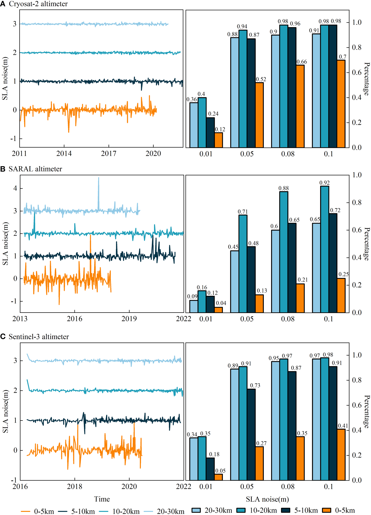
Noise level of SLA estimates of three altimeters in four different coastal distance bands. (A) Cryosat-2, (B) SARAL, (C) Sentinel-3.
We used the C3S SLA dataset to calculate R and RMSE (Figure 6) for verifying the feasibility of estimating water level of three altimeters and multi-altimeter in the coastal area of Beibu Gulf. This paper also utilized the Bland-Altman method to examine the consistency of altimeter-based water levels and C3S SLA data (Figure 7).
Figure 6

Comparison of the estimation accuracy between altimeter-based water levels and C3S data products. (A) Cryosat-2, (B) SARAL, (C) Sentinel-3, (D) Multi-altimeter.
Figure 7

The Bland–Altman plots present the agreement between altimeter-based water levels and C3S SLA products during 2011– 2021. (A) Cryosat-2, (B) SARAL, (C) Sentinel-3, (D) Multi-altimeter. Dashed, black line in the center of the plot presents mean value of the above described differences, and outer dashed yellow lines presents 95% level of agreement (mean − 1.96 standard deviation and mean + 1.96 standard deviation).
As can be seen from Figure 6, the altimeter-based water levels were in good agreement with the C3S SLA products (R>0.66), indicating that the application of the three altimeters to estimate the water level in the coastal zone of Beibu Gulf was more reliable. The multi-altimeter water level was consistent with the C3S products (R=0.669), indicating that it is feasible to combine the three altimeters to construct a long time series of water level, and the fused altimeter water level increased the spatial and temporal coverage of the observation data. The Bland-Altman plots in Figure 7 showed that the scattered points of the Cryosat-2, Sentinel-3, and multi-altimeter were all within the consistency limits, and >98% scattered points of the SARAL altimeter were within the consistency limits, demonstrating that the altimeter-based water levels and the C3S SLA products were in good agreement, further illustrated that it is feasible to apply the coastal zone water level estimating approach proposed in this paper to the water level estimating in the coastal Beibu Gulf. The RMSE of the altimeter-based water levels were all within 0.135m, reflecting that the accuracy of altimeter-based water levels estimated in this paper could reach the decimeter level, and three single altimeters have reached the centimeter level accuracy.
4.4 Analysis of water level dynamic changes
To clarify the water level dynamic change rule in the coastal area of Beibu Gulf, this paper combined two change detection algorithms, BFAST and MK, to detect the long-term change and abrupt change of water level in Beibu Gulf from 2011-2021. Figure 8 showed the MK test results for the time-series water levels from 2011-2021.
Figure 8

MK test results for time-series water levels from 2011-2021. (A) Cryosat-2, (B) SARAL, (C) Sentinel-3, (D) Multi-altimeter.
It can be seen from Figure 8 that there were multiple mutation points for the four time-series water levels, most of the UFk statistics were within the critical line of the significance level of 0.05, illustrating that the changes of the four time-series water levels were relatively smooth. In Figure 8A, Cryosat-2 time-series water level was in a decreasing trend from January 2011 to August 2011, and after August 2011, the water levels all showed an increasing trend, with 19.7% of the monthly average water levels exceeding the critical line of the significance level of 0.05, indicating a significant increase in water levels during this period. In Figure 8B, the SARAL time-series water level changed more frequently from 2013 to 2015, and the level followed an increasing trend after 2016, then raised from 2017 to 2019, and then decreased again in 2020 and 2021. In Figure 8C, the Sentinel-3 time-series water level was in a downward trend from July 2016 to May 2017, and the rest of the months were in an upward trend. In Figure 8D, there were 65% of the monthly average water level in the multi-altimeter displayed an increasing trend, with the monthly average water level from November 2020 to December 2021 being outside the threshold of significance level 0.05, indicating a significant increase in water levels during this period. In general, the four time-series water levels showed an overall increasing trend.
Table 7 counted the number of abrupt changes for the four time-series water levels in each season to better explain the abrupt changes. As can be seen from Table 7, Cryosat-2 and multi-altimeter water levels did not mutate in spring and winter, and the mutation points were concentrated in summer and autumn, proving that the water levels changed more slowly in winter and spring, and more drastically in summer and autumn. SARAL and Sentinel-3 water levels mutated in different seasons. SARAL water level had the most mutations in spring, and Sentinel-3 water level had the same number of mutations in each season. In addition, the four time-series water levels mutated in 2021, indicating that the water levels changed frequently in 2021.
Table 7
| Seasons | Cryosat-2 | SARAL | Sentinel-3 | Multi-altimeter |
|---|---|---|---|---|
| Spring | 0 | 9 | 2 | 0 |
| Summer | 1 | 2 | 2 | 3 |
| Autumn | 2 | 4 | 1 | 2 |
| Winter | 0 | 4 | 2 | 0 |
The mutation times of the time-series water levels in different seasons.
To further analyze the dynamic change characteristics of the coastal water level in the Beibu Gulf from 2011 to 2021, this study used the BFAST algorithm to further check the long-term change, seasonal change and abrupt change of the four time-series water levels (Figure 9).
Figure 9

Decomposition results of four time-series water levels based on the BFAST algorithm. (A) Cryosat-2, (B) SARAL, (C) Sentinel-3, (D) Multi-altimeter.
As shown in Figure 9, the seasonal component (St) of the four time-series water levels displayed a regular cyclical characteristic with a one-year variation period. On the trend component (Tt), the time-series water levels of the three single altimeters showed a monotonic upward trend, and the water level of the multi-altimeter increased monotonically from January 2011 to September 2012, with a breakpoint in September 2012 and a monotonic increase from October 2012 to December 2021. In the residual component (Rt), the four time-series water levels did not reveal a significant regularity. In addition, the original time series (Yt) of the four altimeter-based water levels displayed good consistency in intra-annual variation, showing an overall declining-rising-declining variation process, with a distinct peak and a minimum value throughout the year. The four time-series water levels varied slowly in January-March, and frequently in April-August. The lowest values occurred in May-August, after which the water levels presented an upward trend and reached a peak in October-November, with the monthly average water levels in September-December being significantly higher than those in January-August.
Based on mastering the historical change process of the coastal water level in Beibu Gulf from 2011 to 2021, this paper took the monthly average water level of multi-altimeter as the input data, utilized the LSTM model to simulate and predict the water level change trend in the coastal zone of Beibu Gulf from 2022 to 2031(Figure 10).
Figure 10

Predicted results of monthly average water level in the coastal zone of Beibu Gulf using the LSTM model. (A) true and predicted values for 2013-2021. (B) the error between predicted and true values for 2013-2021. (C) the future trend of monthly average water level from 2022-2031.
In Figure 10A, the monthly average water levels predicted by the LSTM model have good agreement with the true monthly average water levels, with R reaching 0.848 and RMSE of 0.049 m, indicating that it is feasible to predict the water level variation over a long time series using the LSTM algorithm. In Figure 10B, the standard deviation between the predicted water levels and the true water levels using the LSTM algorithm was small, and most of the standard deviation varied between 0.0005 and 0.08 m, which had good prediction accuracy. Therefore, we predicted the monthly average water level changes in the coastal zone of Beibu Gulf in the next 10 years (January 2022-December 2031), and the prediction results were displayed in Figure 10C. From Figure 10C, it can be found that the water level time series in Beibu Gulf in the next 10 years also had distinct seasonality, with a seasonal variation period of one year. In the interannual variation, the water level showed a slow upward trend from 2011-2021, with a water level rise rate of 8 mm/a, the water level change from 2022-2031 also displayed a slow upward trend, with a water level rise rate of about 0.6 mm/a.
5 Discussion
This paper found that the SEL algorithm achieved high accuracy classification of coastal waveforms with an average accuracy of 0.959 (Table 3). The SEL algorithm improved the average accuracy by 0.5%-1% over three single machine learning classification algorithms, proving that the SEL algorithm could effectively improve the classification accuracy of coastal waveforms, and this conclusion was consistent with the conclusion reached by Fu et al. (2022a). In addition, the SEL algorithm also displayed superior classification performance in recognizing coastal waveforms from different altimeters. In the Cryosat-2 altimeter, the SEL algorithm had the highest accuracy in recognizing ocean-like waveforms and complex waveforms. In the SARAL altimeter, the SEL algorithm had the highest accuracy in recognizing quasi-specular waveforms and complex waveforms. In the Sentinel-3 altimeter, the SEL algorithm had higher accuracy in recognizing all three coastal waveforms than the three single machine learning algorithms. The above findings demonstrated that the SEL algorithm was more adaptable to multi-source data and had good and stable performance in classifying coastal waveforms (Cai et al., 2020). Based on the coastal waveforms classification results of three altimeters using the SEL algorithm, this paper found that quasi-specular waveforms and complex waveforms within 0-5 km accounted for more than 60% of all waveforms (Table 4), and ocean-like waveforms within 5-30 km accounted for more than 80% of all waveforms. These results illustrated that the coastal waveforms within 0-5 km were heavily contaminated, and it is necessary to use multiple retrackers for optimal processing of different coastal waveforms.
Among the three retracking strategies proposed in this study, Threshold Retracker & ALES+ Retracker (TR_ALES+) exhibited the optimal retracking performance, followed by Threshold Retracker & Primary Peak COG Retracker (TR_PPCR), and finally Threshold Retracker & Primary Peak Threshold Retracker (TR_PPTR). Comparing the water level accuracy after retracking coastal waveforms with the three strategies (Table 5), it could be found that after retracking coastal waveforms using TR_ALES+, the R of SARAL altimeter improved by 0.089~0.133, RMSE decreased by 0.021~0.029m, and SD decreased by 0.009~0.010m, the R of Sentinel-3 altimeter improved by 0.411~0.475 and RMSE decreased by 0.008~0.015m. The above study also showed that the ALES+ retracker improved the coastal waveforms better than PPCR and PPTR retracker. However, there were differences in the improvement of coastal waveforms from different altimeters by ALES+ retracker. The water level accuracy after retracking coastal waveforms with multiple retrackers and single retracker (Table 6) identified that the overall retracking performance of the Sentinel-3 altimeter was better than the SARAL altimeter when only used ALES+ retracker. Due to the small study area of this paper and the small number of quasi-specular waveforms and complex waveforms, the water level accuracy after retracking coastal waveforms with multiple retrackers and single retracker did not show significant differences. In addition to the retracking method, the operation mode of the altimeter is also an important factor affecting the water level accuracy in coastal areas. The water level accuracy of the three altimeters (Figure 6) revealed that the water level accuracy of the Sentinel-3 altimeter in SAR mode was better than the SARAL altimeter in the LRM mode when the same TR_ALES+ retracker was used, with an R improvement of 0.078, indicating that the SAR altimeter outperformed the LRM altimeter in the coastal region, which was consistent with the findings of Fenoglio et al. (2021). Furthermore, the coastal water level estimating approach proposed in this paper did not obtain high-accuracy water level data, which may be due to the following reasons: on the one hand, the performance of altimeters in coastal areas decreased compared to the superior performance in the open ocean, as well demonstrated by Salameh et al. (2018). The results of Vignudelli et al. (2019) also showed that when the satellites were less than 6 km, the data availability decreased significantly. On the other hand, geophysical corrections such as dynamic atmospheric correction, wet tropospheric correction, and sea state bias may also lead to large uncertainties of satellite altimeters in coastal areas (Marti et al., 2021). The geophysical corrections used in this paper were all from three satellite altimeter, and more models can be considered in the future, such as the MOG2D model, GPD+ model, FES2014 model, and Composite SSB model (Peng and Deng, 2020).
In this study, the historical change processes of the four altimeter-based water levels were revealed using the BFAST and MK algorithms. The MK test results (Figure 8) for the four altimeter-based water levels illustrated that the MK algorithm could well characterize the abrupt changes and long-term change processes of the water level time series (Liang et al., 2018). The results based on the BFAST algorithm (Figure 9) for the four time-series water levels demonstrated that the BFAST algorithm could detect both long-term trends and abrupt changes in the water level time series, and also better describe the seasonal changes (Watts and Laffan, 2014). The change detection results of the four time-series water levels based on the BFAST and MK algorithms displayed that the water level in the coastal zone in Beibu Gulf presented a slow upward trend overall and had a one-year periodicity in seasonal changes, with the lowest water level occurring in May-August and the highest water level concentrated in October-November, similar to the experimental results of Sun et al. (2020). In addition, the 2021 China Sea Level Bulletin (Ministry of Natural Resources, 2022) reported that September-November was the seasonal high sea level period along the coast of Guangxi, which was consistent with the conclusion that the monthly average water levels in September-December were higher than the rest of the months reached in this paper. The LSTM model was used to predict the monthly average water level of the multi-altimeter from January 2011-December 2021 (Figure 10), and the correlation coefficient(R) between the predicted and true water level based on the LSTM model was 0.848, with an RMSE less than 0.05m, proving that the LSTM model could simulate the trend of the original water level time series well and had a strong prediction capability (Zhao et al., 2021). 2011-2031 water level displayed a slowly rising trend, and the rate of water level rise was 8 mm/a in 2011-2021 and about 0.6 mm/a in 2022-2031, and this conclusion was significantly different from that reported in the 2021 China Sea Level Bulletin (Ministry of Natural Resources, 2022). The main reason for this discrepancy was that only 11 years of water level time series were constructed in this paper, and the length of the time series was relatively short, which may not accurately reflect the historical water level change pattern in Beibu Gulf. In future studies, longer water level time series should be built, and algorithms such as Singular spectrum analysis (Shen et al., 2018), and Radial basis function (Yang et al., 2016) can be combined to further improve the accuracy of future trend prediction of coastal water level, to grasp more accurate water level dynamic change patterns and provide a scientific basis for the sustainable development of coastal areas.
6 Conclusion
This study presented a new method for estimating water levels of coastal zone in Beibu Gulf, south China, by combination of SEL-based waveform classifications and multiple retrackers using Cryosat-2, SARAL and Sentinel-3 altimeters from 2011-2021, and further tracked the dynamic change of water level using BFAST, MK and LSTM algorithms. This paper found that: (1) SEL algorithm effectively improved the classification accuracy of coastal waveforms, and produced better classification performance than single machine learning algorithms. Quasi-specular and complex echoes were the main coastal waveforms within 0-5 km, while ocean-like echo accounted for more than 80% of all waveforms beyond 5 km. (2) Combination of Threshold Retracker and ALES+ Retracker outperformed other two retracking strategies, and significantly improved the retrieval accuracy of water level in coastal areas. (3) Bland-Altman consistency test confirmed that altimeter-based measurements of coastal water level were consistent with the scientific dataset of C3S water level products at the 95% confidence interval, which indicated that the approach proposed in this study had a good performance on estimating coastal water levels, and monitoring its time-series dynamic changes using multi-sources altimeters. (4) We revealed that the coastal water level in Beibu Gulf exhibited a slow growth trend with an annual average growth rate of 8mm/a in 2011-2021, and the intra-year water level presented a fluctuation change with the declining-rising-declining procedures. We also found that the lowest average water level concentrated in May-August and the highest average water level focused on October-November. These results can provide guidance for scientific monitoring and sustainable management of coastal zones.
Statements
Data availability statement
Publicly available datasets were analyzed in this study. This data can be found here: https://climate.copernicus.eu/.
Author contributions
JQ wrote the manuscript, and researched model, collected, and analyzed the data. BF planned the study, analyzed the data, and wrote the manuscript. HH, FW, LL and DF directed work and supervision. SL, HY, XH, and YL collected, and analyzed the data. JQ and BF did the main manuscript revision and editing. All authors contributed to the article and approved the submitted version.
Funding
This work was supported by the Guangxi Science & Technology Program (Grant number GuikeAD20159037), the Innovation Project of Guangxi Graduate Education (Grant number YCSW2022328), the National Natural Science Foundation of China (Grant number 41801071 and 42064002), the Natural Science Foundation of Guangxi Province (CN) (Grant number 2018GXNSFBA281015), and the ‘Ba Gui Scholars’ program of the provincial government of Guangxi, the Guilin University of Technology Foundation (Grant number GUTQDJJ2017096).
Acknowledgments
We appreciate the reviewers for their comments and suggestions, which helped to improve the quality of this manuscript. We would like to thank the ESA for providing Cryosat-2 data, the AVISO+ for providing SARAL data, the EUMETSAT for providing Sentinel-3 data, and the Copernicus Climate Change Service for providing daily SLA dataset. We also appreciate Marcello Passaro professor for providing help about ALES+ method
Conflict of interest
The authors declare that the research was conducted in the absence of any commercial or financial relationships that could be construed as a potential conflict of interest.
Publisher’s note
All claims expressed in this article are solely those of the authors and do not necessarily represent those of their affiliated organizations, or those of the publisher, the editors and the reviewers. Any product that may be evaluated in this article, or claim that may be made by its manufacturer, is not guaranteed or endorsed by the publisher.
References
1
Adebisi N. Balogun A.-L. Min T. H. Tella A. (2021). Advances in estimating Sea level rise: A review of tide gauge, satellite altimetry and spatial data science approaches. Ocean Coast. Manage.208, 105632. doi: 10.1016/j.ocecoaman.2021.105632
2
Alashan S. (2020). Combination of modified Mann-Kendall method and Şen innovative trend analysis. Eng. Rep.2, e12131. doi: 10.1002/eng2.12131
3
Arabsahebi R. Voosoghi B. Tourian M. J. (2020). A denoising–classification–retracking method to improve spaceborne estimates of the water level–surface–volume relation over the urmia lake in Iran. Int. J. Remote Sens.41, 506–533. doi: 10.1080/01431161.2019.1643938
4
Arns A. Dangendorf S. Jensen J. Talke S. Bender J. Pattiaratchi C. (2017). Sea-Level rise induced amplification of coastal protection design heights. Sci. Rep.7, 1–9. doi: 10.1038/srep40171
5
Birgiel E. Ellmann A. Delpeche-Ellmann N. (2018). Examining the performance of the sentinel-3 coastal altimetry in the Baltic Sea using a regional high-resolution geoid model. 2018 Baltic Geodetic Congress (BGC Geomatics) IEEE, 196–201. doi: 10.1109/BGC-Geomatics.2018.00043
6
Bukhari A. H. Raja M. A. Z. Sulaiman M. Islam S. Shoaib M. Kumam P. (2020). Fractional neuro-sequential ARFIMA-LSTM for financial market forecasting. IEEE Access8, 71326–71338. doi: 10.1109/ACCESS.2020.2985763
7
Cai Y. Li X. Zhang M. Lin H. (2020). Mapping wetland using the object-based stacked generalization method based on multi-temporal optical and SAR data. Int. J. Appl. Earth Observation Geoinfo.92, 102164. doi: 10.1016/j.jag.2020.102164
8
Cazenave A. Palanisamy H. Ablain M. (2018). Contemporary sea level changes from satellite altimetry: What have we learned? what are the new challenges? Adv. Space Res.62, 1639–1653. doi: 10.1016/j.asr.2018.07.017
9
Chen J. Liao J. (2020). Monitoring lake level changes in China using multi-altimeter data, (2016–2019). J. Hydrol.590, 125544. doi: 10.1016/j.jhydrol.2020.125544
10
Davis C. H. (1997). A robust threshold retracking algorithm for measuring ice-sheet surface elevation change from satellite radar altimeters. IEEE Trans. Geosci. Remote Sens.35, 974–979. doi: 10.1109/36.602540
11
Faugère Y. Taburet G. Ballarotta M. Pujol I. Legeais J. F. Maillard G. et al . (2022). DUACS DT2021: 28 years of reprocessed sea level altimetry products. EGU Gen. Assembly Conf. Abstracts, EGU22–E7479. doi: 10.5194/egusphere-egu22-7479
12
Fenoglio L. Dinardo S. Uebbing B. Buchhaupt C. Gärtner M. Staneva J. et al . (2021). Advances in NE-Atlantic coastal sea level change monitoring by delay Doppler altimetry. Adv. Space Res.68, 571–592. doi: 10.1016/j.asr.2020.10.041
13
Fu B. He X. Yao H. Liang Y. Deng T. He H. et al . (2022a). Comparison of RFE-DL and stacking ensemble learning algorithms for classifying mangrove species on UAV multispectral images. Int. J. Appl. Earth Observation Geoinfo.112, 102890. doi: 10.1016/j.jag.2022.102890
14
Fu B. Sun J. Wang Y. Yang W. He H. Liu L. et al . (2022b). Evaluation of LAI estimation of mangrove communities using DLR and ELR algorithms with UAV, hyperspectral, and SAR images. Front. Mar. Sci.9, 944454. doi: 10.3389/fmars.2022.944454
15
Güçlü Y. S. (2020). Improved visualization for trend analysis by comparing with classical Mann-Kendall test and ITA. J. Hydrol.584, 124674. doi: 10.1016/j.jhydrol.2020.124674
16
Jain M. Andersen O. B. Dall J. Stenseng L. (2015). Sea Surface height determination in the Arctic using cryosat-2 SAR data from primary peak empirical retrackers. Adv. Space Res.55, 40–50. doi: 10.1016/j.asr.2014.09.006
17
Jiang C. Lin M. Wei H. (2019). A study of the technology used to distinguish Sea ice and seawater on the haiyang-2A/B (HY-2A/B) altimeter data. Remote Sens.11, 1490. doi: 10.3390/rs11121490
18
Jia M. Wang Z. Zhang Y. Ren C. Song K. (2015). Landsat-based estimation of mangrove forest loss and restoration in guangxi province, China, influenced by human and natural factors. IEEE J. Selected Topics Appl. Earth Observations Remote Sens.8, 311–323. doi: 10.1109/JSTARS.2014.2333527
19
Kang D. Lv Y. Chen Y.y. (2017). Short-term traffic flow prediction with LSTM recurrent neural network. 2017 IEEE 20th Int. Conf. Intelligent Transportation Syst. (ITSC), 1–6. doi: 10.1109/ITSC.2017.8317872
20
Kisi O. Ay M. (2014). Comparison of Mann–Kendall and innovative trend method for water quality parameters of the kizilirmak river, Turkey. J. Hydrol.513, 362–375. doi: 10.1016/j.jhydrol.2014.03.005
21
Liang S. Wang W. Zhang D. (2018). Characteristics of annual and seasonal precipitation variation in the upstream of minjiang river, southwestern China. Adv. Meteorol.2018, 1362708. doi: 10.1155/2018/1362708
22
Marti F. Cazenave A. Birol F. Passaro M. Léger F. Niño F. et al . (2021). Altimetry-based sea level trends along the coasts of Western Africa. Adv. Space Res.68, 504–522. doi: 10.1016/j.asr.2019.05.033
23
Melet A. Teatini P. Le Cozannet G. Jamet C. Conversi A. Benveniste J. et al . (2020). Earth observations for monitoring marine coastal hazards and their drivers. Surveys Geophys.41, 1489–1534. doi: 10.1007/s10712-020-09594-5
24
Mendes M. P. Rodriguez-Galiano V. Aragones D. (2022). Evaluating the BFAST method to detect and characterise changing trends in water time series: A case study on the impact of droughts on the Mediterranean climate. Sci. Total Environ.846, 157428. doi: 10.1016/j.scitotenv.2022.157428
25
Ministry of Natural Resources (2022). 2021 bulletin of China Sea level. Available at: http://gi.mnr.gov.cn/202205/t20220507_2735509.html
26
Orejarena-Rondón A. F. Sayol J. M. Marcos M. Otero L. Restrepo J. C. Hernández-Carrasco I. et al . (2019). Coastal impacts driven by sea-level rise in cartagena de indias. Front. Mar. Sci.6. doi: 10.3389/fmars.2019.00614
27
Palanisamy H. Cazenave A. Henry O. Prandi P. Meyssignac B. (2015). Sea-Level variations measured by the new altimetry mission SARAL/AltiKa and its validation based on spatial patterns and temporal curves using Jason-2, tide gauge data and an overview of the annual Sea level budget. Mar. Geodesy38, 339–353. doi: 10.1080/01490419.2014.1000469
28
Passaro M. Rose S. K. Andersen O. B. Boergens E. Calafat F. M. Dettmering D. et al . (2018). ALES+: Adapting a homogenous ocean retracker for satellite altimetry to sea ice leads, coastal and inland waters. Remote Sens. Environ.211, 456–471. doi: 10.1016/j.rse.2018.02.074
29
Peacock N. R. Laxon S. W. (2004). Sea Surface height determination in the Arctic ocean from ERS altimetry. J. Geophys. Res.: Oceans109, C07001. doi: 10.1029/2001JC001026
30
Peng F. Deng X. (2020). Improving precision of high-rate altimeter sea level anomalies by removing the sea state bias and intra-1-Hz covariant error. Remote Sens. Environ.251, 112081. doi: 10.1016/j.rse.2020.112081
31
Peng F. Deng X. Cheng X. (2021). Quantifying the precision of retracked Jason-2 sea level data in the 0–5 km Australian coastal zone. Remote Sens. Environ.263, 112539. doi: 10.1016/j.rse.2021.112539
32
Poisson J.-C. Quartly G. D. Kurekin A. A. Thibaut P. Hoang D. Nencioli F. (2018). Development of an ENVISAT altimetry processor providing sea level continuity between open ocean and Arctic leads. IEEE Trans. Geosci. Remote Sens.56, 5299–5319. doi: 10.1109/TGRS.2018.2813061
33
Prandi P. Poisson J.-C. Faugère Y. Guillot A. Dibarboure G. (2021). Arctic Sea surface height maps from multi-altimeter combination. Earth System Sci. Data13, 5469–5482. doi: 10.5194/essd-13-5469-2021
34
Rahman M. Chen N. Elbeltagi A. Islam M. M. Alam M. Pourghasemi H. R. et al . (2021). Application of stacking hybrid machine learning algorithms in delineating multi-type flooding in Bangladesh. J. Environ. Manage.295, 113086. doi: 10.1016/j.jenvman.2021.113086
35
Raynal M. Labroue S. Moreau T. Boy F. Picot N. (2018). From conventional to delay Doppler altimetry: A demonstration of continuity and improvements with the cryosat-2 mission. Adv. Space Res.62, 1564–1575. doi: 10.1016/j.asr.2018.01.006
36
Reimann L. Vafeidis A. T. Brown S. Hinkel J. Tol R. S. J. (2018). Mediterranean UNESCO World heritage at risk from coastal flooding and erosion due to sea-level rise. Nat. Commun.9, 4161. doi: 10.1038/s41467-018-06645-9
37
Salameh E. Frappart F. Marieu V. Spodar A. Parisot J. P. Hanquiez V. et al . (2018). Monitoring Sea level and topography of coastal lagoons using satellite radar altimetry: The example of the arcachon bay in the bay of Biscay. Remote Sens.10, 297. doi: 10.3390/rs10020297
38
Shen Y. Guo J. Liu X. Kong Q. Guo L. Li W. (2018). Long-term prediction of polar motion using a combined SSA and ARMA model. J. Geodesy92, 333–343. doi: 10.1007/s00190-017-1065-3
39
Shi X. Chen Z. Wang H. Yeung D.-Y. Wong W.-K. Woo W.-c. (2015). Convolutional LSTM network: A machine learning approach for precipitation nowcasting. arXiv preprint arXiv.1506.04214. doi: 10.48550/arXiv.1506.04214
40
Shu S. Liu H. Beck R. A. Frappart F. Korhonen J. Xu M. et al . (2020). Analysis of sentinel-3 SAR altimetry waveform retracking algorithms for deriving temporally consistent water levels over ice-covered lakes. Remote Sens. Environ.239, 111643. doi: 10.1016/j.rse.2020.111643
41
Sonobe R. Yamaya Y. Tani H. Wang X. Kobayashi N. Mochizuki K.-i. (2018). Crop classification from sentinel-2-derived vegetation indices using ensemble learning. J. Appl. Remote Sens.12, 26019. doi: 10.1117/1.JRS.12.026019
42
Sun Q. Wan J. Liu S. (2020). Estimation of Sea level variability in the China Sea and its vicinity using the SARIMA and LSTM models. IEEE J. Selected Topics Appl. Earth Observations Remote Sens.13, 3317–3326. doi: 10.1109/JSTARS.2020.2997817
43
Taburet G. Sanchez-Roman A. Ballarotta M. Pujol M.-I. Legeais J.-F. Fournier F. et al . (2019). DUACS DT2018: 25 years of reprocessed sea level altimetry products. Ocean Sci.15, 1207–1224. doi: 10.5194/os-15-1207-2019
44
Taherkhani M. Vitousek S. Barnard P. L. Frazer N. Anderson T. R. Fletcher C. H. (2020). Sea-Level rise exponentially increases coastal flood frequency. Sci. Rep.10, 6466. doi: 10.1038/s41598-020-62188-4
45
Tran N. Vandemark D. Zaron E. D. Thibaut P. Dibarboure G. Picot N. (2021). Assessing the effects of sea-state related errors on the precision of high-rate Jason-3 altimeter sea level data. Adv. Space Res.68, 963–977. doi: 10.1016/j.asr.2019.11.034
46
Verron J. Sengenes P. Lambin J. Noubel J. Steunou N. Guillot A. et al . (2015). The SARAL/AltiKa altimetry satellite mission. Mar. Geodesy38, 2–21. doi: 10.1080/01490419.2014.1000471
47
Vignudelli S. Birol F. Benveniste J. Fu L.-L. Picot N. Raynal M. et al . (2019). Satellite altimetry measurements of Sea level in the coastal zone. Surveys Geophys.40, 1319–1349. doi: 10.1007/s10712-019-09569-1
48
Villadsen H. Deng X. Andersen O. B. Stenseng L. Nielsen K. Knudsen P. (2016). Improved inland water levels from SAR altimetry using novel empirical and physical retrackers. J. Hydrol.537, 234–247. doi: 10.1016/j.jhydrol.2016.03.051
49
Watts L. M. Laffan S. W. (2014). Effectiveness of the BFAST algorithm for detecting vegetation response patterns in a semi-arid region. Remote Sens. Environ.154, 234–245. doi: 10.1016/j.rse.2014.08.023
50
Xu Y. Yu L. Peng D. Zhao J. Cheng Y. Liu X. et al . (2020). Annual 30-m land use/land cover maps of China for 1980–2015 from the integration of AVHRR, MODIS and landsat data using the BFAST algorithm. Sci. China Earth Sci.63, 1390–1407. doi: 10.1007/s11430-019-9606-4
51
Yang R. Er P. V. Wang Z. Tan K. K. (2016). An RBF neural network approach towards precision motion system with selective sensor fusion. Neurocomputing199, 31–39. doi: 10.1016/j.neucom.2016.01.093
52
Zhao J. Cai R. Sun W. (2021). Regional sea level changes prediction integrated with singular spectrum analysis and long-short-term memory network. Adv. Space Res.68, 4534–4543. doi: 10.1016/j.asr.2021.08.017
53
Zygmuntowska M. Khvorostovsky K. Helm V. Sandven S. (2013). Waveform classification of airborne synthetic aperture radar altimeter over Arctic sea ice. Cryos.7, 1315–1324. doi: 10.5194/tc-7-1315-2013
Summary
Keywords
coastal zone, multi-altimeter, ensemble learning, ALES+ retracker, BFAST and LSTM, water level change monitoring
Citation
Qin J, Li S, Yao H, Fu B, He H, Wang F, Liu L, Fan D, He X and Li Y (2023) Synergistic multi-altimeter for estimating water level in the coastal zone of Beibu Gulf using SEL, ALES + and BFAST algorithms. Front. Mar. Sci. 9:1113387. doi: 10.3389/fmars.2022.1113387
Received
01 December 2022
Accepted
14 December 2022
Published
10 January 2023
Volume
9 - 2022
Edited by
Mingming Jia, Northeast Institute of Geography and Agroecology (CAS), China
Reviewed by
Chao Chen, Zhejiang Ocean University, China; Qing Xia, Changsha University of Science and Technology, China
Updates
Copyright
© 2023 Qin, Li, Yao, Fu, He, Wang, Liu, Fan, He and Li.
This is an open-access article distributed under the terms of the Creative Commons Attribution License (CC BY). The use, distribution or reproduction in other forums is permitted, provided the original author(s) and the copyright owner(s) are credited and that the original publication in this journal is cited, in accordance with accepted academic practice. No use, distribution or reproduction is permitted which does not comply with these terms.
*Correspondence: Bolin Fu, fubolin@glut.edu.cn; Lilong Liu, lllong99@glut.edu.cn
This article was submitted to Marine Conservation and Sustainability, a section of the journal Frontiers in Marine Science
Disclaimer
All claims expressed in this article are solely those of the authors and do not necessarily represent those of their affiliated organizations, or those of the publisher, the editors and the reviewers. Any product that may be evaluated in this article or claim that may be made by its manufacturer is not guaranteed or endorsed by the publisher.