Long-Term and Seasonal Variability of Wind and Wave Extremes in the Arctic Ocean

1 Introduction

Arctic sea ice extent has been declining sharply at a rate of 13% per decade and with thickness reducing about 66% over the past 60 years (see IPCC, 2019). Variations of the sea ice cover have been the cause of notable changes to meteorological and oceanographic conditions in the Arctic Ocean (e.g. Thomson and Rogers, 2014; Liu et al., 2016; Stopa et al., 2016; Thomson et al., 2016; Waseda et al., 2018; Casas-Prat and Wang, 2020). Emerging open waters—see the minimum sea ice extent in September 1991 and September 2018 in Figure 1 —provide longer fetches for surface waves to build up more energy and increase in magnitude (Thomson and Rogers, 2014; Thomson et al., 2016). Concurrently, an increase of wave height impacts profoundly on the already weak sea ice cover by enhancing breakup and melting processes in a feedback mechanism (Thomson et al., 2016; Dolatshah et al., 2018; Passerotti et al., 2022). In addition, coastlines and coastal communities have been impacted by intensifying erosion with coastline retreat rates up to 25 m per year (e.g. Jones et al., 2009; Gunther et al., 2015).

FIGURE 1

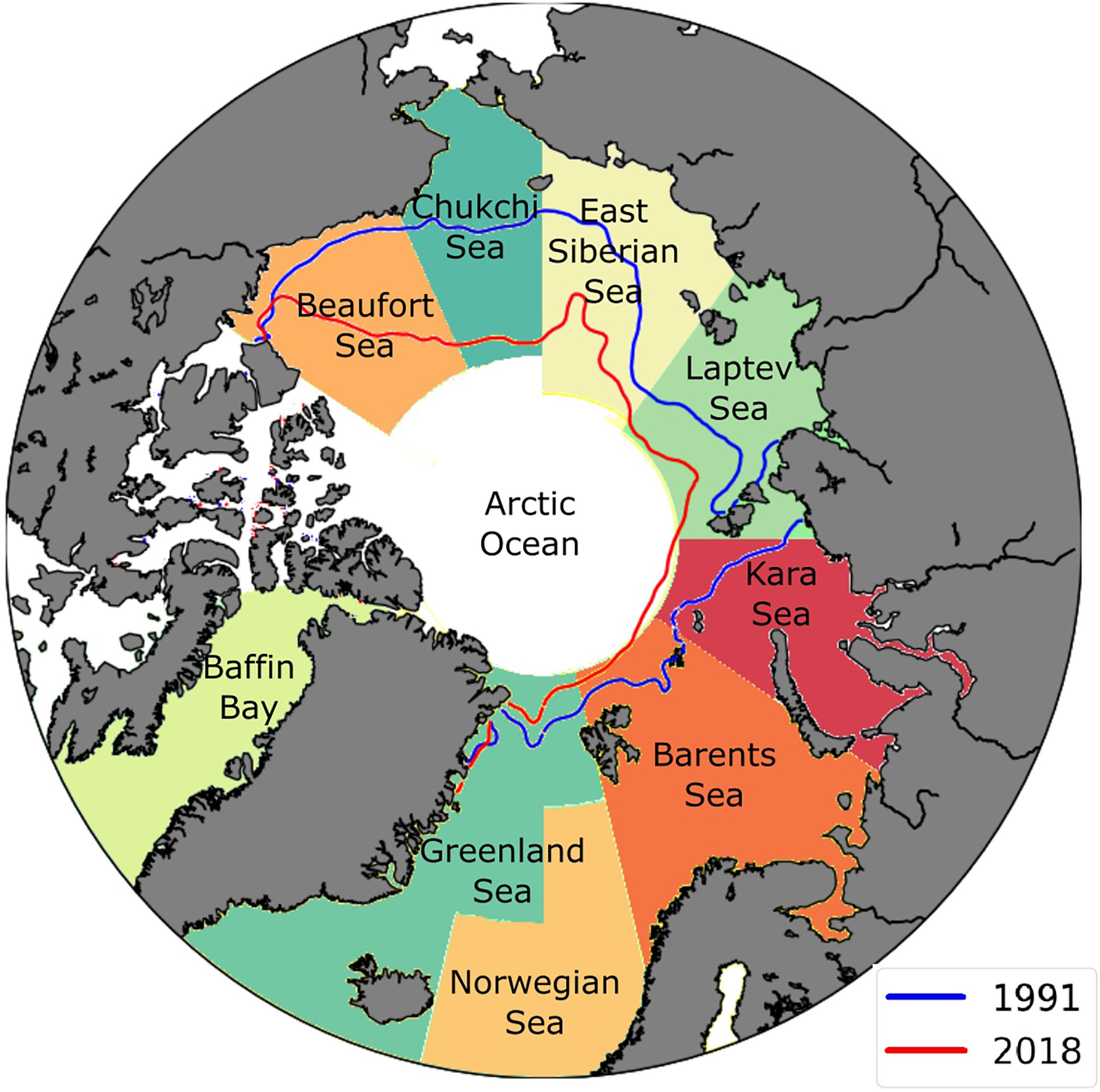
Figure 1 Regions of the Arctic Ocean used in this study with lines showing sea ice extent in September of 1991 (blue) and 2018 (red). Sea ice concentration dataset from ERA5 reanalysis.

Ocean climate evaluated from satellite observations (Liu et al., 2016) for the months of August and September—the period of minimum ice coverage—reveals weak or even negative trends of average offshore wind speeds over the period between 1996 and 2015, while notable upward trends were detected in the higher 90^th and 99^th percentiles across the entire Arctic Ocean, except for the Greenland sea. Unlike winds, waves showed more substantial increasing rates even for average values, especially in the Chukchi, Laptev, Kara seas and Baffin Bay.

Satellite observations have temporal and spatial limitations, which are exacerbated in the Arctic where most of the altimeter sensors do not usually cover latitudes higher than 82°. Numerical models, on the contrary, provide more consistent data sets for climate analysis in this region. Stopa et al. (2016) estimated trends using a 23-year model hindcast and found that simulated average wind speed exhibits a weak increasing trend, especially in the Pacific sector of the Arctic Ocean, slightly differing from the satellite-based observations in Liu et al. (2016). Average wave heights, however, were found to be consistent with altimeter data. Waseda et al. (2018) used the ERA-Interim reanalysis database (Dee et al., 2011) to evaluate the area-maximum wind speed and wave height in the months of August, September and October from the period 1979-2016 in the Beaufort, Chukchi, East Siberian and Laptev seas. Their analysis indicated robust increasing trends for both variables, with most significant changes in October: ≈0.06ms^-1 per year for wind speed and ≈2cm per year for mean significant wave height. Recently, Casas-Prat and Wang (2020) simulated historical (1979-2005) and future (2081-2100) sea state conditions to evaluate changes in regional annual maximum significant wave height, under high baseline emission scenarios (RCP8.5). Their results indicated that wave height is projected to increase at a rate of approximately 3 cm per year, which is more than 0.5% per year in terms of annual maxima.

Previous assessments of ocean climate in the Arctic have focused on annual or monthly values and often paid specific attention to summer months. A comprehensive evaluation of climate and related changes cannot, however, ignore extremes. Classically, extreme metocean conditions are estimated with an extreme value analysis (EVA), where observations are fitted to a theoretical probability distribution to extrapolate values at low probability levels, such as those occurring on average once every 100 years (normally referred to as the 100-year return period event, see Ochi, 2005; Bitner-Gregersen and Toffoli, 2014; Thomson and Emery, 2014; Clancy et al., 2016; Meucci et al., 2020, for examples of applications in different fields of ocean engineering, physical oceanography and climate). Therefore, the EVA has to rely on long records spanning over one or more decades (observations typically cover more than a 1/3 of the return period), to be statistically significant. Motivated by the need of very long time series, the EVA requires the fundamental assumption that the statistical properties of a specific variable do not change over time, namely the process is stationary. For the strongly seasonal and rapidly changing Arctic environment, however, the hypothesis of stationarity cannot hold for an extended period of time. The inevitable time-dependency of the statistical distribution of a certain environmental stochastic process translates into a time-dependency of the parameters of the associated extreme value distribution (see more details in e.g. Renard et al., 2013; De Leo et al., 2021), invalidating the fundamental assumption of the EVA.

An alternative approach that better fits the highly dynamic nature of the Arctic is the estimation of time-varying extreme values with a non-stationary analysis (see, for example, Coles et al., 2001; Mendez et al., 2006; Galiatsatou and Prinos, 2011; Cheng et al., 2014; Mentaschi et al., 2016; De Leo et al., 2021, for a general overview). There are a number of methods for the estimation of time-varying extreme value distributions from non-stationary time series. A functional approach is the transformed-stationary extreme value analysis (TS-EVA) proposed by Mentaschi et al. (2016). The method consists of transforming a non-stationary time series with a normalisation based on the time-varying mean and standard deviation into a stationary counterpart, for which the classical EVA theory can be applied. Subsequently, an inverse transformation allows the conversion of the EVA results to time-varying extreme values.

Here we apply the TS-EVA method to assess time-varying extremes in the Arctic Ocean. The assessment is performed on a data set consisting of a long-term hindcast—from January 1991 to December 2018—that was obtained using the WAVEWATCH III (WW3, Tolman, 2009) spectral wave model forced with ERA5 reanalysis wind speeds (Hersbach et al., 2019). A description of the model and its validation is reported in Section 2.1. Model data are processed with the TS-EVA to determine extreme values for wind forcing and wave height. Long-term trends are investigated with a nonseasonal approach; seasonal variability is considered with a concurrent seasonal method (Section 2.2). Results are discussed in terms of regional distributions and areal averages in Sections 3 and 4. Concluding remarks are presented in the last Section.

2 Method

2.1 Wave Hindcast

A 28-year (from 1991 to 2018) wave hindcast of the Arctic Ocean (Cabral et al., 2021) was carried out with the WAVEWATCH III (WW3) spectral wave model—version 6.07—to build a database of sea state conditions, which is consistent in space and time. A regional model domain covering the area above latitude 53.17°N was set up in an Arctic Polar Stereographic Projection with a horizontal resolution varying from 9 to 22 km (this configuration was found to optimise the accuracy of model results in relation to recorded data and computational time). The bathymetry was extracted from the ETOPO1 database (Amante and Eakins, 2009). The regional set up was then forced with ERA5 atmospheric data and sea ice coverage (Hersbach et al., 2019). The model physics were defined by the observation-based ST6 source term package (Liu et al., 2019), which accounts for wind-wave interaction and white capping dissipation processes, and the discrete interaction approximation (DIA, see Komen et al., 1984), which describes nonlinear interactions. The model was run without wave-ice interaction modules as the focus is on the open ocean and not the marginal ice zone; regions of sea ice with concentration larger than 25% were therefore treated as land. Note that higher thresholds of sea ice concentration are not ideal as they would produce significant wave attenuation (see for example Kohout et al., 2020; Alberello et al., 2021), requiring specific waves-in-ice physics. Boundary conditions were imposed on the regional model to account for energetic swells coming from the North Atlantic. To this end, boundaries were forced by incoming sea states from WW3 global runs with 1-degree spatial resolution (see Zieger et al., 2015, for general details of the set up). The global model used ERA5 wind forcing and the ST6 source term package. Simulations were run with a spectral domain of 32 frequency and 24 directional bins (directional resolution of 15 degrees). The minimum frequency was set at 0.0373 Hz and the frequency increment factor was set at 1.1, providing a frequency range of 0.0373-0.715 Hz. Grid outputs were stored every 3 hours.

Calibration of the ST6 source terms only requires adjustments of the wind-wave growth parameter (CDFAC, see e.g. Fernandez et al., 2021, for a discussion on model sensitivity to this parameter). This was performed by testing the model outputs (significant wave height) against altimeter data across six different satellite missions (ERS1, ERS2, ENVISAT, GFO, CRYOSAT-2 and Altika SARAL, see Queffeulou and Croize-Fillon, 2015) and for the period August-September 2014. The best agreement for the regional set up was achieved for CDFAC = 1.23 with correlation coefficient R=0.95, scatter index SI ≈ 1% and root mean square error RMSE ≈ 0.3mm (see e.g. Thomson and Emery, 2014, for details on error metrics). The configuration was further validated by comparing all modelled significant wave height values against matching altimeter observations for an independent period of four years from 2012 to 2016. Figure 2A shows the regional model outputs versus collocated altimeter data for the validation runs. Generally, the model correlates well with observations: R = 0.97, SI = 16%, and RMSE = 0.38m. The residuals between model and altimeters as a function of the observations are reported in Figure 2B for data in the 90^th percentile. The comparison indicates a satisfactory level of agreement for the upper range of wave heights (H_s > 4m): R = 0.86, SI = 11%, and RMSE = 0.63m. Model outputs are also consistent with ERA5 reanalysis, with a R = 0.99, RMSE = 0.27m and NBIAS of 2.3% for all data (Figure 2C), and R = 0.95, RMSE = 0.52m and NBIAS of 1.4% for the upper percentiles (Figure 2D). Note, however, that the WW3 model hindcast used herein predicts slightly higher wave heights and is marginally more accurate in replicating satellite observations than ERA5 (see assessment of ERA5 performance in Law-Chune et al., 2021) due to enhanced spatial and temporal resolution, making it more suitable for the present analysis.

FIGURE 2

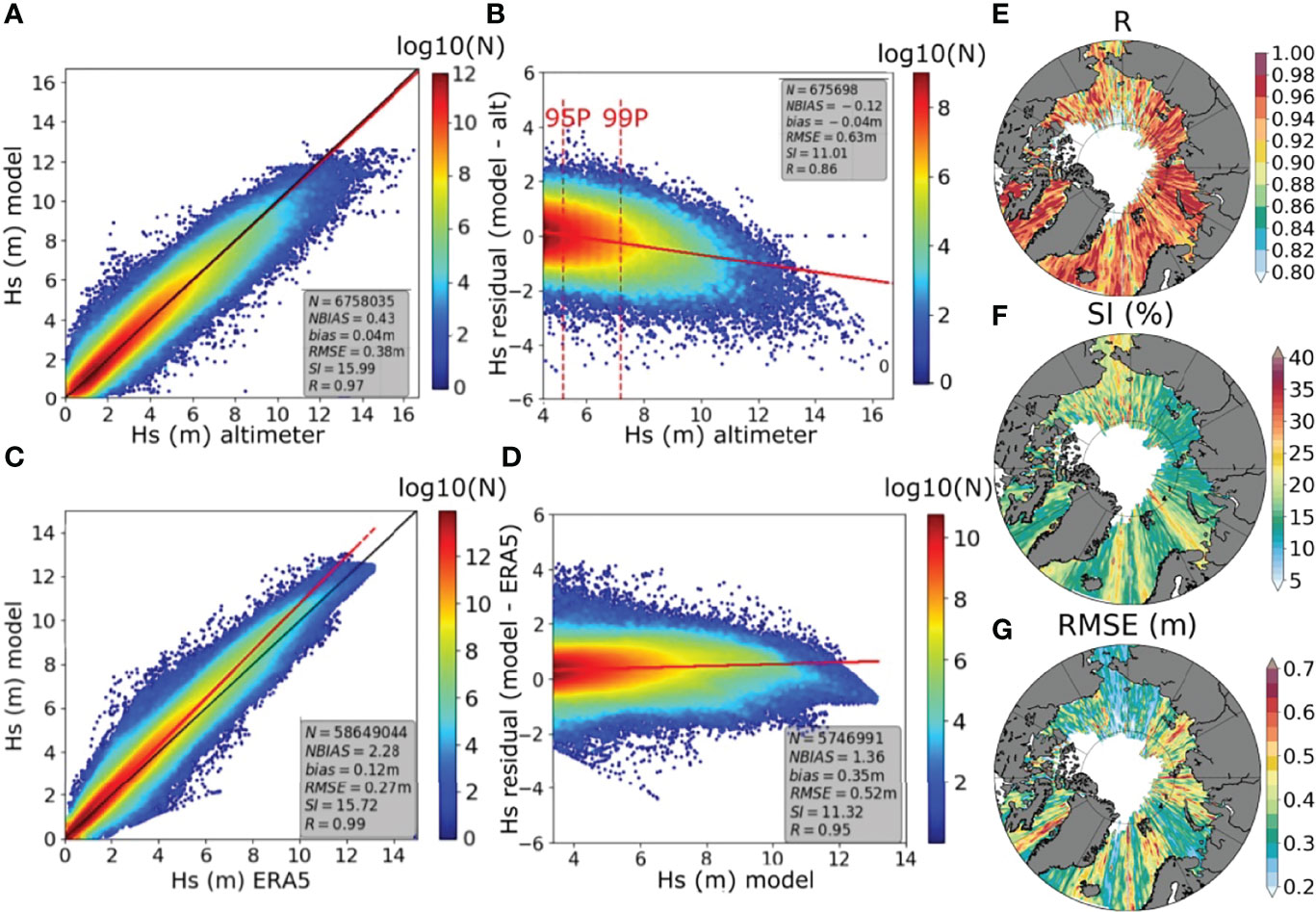
Figure 2 Validation of significant wave height for the period 2012–2016 with ST6 core physics. Comparison against altimeter observations: (A) all data and (B) 90th percentile. Comparison against ERA reanalysis: (C) all data and (D) 90th percentile and above. The black line represents the 1:1 agreement and the red lines are the linear regression. Regional distribution of error metrics (in relation to altimeter observations and data in the 90th percentile): (E) correlation, (F) scatter index, and (G) root mean square error.

The regional distribution of model errors (with respect to altimeter observations and for data in the 90^th percentile) is reported in Figures 2E–G. The model performed well across the entire Arctic Ocean with no specific regions affected by significant errors, noting that the analysis is limited to deep water regions where altimeter data is not contaminated by land.

The validation above considers matches of collocated values in time and space. An extreme value analysis applied to model results would require a further validation of e.g. 100-year return period significant wave height against in-situ or remotely sensed observations. Long duration (more than 20-years) in-situ buoy records are not available in the Arctic. Although altimeter data can be used for long term statistical analysis (Vinoth and Young, 2011; Takbash et al., 2019), low observation density and contamination of land and sea ice in the satellite footprints result in significant under-sampling and thus uncertainties of extreme value estimates (Takbash and Young, 2019). Thereby, the lack of reliable independent long term observations hampers a thorough verification of an extreme value analysis.

2.2 Transformed Stationary Extreme Value Analysis

The TS-EVA method developed by Mentaschi et al. (2016) is applied herein without any modifications, to extract time-varying information on climate extremes. In this section, we only provide a brief summary of the approach, while a more detailed discussioncan be found in Mentaschi et al. (2016); De Leo et al. (2021).

The method is based on three main steps. In the first step, the original non-stationary time series (see an example of significant wave height for the Kara sea in Figure 3A, where an initial downward trend between 1993 and 1999 is followed by a clear positive trend) is transformed into a stationary counterpart that can be processed using classical EVA methods. The transformation is based on the following equation:

$\begin{array}{ll}x\left(t\right)=\frac{y\left(t\right)-T_y\left(t\right)}{S_y\left(t\right)}& (1)\end{array}$

where y(t) is the non-stationary time-series, x(t) is the stationary counterpart, T_y(t) is the trend of y(t) and the S_y(t) is its standard deviation. Computation of T_y(t) and S_y(t) relies on algorithms based on running means and running statistics. This approach acts as a low-pass filter, which removes the variability within a specified time window W (hereafter this approach is referred to as nonseasonal). The time window has to be short enough to incorporate the desired variability, but long enough to eliminate noise and short-term variability; the optimal length for W was found to be 5 years due to the rapid sea ice melting occurring in the last few decades. The transformation results in time series with zero trend, zero mean and a standard deviation of one. In order to further verify stationarity, Mentaschi et al. (2016) also recommend that the skewness and kurtosis are approximately constant as a function of time. In the present application, representative transformed time series for each of the major Artic Ocean basins (Figure 1) were examined and their skewness and kurtosis evaluated. In all cases these values varied by less than 15% over the full duration of the model data set, in agreement with test results reported by Mentaschi et al. (2016). Thereby, we concluded that the transformed time series are approximately stationary.

FIGURE 3

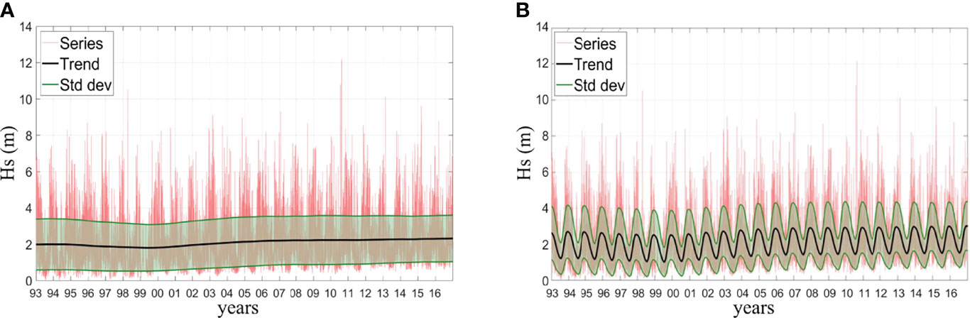
Figure 3 TS-EVA of the projections of significant wave height for a point located in the Kara Sea. The time series of Hs (m), its long-term trend and standard deviation computed with a time window of 5 years obtained with (A) the nonseasonal approach and (B) with the seasonal approach.

In the second step, the stationary time-series x(t) is processed with a standard EVA approach. Herein, a peaks-over-threshold method (POT, see e.g. Thomson and Emery, 2014, for a general overview) was applied to extract extreme values from the records with a threshold set at the 90^th percentile. A Generalised Pareto Distribution (GPD, e.g. Thomson and Emery, 2014).

$\begin{array}{ll}F\left(x\right)=1-\left[1+k{\left(\frac{x-A}{B}\right)}^{\frac{-1}{k}}\right]& (2)\end{array}$

where A is the threshold and B and k are the scale and shape parameters respectively, was fitted to the data in order to derive an extreme value distribution; a Kolmogorov Smirnov test (see e.g. Chu et al., 2019) was applied to validate the fit. Note that the parameters A and B are time-dependent and change with trends, standard deviation, and seasonality in the TS-EVA approach. To ensure statistical independence, peaks were selected at least 48 hours apart. Furthermore, to ensure a stable probability distribution, a minimum of 1000 peaks was selected for each grid point of the model domain (Meucci et al., 2018), meaning that regions free of sea ice less than about two months per year were excluded from the analysis.

It should be noted that the selection of the threshold affects the estimate of extreme values. The threshold has to be neither too high, in order to include sufficient data points and hence ensure a stable fit of equation 2, nor too low, so that non-extreme values are excluded from the analysis. For significant wave height, the threshold is normally a percentile value from 90^th, as in this study, to 95^th percentile or a value that sets a minimum number of events (e.g. 1,000) (Alves and Young, 2003; Caires and Sterl, 2005; Vinoth and Young, 2011; Takbash et al., 2019;; Meucci et al., 2018). Extensive sensitivity analysis against buoy data (Vinoth and Young, 2011; Takbash et al., 2019) suggests these thresholds result in unbiased estimates of extreme value significant wave height.

The third and final step consists of back-transforming the extreme value distribution into a time-dependent one by reincorporating the trends that were excluded from the original non-stationary time series. As the resulting distribution is different for each year within the time series, the TS-EVA method enables extrapolation of partial return period values for any specific year. Therefore, after fitting a GPD distribution to the stationary time series and transforming to a time-varying distribution, it is possible to obtain the N-year return levels for any specific year within the original time series. For this study, we use the 100-year return level, which is commonly used in climate and ocean engineering applications (see, e.g. Ochi, 2005; Bitner-Gregersen and Toffoli, 2014; Bitner-Gregersen et al., 2014; Thomson and Emery, 2014; Clancy et al., 2016; Bitner-Gregersen et al., 2018; Meucci et al., 2020).

Effects of the seasonal cycle (see e.g. Figure 3B) can be accounted for by incorporating seasonal components in the stationary time-series x(t). To this end, trend T_y(t) and standard deviation S_y(t) in equation (1) are expressed as T_y(t)=T_0y(t)+s_T(t) and S_y(t)=S_0y(t)×s_S(t), where T_0y(t) and s_T(t) are the long-term and seasonal components of the trend and S_0y(t) and s_S(t) are the long-term and seasonal components of the standard deviation. Parameters T_0y(t) and S_0y(t) are computed by a running mean acting as a low-pass filter within a given time window (W). The seasonal component of the trend s_T(t) is computed by estimating the average monthly anomaly of the de-trended series. The seasonal component of the standard deviation s_T(t) is evaluated as the monthly average of the ratio between the fast and slow varying standard deviations, S_sn(t)/S_0y(t), where S_sn is computed by another running mean standard deviation on a time window W_sn much shorter than one year. As for the non-seasonal approach, the time window W was set to 5 years to estimate the long-term components, while a time window W_sn of 2 months was applied to evaluate the intra-annual variability (seasonal components). Note that the length of the seasonal window W_sn is chosen to maximise accuracy and minimise noise. The resulting stationary time series x(t) is analysed with an EVA approach to fit an extreme value distribution, which is then back-transformed to a time-dependent one. The seasonal approach enables the extrapolation of partial extreme values such as the 100-year return period levels for each month.

3 Nonseasonal Trends

3.1 Wind Extremes

Atmospheric forcing over the ocean is described by the wind speed at 10 metres above the sea surface, (U10, see e.g. Holthuijsen 2007), and it is applied herein to investigate the 100-year return levels for wind extremes. Figure 4 shows examples of regional distribution of the 100-year return period levels for wind speed $U_{10}^{100}$ and 95% confidence interval (CI95) width for the years 1993 and 2018, i.e. beginning and end of the considered period. The regional distribution of the differences between the two years is also displayed in the figure to highlight the substantial change that has occurred. Extreme winds are estimated to reach approximately 25ms^-1 in the Baffin Bay, Greenland, Barents and Kara seas (i.e. the Atlantic sector of the Arctic Ocean, see Figure 1 for the geographical location of sub-regions), with peaks up to 40ms^-1 along the Eastern coast of Greenland. Extreme winds in the Pacific Sector, i.e. the Beaufort, Chukchi, East Siberian and Laptev seas recorded lower $U_{10}^{100}$, reaching values up to 20 ms^-1. Confidence intervals were normally narrow over the ocean with extremes varying within the range of ±2.5 ms^-1 (peaks up to ± 5ms^-1 were reported over land, especially in Greenland). The magnitude of extreme wind speeds predicted here is generally consistent with values determined with classical EVA methods in the Atlantic sector of the Arctic Ocean (Breivik et al., 2014; Gallagher et al., 2016; Bitner-Gregersen et al., 2018).

FIGURE 4

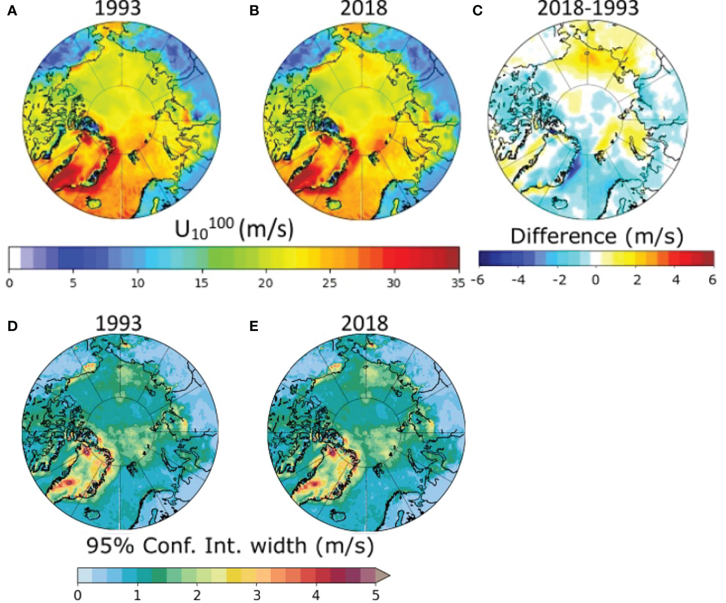
Figure 4 ($U_{10}^{100}$) (ms^-1) obtained with a POT analysis (90^th percentile threshold) and a GPD distribution with the TS-EVA nonseasonal approach for (A) 1993 and (B) 2018. (C) The difference between estimates for 2018 and 1993. Width of 95% confidence interval for $U_{10}^{100}$ for (D) 1993 and (E) 2018.

The TS-EVA analysis, nevertheless, shows that extremes have only been changing marginally for the past three decades (Figure 4). The long term trends of $U_{10}^{100}$ are shown in Figure 5, which reports areal averages as a function of time for each sub-region. In the Atlantic sector, $U_{10}^{100}$ showed a weak drop in the Norwegian and Greenland seas, with a total decrease of about 3ms^-1 over the period 1993-2018 (a rate of -0.12ms^-1 per year). More significant drops were recorded along the Western coast of Greenland (i.e. Fram Strait, Eastern Greenland sea), where $U_{10}^{100}$ reduced at a rate of -0.24ms^-1 per year. The Baffin Bay and the Barents sea showed negligible changes, with $U_{10}^{100}$ remaining approximately constant. The opposite trend was reported on the Eastern side of the Atlantic sector (i.e. the Kara sea), where wind speed showed a weak increase with a rate of 0.04ms^-1 per year. The Pacific sector, on the contrary, was subjected to more consistent trends across the sub-regions. The East Siberian and Chukchi seas show weak positive trends of about 0.16 and 0.12 ms^-1 per year, respectively. A similar increase was also observed in the Western part of the Beaufort sea. The Laptev sea recorded the lowest rate of increase in the Pacific sector, with $U_{10}^{100}$ increasing at a rate of 0.04ms^-1 per year.

FIGURE 5

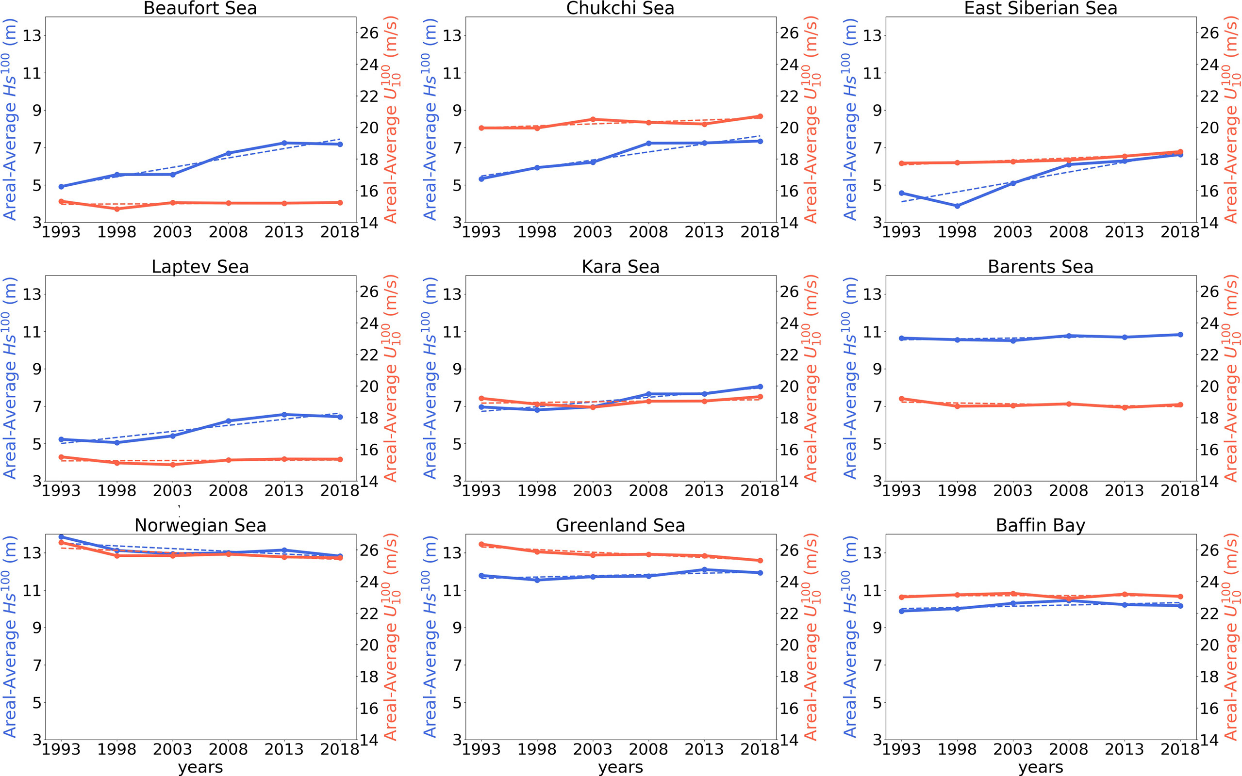
Figure 5 Temporal variation of the Areal-averages of $H_s^{100}$ (blue) and $U_{10}^{100}$ (red) estimated by nonseasonal TS-EVA approach for each sea in the Arctic Ocean.

3.2 Wave Extremes

The energy content of the sea state is historically represented by the significant wave height (Hs, see Holthuijsen 2007), which is used to describe wave extremes. Figure 6 shows the 100-year return levels for significant wave height ($H_s^{100}$), confidence intervals and differences between years 1993 and 2018. It should be noted that regions covered by sea ice for most of the year are not considered in this analysis and thus they are colour-coded with white in the figure. The Atlantic sector experiences high $H_s^{100}$ (>10 m) due to the energetic North Atlantic swell penetrating the Arctic Ocean. Likewise, the Pacific sector experiences significant values of $H_s^{100}$ (>5 m), despite a substantial sea ice cycle that limits fetch lengths for a large fraction of the year. Generally, the 95% confidence intervals vary within ±1.5m at the beginning of the examined period (1993) and widen in more recent years (2018) in regions of significant sea ice decline (see Figures 6D, E), with range increasing up to ±2.5m.

FIGURE 6

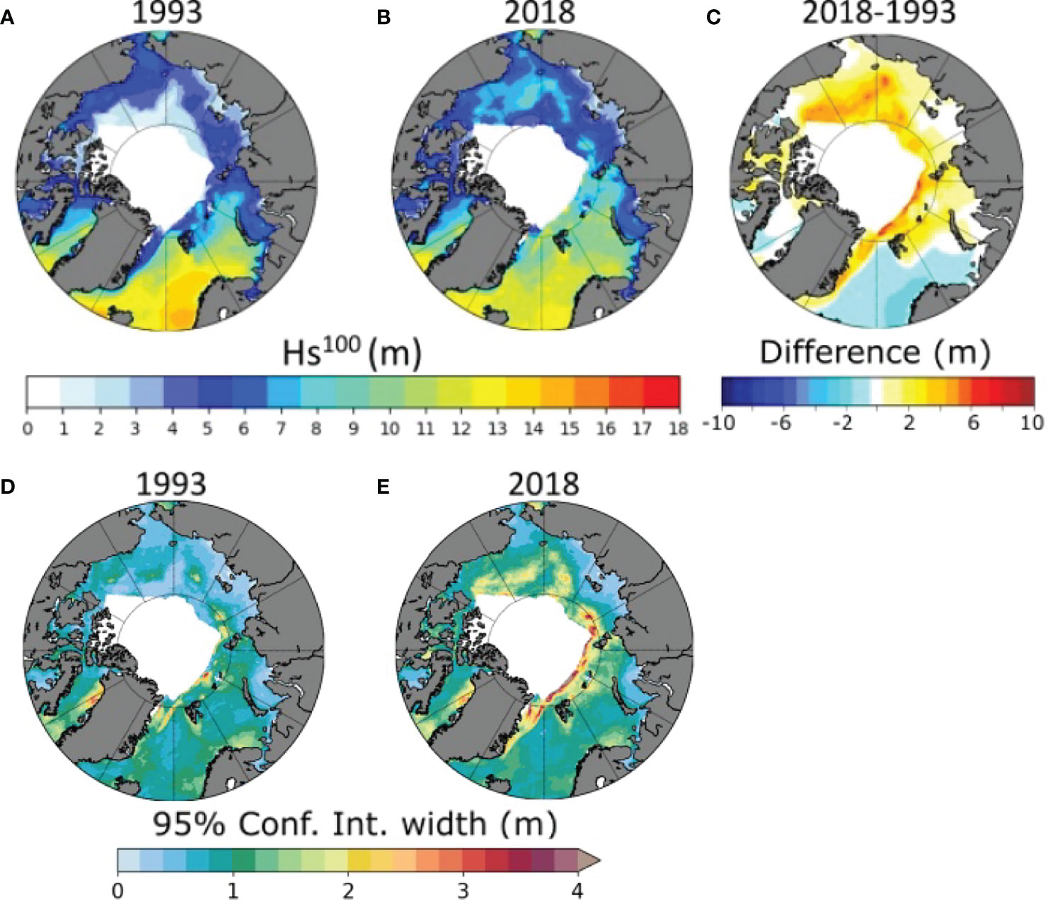
Figure 6 $H_s^{100}$ (m) obtained with a POT analysis (90^th percentile threshold) and a GPD distribution in the TS-EVA nonseasonal approach for (A) 1993 and (B) 2018. (C) The difference between estimations for 2018 and 1993. Width of 95% confidence interval for $H_s^{100}$ for (D) 1993 and (E) 2018.

There is a clear difference of $H_s^{100}$ between 1993 and 2018. More specifically, $H_s^{100}$ increases substantially, up to 4 m, in the emerging open waters of the Pacific sector (the Beaufort, Chukchi and East Siberian seas, cf. sea ice margins in Figure 1). Variations are typically smaller in the Laptev and Kara seas, with increments of about 2 m, on average. Notable increases of $H_s^{100}$ (up to 6 m) occur nearby the sea ice margins. Here, the seasonal sea ice cycle is still significant, introducing uncertainties related to the exact position of sea ice and limiting the amount of data available for the analysis that result in larger confidence intervals (up to ± 4 m). Extremes in the Atlantic sector, surprisingly, show an overall decrease, with $H_s^{100}$ dropping by about 1-2 m. Note, however, that this is a region in which the sea ice extent has not changed dramatically over this period and the decrease is a direct consequence of the drop of wind speed (see Figure 4). Similarly to the Laptev and Kara seas, regions closer to sea ice such as the Fram straits and the Northern part of the Barents sea experienced a sharp growth, with $H_s^{100}$ increasing up to 5 m between 1993 and 2018 (but with notably large uncertainties).

Temporal variations of the aerial average of $H_s^{100}$ are reported in Figure 5 for different basins. A consistent increase of $H_s^{100}$ is evident in the emerging open waters of the Beaufort, Chukchi, East Siberian, Laptev and Kara seas. Variations in the Beaufort and East Siberian seas are the largest, with a total increase over the period 1993-2018 of approximately 16 cm per year. The Chukchi and Laptev seas also experienced a substantial growth of $H_s^{100}$ , with an increase of 6 cm per year, while $H_s^{100}$ increased by approximately 4 cm per year in the Kara sea. In contrast, the Atlantic sector reports only weak upward trends, with the Baffin Bay and Greenland sea showing an increase of 1.6 cm per year. The Barents sea experienced no notable long-term variations, while the Norwegian sea reported a drop in $H_s^{100}$ of about 4 cm per year. We note that, as these latter regions are predominantly free from sea ice, the downward trends are associated with the decline of wind speeds over the North Atlantic (results are consistent with finding in Breivik et al., 2013; Bitner-Gregersen et al., 2018). It is worth noting that negative trends for the North Atlantic are expected to continue in the future as indicated by projections based on RCP 4.5 and RCP 8.5 emission scenarios (Aarnes et al., 2017; Morim et al., 2019). Wave height, however, is predicted to increase at high latitudes of the Norwegian and Barents seas over the next decades as a result of ice decline (Aarnes et al., 2017), confirming the positive trend in wave extremes that is already arising close the ice edge (see Figure 6). The contrast between an overall decrease of wave height as a result of wind speed decline and the increase of wave height due to emerging open waters in winter is also a distinct feature in the North Pacific (cf. Shimura et al., 2016).

The increase in $U_{10}^{100}$ is small over the modelled period (up to about 5% and confined to the Chukchi and Kara Seas; Figure 4C) and it cannot fully explain the more substantial increase of $H_s^{100}$ (up to about 60%; Figure 6C) that is observed around the entire Arctic Ocean, with the Beaufort, Chukchi, East Siberian and Laptev seas being the most significant examples. Nevertheless, it can still be argued that the increase in $H_s^{100}$ is caused by an increase in magnitude/frequency of storms or changes in wind direction. It should be noted, however, that increases in either the magnitude or frequency of storms would also results in notable changes in $U_{10}^{100}$, which are not reported herein. Changes in the prevailing wind directions over Beaufort, Chukchi and East Siberian seas have been reported but are only marginal (Stegall and Zhang, 2012), further suggesting that direct contributions from the wind field are negligible. Conversely, sea ice decline correlates more robustly with the increase of $H_s^{100}$ as substantiated by the temporal variation of the yearly, aerial average of sea ice area in Figure 7 and aerial average of $H_s^{100}$ in Figure 5 (see also the remarkable agreement between regions where $H_s^{100}$ has increased significantly, Figure 6C, and the areas where sea-ice has decreases, Figure 1). Therefore, negative trends of sea ice area remain the most robust cause for longer fetches in emerging open waters, contributing to more effective atmospheric forcing and driving waves to grow in magnitude. This coincides with an enhanced stage of development for the wave fields associated with the 100-year return level, as demonstrated by positive trends of the 100-year wave age (WA¹⁰⁰; Figure 7). The latter is a measure of the strength of the wind forcing and wave growth, and it is computed as $C_p^{100}/U_{10}^{100}$, where $C_p^{100}$ is the phase speed linked to the 100-year peak wave period, which is estimated from a population of peak wave periods associated with the selected significant wave height events (cf. Ochi, 2005). In addition, it is also worth mentioning that regions mostly free of sea-ice, such as the Greenland Sea, have shown very little change in $H_s^{100}$ and WA¹⁰⁰ (Figures 5, 7).

FIGURE 7

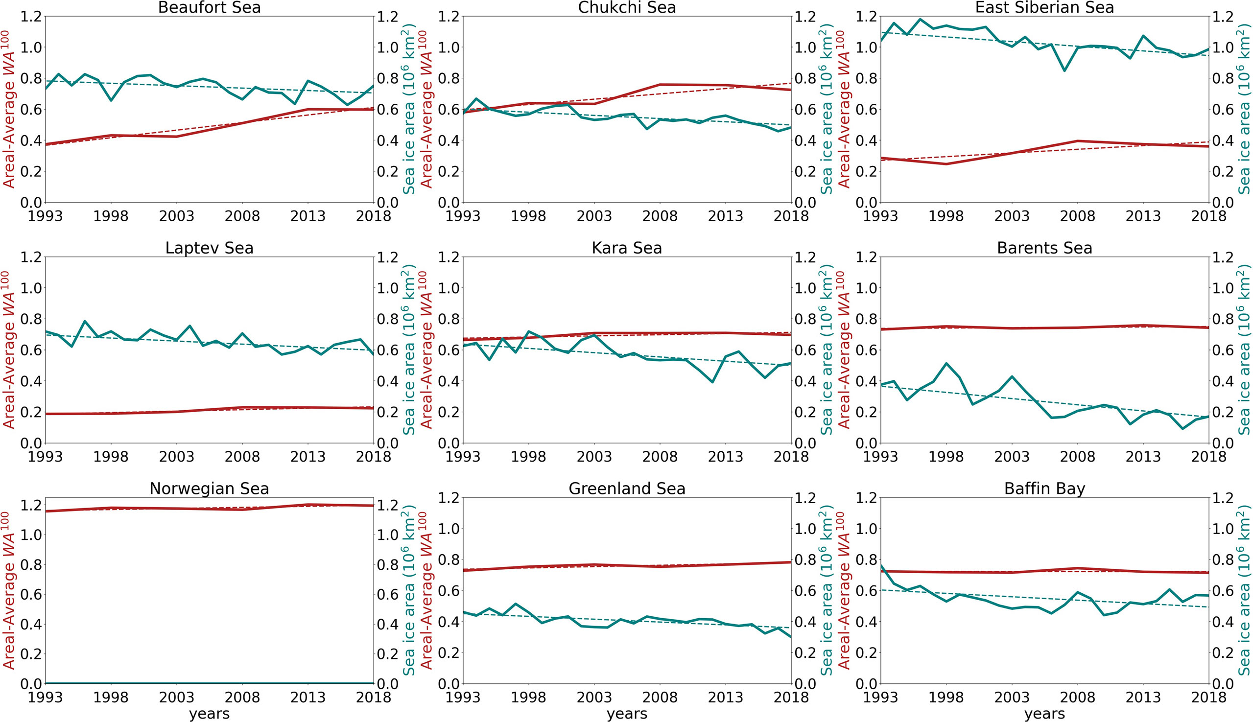
Figure 7 Temporal variation of the yearly areal-average of sea ice area (sea ice extent, blue line) and aerial-average of wave age associated with 100-year events (red line). Areal trends are shown as dashed lines.

4 Seasonal Variability

4.1 Wind Extremes

Figures 8, 9 show the monthly values of $U_{10}^{100}$ for 1993 and 2018, respectively. During the autumn and winter season (October to February), $U_{10}^{100}$ ranges between 20 and 30ms^-1, with peaks along the Greenland coast (Denmark and Fram Straits) up to 50ms^-1. In the spring and summer months (March to September), $U_{10}^{100}$ ranges between 10 and 30ms^-1 with again the highest winds reported in the western Greenland sea. Note that the seasonal approach returns a geographical distribution of extremes that is similar to the one obtained with the nonseasonal approach, but it captures more extreme season-related events. The seasonal component tends to shift the tail of the time-varying extreme value distribution into higher frequencies, resulting in higher estimated extremes for all seasons (months).

FIGURE 8

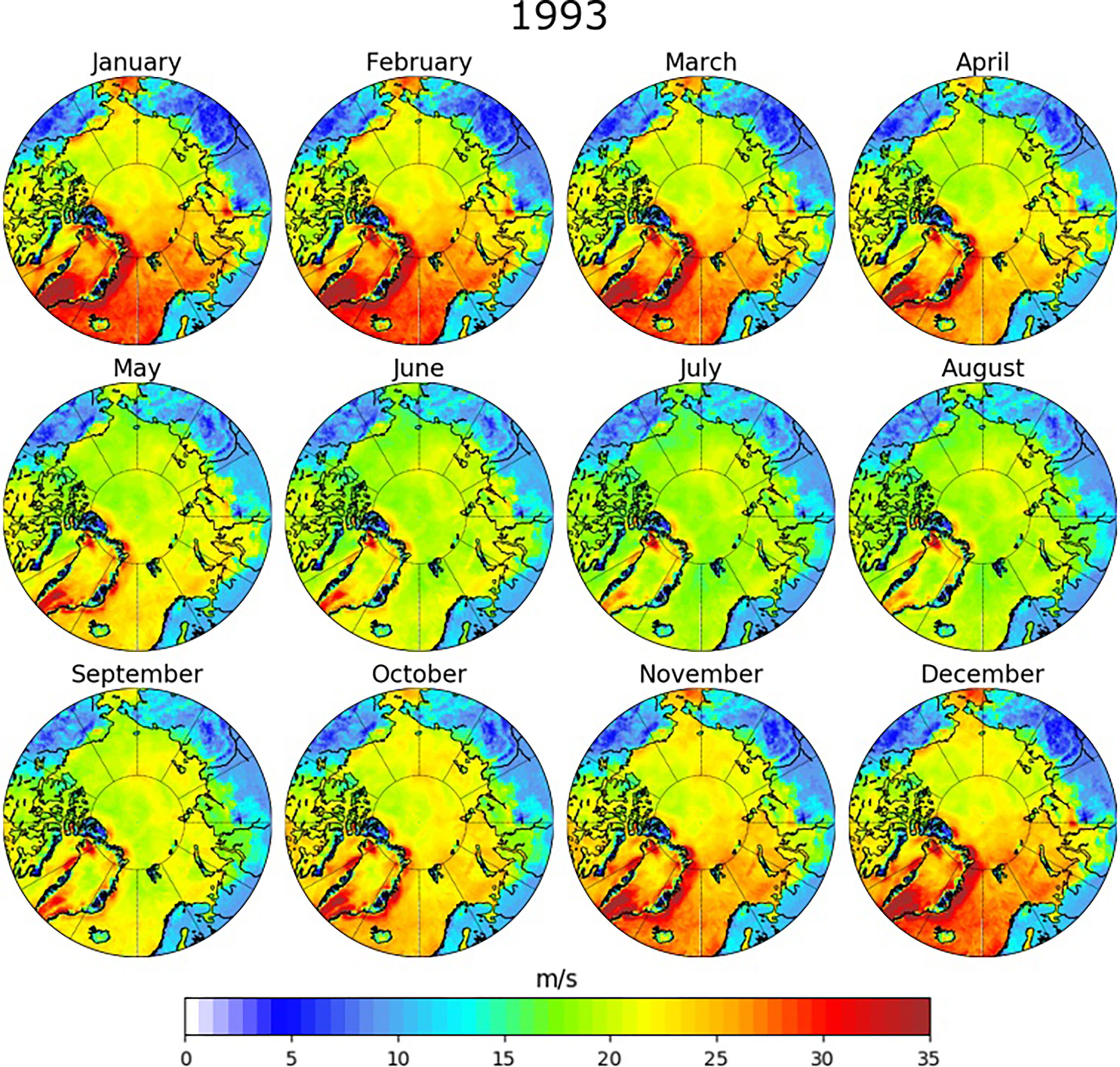
Figure 8 $U_{10}^{100}$ (ms^-1) for 1993 obtained with a POT analysis and a GPD distribution for the TS-EVA seasonal approach. Data obtained from the ERA5 dataset.

FIGURE 9

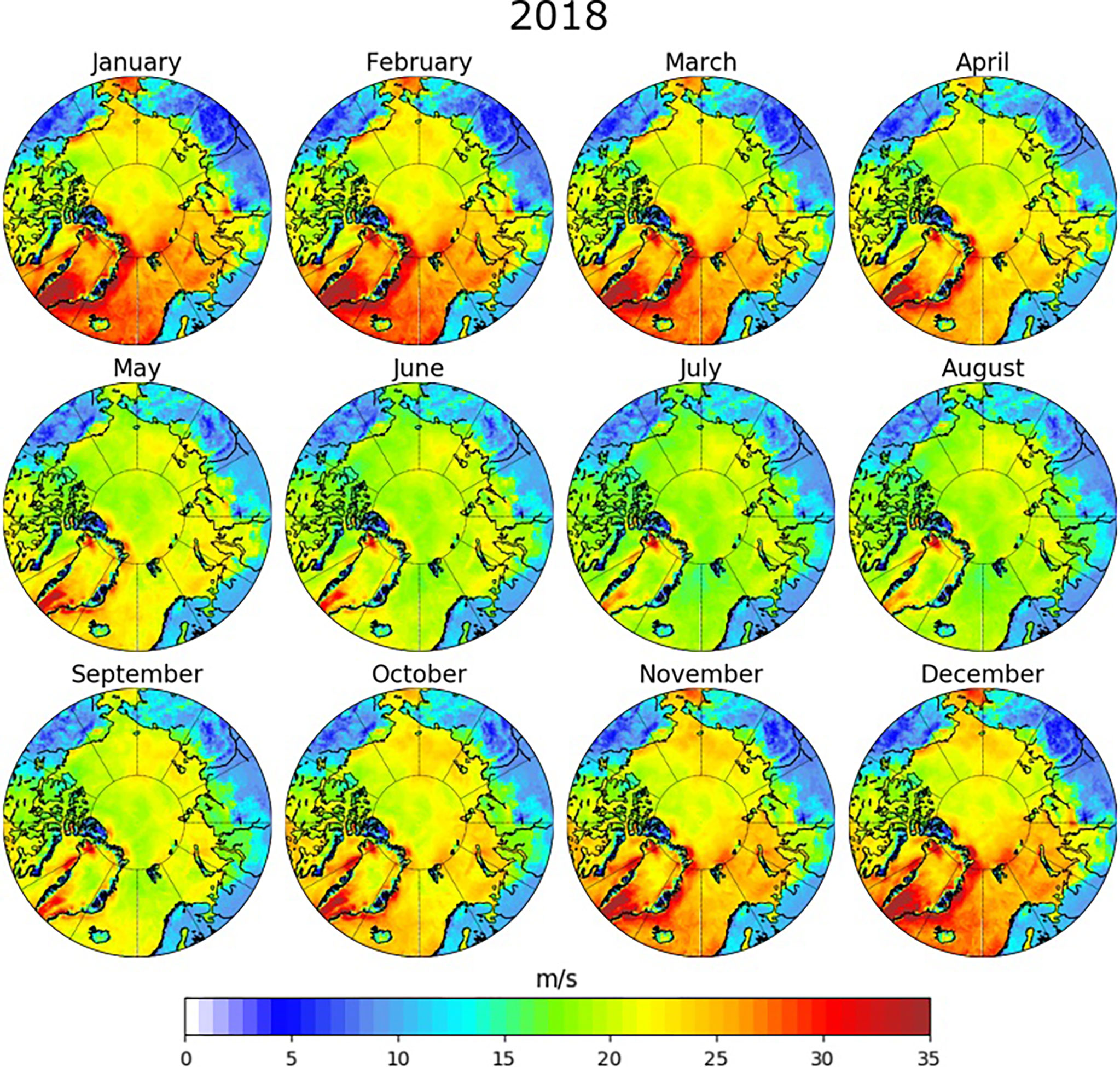
Figure 9 $U_{10}^{100}$(ms^-1) for 2018 obtained with a POT analysis and a GPD distribution for the TS-EVA seasonal approach. Data obtained from the ERA5 dataset.

Differences between $U_{10}^{100}$ for 1993 and 2018 are reported in Figure 10. Generally, differences range between 1 and 3ms^-1 and are quite consistent across all seasons. The Pacific sector experiences an increase, while the Atlantic sector and the central Arctic are subjected to a reduction of $U_{10}^{100}$. The most significant changes are observed in the western Greenland sea during the winter season (December to February), where reductions up to -5ms^-1 were detected. It is interesting to note that the regional distribution of differences is similar for each month, denoting a homogeneous change of extreme winds across the Arctic Ocean throughout the year. Note also that differences obtained with the seasonal approach are consistent with those estimated with the nonseasonal method.

FIGURE 10

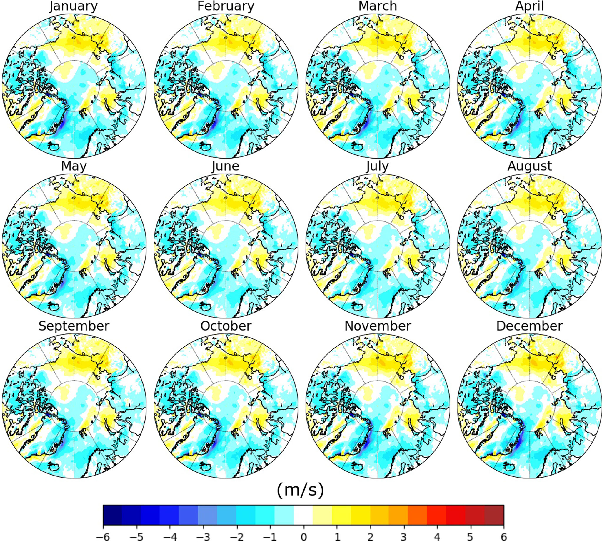
Figure 10 Monthly differences in $U_{10}^{100}$ between estimates for 2018 and 1993.

4.2 Wave Extremes

The seasonal variations of $H_s^{100}$ are presented in Figures 11, 12 for 1993 and 2018, respectively. The minimum sea ice coverage in 1991-1993 is shown as a dashed lines in Figure 12. Extreme wave height, as expected, is subjected to a substantial seasonal variation. The highest values are found in the region encompassing the Greenland and Norwegian Seas, where energetic swells coming from the North Atlantic Ocean propagate into the region (cf. Liu et al., 2016; Stopa et al., 2016). The highest $H_s^{100}$ in this region reaches values up to 18 m in the winter months (December to February), concomitantly with strong winds (Figures 8, 9), and reduces to about 5 m in the summer (June and July). Over the past three decades, however, the general trend shows a consistent reduction in this region at a rate of 4 cm per year regardless of the season (see maps of differences in Figure 13 and trends of areal-averages in Figure 14). These results are in agreement with the results obtained with the nonseasonal approach. Nevertheless, extreme waves penetrate further North in the emerging open waters of the Northern Greenland, Barents and Kara seas, especially during the autumn (September to November) and winter (December to February) seasons in recent years. Consequently, there is a dramatic increase of $H_s^{100}$ in these regions with values up to 13 m in 2018. This corresponds to an average increasing rate of approximately 12 cm per year, with peaks of about 35 cm per year nearby the sea ice margins. Based on future projection, this positive trend is expected to continue (Aarnes et al., 2017).

FIGURE 11

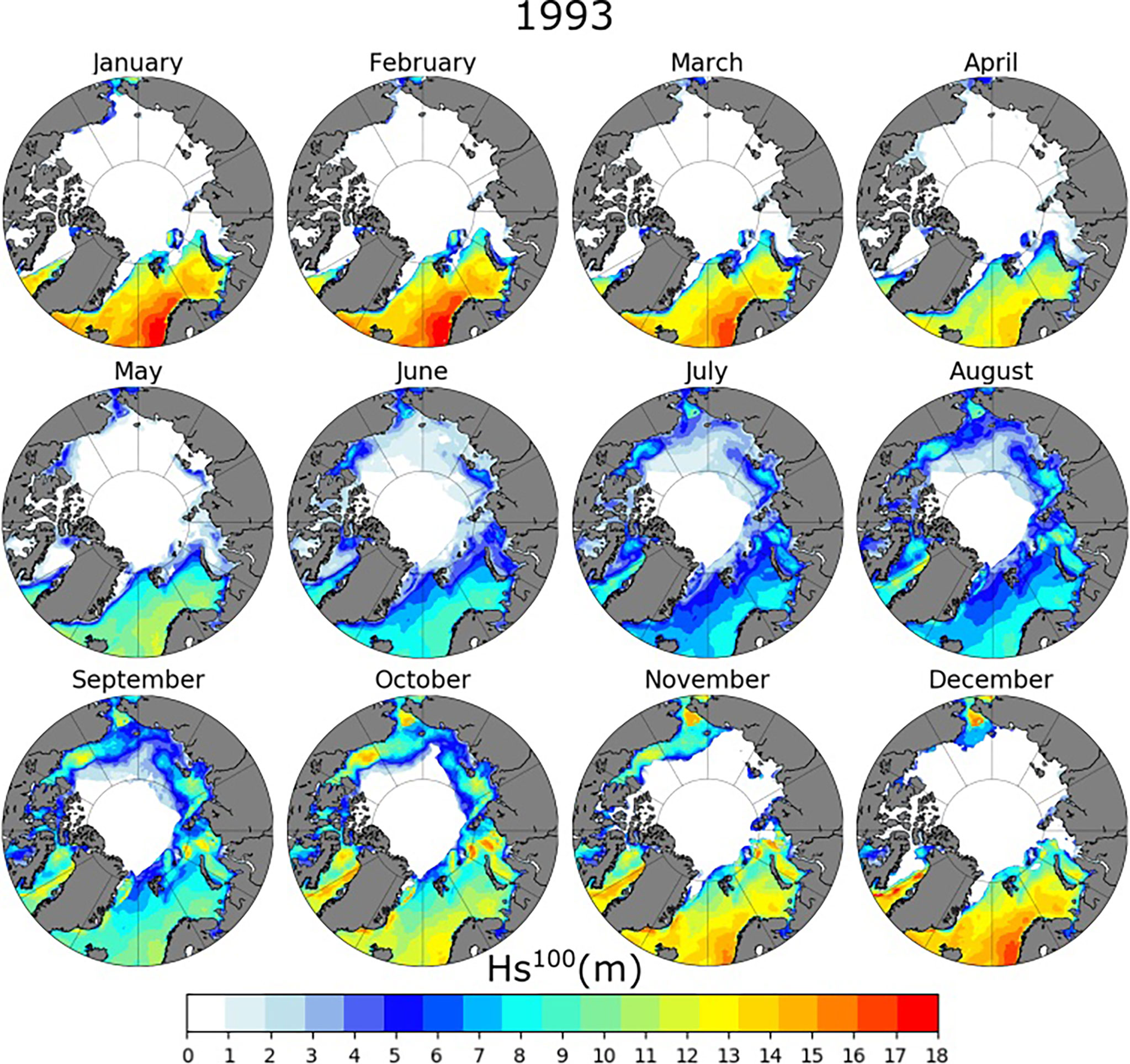
Figure 11 $H_s^{100}$ (m) for 1993 obtained with a POT analysis and a GPD distribution for the TS-EVA seasonal approach. Data obtained from the 28-year wave hindcast with ERA5 wind forcing.

FIGURE 12

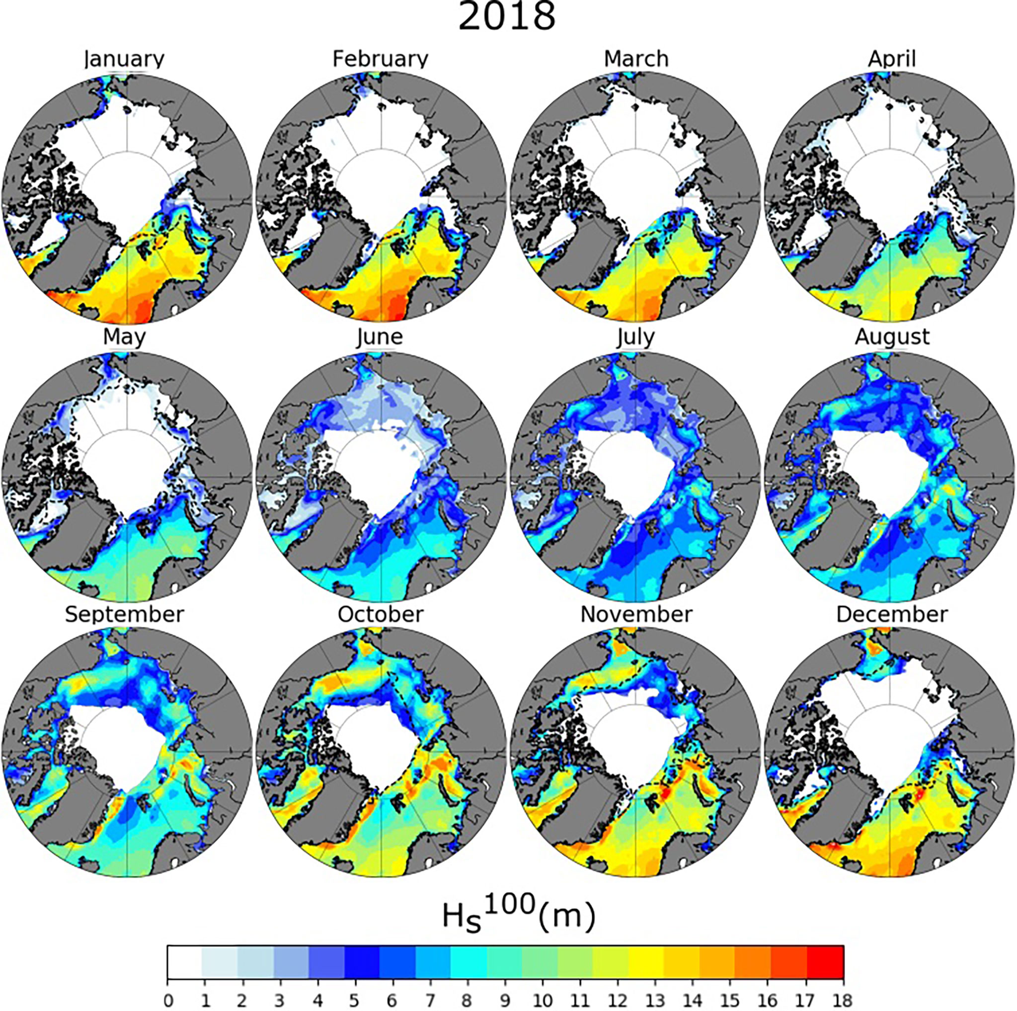
Figure 12 $H_s^{100}$ (m) for 2018 obtained with a POT analysis and a GPD distribution for the TS-EVA seasonal approach. Data obtained from the 28-year wave hindcast with ERA5 wind forcing. Dashed lines represent the minimum sea ice coverage in the period between 1991-1993 for each month.

FIGURE 13

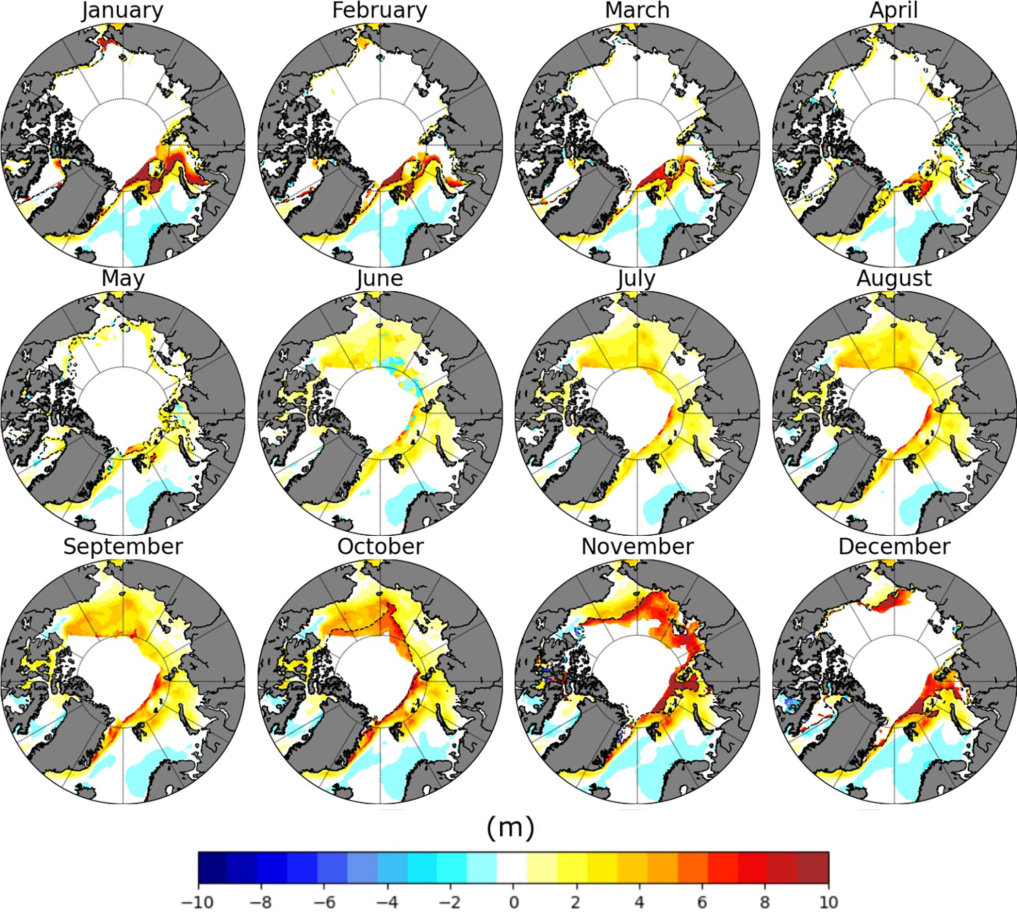
Figure 13 Monthly differences in $H_s^{100}$ between estimates for 2018 and 1993. Dashed lines represent the minimum sea ice coverage in the period between 1991-1993 for each month.

FIGURE 14

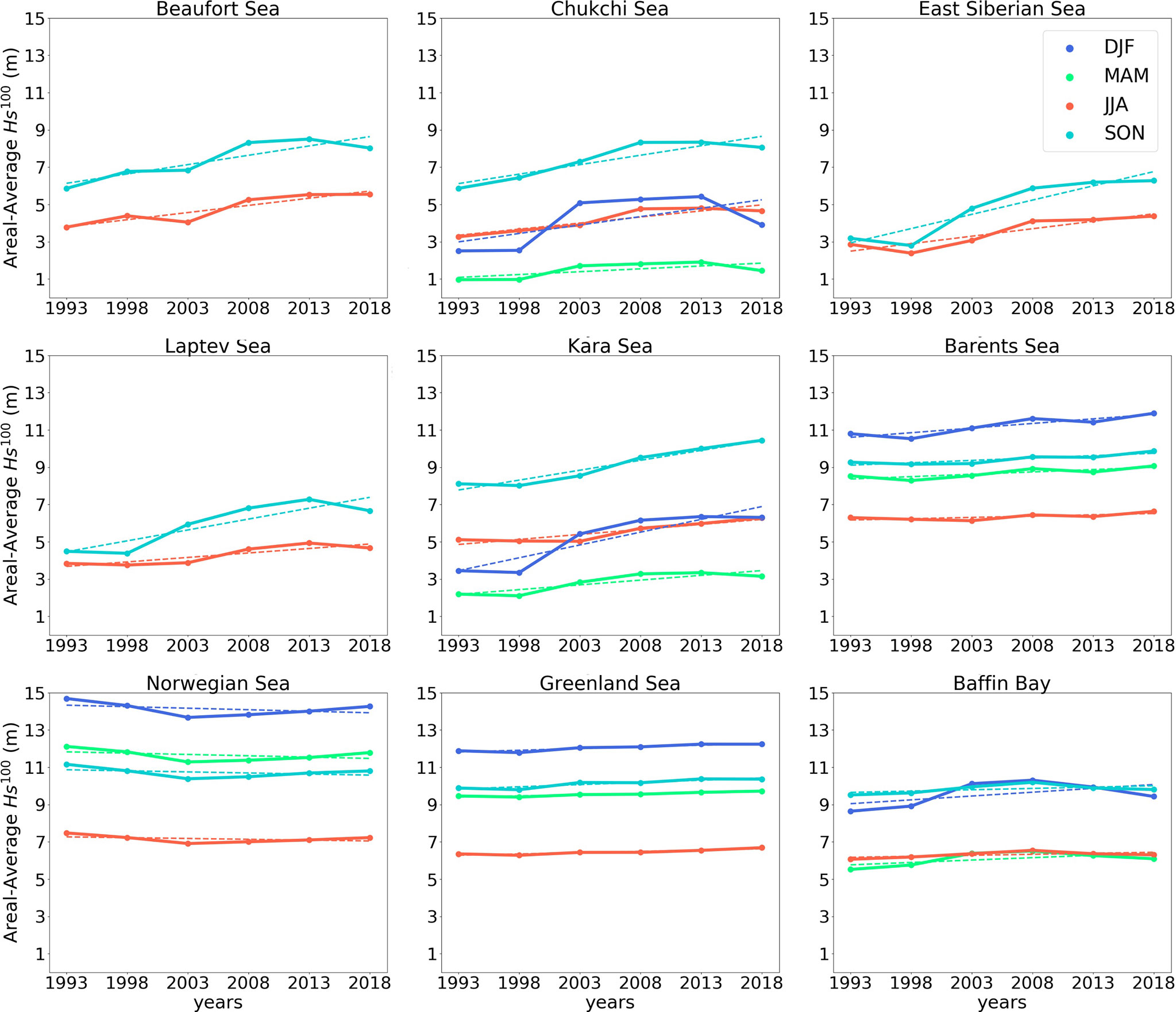
Figure 14 Areal-averages of $H_s^{100}$ in meters estimated by the seasonal TS-EVA approach for each sea in the Arctic Ocean for winter (blue), spring (light green), summer (red), and autumn (light blue).

In regions subjected to the sea ice cycle, wave extremes in 1993 used to build up in late spring or early summer (June), and reach their maximum of up to 12 m in a confined area of the Beaufort sea in autumn (October). In more recent years (2018), extreme waves already have a significant presence earlier in spring (May), primarily in the coastal waters of the Beaufort sea and the East Siberian sea (Figure 13). From June to November, there is a rapid intensification of the sea state and extremes span from a few metres in June to about 16 m in November, with an average growth rate of 12 cm per year, over a region encompassing the whole Beaufort, Chukchi and East Siberian seas. These secluded areas, which are the most prone to positive long-term variations of wind speed (Figure 10) and sea ice retreat (see Figure 7 and Strong and Rigor, 2013), are now experiencing sea state extremes comparable to those reported in the North Atlantic. It is also worth noting that significant changes are also apparent for the western part of the East Siberian sea and the nearby Laptev sea at the end of autumn (November). These regions, which used to be entirely covered by sea ice by November in the earliest decade, are now still completely open with $H_s^{100}$ recording changes up to 8 m (a rate of 32 cm per year since 1993).

5 Discussion

A non-stationary extreme value analysis (TS-EVA, Mentaschi et al., 2016) was applied to assess long-term and seasonal variability of wind and wave extremes (100-year return period levels) in the Arctic Ocean. This non-conventional approach is dictated by the highly dynamic nature of the Arctic, which has been undergoing profound changes over the past decades (Liu et al., 2016; Stopa et al., 2016) and invalidating the basic hypothesis of stationarity that is fundamental for classical extreme value analysis. Estimation of extremes was based on a 28-year (1991-2018) database of 10-metre wind speed and significant wave height, with a temporal resolution of three hours. Wind speed was obtained from the ERA5 reanalysis database and subsequently used to force the WAVEWATCH III spectral wave model. An Arctic Polar Stereographic Projection grid with a horizontal resolution spanning from 9 to 22 km was applied. The model was calibrated and validated against satellite altimeter observations, producing good agreement with a correlation coefficient R = 0.97, scatter index SI = 16% and root mean squared error RMSE =.036m.

The TS-EVA extreme value analysis consisted of transforming the original non-stationary time series of wind speed and wave height into a stationary counterpart and then applying standard peak-over-threshold methods to evaluate extreme values with a return period of 100 years over a running window of 5 years. Non-stationarity was then reinstated by back-transforming the resulting extreme value distribution. Two different approaches were applied to the data sets: a nonseasonal approach, which returns yearly estimates of extremes and enables evaluation of long-term variability; and a seasonal approach, which incorporates a seasonal variability enabling estimation of extremes for specific months.

The nonseasonal approach showed a weak long term variability for the 100-year return period values of wind speed. An increase of approximately 3ms^-1 from 1993 to 2018 (a rate of ≈ 0.12 ms^-1 per year since 1993) was reported in the Pacific sector, especially in the regions of the Chukchi and East Siberian seas and, more marginally, in the Beaufort sea and part of the Laptev sea. A decrease of roughly 31ms^-1 (-0.12ms^-1per year) was found in most of the remaining regions of the Arctic, with peaks in the Eastern part of the Greenland sea (≈ -0.2ms^-1 per year). Conversely, the growth in wave extremes is dramatic and it cannot be attributed to these mild trends in wind extremes, noting that the latter also exclude feedback from possible increases in magnitude/frequency of storms. As wind direction is steady over the Arctic Ocean, changes in the wave field are primarily driven by the substantially longer fetches emerging from sea ice decline that allow waves to build up more energy despite a marginal increase of wind speed. Large changes, in this respect, were found in the Pacific sector encompassing the area between the Beaufort and East Siberian seas, where wave height extremes have been increasing at a rate of approximately 12 cm per year, which results in an overall increase of ≈ 60% from 1993 to 2018. The enhanced wave climate in the Beaufort sea is particularly remarkable since wind extremes are stable and sea ice area is reduced by about 13% during the past three decades (Figures 5, 7), reinforcing the argument that sea ice decline exerts a positive feedback on fetches and, concurrently, wave growth as substantiated by the robust increasing trend of wave age, a measure of the strength of wind forcing and wave growth (Figure 7). The Atlantic sector, on the contrary, experienced a notable decrease of wave extremes at the rate of -4 cm per year; this is consistent with a reduction of wind extremes and with general climate trends observed in Liu et al. (2016). For regions closer to the sea ice edge, where emerging open waters have been replacing pack ice, the 100-year return period levels of wave height exhibit the opposite trend, with a sharp increase of wave extremes at an extremely large local rate of 35 cm per year. It should be noted, however, that estimates of long term trends closer to the sea ice edge are more uncertain due to lack of data in the earlier years, where sea ice covered the ocean more substantially. Nevertheless, it is worth reflecting on the consequences that a sharp upward trend of wave extremes can have on already weak sea ice. As extremes become more extreme, there is negative feedback accelerating sea ice dynamics (Vichi et al., 2019; Alberello et al., 2020; Alberello et al., 2021), break up (Passerotti et al., 2022) and melting processes (Dolatshah et al., 2018), further contributing to sea ice retreat.

The seasonal approach shows a more detailed picture of climate, providing a combined seasonal and long-term variability. Wind extremes distribute uniformly over the Arctic, with peaks in the autumn and winter periods spanning from 20ms^-1 in the Pacific sector to 30ms^-1 in the North Atlantic. Spring and summer months still exhibit significant extremes up to 20ms^-1, with a more homogeneous regional distribution. Over the entire 28-year period, trends are mild and stable through the seasons, consistent with those found with the nonseasonal approach. Variability of wave extremes is again more substantial than wind. In the Pacific sector, the decline of sea ice extent allows a rapid intensification of extremes in the spring (May and June); average growth rates span from 1 cm per year in spring to 12 cm per year in late summer and early autumn. In the Atlantic sector, in response to a notable drop of wind speed, a consistent decrease of wave extremes results all year-round. Nevertheless, the emerging waters of northern Greenland and Barents sea showed the opposite trend with an increase of wave height at a very large rate up to 32 cm per year closer to the sea ice margin.

Data Availability Statement

The datasets presented in this study can be found at https://doi.org/10.5281/zenodo.5592192.

Author Contributions

All authors conceived the manuscript. IC set up the wave model, performed numerical simulations and analysed model output. All authors contributed to the data interpretation and to the writing of the manuscript. All authors contributed to the article and approved the submitted version.

Funding

This research was partially supported by the Victoria Latin America Doctoral Scholarship (VLADS) program.

Conflict of Interest

The authors declare that the research was conducted in the absence of any commercial or financial relationships that could be construed as a potential conflict of interest.

Publisher’s Note

All claims expressed in this article are solely those of the authors and do not necessarily represent those of their affiliated organizations, or those of the publisher, the editors and the reviewers. Any product that may be evaluated in this article, or claim that may be made by its manufacturer, is not guaranteed or endorsed by the publisher.

Acknowledgments

AT acknowledge technical support from the Air-Sea-Ice Lab initiative.

References

Aarnes O. J., Reistad M., Breivik Ø., Bitner-Gregersen E., Ingolf Eide L., Gramstad O., et al. (2017). Projected Changes in Significant Wave Height Toward the End of the 21st Century: Northeast Atlantic. J. Geophys. Res.: Oceans 122, 3394–3403. doi: 10.1002/2016JC012521

CrossRef Full Text | Google Scholar

Alberello A., Bennetts L., Heil P., Eayrs C., Vichi M., MacHutchon K., et al. (2020). Drift of Pancake Ice Floes in the Winter Antarctic Marginal Ice Zone During Polar Cyclones. J. Geophys. Res.: Oceans 125, e2019JC015418. doi: 10.1029/2019JC015418

CrossRef Full Text | Google Scholar

Alberello A., Dolatshah A., Bennetts L. G., Onorato M., Nelli F., Toffoli A. (2021). A Physical Model of Wave Attenuation in Pancake Ice. Int. J. Offshore Polar Eng. 31, 263–269. doi: 10.17736/ijope.2021.ik08

CrossRef Full Text | Google Scholar

Alves J. H. G., Young I. R. (2003). On Estimating Extreme Wave Heights Using Combined Geosat, Topex/Poseidon and ERS-1 Altimeter Data. Appl. Ocean Res. 25, 167–186. doi: 10.1016/j.apor.2004.01.002

CrossRef Full Text | Google Scholar

Amante C., Eakins B. W. (2009). ETOPO1 Arc-Minute Global Relief Model: Procedures, Data Sources and Analysis. (Boulder, Colo: U.S. Dept. of Commerce, National Oceanic and Atmospheric Administration, National Environmental Satellite, Data, and Information Service, National Geophysical Data Center, Marine Geology and Geophysics Division).

Google Scholar

Bitner-Gregersen E. M., Bhattacharya S. K., Chatjigeorgiou I. K., Eames I., Ellermann K., Ewans K., et al. (2014). Recent Developments of Ocean Environmental Description With Focus on Uncertainties. Ocean Eng. 86, 26–46. doi: 10.1016/j.oceaneng.2014.03.002

CrossRef Full Text | Google Scholar

Bitner-Gregersen E. M., Toffoli A. (2014). Occurrence of Rogue Sea States and Consequences for Marine Structures. Ocean Dynamics 64, 1457–1468. doi: 10.1007/s10236-014-0753-2

CrossRef Full Text | Google Scholar

Bitner-Gregersen E. M., Vanem E., Gramstad O., Hørte T., Aarnes O. J., Reistad M., et al. (2018). Climate Change and Safe Design of Ship Structures. Ocean Eng. 149, 226–237. doi: 10.1016/j.oceaneng.2017.12.023

CrossRef Full Text | Google Scholar

Breivik Ø., Aarnes O. J., Abdalla S., Bidlot J.-R., Janssen P. A. (2014). Wind and Wave Extremes Over the World Oceans From Very Large Ensembles. Geophys. Res. Lett. 41, 5122–5131. doi: 10.1002/2014GL060997

CrossRef Full Text | Google Scholar

Breivik Ø., Aarnes O. J., Bidlot J. R., Carrasco A., Saetra Ø. (2013). Wave Extremes in the Northeast Atlantic From Ensemble Forecasts. J. Climate 26, 7525–7540. doi: 10.1175/JCLI-D-12-00738.1

CrossRef Full Text | Google Scholar

Cabral I., Young I. R., Toffoli A. (2021). Arctic Wave Hindcast. doi: 10.5281/zenodo.5592193

CrossRef Full Text | Google Scholar

Caires S., Steri A. (2021). 100-year return value estimates for ocean wind speed and significant wave height from the era-40 data. J. Climate 18, 1032–1048.

Google Scholar

Casas-Prat M., Wang X. L. (2020). Sea-Ice Retreat Contributes to Projected Increases in Extreme Arctic Ocean Surface Waves. Geophys. Res. Lett. 47, e2020GL088100. doi: 10.1029/2020GL088100

CrossRef Full Text | Google Scholar

Cheng L., AghaKouchak A., Gilleland E., Katz R. W. (2014). Non-Stationary Extreme Value Analysis in a Changing Climate. Climatic Change 127, 353–369. doi: 10.1007/s10584-014-1254-5

CrossRef Full Text | Google Scholar

Chu J., Dickin O., Nadarajah S. (2019). A Review of Goodness of Fit Tests for Pareto Distributions. J. Comput. Appl. Math. 361, 13–41. doi: 10.1016/j.cam.2019.04.018

CrossRef Full Text | Google Scholar

Clancy C., O’Sullivan J., Sweeney C., Dias F., Parnell A. C. (2016). Spatial Bayesian Hierarchical Modelling of Extreme Sea States. Ocean Modelling 107, 1–13. doi: 10.1016/j.ocemod.2016.09.015

CrossRef Full Text | Google Scholar

Coles S., Bawa J., Trenner L., Dorazio P. (2001). An Introduction to Statistical Modeling of Extreme Values 208, 208. (London: Springer).

Google Scholar

Dee D. P., Uppala S. M., Simmons A. J., Berrisford P., Poli P., Kobayashi S., et al. (2011). The ERA-Interim Reanalysis: Configuration and Performance of the Data Assimilation System. Q. J. R. meteorol Soc. 137, 553–597. doi: 10.1002/qj.828

CrossRef Full Text | Google Scholar

De Leo F., Besio G., Briganti R., Vanem E. (2021). Non-Stationary Extreme Value Analysis of Sea States Based on Linear Trends. Analysis of Annual Maxima Series of Significant Wave Height and Peak Period in the Mediterranean Sea. Coastal Eng. 167, 103896. doi: 10.1016/j.coastaleng.2021.103896

CrossRef Full Text | Google Scholar

Dolatshah A., Monbaliu J., Toffoli A.. (2022). Interactions Between Irregular Wave Fields And Sea Ice: A Physical Model For Wave Attenuation And Ice Breakup In An Ice Tank, J Phys Oceanogr (published online ahead of print 2022)., doi: 10.1175/JPO-D-21-0238.1

CrossRef Full Text | Google Scholar

Dolatshah A., Nelli F., Bennetts L. G., Alberello A., Meylan M. H., Monty J. P., et al. (2018). Hydroelastic Interactions Between Water Waves and Floating Freshwater Ice. Phys. Fluids 30, 091702. doi: 10.1063/1.5050262

CrossRef Full Text | Google Scholar

Emery W. J., Thomson R. E. (2014). Data Analysis Methods in Physical Oceanography (Amsterdam: Elsevier).

Google Scholar

Fernández L., Calvino C., Dias F. (2021). Sensitivity Analysis of Wind Input Parametrizations in the Wavewatch Iii Spectral Wave Model Using the St6 Source Term Package for Ireland. Appl. Ocean Res. 115, 102826. doi: 10.1016/j.apor.2021.102826

CrossRef Full Text | Google Scholar

Galiatsatou P., Prinos P. (2011). Modeling Non-Stationary Extreme Waves Using a Point Process Approach and Wavelets. Stoch. Env. Res. Risk A 25, 165–183. doi: 10.1007/s00477-010-0448-2

CrossRef Full Text | Google Scholar

Gallagher S., Gleeson E., Tiron R., McGrath R., Dias F. (2016). Twenty-First Century Wave Climate Projections for Ireland and Surface Winds in the North Atlantic Ocean. Adv. Sci. Res. 13, 75–80. doi: 10.5194/asr-13-75-2016

CrossRef Full Text | Google Scholar

Günther F., Overduin P. P., Yakshina I. A., Opel T., Baranskaya A. V., Grigoriev M. N. (2015). Observing Muostakh Disappear: Permafrost Thaw Subsidence and Erosion of a Ground-Ice-Rich Island in Response to Arctic Summer Warming and Sea Ice Reduction. Cryosphere 9, 151–178. doi: 10.5194/tc-9-151-2015

CrossRef Full Text | Google Scholar

Hersbach H., Bell B., Berrisford P., Horányi A., Sabater J. M., Nicolas J., et al. (2019). Global Reanalysis: Goodbye ERA-Interim, Hello ERA5. ECMWF Newsl 159, 17–24. doi: 10.21957/vf291hehd7

CrossRef Full Text | Google Scholar

Holthuijsen L. H.. (2007). Waves in Oceanic and Coastal Waters (Cambridge: Cambridge University Press). doi: 10.1017/CBO9780511618536

CrossRef Full Text | Google Scholar

IPCC. (2019). IPCC Special Report on the Ocean and Cryosphere in a Changing Climate. Pörtner H. O., Roberts D. C., Masson-Delmotte V., Zhai P., Tignor M., Poloczanska E., et al. (eds.) In Press. (Cambridge: Cambridge University Press). doi: 10.1017/CBO9780511618536

CrossRef Full Text | Google Scholar

Jones B. M., Arp C. D., Jorgenson M. T., Hinkel K. M., Schmutz J. A., Flint P. L. (2009). Increase in the Rate and Uniformity of Coastline Erosion in Arctic Alaska. Geophys. Res. Lett. 36, L03503. doi: 10.1029/2008GL036205

CrossRef Full Text | Google Scholar

Kohout A. L., Smith M., Roach L. A., Williams G., Montiel F., Williams M. J. M. (2020). Observations of Exponential Wave Attenuation in Antarctic Sea Ice During the Pipers Campaign. Ann. Glaciol. 61, 196–209. doi: 10.1017/aog.2020.36

CrossRef Full Text | Google Scholar

Komen G. J., Hasselmann K., Hasselmann K. (1984). On the Existence of a Fully Developed Wind-Sea Spectrum. J. Phys. oceanogr. 14, 1271–1285. doi: 10.1175/1520-0485(1984)014<1271:OTEOAF>2.0.CO;2

CrossRef Full Text | Google Scholar

Law-Chune S., Aouf L., Dalphinet A., Levier B., Drillet Y., Drevillon M. (2021). Waverys: A Cmems Global Wave Reanalysis During the Altimetry Period. Ocean Dynamics 71, 357–378. doi: 10.1007/s10236-020-01433-w

CrossRef Full Text | Google Scholar

Liu Q., Babanin A. V., Zieger S., Young I. R., Guan C. (2016). Wind and Wave Climate in the Arctic Ocean as Observed by Altimeters. J. Climate 29, 7957–7975. doi: 10.1175/JCLI-D-16-0219.1

CrossRef Full Text | Google Scholar

Liu Q., Rogers W. E., Babanin A. V., Young I. R., Romero L., Zieger S., et al. (2019). Observation-Based Source Terms in the Third-Generation Wave Model WAVEWATCH III: Updates and Verification. J. Phys. Oceanogr. 49, 489–517. doi: 10.1175/JPO-D-18-0137.1

CrossRef Full Text | Google Scholar

Méndez F. J., Menéndez M., Luceño A., Losada I. J. (2006). Estimation of the Long-Term Variability of Extreme Significant Wave Height Using a Time-Dependent Peak Over Threshold (Pot) Model. J. Geophys. Res.: Oceans 111, C07024. doi: 10.1029/2005JC003344

CrossRef Full Text | Google Scholar

Mentaschi L., Vousdoukas M., Voukouvalas E., Sartini L., Feyen L., Besio G., et al. (2016). The Transformed-Stationary Approach: A Generic and Simplified Methodology for Non-Stationary Extreme Value Analysis. Hydrol. Earth System Sci. 20, 3527–3547. doi: 10.5194/hess-20-3527-2016

CrossRef Full Text | Google Scholar

Meucci A., Young I. R., Breivik Ø. (2018). Wind and Wave Extremes From Atmosphere and Wave Model Ensembles. J. Climate 31, 8819–8842. doi: 10.1175/JCLI-D-18-0217.1

CrossRef Full Text | Google Scholar

Meucci A., Young I. R., Hemer M., Kirezci E., Ranasinghe R. (2020). Projected 21st Century Changes in Extreme Wind-Wave Events. Sci. Adv. 6, eaaz7295. doi: 10.1126/sciadv.aaz7295

PubMed Abstract | CrossRef Full Text | Google Scholar

Morim J., Hemer M., Wang X. L., Cartwright N., Trenham C., Semedo A., et al. (2019). Robustness and Uncertainties in Global Multivariate Wind-Wave Climate Projections. Nat. Climate Change 9, 711–718. doi: 10.1038/s41558-019-0542-5

CrossRef Full Text | Google Scholar

Ochi M. K. (2005). Ocean Waves: The Stochastic Approach (Cambridge: Cambridge Ocean Technology Series). doi: 10.1017/CBO9780511529559

CrossRef Full Text | Google Scholar

Queffeulou P., Croizé-Fillon D. (2015). Global Altimeter SWH Data Set, Version 11.1. Tech. Rep.

Google Scholar

Renard B., Sun X., Lang M. (2013). “Bayesian Methods for Non-Stationary Extreme Value Analysis,” in Extremes in a Changing Climate (Dordrecht: Springer), 39–95.

Google Scholar

Shimura T., Mori N., Hemer M. A. (2016). Variability and Future Decreases in Winter Wave Heights in the Western North Pacific. Geophys. Res. Lett. 43, 2716–2722. doi: 10.1002/2016GL067924

CrossRef Full Text | Google Scholar

Stegall S.T, Zhang J (2012). Wind Field Climatology, Changes, And Extremes In The Chukchi–beaufort Seas And Alaska North Slope During 1979–2009. J. Climate 25, 8075–8089.

Google Scholar

Stopa J. E., Ardhuin F., Girard-Ardhuin F. (2016). Wave Climate in the Arctic 1992–2014: Seasonality and Trends. Cryosphere 10, 1605–1629. doi: 10.5194/tc-10-1605-2016

CrossRef Full Text | Google Scholar

Strong C., Rigor I. G. (2013). Arctic Marginal Ice Zone Trending Wider in Summer and Narrower in Winter. Geophys. Res. Lett. 40, 4864–4868. doi: 10.1002/grl.50928

CrossRef Full Text | Google Scholar

Takbash A, Young I. R. (2019). Global Ocean Extreme Wave Heights From Spatial Ensemble Data. J. Climate 32, 6823–6836.

Google Scholar

Takbash A, Young I.R., Breivik Ø (2019). Global Wind Speed And Wave Height Extremes Derived From Long-duration Satellite Records. J. Climate 32, 109–126.

Google Scholar

Thomson R. E., Emery W. J. (2014). Data Analysis Methods in Physical Oceanography (Newnes). Amsterdam, Elsevier.

Google Scholar

Thomson J., Fan Y., Stammerjohn S., Stopa J., Rogers W. E., Girard-Ardhuin F., et al. (2016). Emerging Trends in the Sea State of the Beaufort and Chukchi Seas. Ocean modelling 105, 1–12. doi: 10.1016/j.ocemod.2016.02.009

CrossRef Full Text | Google Scholar

Thomson J., Rogers W. E. (2014). Swell and Sea in the Emerging Arctic Ocean. Geophys. Res. Lett. 41, 3136–3140. doi: 10.1002/2014GL059983

CrossRef Full Text | Google Scholar

Tolman H. L. (2009). User Manual and System Documentation of WAVEWATCH III TM Version 3.14. Tech. note MMAB Contribution 276, 220.

Google Scholar

Vichi M., Eayrs C., Alberello A., Bekker A., Bennetts L., Holland D., et al. (2019). Effects of an Explosive Polar Cyclone Crossing the Antarctic Marginal Ice Zone. Geophys. Res. Lett. 46, 5948–5958. doi: 10.1029/2019GL082457

CrossRef Full Text | Google Scholar

Vinoth J., Young I.R (2011). Global Estimates of Extreme Wind Speed and Wave Height. J. Climate 24, 1647–1665.

Google Scholar

Waseda T., Webb A., Sato K., Inoue J., Kohout A., Penrose B., et al. (2018). Correlated Increase of High Ocean Waves and Winds in the Ice-Free Waters of the Arctic Ocean. Sci. Rep. 8, 4489. doi: 10.1038/s41598-018-22500-9

PubMed Abstract | CrossRef Full Text | Google Scholar

Zieger S., Babanin A. V., Rogers W. E., Young I. R. (2015). Observation-Based Source Terms in the Third-Generation Wave Model WAVEWATCH. Ocean modelling 96, 2–25. doi: 10.1016/j.ocemod.2015.07.014

CrossRef Full Text | Google Scholar